The FDI-growth nexus in South Africa: A re-examination

Munich Personal RePEc Archive

The FDI-growth nexus in South Africa:

A re-examination using quantile

regression approach

Khobai, Hlalefang and Hamman, Nicolene and Mkhombo,

Thando and Mhaka, Simba and Mavikela, Nomahlubi and

Phiri, Andrew

12 July 2017

Online at https://mpra.ub.uni-muenchen.de/80152/

MPRA Paper No. 80152, posted 13 Jul 2017 13:35 UTC

THE FDI-GROWTH NEXUS IN SOUTH AFRICA: A RE-EXAMINATION USING

QUANTILE REGRESSION APPROACH

H. Khobai

Department of Economics, Faculty of Business and Economic Studies, Nelson Mandela

Metropolitan University, Port Elizabeth, South Africa, 6031.

N. Hamman



T. Mkhombo



S. Mhaka



N. Matolweni



And

A. Phiri



ABSTRACT: This study sought to contribute to the growing empirical literature by

investigating the effects of FDI on per capita GDP growth for South Africa using time series

data collected between 1970 and 2016. In differing from a majority of previous studies we use

quantile regressions which investigates the effects of FDI on economic growth at different

distributional quantiles. Puzzling enough, our empirical results show that FDI has a negative

influence on welfare at extremely low quantiles whereas at other levels this effect turns

insignificant. Contrary, the effects of domestic investment on welfare is positive and significant

at all levels. Collectively, these result have important implications for policymakers in South

Africa.

Keywords: FDI; Economic growth; Quantile regression; Global financial crisis; South Africa.

JEL Classification Code: C21; C31; E22; F43; O40.

1 INTRODUCTION

Since the financial liberalization era of the 1980’s and 1990’s when economies

worldwide began to be increasingly integrated into the global economy, the relationship

between foreign direct investment (FDI) and output growth became subjected to intense

research. FDI is perceived as a major factor in enhancing economic growth, especially in

developing countries where the savings rates are relatively low. In particular, FDI contributes

to the integration of developing countries into the world economy as it provides not only capital

but also technology and management know-how necessary for restructuring firms in the host

countries (Keho, 2015). Nevertheless, the empirical evidence regarding the empirical links

amongst FDI and economic growth remains mixed due to different methodologies employed,

different data usage and different country specifics.

South Africa, as a prominent emerging economy, is often considered to be the gateway

to the Sub-Saharan Africa (SSA) region, as well as being one of the prominent FDI recipients

in terms of national resources, traditional oil as well as minerals. However, prior to the first

democratic elections in 1994, when international sanctions were imposed on the state between

the 1980’s and the early 1990’s, South Africa’s FDI had been close to zero as the country

become increasing isolated from the global economy during that period. Nevertheless,

following the termination of the apartheid regime in the early 1990’s, the new democratic South

Africa government changed the focus of it’s economic development and growth strategy

towards deeper global integration, developing stabilizing macroeconomic policies as well as

attracting increasingly higher numbers of foreign investors.

Over the past two decades, South Africa has become an important global economic

player. In 2012, the country was considered one of the largest recipients of FDI in Africa with

over US$3 billion. According to the United Nations Conference on Trade and Development

(UNCTAB, 2013), South Africa has been receiving a bulk majority of it’s FDI (i.e.

approximately 89%) from the European Union, while other major contributing countries

include the UK with 75.8% and other minor contributors include Germany with 6% and other

developing countries an overall of 4% of FDI to South Africa, of which 2.5% is generated by

Asian economies alone.

Following the global financial crisis of 2007-2008, many economies worldwide are still

recovering from the aftereffects of the global recessionary period of 2009-2010 and the Euro

debt crisis of 2010 which ensued afterwards. Many economies across the globe witnessed

major declines in output, employment and trade. GDP growth worldwide declined drastically

in 2009, dropping from slightly over 4 percent to 0.9 percent between 2007 and 2009.

Moreover, approximately 34 million jobs worldwide were lost during the 2009 recession while

world trade volumes plummeted by more than 40 percent in 2008, collapsing at rate that

outpaced the fall of aggregate output (Alfaro and Chen, 2011). According to the World

Economic Forum, in order for the world to recover from its decline in growth, the global

economy needs an injection of new FDI to reach US$ 3 trillion annually (approximately 4% of

current world gross domestic product, GDP). Hence there has been a recent rejuvenation of

empirical interest concerning the effects of FDI on economic growth.

Nevertheless, we notice two major short-comings associated with a majority of

previous empirical studies addressing the subject matter. Firstly, most studies do not take into

consideration the possible effect of the financial crisis on the FDI-growth relationship.

Secondly, studies suffer from the methodological shortcoming of relying on OLS and other

linear estimating techniques hence assuming that the effects of FDI on economic growth are

uniform across all levels of FDI. In reality, this assumption does not hold true. Therefore, in

our current study we differ from a host majority of previous studies by investigating the effect

of FDI on economic in South Africa over the period of 1970 to 2016 using quantile regression

methodology of Koenker and Bassett (1978). The primary advantage of quantile regression

over least-squares regression is its flexibility for modelling data with heterogeneous

conditional distributions. Therefore, in comparison to other linear estimation techniques

commonly used in the literature, quantile regression provides a more complete covariate picture

of the covariate effect when a set of percentiles is modelled, and makes no distributional

assumption about the error term in the model (Koenker and Hallock (2001).

We henceforth, structure of the remainder of the paper as follows. The next section of

the paper will review the literature concerned with the effects of FDI on economic growth. The

third section will present the econometric model and this will be followed by the data and

empirical analysis which are presented in section four. Section five will conclude the study and

provide recommendations based on the research findings.

2 THEORETICAL REVIEW

2.1 Theories of FDI

Theories of FDI began to more prominently emerge in the post- World War II era. Even

though theories of FDI are wide spread, for convenience sake, we restrict the reviewed

mainstream theories of FDI to those classified under imperfect markets which can further be

categorized into four main theories. Firstly, there is the industrial organization approach of

Hymer (1968 and 1970) and extended upon by Kindelberger (1969) which is consider one of

the earliest explanations of investment flows in an oligopolistic market situations. According

to this theory, when a multinational corporations (MNC’s) establish a subsidiary in a foreign

country it faces several disadvantages in competing with local firms such as culture, language,

legal system and consumers preferences. As initially argued in Kindelberger (1969), these

disadvantages can be offset by some form of market power such as the possession of

proprietary resources and unique capabilities such as differentiated products, proprietary

technology, managerial skills, better access to capital and government imposed market

distortions confer MNCs with competitive advantage over indigenous firms in the host country

and help them offset the disadvantages of operating in a foreign country (Nayyar,2014).

Under the second approach, the transaction cost approach or internalization theory, as

popularized in the works of Buckley and Casson (1976) and Williamson (1979) and yet having

its roots embedded in the seminal works of Coase (1937), FDI is viewed as an organizational

response to market imperfections faced by MNC’s. In particular, the internalization theory

hinges on three postulates i) firms maximize profits in a market that is perfect ii) When markets

in intermediate products are imperfect, there is an incentive to bypass them by creating internal

markets iii) internalization of markets across the worlds leads to MNC’s (Nayak and

Choudhury, 2014). Since intangible assets, such as technology, marketing ability and consumer

goodwill, based largely on proprietary information, they cannot be exchanged at across borders

for a variety of reasons rising from the economics of information as well as from the economics

of public goods (Morck and Young, 1992). The firm thus overcomes these market

imperfections by creating an internal market and this internalization of markets is an on-going

process which continues until the marginal benefits and marginal costs are equal.

The last theory of FDI we discuss the eclectic paradigm of international production as

pioneered by Dunning (1973). In essence, the theory integrates both the internalization and

oligopolistic theories and adds a third dimension in the form of location theory to explain why

firm opens a foreign subsidiary (Nayak and Choudhury, 2014). The theory asserts that, at any

given moment of time, the extent and pattern of international production will be determined by

the configuration of three sets of forces; namely, i) the net competitive ownership MNc’s

possess vis-à-vis foreign firms ii) the extent to which firms perceive it to be in their best

interests to internalize the markets for the generation and/or the use of these assets; and by so

doing add value to them; and iii) the extent to which firms choose to locate these value-adding

activities outside their national boundaries (Nayyar,2014). Combining these three factors,

namely, ownership (O), internalization (I) and location (L) provides MNC’s a three-tier

framework to use when deciding to invest in a foreign country.

2.2 Theories of economic growth

Dynamic models of economic growth were formally introduced in the seminal work of

Harrod (1939) and Domar (1946) and later refined as the neo-classical model by Solow (1965).

A major contribution by the neo-classical growth economists is the distinction of different

growth factors; namely, capital accumulation or gross fixed capital formulation, growth in the

labour force and technological progress. Within the neo-classical model, which typically

operates via a Cobb-Douglas production technology, the savings rate is a key determinant of

the level of capital intensity and thus the start of any dynamic movement within the economy.

The role of FDI can be envisioned as a channel through which technology exerts spillover

effects such that MNC’s contribute to sectoral production (Rudy, 2012).

Following the neo-classical era, came the construction of a class of growth models in

which the keys determinants of growth were endogenous to the model (Romer (1986) and

Lucas (1988)). Endogenous growth theories describe economic growth as a process generated

by factors within the production process, for example; economies of scale, increasing returns

or induced technological change; as opposed to outside (exogenous) factors such as increase in

population, and growth in neo-classical models depends on the rate of return on capital (Solow,

1994). The role of FDI in influencing economic growth is more pronounced because unlike the

neo-classical model, technological advances are treated as the heart of economic growth

(Seyoum et. al., 2014). Nevertheless, there are two major contentions on the role of FDI in

these growth models. Firstly, whilst dynamic growth models tend to indicate that FDI has

numerous advantages for economic growth, it can also have a negative impact mainly through

the crowding out of domestic investment i.e. displacement effect. Secondly, these models, by

design, are particularly suited for advanced economies which tend to put FDI flows to more

productive use in comparison to FDI flows to developing or emerging economies.

3 EMPIRICAL REVIEW

3.1 Literature on industrialized economies

There has been a considerable debate on the role of FDI on economic growth in

industrialized economics. A majority of the available empirical literature for industrialized

economies is primarily focused on the EU region (Moudatsou (2003), Tang (2015)), the US

(Alfaro (2003), Roy and van der Berg (2006)), Australia (Pandyal and Sisombat (2017),

Portugal (Leitao and Rasekhi (2013)) and Central and East Europe countries (Popescu, 2014).

Notably a vast majority of these empirical studies advocate for a positive relationship between

FDI and economic growth (Moudatsou (2003), Alfaro (2003), Roy and van der Berg (2006),

Leitao and Rasekhi (2013), Leitao and Rasekhi (2013) and Pandyal and Sisombat (2017)) with

a sole exceptions provided in the works of Tang (2015) which fails to finds any evidence of a

significant relationship between the variables for EU countries.

3.2 Literature on developing and emerging economies

The empirical efforts dedicated towards examining the FDI-growth relationship in

developing and emerging economies appears to be more extensive in comparison to other world

regions. For convenience sake, the literature concerning developing and emerging economies

and be further disseminated into those concentrating on Latin American countries (Bengoa and

Sanchez-Robles (2003) for Latin American countries, Naguibi (2002) for Argentina, Dias et.

al. (2014) for Brazil), Asian countries (Chakraborty and Basu (2002) for India, Khaliq and Noy

(2007) and Velnampy et. al. (2013) for Sri Lanka, Naz et. al. (2015) for Pakistan, Rahman

(2015) for Bangladesh, Najaf and Najaf (2016) for Pakistan and Afghanistan, Zhang (2001,

2006) and Hong (2014) for China) as well as for African countries (Seetanah and Khadaroo

(2007) for 39 SSA countries, Esso (2010) for 10 SSA countries, Sakyi and Egyir (2012) for 45

African countries, Seyoum et. al. (2015) for 23 African countries and Jugurnath et. al. (2016)

for 32 SSA countries).

In summarizing the results of these studies, we note that Zhang (2001, 2006), Bengoa

and Sanchez-Robles (2003), Seetanah and Khadaroo (2007), Sakyi and Egyir (2012),

Velnampy et. al. (2013), Dias et. al. (2014), Hong (2014), Naz et. al. (2015), Seyoum et. al.

(2015), Jugurnath et. al. (2016) and Najaf and Najaf (2016) all find a positive FDI-growth

relationship, whilst Rahman (2015) finds a negative relationship and Naguibi (2002),

Chakraborty and Basu (2002), Khaliq and Noy (2007) as well as Esso (2010) establish no

significant relationship between the time series.

3.3 Literature on mixed economies

There also appears to be a handful of empirical studies which have investigate the FDI-

growth relationship for mixed economies. For instance, in a much earlier empirical study

Borensztein et. al. (1998) investigated the FDI-growth relationship for 69 developing countries

and discovered a positive relationship of FDI on productivity growth only when the host

country has a minimum threshold stock of human capital level such that sufficient absorptive

capacity of the advanced technologies exists in the host country.

De Mello (1999) investigates the FDI-growth relationship for 15 OECD countries and

17 non-OECD countries and establishes a positive link between FDI and growth for both sets

of data. On the other hand, Nair-Reichert and Weinhold (2001) also find a positive relationship

between FDI and growth for 24 developed and developing countries even though the authors

caution on the relationship being highly heterogeneous across countries. Choe (2003)

investigates the FDi-growth relationship for 81 countries and despite finding a positive

association between the time series, the author cautions that this finding does not necessarily

indicate that FDI promotes economic growth.

Using a sample of 31 developing economies, Hansen and Rand (2006) found that FDI

has a significant positive effect on economic growth via knowledge transfers and adoption of

new technology. Similarly, Li and Liu (2005) investigated the impact of FDI on growth for a

mixture of 84 developed and developing countries an identified a significant positive

endogenous relationship existing from the mid-1980’s. For a mixture of 71 developed and

developing countries comprising of 20 OECD and 51 non-OECD countries, Alfaro et. al.

(2004) establish that the impact of FDI on economic growth is more pronounced the more

developed the financial markets of the host country. On the other hand, in purely focusing on

a cluster of 28 developing countries comprised mainly of African, Latin American and Asian

countries, Herzer et. al. (2008) found no clear association between FDI, per capita GDP growth

and other growth determinants. In undertaking a comparative analysis for EU and ASEAN

countries, Moudatsou and Kyrkilis (2011) find that FDI has a positive influence on growth for

both regional blocs even though this effect is more pronounced in ASEAN countries.

3.4 Review of previous South African studies

We also present a review of studies for South Africa and we consider this important as

these studies are more closely related to our current study. To the best of our knowledge, the

works of Fedderke and Romm (2006), Sridharam et. al. (2009), Masipa (2014), Mazenda

(2014), Agrawal (2015), Sakyi and Egyir (2017) and Sunde (2017) suffice as an exhaustive list

of previous empirical studies conducted on the South African economy using econometric

techniques.

Beginning with the study by Fedderke and Romm (2006) who use vector error

correction models (VECM’s) to investigate the FDI-growth relationship between 1960 and

2002. The authors establish a positive correlation between the FDI and growth even though the

authors find evidence of FDI crowding our domestic investment in the short-run. Similarly,

Sridharam et. al. (2009) examined the FDI-growth relationship for South Africa as member of

the BRICS countries using VECM technique between 1996 and 2007 and find a positive long-

run relationship between FDi and growth for all BRICS countries under the period of

investigation. Along the same lines, Masipa (2014) employs Johansen’s (1991) cointegration

procedure to also concluded that FDI is a conducive factor towards improving and sustaining

long-run employment and economic growth.

Applying Johansen (1991) cointegration procedure and estimating an associated

VECM model to South African time series collected between 1980 and 2010, Mazenda (2014)

finds a significant and negative influence of FDI on economic growth whereas domestic

investments exerts a significantly positive effects on economic growth. These results thus offer

evidence in support of a crowding out effect of FDI on domestic investment. Conversely,

Agrawal (2015) adopt panel cointegration techniques to instigate the FDI-growth relationship

for BRICS countries and uncovers a positive relationship between FDI and economic in which

increases in FDI lead to increases in economic growth. In a more recent study, Sunde (2017)

applies the more robust autoregressive distributive lag (ARDL) model to model the tri-variate

relationship between FDI, economic growth and exports in South Africa between 1990 and

2014. The empirical results support conventional theory by depicting a positive relationship

between FDI and growth for the data.

4 ECONOMETRIC MODEL

Empirical studies assessing the impact of foreign direct investment (FDI) on economic

growth typically assumes the following econometric framework:

𝑌𝑡 = 𝛼𝑓𝑑𝑖/𝑔𝑑𝑝𝑡 + 𝛽𝑋𝑡 + 𝑒𝑡 (1)

Where Yt is the per capita GDP growth rate, fdi/gdpt is the share of FDI in economic

growth, Xt represents a vector of conditioning variables and et is a well-behaved error term. In

deviating from the traditional OLS methodology and other linear estimation techniques used

in previous South African case studies (Fedderke and Romm (2006), Sridharam et. al. (2009),

Masipa (2014), Mazenda (2014), Agrawal (2015), Sakyi and Egyir (2017) and Sunde (2017)),

we examine the impact of FDI on the conditional distribution of economic growth. In

particular, our empirical quantile regression (QR) can be specified as:

𝑌𝑡 = 𝛼(𝑞)𝑓𝑑𝑖/𝑔𝑑𝑝𝑡 + 𝛽(𝑞)𝑋𝑡 + 𝑒(𝑞)𝑡 (2)

Where α(q) and β(q) represent unknown parameters associated with the qth quantile,

q(0, 1). As q increases monotonously from 0 to 1, we can investigate the influence of FDI on

the whole conditional distribution of economic growth. In particular, the qth conditional

quantile function of Yt can be formulated as:

𝑄(𝑞𝐹𝑡−1) = 𝛼(𝑞)𝑓𝑑𝑖/𝑔𝑑𝑝𝑡 + 𝛽(𝑞)𝑋𝑡 + 𝑒(𝑞)𝑡 (3)

In further creating a vector xt = (1, Yt-1,…,Yt-p) and denoting β as the regression

quantiles, equation (3) can be re-specified as:

𝑄൫𝐹𝑡−1൯ + 𝑒𝑡 = 𝑥𝑡′𝛽 + 𝑒𝑡 (4)

And β are estimated as:

𝛽* = arg βRP+1 min σ

(Y𝑡𝑇𝑡=1 − 𝑥′𝑡𝛽) (5)

Where (.) is the quantile loss function which is a tilted absolute value function

yielding the qth sample quantile as its solution i.e. (u) = u[q – I.(u < 0)]. Equation (5) can be

solved straightforward using linear programming methods.

5 DATA AND EMPIRICAL RESULTS

5.1 Empirical data

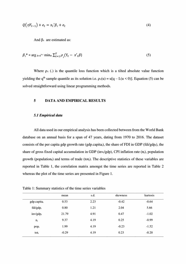
All data used in our empirical analysis has been collected between from the World Bank

database on an annual basis for a span of 47 years, dating from 1970 to 2016. The dataset

consists of the per capita gdp growth rate (gdp.capitat), the share of FDI in GDP (fdi/gdpt), the

share of gross fixed capital accumulation in GDP (invt/gdp), CPI inflation rate (πt), population

growth (populationt) and terms of trade (tott). The descriptive statistics of these variables are

reported in Table 1, the correlation matrix amongst the time series are reported in Table 2

whereas the plot of the time series are presented in Figure 1.

Table 1: Summary statistics of the time series variables

mean s.d. skewness kurtosis

gdp.capitat 0.53 2.23 -0.42 -0.64

fdi/gdpt 0.80 1.21 2.04 5.66

inv/gdpt 21.79 4.91 0.47 -1.02

t 9.37 4.19 0.25 -0.99

popt 1.99 4.19 -0.23 -1.52

tott -0.29 4.19 0.23 -0.20

Note: Authors own computation

Table 2: Correlation matrix of the time series variables

gdp.capitat fdi/gdpt inv/gdpt t popt tott

gdp.capitat 1.00 0.26 -0.11 0.43 -0.28 0.04

fdi/gdpt 1.00 -0.31 -0.43 -0.58 -0.09

inv/gdpt 1.00 0.44 0.70 -0.37

t 1.00 0.63 -0.18

popt 1.00 -0.36

tott 1.00

Note: Authors own computation

Figure 1: Time series plot of the variables

As can be observed from the summary of descriptive statistics reported in Table 1, the

skewness and kurtosis statistics particularly hint that the time series may not be normally

-5

-4

-3

-2

-1

0

1

2

3

4

5

1970 1977 1984 1991 1998 2005 2012

gdpcapita

-1

0

1

2

3

4

5

6

1970 1977 1984 1991 1998 2005 2012

fdi

14

16

18

20

22

24

26

28

30

32

34

1970 1977 1984 1991 1998 2005 2012

gfdi

0

2

4

6

8

10

12

14

16

18

20

1970 1977 1984 1991 1998 2005 2012

inf

-10

-8

-6

-4

-2

0

2

4

6

8

10

1970 1977 1984 1991 1998 2005 2012

tot

0,8

1

1,2

1,4

1,6

1,8

2

2,2

2,4

2,6

2,8

1970 1977 1984 1991 1998 2005 2012

pop

distributed. This observation provides a genuine case for the use of quantile regression over

traditional OLS estimates. Also note some of the linear dependences between the variables as

depicted by the correlation matrices presented in Table 2, are in contradiction to what is dictated

by conventional growth theory, for instance, the negative relationship between FDI and per

capita GDP growth as well as the positive correlation between inflation and per capital GDP

growth. This further provides a plausible reason for further econometric analysis that would

paint a broader picture than that presented by linear estimates. In this sense, quantile regression

present a suitable alternative methodology.

5.2 Unit root tests

Before we can estimate our empirical QR model, we first perform unit root and

cointegration tests in order to avoid the possibility of spurious regressions in our empirical

estimates. The concept of a unit root within a time series can be demonstrated by specifying

the following autoregressive (AR) model of a time series, yt, i.e.

𝑦𝑡 = 𝛼𝑦𝑡−1 + 𝑒𝑡 (6)

Where et ~ iid. From regression (6)., the series yt is said to be stationary if α < 1 and

the series contains a unit root process if α = 1. Dickey and Fuller (1979) extend equation (5) to

accommodate ARMA structure through the following test regression:

𝑦𝑡 = 𝛽′𝐷𝑡 + 𝑦𝑡−1 + σ 𝑗𝑝𝑖=1 ∆𝑦𝑡−𝑖 + 𝑒𝑡 (7)

Where the vector Dt is a vector of deterministic trends. The hypotheses tested are

formally given as:

H0: = 1, yt ~ I(1) (8)

H1: = 1, yt ~ I(0) (9)

And the test statistic used to test the above hypothesis is computed as:

𝐴𝐷𝐹=1 = ∗ሶ −1𝑆𝐸(∗ሶ ) (10)

Where * and SE(*) are the least squares estimate of and the standard error estimate,

respectively. The critical values of the ADF tests statistics are reported in MacKinnon (1996).

We perform the unit root tests on the levels as well as on the first differences of our time series

variables and report the results in Table 3 below. Note that the unit root tests are performed

with i) no constant, ii) a constant and ii) a trend, with the maximum lag used in the ADF test

based on the modified AIC (MAIC).

Table 3: ADF unit root tests results

time series levels first differences

drift trend drift trend

gdp.capitat 0.14 -3.51* -5.83*** -5.83***

fdi/gdpt -0.46 -4.47*** -3.15** -3.15

inv/gdpt -2.45 -5.43*** -2.93* -2.93

t -2.52 -4.11** -2.84* -2.84

popt -1.22 -1.52 -5.40*** -5.37***

tott -0.61 -0.31 -1.73* -1.73

Notes: “***”, “**”,”*” denote the 1%, 5% and 10% significance levels, respectively.

Based on the reported results, all observed time series fail to reject the unit root null in

the levels of the variables when the tests are performed with a drift. However, when a trend is

included the unit root null is rejected for the per capita gdp (10% statistical significance), FDI

(significant at all critical levels), domestic investment (significant at all critical levels) and

inflation (5% statistical significance) variables. In their first differences, all the time series

reject the unit root null at significance levels of at least 10 percent when the test is conducted

with a drift. When performed with a trend, only the gdp.capita and population variables reject

the unit root null hence rendering the results of the unit root tests performed with a trend as

being ambiguous. We therefore consider the results of the test run with only a drift and declare

that all series are first difference I(1) variables, a condition which is indicative of cointegration

amongst the time series. We thus formally test for cointegration relations within the series in

the next section of the paper.

5.3 Cointegration tests

The concept of cointegration originated in the seminar work of Engle and Granger

(1987). According to these authors, a pair of time series variables can be said to be cointegrated

if the variables are mutually first difference variables and collectively produce a stationary

error term. Their theorem particularly notes that such a condition will ensure that there exists

a singular cointegration vector between the time series over the long-run. Johansen (1991)

extend upon Engle and Granger (1987) by allowing for multiple cointegration vectors or

relations for a vector of time series. In particular, Johansen (1991) devised two likelihood ratio

tests for cointegration. The first, the lambda-maximum test, is based on the log-likelihood ratio

Ln[Lmax(r)/Lmax(r+1) and is conducted sequentially for r = 0, 1, …, k-1. The second test, the

trace test, is based on the log-likelihood ratio Ln[Lmax(r)/Lmax(k) and is conducted

sequentially for r = k-1, …, 1, 0. Seeing that we have previously found our time series to be

difference stationary variables, we are enabled to test for multivariate cointegration vectors

amongst the time series. The results of Johansen’s (1991) cointegration tests as performed on

our time series are found in Table 3 and based on the obtained test statistics for both Eigen and

trace cointegration tests, we are compelled to render that there are two cointegration vectors

amongst the observed variables.

Table 4: Johansen’s test for cointegration

Rank Eigen statistic p-value Trace statistic p-value

0 175.04 0.00*** 75.40 0.00***

1 99.64 0.00*** 38.74 0.00***

2 60.90 0.00*** 38.15 0.00***

3 22.75 0.27 11.87 0.57

4 10.89 0.22 8.79 0.31

5 2.09 0.15 2.09 0.15

Notes: “***”, “**”,”*” denote the 1%, 5% and 10% significance levels, respectively.

5.4 QAR regression estimation results

The quantile regression estimates of our empirical model are reported in Tables 5, and

has been executed for nine quantiles (i.e. 10th quantile, 20th quantile, 30th quantile, 40th quantile,

50th quantile, 60th quantile, 70th quantile, 80th quantile and 90th quantile). The plots of

coefficients from the quantile functions for each of the time series regressors are provided in

Figure 2. Also note that for comparative sake, the OLS estimates of the long-run regression are

also reported in Table 1. As can be observed, the OLS estimates indicate a surprisingly negative

and significant coefficient on FDI and yet a produces a positive and significant coefficient on

domestic investment. Note that these results concur with that obtained from the study of

Mazenda (2014) for South Africa and Rahman (2015) for Bangladesh, albeit using different

econometric techniques. Other results reported in Table 1 include a correct negative yet

insignificant coefficient on inflation, a negative and insignificant coefficient on population and

a negative and significant coefficient on terms of trade.

However, the estimates from our quantile regression indicate that the OLS esteems may

be depicting an incomplete picture of the actual relationship. For instance, for the FDI variable,

we find a negative and significant estimates at the 10th and 40th quantile whereas at the

remaining quantiles, the coefficients are negative and insignificant. The insignificant effect of

FDI on economic growth has been previously found in the studies of Tang (2015) for EU

countries, Naguibi (2002) for Argentina, Chakraborty and Basu (2002) for India, Khaliq and

Noy (2007), Herzer et. al. (2008) for developing countries as well as Esso (2010) for SSA

countries. Concerning the domestic investment, we note positive and significant impact of

domestic investment on economic growth at all quantiles with the effect being more

pronounced as one moves up the quantiles. In turning to the inflation variable, we note a

negative and highly significant coefficients at the lower quantiles (i.e. 10th, 20th, 30th and 40th)

as well as at the 90th quantile whilst at other quantiles the coefficients turn insignificant. The

coefficients on the population variable remain insignificant throughout the quantiles albeit

being positive up to the 30th quantile and turn negative thereafter. Finally, the quantile

coefficient estimates on the terms of trade variable are more puzzling, being negative and

significant at the 10th and 40th quantiles, positive at the 20th quantile and turning positive and

insignificant at all other quantiles.

Table 5: QAR regression estimates on original time series

q fdi/gdpt inv/gdpt t popt tott

estimate p-

value

estimate p-

value

estimate p-

value

estimate p-

value

estimate p-

value

ols -0.43 0.03** 0.36 0.00*** -0.06 0.74 -0.24 0.15 -1.57 0.15

0.1 -0.41 0.00*** 0.19 0.00*** -0.23 0.00*** 0.21 0.42 -0.12 0.00***

0.2 -0.03 0.26 0.17 0.00*** -0.36 0.00*** 0.01 0.79 0.40 0.00***

0.3 -0.08 0.60 0.17 0.02** -0.29 0.04** 0.48 0.53 -0.10 0.32

0.4 -0.18 0.02** 0.22 0.00*** -0.20 0.00*** -0.14 0.64 -0.15 0.00***

0.5 -0.52 0.27 0.39 0.05** 0.10 0.77 -2.24 0.32 -0.31 0.29

0.6 -0.52 0.26 0.39 0.04** 0.10 0.76 -2.24 0.31 -0.31 0.28

0.7 -0.50 0.15 0.41 0.00*** -0.10 0.67 -1.73 0.28 -0.19 0.36

0.8 -0.24 0.33 0.38 0.00*** -0.24 0.20 -1.09 0.34 -0.13 0.39

0.9 -0.24 0.18 0.38 0.00*** -0.24 0.08* -1.09 0.20 -0.13 0.24

Notes: “***”, “***”, “*” represent the 1%, 5% and 10% significance level, respectively.

Figure 2: Plots of coefficients from different quantiles

5.5 Sensitivity analysis

Notwithstanding, the encouraging results obtained from our initial quantile estimates,

we feel it is important to perform sensitivity analysis on our estimated regressions. A significant

yet often overlooked factor that would distort the FDI-growth relationship overt time would be

the structural break caused by the 2007 global financial crisis. Thus, we conduct our sensitivity

-2

-1,5

-1

-0,5

0

0,5

1

0 0,2 0,4 0,6 0,8 1

tau

Coefficient on fdi

Quantile estimates with 95% band

OLS estimate with 95% band 0

0,1

0,2

0,3

0,4

0,5

0,6

0,7

0,8

0 0,2 0,4 0,6 0,8 1

tau

Coefficient on gfdi


OLS estimate with 95% band

-0,8

-0,6

-0,4

-0,2

0

0,2

0,4

0,6

0,8

1

0 0,2 0,4 0,6 0,8 1

tau

Coefficient on inf


OLS estimate with 95% band-1

-0,8

-0,6

-0,4

-0,2

0

0,2

0,4

0 0,2 0,4 0,6 0,8 1

tau

Coefficient on tot



-8

-7

-6

-5

-4

-3

-2

-1

0

1

2

3

0 0,2 0,4 0,6 0,8 1

tau

Coefficient on pop



analysis as means of ensuring that our estimates are not biased, we segregate our data into two

sub-periods corresponding to the pre-crisis (1970-2006) and post-crisis (2007-2016) periods

and performed our empirical quantile estimates on the theses sub-samples. In being aware of

the danger posed by the low number of observations particular associated with post-crisis

period, we interpolate our data from annual to quarterly frequencies as a means of increasing

the observations numbers available for empirical use. The results of this empirical exercise are

reported in Table 6 with the associated plots of coefficients from the quantile functions for the

pre-crisis and post-crisis periods are plotted in Figures 3 and 4, respectively.

In quickly browsing through the OLS estimates, we note that all obtained coefficients

are insignificant in both sub-sample periods with the exception of the inflation coefficient in

the pre-crisis which produces the correct negative and significant regression estimate. We also

summarize the findings of our quantile estimates as follows. For the FDI variable, we note that

coefficient estimate is negative and significant at the 60th and 80th quantile and in the 10th, 20th

and 90th quantiles in the post-crisis. We also find significant positive coefficient estimate on

the domestic investment variable at the 10th and 90th quantile for both pre-and-post crisis

periods, the 40th, 60th, 70th and 80th quantile in the pre-crisis periods and the 20th quantile in the

post-crisis period. Inflation is also found to have a negative and significant in both sub-sample

periods at the 90th quantile whereas the coefficient estimates are negative and significant at all

other quantiles for the pre-crisis periods whereas they turn negative and insignificant in the

post-crisis data. On the other hand, population is negative and significant at the 60th and 80th

quantiles for the pre-crisis period and at the 10th, 20th and 90th quantiles in the post-crisis

whereas the remaining coefficient estimates as negative and insignificant. Lastly, terms of trade

coefficients are negative and significant at the 60th and 80th quantiles in the pre-crisis and at the

10th, 20th and 90th quantile for the post-crisis period. All-in-all, we observe a change in

regression results when account for the global financial crisis, note only for the quantile

regressions but also for the OLS estimates.

Table 6: QAR regression estimates on logs of variables

q fdi/gdpt inv/gdpt t popt tott

estimate p-

value

estimate p-

value

estimate p-

value

estimate p-

value

estimate p-

value

ols Pre-

crisis

0.33 0.21 0.13 0.22 -0.24 0.00*** -0.15 0.89 0.05 0.60

Post-

crisis

-1.06 0.67 1.19 0.48 -0.53 0.61 -12.30 0.49 -0.20 0.60

0.1 Pre-

crisis

-0.03 0.71 0.17 0.00*** -0.36 0.00*** 0.40 0.30 0.01 0.94

Post-

crisis

-4.95 0.00*** 2.49 0.00*** 0.07 0.84 -29.54 0.00*** -0.57 0.00***

0.2 Pre-

crisis

-0.03 0.90 0.17 0.12 -0.36 0.09* 0.40 0.73 0.01 0.98

Post-

crisis

-4.95 0.00*** 2.49 0.02** 0.07 0.88 -29.54 0.00*** -0.57 0.02**

0.3 Pre-

crisis

-0.03 0.90 0.17 0.11 -0.36 0.08* 0.40 0.72 0.01 0.98

Post-

crisis

-0.61 0.62 1.02 0.24 -0.40 0.44 -11.23 0.23 -0.25 0.22

0.4 Pre-

crisis

-0.08 0.48 0.17 0.02** -0.29 0.02** 0.48 0.43 -0.10 0.21

Post-

crisis

0.37 0.73 0.68 0.36 -0.50 0.29 -7.10 0.37 -0.18 0.30

0.5 Pre-

crisis

-0.08 0.74 0.17 0.15 -0.29 0.19 0.48 0.71 -0.10 0.53

Post-

crisis

-0.33 0.85 1.31 0.28 -0.85 0.26 -13.11 0.30 -0.13 0.63

0.6 Pre-

crisis

-0.76 0.00*** 0.50 0.00*** 0.32 0.00*** -3.74 0.00*** -0.40 0.00***

Post-

crisis

-1.35 0.54 2.22 0.17 -1.37 0.17 -21.88 0.20 -0.05 0.89

0.7 Pre-

crisis

-0.19 0.35 0.30 0.02** -0.61 0.01** 0.70 0.50 0.05 0.68

Post-

crisis

-1.35 0.54 2.22 0.17 -1.37 0.17 -21.88 0.20 -0.05 0.89

0.8 Pre-

crisis

-0.19 0.01** 0.30 0.00*** -0.61 0.00*** 0.70 0.03** 0.05 0.14

Post-

crisis

-1.38 0.48 2.25 0.12 -1.32 0.13 -22.36 0.14 -0.05 0.87

0.9 Pre-

crisis

-0.19 0.36 0.30 0.02** -0.6 0.01** 0.70 0.50 0.05 0.69

Post-

crisis

-1.38 0.00*** 2.25 0.00*** -1.32 0.00*** -22.36 0.00*** -0.05 0.08*

Notes: “***”, “***”, “*” represent the 1%, 5% and 10% significance level, respectively.

Figure 3: Plots of coefficients from different quantiles (pre-crisis)

-1,4

-1,2

-1

-0,8

-0,6

-0,4

-0,2

0

0,2

0,4

0,6

0,8

0 0,2 0,4 0,6 0,8 1

tau

Coefficient on fdi


OLS estimate with 95% band-0,1

0

0,1

0,2

0,3

0,4

0,5

0,6

0,7

0,8

0 0,2 0,4 0,6 0,8 1

tau

Coefficient on gfdi



-1,2

-1

-0,8

-0,6

-0,4

-0,2

0

0,2

0,4

0,6

0 0,2 0,4 0,6 0,8 1

tau

Coefficient on inf



-0,6

-0,4

-0,2

0

0,2

0,4

0,6

0 0,2 0,4 0,6 0,8 1

tau

Coefficient on tot



-6

-5

-4

-3

-2

-1

0

1

2

3

4

5

0 0,2 0,4 0,6 0,8 1

tau

Coefficient on pop



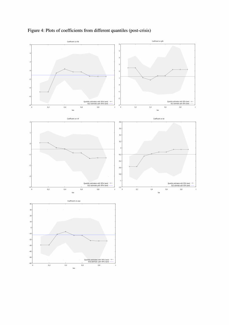
Figure 4: Plots of coefficients from different quantiles (post-crisis)

-8

-6

-4

-2

0

2

4

6

0 0,2 0,4 0,6 0,8 1

tau

Coefficient on fdi


OLS estimate with 95% band-3

-2

-1

0

1

2

3

4

5

6

0 0,2 0,4 0,6 0,8 1

tau

Coefficient on gfdi



-4

-3

-2

-1

0

1

2

0 0,2 0,4 0,6 0,8 1

tau

Coefficient on inf



-1

-0,8

-0,6

-0,4

-0,2

0

0,2

0,4

0,6

0,8

0 0,2 0,4 0,6 0,8 1

tau

Coefficient on tot



-60

-50

-40

-30

-20

-10

0

10

20

30

40

0 0,2 0,4 0,6 0,8 1

tau

Coefficient on pop



6 CONCLUSION

Much debate has been cast on the relationship between FDI and growth more

prominently so during the post 2008-recession era. It is widely believed that FDI is an

important component in assisting the world economy recovering from the recessionary period,

more specifically so for developing regions. We contribute to the on-going literature by

presenting an empirical analysis of the effects of FDI on growth in South Africa, one of the

largest recipients of FDI in the Sub-Saharan Africa (SSA) region. In differing from previous

South African case studies we use quantile regression approach as opposed to restrictive OLS

technique and carry out our analysis using data collected from 1970 to 2016. As part of our

sensitivity analysis, we accounted for the global financial crisis as a break period and perform

a comparative analysis thereafter.

Concerning the FDI-growth relationship, our results indicate that FDI negatively affects

economic growth welfare at lower extreme quantiles more prominently so during the post-

crisis period. At other levels, FDI insignificantly influences welfare. Conversely, we find that

domestic investment positively affects per capita GDP growth in a majority of quantiles

regardless of the observed sample period. Collectively, a plausible policy implication which

can be drawn from our analysis is that FDI may be crowding out domestic investment in the

aftermath of the global financial crisis via a displacement effect. Our results thus caution

policymakers to not only dedicate efforts towards attracting more levels of FDI but should

more importantly focus on developing strategies and channels through which FDI can be

directed at improving economic welfare in South Africa. Identifying the channels through

which FDI can possible influence economic welfare without crowding out domestic investment

would thus pose as the main challenge to policymakers. However, given the limited scope of

this current study, this subject matter can be empirically reserved for future research analysis

using appropriate estimation technique.

REFERENCES

Adams S. (2009), “Foreign direct investment, domestic investment and economic growth in

Sub-Saharan Africa”, Journal of Policy Modeling, 31, 939-949.

Alfaro L. (2003), “Foreign direct investment and growth: Does the sector matter”, Harvard

Business School, 1-31.

Alfaro L. and Chen M. (2011), “Surviving the global financial crisis: Foreign ownership and

establishment performance”, NBER Working Paper No. 17141, June.

Alfaro L., Chanda A., Kalemli-Ozcan S. and Sayek S. (2004), “FDI and economic growth: The

role of local financial markets”, Journal of International Economics, 64, 89-112.

Agrawal G. (2015), “Foreign Direct Investment and Economic Growth in BRICS Economies:

A panel data analysis”, Journal of Economics, Business and Management, 3(4), 421-424.

Bengoa M. and Sanchez-Robles B. (2003), “Foreign direct investment, economic growth and

growth: New evidence from Latin America”, European Journal of Political Economy, 19(3),

529-545.

Borensztein E., de Gregorio J. and Lee J. (1998), “How does FDI affect economic growth?”,

Journal of International Economics, 45(1), 115-135.

Buckley P. and Casson M. (1976), “The future of the multinational enterprises”, MacMillan,

London.

Chakraborty C. and Basu P.(2002), “Foreign direct investment and growth in India: A

cointegration approach”, Applied Economics, 34, 1.61-1073.

Choe J. (2003), “Do foreign direct investment and gross domestic investment promote

growth?”, Review of Development Economics, 7(1), 44-57.

Coase R. (1937), “The nature of the firm”, Economica, 4, 386-405.

Dias M., Dias J. and Hirata, J. (2014), “Foreign Direct Investment in Brazil: The effects of

productivity and aggregate consumption”, Journal of Stock and Forex Trading, 3(127), 59-73.

Dickey D. and Fuller W. (1979), “Distribution of the estimators for autoregressive time series

with a unit root”, Journal of the America Statistical Association, 74(366), 427-431.

Domar D.E. (1946), “Capital expansion, rate of growth and employment”, Econometrica,

14(2), 137-147.

Dunning J (1973), “The Determinants of International Production”, Oxford Economic

Papers, 25, 289-336.

Engle R. and Granger C. (1987), “Co-integration and error correction: Representation,

estimation and testing”, Econometrica, 55(2), 251-276.

Esso L. (2010), “Long-run relationship and causality between foreign direct investment and

growth: Evidence from ten African countries”, International Journal of Economics and

Finance, 2(2), 168-177.

Fedderke J. and Romm T. (2006), “Growth impact and determinants of foreign direct

investment into South Africa: 1956-2003”, Economic Modleing, 23, 738-760.

Gupta K. and Garg I. (2015), “Foreign Direct Investment and Economic Growth in India: An

Econometric Approach”, Journal of Management Sciences and Technology, 2(3), 6-14.

Hansen G. and Rand J. (2006), “On the causal links between FDI and growth in developing

countries”, The World Economy, 29, 1-21.

Harrod R.F. (1939), “An essay in dynamic theory”, The Economic Journal, 49(193), 14-33.

Herzer D., Klasen S., Nowak-Lehmann F. (2008), “In search of FDI-led growth in developing

countries: The way forward”, Economic Modeling, 25, 793-810.

Hong L. (2014), “Does and how does FDI promote the economic growth? Evidence from

dynamic panel data of prefecture city in China”, IERI Procedia, 6, 57-62.

Hymer S. (1970), “The Efficiency (Contradictions) of Multinational Corporations”, American

Economic Review Papers and Proceedings, 60, 441-48

Hymer, S. (1976), “The International Operations of National Firms: A Study of Direct

Foreign Investment”, Boston: MIT Press.

Johansen S. (1991), “Estimation and hypothesis testing of cointegration vectors in Gaussian

vector autoregressive models”, Econometrica, 59(6), 1551-1580.

Jugurnath B., Chuckun N. and Fauzel S. (2016), “Foreign direct investment and economic

growth in Sub-Saharan Africa: An empirical study”, Theoretical Economic Letters, 6, 798-807.

Keho Y. (2015), “Foreign direct investment, exports and economic growth: Some African

evidence”, Journal of Applied Economics and Business Research, 5(4), 209-219.

Khaliq A. and Noy I. (2007), “Foreign Direct Investment and Economic Growth: Empirical

Evidence from Sectoral Data in Indonesia”, Department of Economics, University of Hawaii

at Manoa, Working Paper No. 2007-29, March.

Koenker R. and Bassett G. (1978), “Regression Quantiles”, Econometrica, 46(1), 33-50.

Koenker R. and Hallock K. (2001), “Quantile regression”, Journal of Economic Perspectives,

15(4), 143-156.

Kumar R. (2014), “FDI and Economic Growth – A Case Study of India”, International

Conference on Business, Law and Corporate Social Responsibility, October (1-2), 107-110.

Kindelberger C. (1969), “American Business Abroad: Six Lectures on Direct Investment”, New

Haven: Yale University Press.

Knickerbocker F. (1973), “Oligopolistic reaction and multinational enterprise”, Thunderbird

International Business Review, 15(2), 7-9.

Leitao N. and Rasekhi S. (2013), “The impact of foreign direct investment on economic

growth: the Portuguese experience”, Theoretical and Applied Economics, 20(1), 51-62..

Li X. and Liu X. (2005), “Foreign direct investment and economic growth: An increasingly

endogenous relationship”, World Development, 33(3), 393-407.

Lucas R. (1988), “On the mechanics of economic development”, Journal of Monetary

Economics, 22, 3-42.

MacKinnon J. (1996), “Numerical distribution functions for unit root and cointegration tests”,

Journal of Applied Econometrics, 11, 601-618.

Masipa T. (2014), “The impact of foreign direct investment on economic growth and

employment in South Africa: A time series analysis”, Mediterranean Journal of Social

Sciences, 5(25), 18-27.

Matenyo J., Osoro N., Muwanga J. and Bbale J. (2017), “Foreign direct investment and

economic growth in Sub Saharan Africa: Do institutions and human capital matter?”,

International Journal of Social Science and Economic Research, 2(5), 3461-3489.

Mazenda A. (2014), “The effect of foreign direct investment on economic growth: Evidence

from South Africa”, Mediterranean Journal of Social Sciences, 5(10), 95-108.

Moosa I. (2015), “Theories of foreign direct investment: Diversity and implications for

empirical testing”, Transnational Corporations Review, 7(3), 397-315.

Morck R. and Yeung B. (1992), “Internalization: An event study”, Journal of International

Economics, 33, 41-56.

Moudatsou A. (2003), “Foreign Direct Investment and Economic Growth in the European

Union”, Journal of Economic Integration, 18(4), 689-707.

Moudatsou A. and Kyrkilis D. (2011), “FDI and economic growth: Causality for the EU and

ASEAN”, Journal of Economic Integration, 26(3), 554-577.

Naguibi R. (2002), “The effects of privatization and foreign direct investment on economic

growth in Argentina”, The Journal of International Trade and Economic Development, 21(1),

51-82.

Najaf K. and Najaf R. (2016), “Importance of FDI on the growth of Pakistan and Afghanistan”,

Middle-East Journal of Scientific Research, 24(5), 1738-1742.

Nair-Reichert U. and Weinhold D. (2001), “Causality tests for cross-country panels: A new

look at FDI and economic growth in developing countries”, Oxford Bulletin of Economics and

Statistics, 63(2), 153-171.

Nayak D. and Choudhury R. (2014), “A selective review of foreign direct investment theories”,

ARTNet Working Paper Series No. 143, March.

Nayyar R. (2014), “Traditional and modern theories of FDI”, International Journal of Business

and Management Innovation, 3(6), 23-26.

Naz S., Sabir G. and Ahmed M. (2015), “Impact of Foreign Direct Investment on Economic

Growth: Empirical Results from Pakistan”, Journal of Poverty, Investment and Development,

12, 101-105.

Pandya V. and Sisombat S. (2017), “Impacts of Foreign Direct Investment on Economic

Growth: Empirical Evidence from Australian Economy”, Interntioanl Journal of Economics

and Finance, 9(5), 121-131.

Rahman A. (2015), “Impact of foreign direct investment of economic growth: Empirical

evidence from Bangladesh”, International Journal of Economics and Finance, 7(2), 1-12.

Romer P. (1986), “Increasing returns and long-run growth”, Journal of Political Economy, 94,

1002-1037.

Roy G. and Van den Berg H. (2006), “Foreign Direct Investment and Economic Growth: A

Time-Series Approach”, Global Economy Journal, 6(1), 1-19.

Rudy T. (2012), “Foreign direct investment and growth: Theory, evidence and lessons for

Egypt”, Journal of International Business Research, 11(1), 1-14.

Sakyi D. and Egyir J. (2017), “Effects of trade and FDI on economic growth in Africa: an

empirical investigation”, Transnational Corporations Review, 9(2), 66-87.

Seetanah B. and Khadaroo A. (2007), “Foreign direct investment and growth: New evidence

from Sub-Saharan countries”, Economic development in Africa 2007: CSAE conference.

Seyoum M., Wu R. and Lin J. (2015), “Foreign direct investment and economic growth: The

case of developing African economies”, Social Indicators Research, 122(1), 45-64.

Solow R.M. (1965), "A contribution to the theory of economic growth", Quarterly Journal of

Economics, 70(1), 65-94.

Solow R.M. (1994), "Perspectives on growth theory", Journal of Economic Perspectives, 66-

67(1-4), 400-410.

Sridharan P., Vijayakumar N. and Chandra S. (2009), “Causal Relationship between Foreign

Direct Investment and Growth: Evidence from BRICS Countries”, International Business

Research, 2(4), 198-203.

Sunde T. (2017), “Foreign direct investment, exports and economic growth: ADRL and

causality analysis for South Africa”, Research in International Business and Finance, 41,

434-444.

Tang D. (2015), “Has the foreign direct investment boosted economic growth in European

Union countries?”, The Journal of International and Global Economic Studies, 8(1), 21-50.

UNCTAB (2013), “World investment report: Foreign direct investment and the challenge of

development”, New York and Genova: United Nations.

Velnampy T., Achchuthan S. and Kajananthan R. (2013), “Foreign Direct Investment and

Economic Growth: Evidence from Sri Lanka”, International Journal of Business and

Management, 9(1), 140-148.

Williamson O. (1979), “Transaction-Cost Economics: The Governance of Contractual

Relations‟, Journal of Law and Economics, 22(2), 233-61.

Zhang K. (2001), “How does foreign direct investment affect economic growth in China?”,

Economics of transition, 9(3), 679-693.

Zhang K. (2006), “Foreign direct investment and economic growth: A panel data study for

1992-2004”, Conference of WTO, China and Asian Economies, University of International

Business and Economics, Beijing.

Documents

The FDI-growth nexus in South Africa: A re-examination