The Fast Fourier Transform Andreas Klappenecker

Motivation

There are few algorithms that had more impact on modern society than the fast Fourier transform and its relatives.

The applications of the fast Fourier transform touch nearly every area of science and engineering in some way.

For example, it changed medicine by enabling magnetic resonance imaging. It sparked a revolution in the music industry. It even finds uses in applications such as the fast multiplication of large integers.

A Brief History

Gauss (1805, 1866). Used the FFT in calculations in astronomy.

Danielson-Lanczos (1942). Gave an efficient algorithm, but low impact as digital computer were just emerging.

Cooley-Tukey (1965). Rediscovered and popularized FFT. The importance was immediately recognized, and this is one of the most widely cited papers in science and engineering.

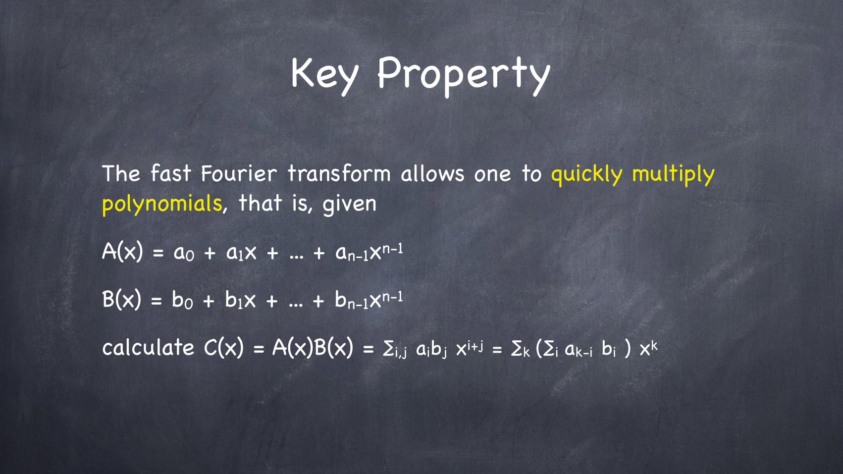
Key Property

The fast Fourier transform allows one to quickly multiply polynomials, that is, given

A(x) = a0 + a1x + ... + an-1xn-1

B(x) = b0 + b1x + ... + bn-1xn-1

calculate C(x) = A(x)B(x) = ∑i,j aibj xi+j = ∑k (∑i ak-i bi ) xk

Representations of Polynomials

Coefficient Representation

A polynomial

A(x) = a0 + a1x + ... + an-1xn-1

can be represented in various ways. The most common way is to specify its coefficients (a0, a1, ... , an-1); this is called the coefficient representation.

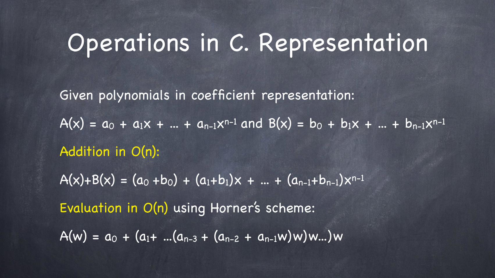
Operations in C. Representation

Given polynomials in coefficient representation:

A(x) = a0 + a1x + ... + an-1xn-1 and B(x) = b0 + b1x + ... + bn-1xn-1

Addition in O(n):

A(x)+B(x) = (a0 +b0) + (a1+b1)x + ... + (an-1+bn-1)xn-1

Evaluation in O(n) using Horner’s scheme:

A(w) = a0 + (a1+ ...(an-3 + (an-2 + an-1w)w)w...)w

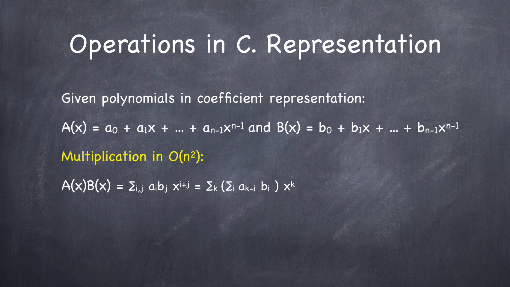
Operations in C. Representation

Given polynomials in coefficient representation:

A(x) = a0 + a1x + ... + an-1xn-1 and B(x) = b0 + b1x + ... + bn-1xn-1

Multiplication in O(n2):

A(x)B(x) = ∑i,j aibj xi+j = ∑k (∑i ak-i bi ) xk

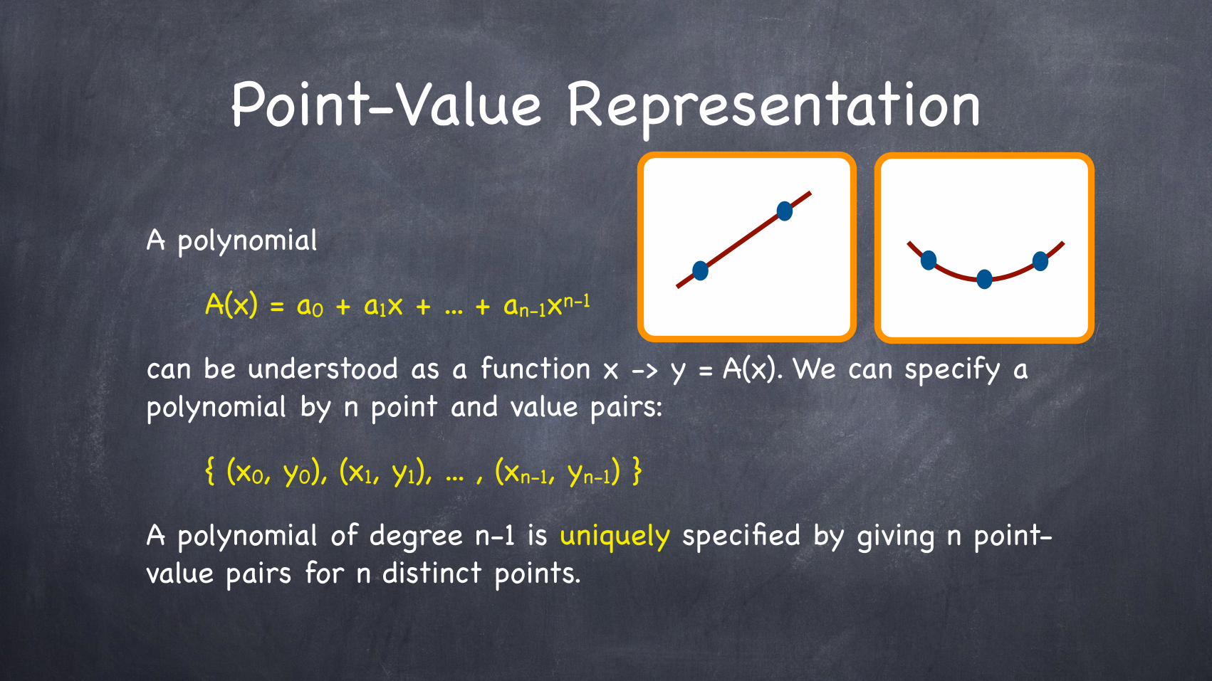
Point-Value Representation

A polynomial

A(x) = a0 + a1x + ... + an-1xn-1

can be understood as a function x -> y = A(x). We can specify a polynomial by n point and value pairs:

{ (x0, y0), (x1, y1), ... , (xn-1, yn-1) }

A polynomial of degree n-1 is uniquely specified by giving n point-value pairs for n distinct points.

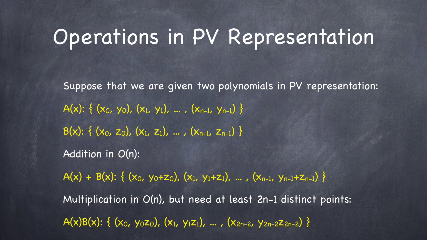
Operations in PV Representation

Suppose that we are given two polynomials in PV representation:

A(x): { (x0, y0), (x1, y1), ... , (xn-1, yn-1) }

B(x): { (x0, z0), (x1, z1), ... , (xn-1, zn-1) }

Addition in O(n):

A(x) + B(x): { (x0, y0+z0), (x1, y1+z1), ... , (xn-1, yn-1+zn-1) }

Multiplication in O(n), but need at least 2n-1 distinct points:

A(x)B(x): { (x0, y0z0), (x1, y1z1), ... , (x2n-2, y2n-2z2n-2) }

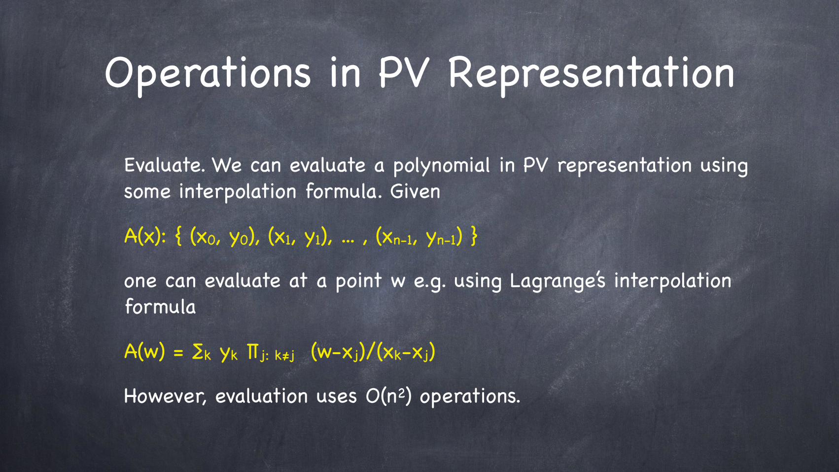
Operations in PV Representation

Evaluate. We can evaluate a polynomial in PV representation using some interpolation formula. Given

A(x): { (x0, y0), (x1, y1), ... , (xn-1, yn-1) }

one can evaluate at a point w e.g. using Lagrange’s interpolation formula

A(w) = ∑k yk ∏j: k≠j (w-xj)/(xk-xj)

However, evaluation uses O(n2) operations.

Tradeoffs

Coefficient

Representation

O(n2)

Multiply

O(n)

Evaluate

Point-value O(n) O(n2)

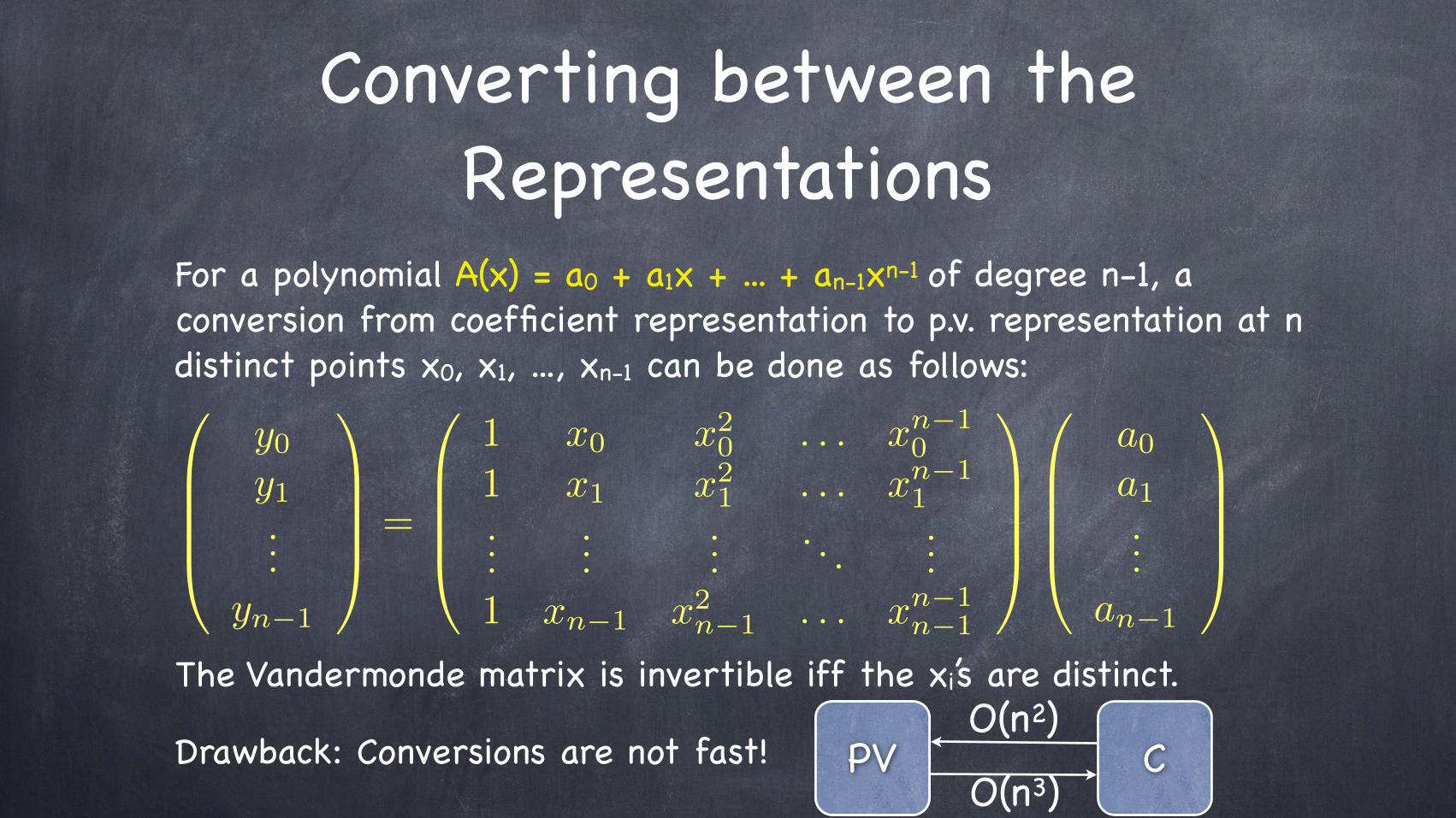
Converting between the Representations

For a polynomial A(x) = a0 + a1x + ... + an-1xn-1 of degree n-1, a conversion from coefficient representation to p.v. representation at n distinct points x0, x1, ..., xn-1 can be done as follows:

The Vandermonde matrix is invertible iff the xi’s are distinct.

Drawback: Conversions are not fast!

0

BBB@

y0y1...

yn�1

1

CCCA=

0

BBB@

1 x0 x20 . . . xn�1

0

1 x1 x21 . . . xn�1

1...

......

. . ....

1 xn�1 x2n�1 . . . xn�1

n�1

1

CCCA

0

BBB@

a0a1...

an�1

1

CCCA

PV CPVO(n2)

O(n3)

The Fast Fourier Transform II Andreas Klappenecker

Divide-and-Conquer

Motivation

We can speed up the evaluation by choosing suitable points x0,...,xn-1 that have sufficient structure so that we can reuse computational results.

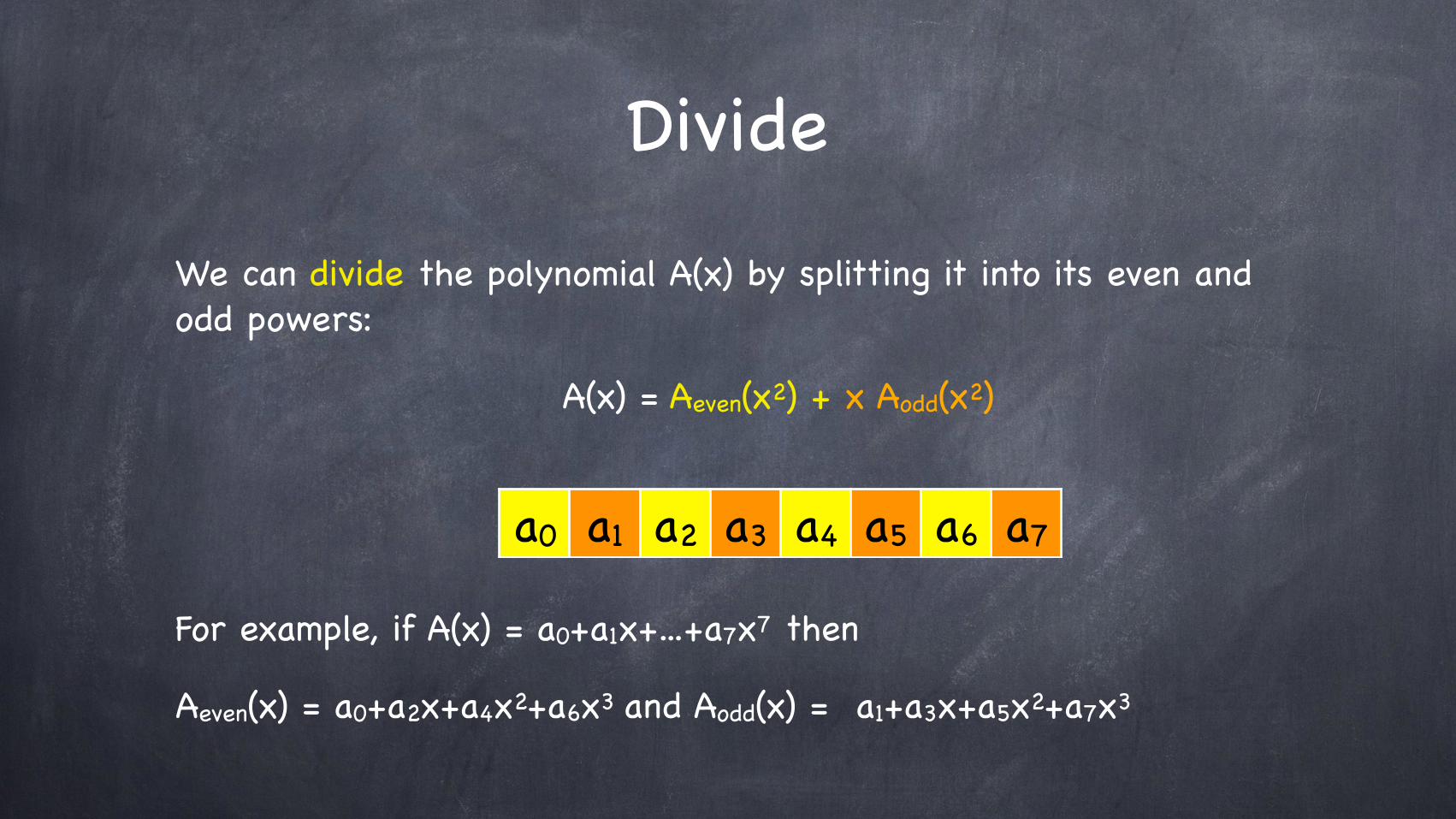
Divide

We can divide the polynomial A(x) by splitting it into its even and odd powers:

A(x) = Aeven(x2) + x Aodd(x2)

For example, if A(x) = a0+a1x+...+a7x7 then

Aeven(x) = a0+a2x+a4x2+a6x3 and Aodd(x) = a1+a3x+a5x2+a7x3

a0 a1 a2 a3 a4 a5 a6 a7

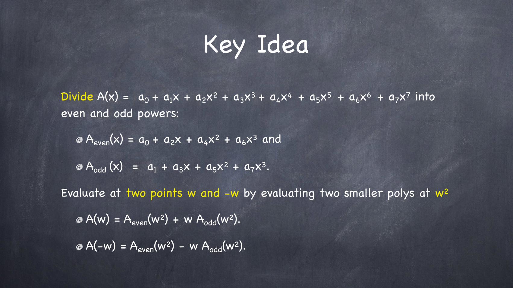
Key Idea

Divide A(x) = a0 + a1x + a2x2 + a3x3 + a4x4 + a5x5 + a6x6 + a7x7 into even and odd powers:

Aeven(x) = a0 + a2x + a4x2 + a6x3 and

Aodd (x) = a1 + a3x + a5x2 + a7x3.

Evaluate at two points w and -w by evaluating two smaller polys at w2

A(w) = Aeven(w2) + w Aodd(w2).

A(-w) = Aeven(w2) - w Aodd(w2).

Example

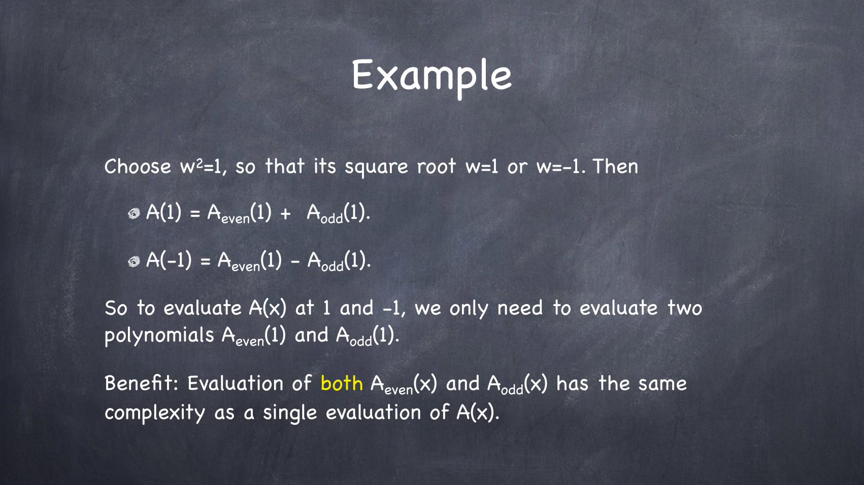
Choose w2=1, so that its square root w=1 or w=-1. Then

A(1) = Aeven(1) + Aodd(1).

A(-1) = Aeven(1) - Aodd(1).

So to evaluate A(x) at 1 and -1, we only need to evaluate two polynomials Aeven(1) and Aodd(1).

Benefit: Evaluation of both Aeven(x) and Aodd(x) has the same complexity as a single evaluation of A(x).

The FFT Trick

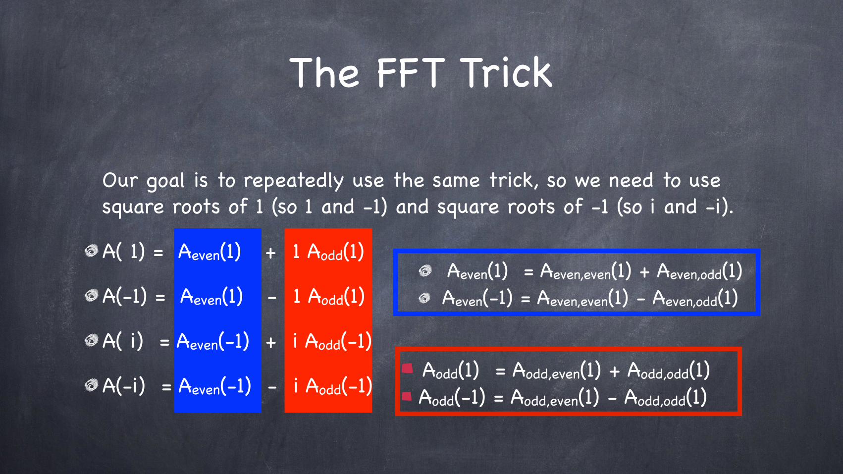
Our goal is to repeatedly use the same trick, so we need to use square roots of 1 (so 1 and -1) and square roots of -1 (so i and -i).

A( 1) = Aeven(1) + 1 Aodd(1)

A(-1) = Aeven(1) - 1 Aodd(1)

A( i) = Aeven(-1) + i Aodd(-1)

A(-i) = Aeven(-1) - i Aodd(-1)

Aeven(1) = Aeven,even(1) + Aeven,odd(1) Aeven(-1) = Aeven,even(1) - Aeven,odd(1)

Aodd(1) = Aodd,even(1) + Aodd,odd(1) Aodd(-1) = Aodd,even(1) - Aodd,odd(1)

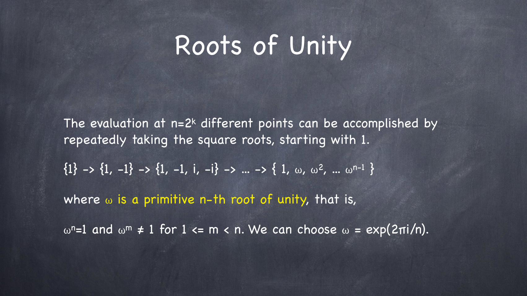
Roots of Unity

The evaluation at n=2k different points can be accomplished by repeatedly taking the square roots, starting with 1.

{1} -> {1, -1} -> {1, -1, i, -i} -> ... -> { 1, ω, ω2, ... ωn-1 }

where ω is a primitive n-th root of unity, that is,

ωn=1 and ωm ≠ 1 for 1 <= m < n. We can choose ω = exp(2πi/n).

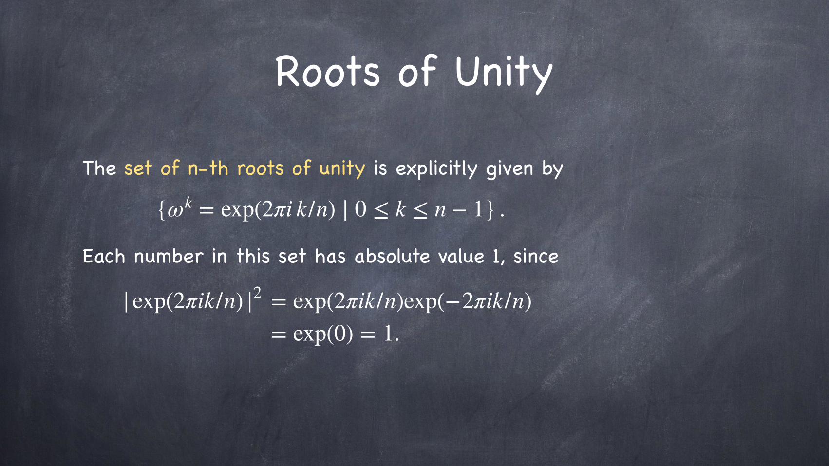
Roots of Unity

The set of n-th roots of unity is explicitly given by

Each number in this set has absolute value 1, since

{ωk = exp(2πi k/n) ∣ 0 ≤ k ≤ n − 1} .

|exp(2πik/n) |2 = exp(2πik/n)exp(−2πik/n)= exp(0) = 1.

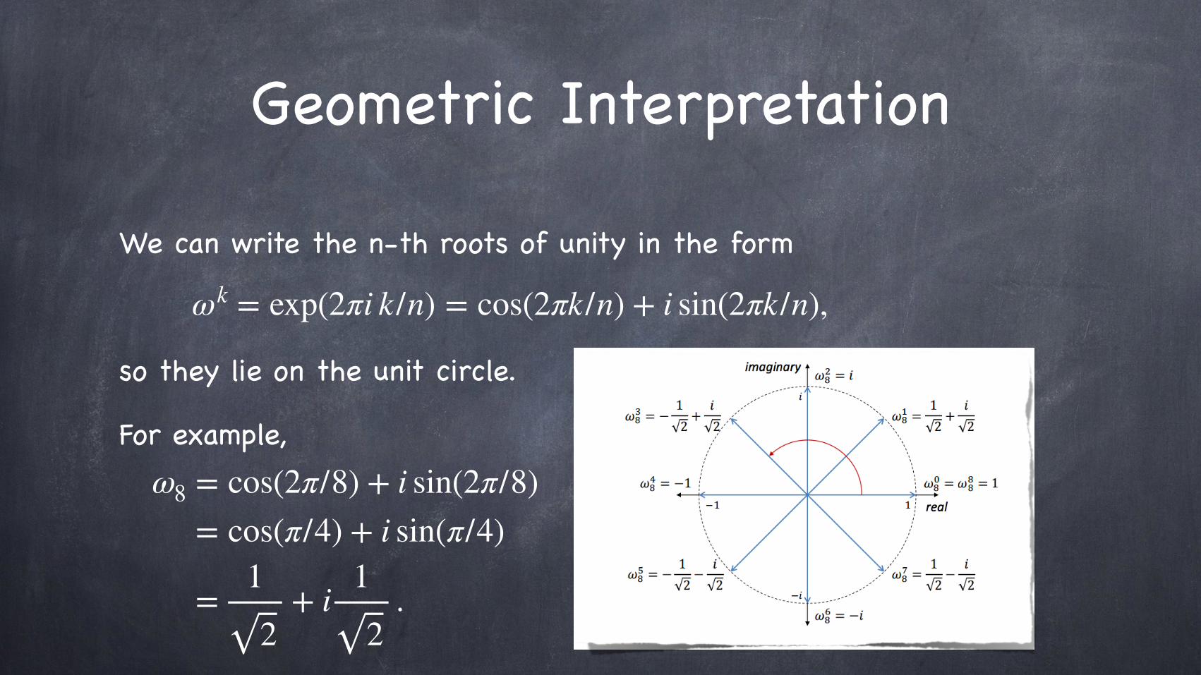
Geometric Interpretation

We can write the n-th roots of unity in the form

so they lie on the unit circle.

For example,

ωk = exp(2πi k/n) = cos(2πk/n) + i sin(2πk/n),

ω8 = cos(2π/8) + i sin(2π/8)= cos(π/4) + i sin(π/4)

=1

2+ i

1

2.

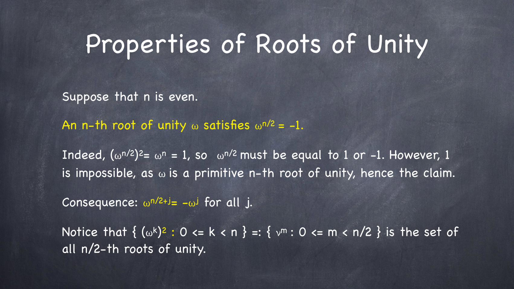
Properties of Roots of Unity

Suppose that n is even.

An n-th root of unity ω satisfies ωn/2 = -1.

Indeed, (ωn/2)2= ωn = 1, so ωn/2 must be equal to 1 or -1. However, 1 is impossible, as ω is a primitive n-th root of unity, hence the claim.

Consequence: ωn/2+j= -ωj for all j.

Notice that { (ωk)2 : 0 <= k < n } =: { νm : 0 <= m < n/2 } is the set of all n/2-th roots of unity.

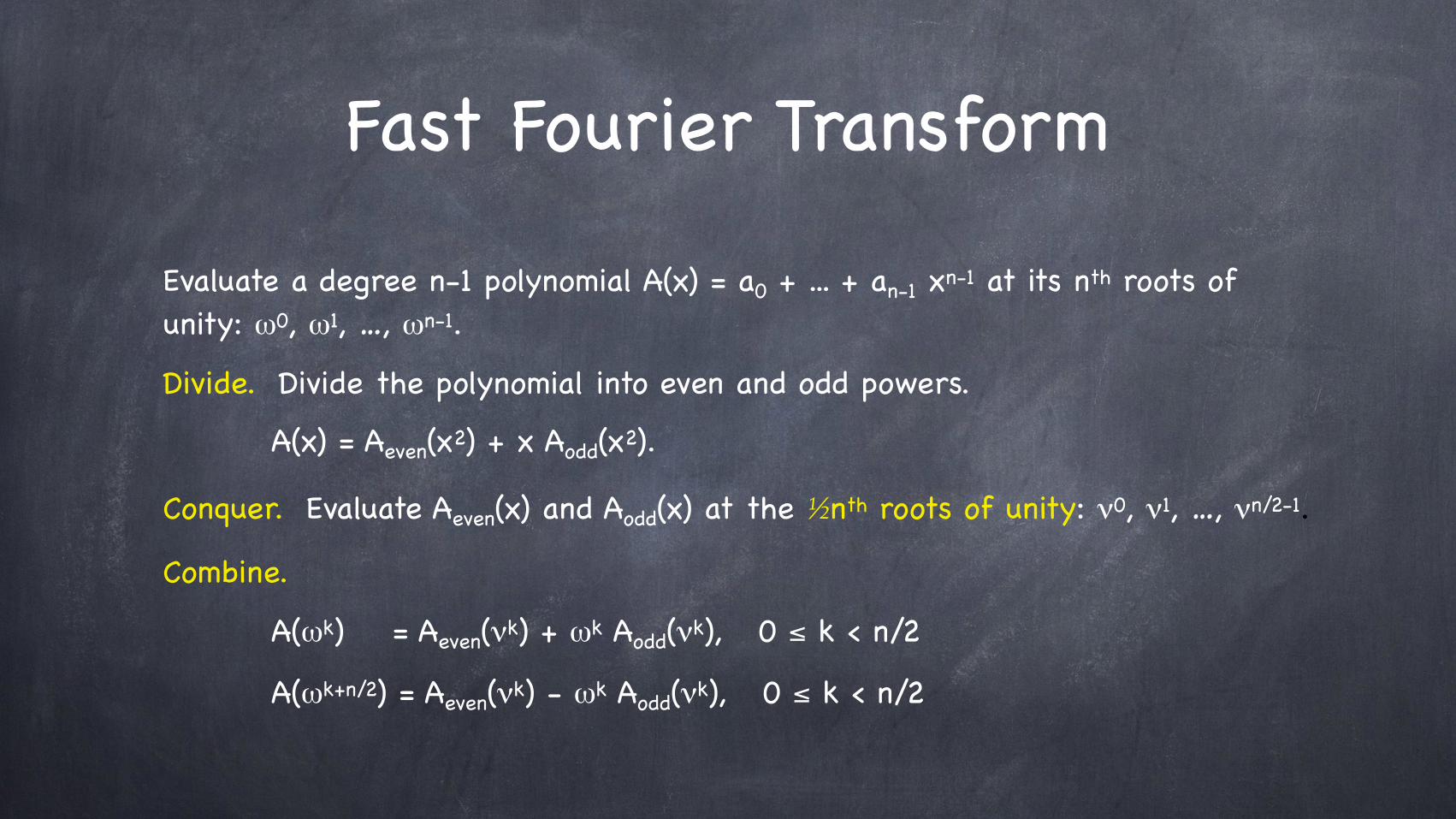
Fast Fourier Transform

Evaluate a degree n-1 polynomial A(x) = a0 + ... + an-1 xn-1 at its nth roots of unity: ω0, ω1, …, ωn-1.

Divide. Divide the polynomial into even and odd powers.

A(x) = Aeven(x2) + x Aodd(x2).

Conquer. Evaluate Aeven(x) and Aodd(x) at the ½nth roots of unity: ν0, ν1, …, νn/2-1.

Combine.

A(ωk) = Aeven(νk) + ωk Aodd(νk), 0 ≤ k < n/2

A(ωk+n/2) = Aeven(νk) - ωk Aodd(νk), 0 ≤ k < n/2

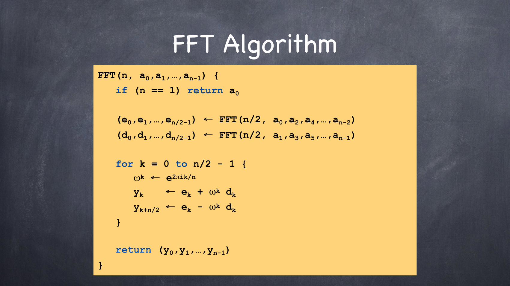
FFT AlgorithmFFT(n, a0,a1,…,an-1) {

if (n == 1) return a0 (e0,e1,…,en/2-1) ← FFT(n/2, a0,a2,a4,…,an-2)

(d0,d1,…,dn/2-1) ← FFT(n/2, a1,a3,a5,…,an-1)

for k = 0 to n/2 - 1 { ωk ← e2πik/n

yk ← ek + ωk dk yk+n/2 ← ek - ωk dk }

return (y0,y1,…,yn-1)

}

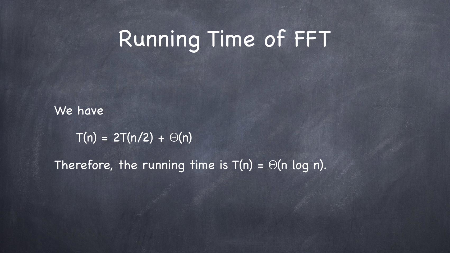
Running Time of FFT

We have

T(n) = 2T(n/2) + Θ(n)

Therefore, the running time is T(n) = Θ(n log n).

Summary

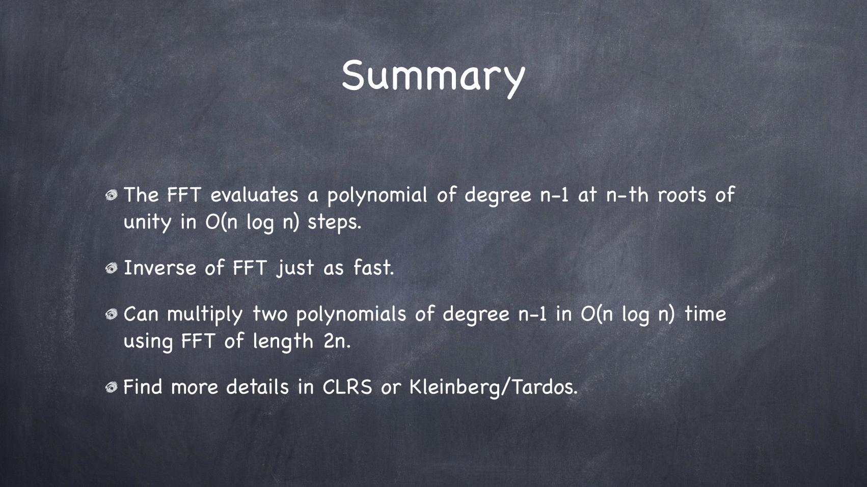
The FFT evaluates a polynomial of degree n-1 at n-th roots of unity in O(n log n) steps.

Inverse of FFT just as fast.

Can multiply two polynomials of degree n-1 in O(n log n) time using FFT of length 2n.

Find more details in CLRS or Kleinberg/Tardos.