arX

iv:a

stro

-ph/

9910

495v

1 2

7 O

ct 1

999

The Extent and Cause of the Pre-White Dwarf Instability Strip

M. S. O’Brien1

Received ; accepted

1Space Telescope Science Institute, 3700 San Martin Drive, Baltimore, MD 21218;

obrien@stsci.edu.

– 2 –

ABSTRACT

One of the least understood aspects of white dwarf evolution is the process

by which they are formed. The initial stages of white dwarf evolution are

characterized by high luminosity, high effective temperature, and high surface

gravity, making it difficult to constrain their properties through traditional

spectroscopic observations. We are aided, however, by the fact that many H-

and He-deficient pre-white dwarfs (PWDs) are multiperiodic g-mode pulsators.

These stars fall into two classes, the variable planetary nebula nuclei (PNNV)

and the “naked” GW Vir stars. Pulsations in PWDs provide a unique

opportunity to probe their interiors, which are otherwise inaccesible to direct

observation. Until now, however, the nature of the pulsation mechanism, the

precise boundaries of the instability strip, and the mass distribution of the

PWDs were complete mysteries. These problems must be addressed before we

can apply knowledge of pulsating PWDs to improve understanding of white

dwarf formation.

This paper lays the groundwork for future theoretical investigations of these

stars. In recent years, Whole Earth Telescope observations led to determination

of mass and luminosity for the majority of the GW Vir pulsators. With these

observations, we identify the common properties and trends PWDs exhibit as a

class.

We find that pulsators of low mass have higher luminosity, suggesting the

range of instability is highly mass-dependent. The observed trend of decreasing

periods with decreasing luminosity matches a decrease in the maximum

(standing-wave) g-mode period across the instability strip. We show that the

red edge can be caused by the lengthening of the driving timescale beyond

the maximum sustainable period. This result is general for ionization-based

– 3 –

driving mechanisms, and it explains the mass-dependence of the red edge. The

observed form of the mass-dependence provides a vital starting point for future

theoretical investigations of the driving mechanism. We also show that the blue

edge probably remains undetected because of selection effects arising from rapid

evolution.

Subject headings: stars: interiors — stars: oscillations — stars: variables:

GW Virginis — white dwarfs

– 4 –

1. Introduction

Until about twenty years ago, the placement of stars in the transition region between

the planetary nebula nucleus track and the upper end of the white dwarf cooling sequence

was problematic. This was due not only to the rapidity with which stars must make this

transition (making observational examples hard to come by) but also to the difficulty of

specifying log g and Teff for such objects. Determining these quantities from spectra requires

that we construct a reasonable model of the star’s atmosphere. This is very difficult for

compact stars with Teff in excess of 50,000 K. The assumption of local thermal equilibrium

(LTE), so useful in modeling the spectra of cooler stars, breaks down severely at such high

temperatures and gravities.

Fortunately, the known sample of stars that occupy this phase of the evolutionary

picture has grown over the last two decades. The most important discovery was that of a

new spectral class called the PG 1159 stars. They are defined by the appearance of lines

of HeII, CIV, and OVI (and sometimes NV) in their spectra. Over two dozen are known,

ranging in Teff from over 170,000 K down to 80,000 K. About half are central stars of

planetary nebula. The most evolved PG 1159 stars merge with the log g and Teff of the

hottest normal white dwarfs. This class thus forms a complete evolutionary sequence from

PNN to the white dwarf cooling track (Werner 1995, Dreizler & Huber 1998).

About half of the PG 1159 stars are pulsating variable stars, spread over the entire

range of log g and Teff occupied by members of the spectral class. This represents the widest

instability “strip” (temperature-wise) in the H-R diagram. Central star variables are usually

denoted as PNNV stars (planetary nebula nucleus variables). Variable PG 1159 stars with

no nebula make up the GW Virginis (or simply GW Vir) stars. PG 1159 thus serves as

the prototype for both a spectroscopic class and a class of variable stars. Farther down the

white dwarf sequence, we find two additional instability strips. At surface temperatures

– 5 –

between about 22,000 and 28,000 K (Beauchamp et al. 1999), we find the DBV (variable

DB) stars. Even cooler are the ZZ Ceti (variable DA) stars, with Teff between 11,300 and

12,500 K (Bergeron et al. 1995). Variability in all three strips results from g-mode pulsation

(for the ZZ Cetis, see Warner & Robinson 1972; for the DBVs, see Winget et al. 1982; for

the PG 1159 variables, see Starrfield et al. 1983). The pulsation periods provide a rich mine

for probing the structure of white dwarf and pre-white dwarf (PWD) stars.

Despite the wealth of pulsational data available to us in studying the variable PWDs,

they have so far resisted coherent generalizations of their group properties. Such a

classification is required for understanding possible driving mechanisms or explaining the

observed period distribution. Until now, the errors bars associated with spectroscopic

determination of mass, luminosity, and Teff for a given variable star spanned a significant

fraction of the instability strip.

Even given the limited information provided by spectroscopic determinations of log g

and Teff , many attempts have been made to form a coherent theory of their pulsations.

Starrfield et al. (1984) proposed that GW Vir and PNNV stars are driven by cyclical

ionization of carbon (C) and oxygen (O). However, their proposal suffers from the difficiency

that a helium (He) mass fraction of only 10% in the driving zone will “poison” C/O

driving. Later, they managed to create models unstable to (C driven) pulsation with

surface He abundance as high as 50%, but only at much lower Teff than most GW Vir stars

(Stanghellini, Cox, & Starrfield 1991; see also the review by Cox, 1993). Another problem

is the existence of non-pulsating stars within the strip with nearly identical spectra to the

pulsators (Werner 1995). More precise observations can detect subtle differences between

the pulsators and non-pulsators. For instance, Dreizler (1998) finds NV in the spectra of all

the pulsators but only some of the non-pulsators. It remains to be seen if these differences

are important.

– 6 –

More recently, Bradley & Dziembowski (1996) studied the effects of using the newer

OPAL opacities in creating unstable stellar models. Their models pulsate via O driving,

and—in exact opposition to Starrfield, Stanghellini, and Cox—they require no C (or He)

in the driving region to obtain unstable modes that match the observed periods. Their

models also require radii up to 30% larger than those derived from prior asteroseismological

analyses of GW Vir stars, in order to match the observed range of periods.

Finally, Saio (1996) and Gautschy (1997) proposed driving by a “metallicity bump,”

where the opacity derivative changes sign due to the presence of metals such as iron in the

envelope. This κ mechanism is similar to those currently thought to drive pulsation in the

β-Cephei variables (see for instance Moskalik & Dziembowski, 1992) and in the recently

discovered subdwarf B variables (Charpinet et al. 1996). Unfortunately, their simplified

models are inconsistent with the evolutionary status of PG 1159 stars. More importantly,

their period structures do not match published WET observations of real pre-white dwarfs

(Winget et al. 1991, Kawaler et al. 1995, Bond et al. 1996, O’Brien et al. 1998).

With so many different explanations for pulsational driving, stricter constraints on

the observable conditions of the pulsators and non-pulsators are badly needed. The most

effective way to thin the ranks of competing theories (and perhaps point the way to

explanations previously unthought of) is to obtain better knowledge of when the pulsations

begin and end for PWD stars of a given mass.

Of course, with only a few stars available to study, even complete asteroseismological

solutions for all of them might not prove significantly illuminating. Even if their properties

follow recognizable patterns, it is difficult to show this compellingly given only a few cases.

However, with asteroseismological analyses now published for the majority of the GW Vir

stars, we can finally attempt to investigate their behavior as a class of related objects. In

the next section, we outline the analytic theory of PWD pulsation. In § 3, we use the

– 7 –

observed properties of the variable PWDs to show that they do follow compelling trends,

spanning their entire range of stellar parameters, to which any model of PWD pulsation

must conform. Next we introduce a new set of numerical models developed to help interpret

this behavior. In § 5, we show how the evolution (and eventual cessation) of pulsation

in PWDs can be governed by the changing relationship of the driving timescale to the

maximum sustainable g-mode period. These results suggest several fruitful directions for

future work, both theoretical and observational, which we discuss in the concluding section.

2. Theory

The set of periods excited to detectable limits in white dwarf stars is determined by

the interplay of several processes. The first is the driving of pulsation by some—as yet

unspecified—mechanism (no matter how melodious the bell, it must be struck to be heard).

Second is the response of the star to the driving taking place somehere in its interior. A

pulsating PWD star is essentially a (spherically symmetric) resonant cavity, capable of

sustained vibration at a characteristic set of frequencies. Those frequencies are determined

by the structure of the star, its mass and luminosity, as well as the thickness of its surface

layers. Finally, the actual periods we see are affected by the mechanism through which

internal motions are translated into observable luminosity variations. This is the so-called

“transfer function,” and clues to its nature are to be found in the observed variations as

well.

2.1. Asyptotic Relations

If we wish to make the most of the observed periods, we must understand the process

of driving, and response to driving, in as much detail as possible. However, we can learn a

– 8 –

great deal by simply comparing the periods of observed light variations to the normal-mode

periods of model stars.

The normal mode oscillations of white dwarf and PWD stars are most compactly

described using the basis set of spherical harmonic functions, Y ℓm, coupled with an

appropriate set of radial wave functions Rn. Here n is the number of nodal surfaces in the

radial direction, ℓ denotes the number of nodal planes orthogonal to such surfaces, and m

is the number of these planes which include the pulsational axis of the star.

The periods of g-modes of a given ℓ are expected to increase monotonically as the

number of radial nodes n increases. The reason is that the buoyant restoring force is

proportional to the total mass displaced, and this mass gets smaller as the number of radial

nodes increases. A weaker restoring force implies a longer period (see, e.g., Cox 1980).

In the “asymptotic limit” that n ≫ ℓ, the periods of consecutive modes should obey the

approximate relation

Πn∼=

Π0

[ℓ(ℓ + 1)]1/2(n + ǫ) n ≫ ℓ, (1)

where Πn is the g-mode period for a given value of n, and Π0 is a constant that depends on

the overall structure of the star (see, e.g., Tassoul 1980, Kawaler 1986).2

Equation (1) implies that modes of a given ℓ should form a sequence based upon a

fundamental period spacing ∆Π = Π0/√

ℓ(ℓ + 1). This is the overall pattern identified by

various investigators in the lightcurves of most of the GW Vir stars. Once a period spacing

is identified, we can compare this spacing to those computed in models to decipher the

star’s structure. Kawaler (1986) found that the parameter Π0 in static PWD models is

2The additional constant ǫ is assumed to be small, though its exact value depends on

the boundary conditions. Since the actual boundary conditions depend on the period, ǫ

probably does, too.

– 9 –

dependent primarily on the overall stellar mass, with a weak dependence on luminosity.

Kawaler & Bradley (1994) present the approximate relation

Π0∼= 15.5

(

M

M⊙

)−1.3 (L

100L⊙

)−0.035 (qy

10−3

)−0.00012

(2)

where qy is the fraction by mass of He at the surface.3

Other questions, however, can only be answered from knowledge of the cause of the

light variations we measure. In the case of the PWDs, this is chief among the mysteries we

would like to solve. The most telling clue will be the extent and location of the region of

instability in the H-R diagram—derived in part from pulsational analysis of the structure

of stars which bracket this region. The will now provide some of the background needed to

attack these issues.

2.2. Pulsation in Pre-White Dwarf Stars

In a star, energy generally flows down the temperature gradient from the central

regions to the surface in a smooth, relatively unimpeded fashion. Of course small, random

perturbations to this smooth flow constantly arise. The situation is stable as long as

such perturbations quickly damp out, restoring equilibrium. For instance, equilibrium is

restored by the forces of buoyancy and pressure; theses forces define the nature of g- and

p-modes. They resist mass motions and local compression or expansion of material away

from equilibrium conditions.

3Note that the sign of the exponent in the L term is in error in Kawaler & Bradley (1994).

– 10 –

2.2.1. Driving and Damping

Thermodynamics and opacity affect local equilibrium. In general, if a parcel of material

in a star is compressed, its temperature goes up while its opacity decreases. The higher

temperature causes more radiation to flow out to the surrounding material, while lower

opacity decreases the efficiency with which radiation is absorbed. From the first law of

thermodynamics, an increasing temperature accompanied by net heat loss implies that work

is being done on the parcel by its surroundings. Similar arguments show that work is done

on the parcel during expansion, also. Thus any initial perturbation will be quickly damped

out—each parcel demands work to do otherwise. The requirement that a region lose heat

when compressing and gain heat when expanding is the fundamental criterion for stability.

When the opposite is true, and work is done by mass elements on their surroundings during

compression and expansion, microscopic perturbations can grow to become the observed

variations in pulsating stars.

Under certain circumstances, the sign of the opacity derivative changes compared to

that described above. If the opacity, κ, increases upon compression, then heat flowing

through a mass element is trapped there more efficiently. Within regions where this is true,

work is done on the surrounding material. Thus, these regions can help destabilize the star,

if this driving is not overcome elsewhere in the star. However, other regions, where work

is required to compress and expand material, tend to damp such pulsation out. Global

instability arises only when the work performed by the driving regions outweighs the work

done on the damping regions over a pulsation cycle. In this case, the flow of thermal energy

can do mechanical work, and this work is converted into the pulsations we observe.

This method of driving pulsation is called the κ mechanism. A region within a star

will drive pulsation via this mechanism if the opacity derivatives satisfy the condition (see

– 11 –

for instance Cox 1980)

d

dr

(

κT +κρ

Γ3 − 1

)

> 0 (3)

where

κT ≡

(

∂lnκ

∂lnT

)

ρ

, κρ ≡

(

∂lnκ

∂lnρ

)

T

, and Γ3 − 1 ≡

(

∂lnT

∂lnρ

)

S

.

Here S represents the specific entropy, κ is the opacity in cm2/g, and the variables r, ρ, and

T all have their usual meaning.

Equation (3) is satisfied most commonly when some species within a star is partially

ionized. In particular, κT usually increases in the hotter (inner) portion of a partial

ionization zone and decreases in the cooler (outer) portion. Thus the inner part of an

ionization zone may drive while the outer part damps pulsation. The adiabatic exponent,

Γ3 − 1, is always positive but usually reaches a minimum when material is partially

ionized. This enhancement of the κ mechanism is called the γ mechanism. Physically, the

γ mechanism represents the conversion of some of the work of compression into further

ionization of the species in question. This tends to compress the parcel more, aiding

the instability. Release of this ionization energy during expansion likewise increases the

purturbation. Since they usually occur together, instabilities caused by both the opacity

and ionization effects are known as the κ-γ mechanism.

The pulsations of Cepheid and RR Lyrae variables, for instance, are driven via the

κ-γ mechanism operating within a region where HeI and HeII have similar abundances.

This same partial ionization zone is apparently the source of instability for the DBV white

dwarfs. The variations observed in ZZ Ceti white dwarfs have long been attributed to partial

ionization of H. However, Goldreich & Wu (1999a,b,c) have recently shown the ZZ Ceti

pulsations can be driven through a different mechanism in efficient surface convection.4

Great efforts have been expended by theorists attempting to explain GW Vir and PNNV

4Such convection zones often accompany regions of partial ionization associated with the

– 12 –

pulsations in terms of some combination of C and O partial ionization (Starrfield et al. 1983;

Stanghellini, Cox, & Starrfield 1989; Bradley & Dziembowski 1996). A primary difficulty

arises from the damping effects of He (and C in the O-driving scheme proposed by Bradley

& Dziembowski 1996) in the driving zone, which can “poison” the driving. More recently,

Saio (1996) and Gautschy (1997) attempted to explain driving in terms of an “opacity

bump” in the models, without partial ionization—in other words, using the κ mechanism

alone. A fundamental problem has been the lack of information on the exact extent of the

instability strip and the structure of the pulsating stars themselves. The initial goal in this

paper, therefore, is to define as precisely as possible the observational attributes which any

proposed driving source must reproduce. Whether or not the mechanism we later identify

is correct, we hope to lay the groundwork for future studies which will eventually provide a

definitive answer to this question.

If a star pulsates, we wish to know what relationship the driving has to the periods

we observe. In general, no star will respond to driving at just any arbitrary period; the

pulsation period range is determined by the driving mechanism. Cox (1980) showed that

the approximate pulsation period is determined by the thermal timescale of the driving

zone:

Π ∼ τth =cvTmdz

L. (4)

Here τth is the thermal timescale, cv is the heat capacity, and mdz is the mass above

the driving zone. This equation gives the approximate time it takes the star to radiate

away—via its normal luminosty, L—the energy contained in the layers above the region in

κ-γ mechanism. However, the driving proposed by Goldreich & Wu is not directly related

to ionization. It is possible this theory might eventually be expanded to account for DBV

pulsation as well. It is unlikely to find application in PWDs, though, since models of PG 1159

stars generally do not support convection.

– 13 –

question. Though Cox derived this relationship for radial modes, Winget (1981) showed

that it applies equally well to nonradial g-mode pulsation.

The basic idea behind Equation (4) is that energy must be modulated at approximately

the same rate at which it can be dammed up and released by the driving zone. Consider the

question of whether a given zone can drive pulsation near a certain period. If the driving

zone is too shallow, then the thermal timescale is shorter than the pulsation period. Any

excess heat is radiated away before the compression increases significantly. Thus, it can’t

do work to create mechanical oscillations on the timescale in question. If the driving zone

is too deep (τth > Π), then excess heat built up during contraction is not radiated away

quickly enough during expansion; it then works against the next contraction cycle. Of

course, this relationship is only approximate, and other factors might intervene to limit

pulsation to periods far from from those implied by Equation (4).

2.2.2. Period Limits

One such factor is the range of pulsation modes a star can sustain in the form of

standing waves. Hansen, Winget, & Kawaler (1985) showed that there is a maximum period

for white dwarf and PWD stars above which oscillations will propagate only as running

waves that quickly damp out. They attempt to calculate this maximum g-mode period,

Πmax, to explain the observed trend of ZZ Ceti periods with Teff . We can recast their

equations (6) through (8) as

Πmax ≈ 940s

(

µ

ℓ(ℓ + 1)

)0.5 (R

0.02R⊙

)

(

Teff

105K

)−0.5

, (5)

or, using the relation R2 = L/4πσT 4eff ,

Πmax ≈ 940s

(

µ

ℓ(ℓ + 1)

)0.5 (L

35L⊙

)0.5 (Teff

105K

)−2.5

. (6)

– 14 –

where R is the stellar radius, µ represents the mean molecular weight, and ℓ is the pulsation

index introduced earlier. For a complete derivation of these equations, see the Appendix.

For cool white dwarfs of a given mass, the radius is roughly constant with time, and

Πmax is expected to increase as stars evolve to lower Teff and the driving zone sinks deeper.

Cooler ZZ Ceti and DBV white dwarf stars should in general have longer periods; for the

ZZ Cetis at least, this is indeed the case.

However, in PWDs degeneracy is not yet sufficient to have halted contraction, and the

R dependence is still a factor in determining how Πmax varies through the instability strip.

We cannot say a priori which dominates: the shrinking radius which tends to decrease

Πmax, or the falling Teff which has the opposite effect. We cannot even predict in advance

whether Πmax is a factor in determining the pulsation periods at all. In § 5, we answer these

questions in view of the observed properties of both the PNNV and GW Vir stars.

In summary, we can measure individual white dwarf mass and luminosity through

identification of the period spacing. The resulting determinations of GW Vir structure,

summarized in the next section, will tell us the precise boundaries of the instability strip,

in other words, when the pulsations begin and end in the evolution of PWD stars of a

given mass. This knowledge, coupled with the timescales of driving and the maximum

g-mode period in models matched to the observations, will provide strict constraints on the

allowable form of the driving mechanism. This information is absolutely necessary to any

research program designed to discover why PWDs pulsate in the first place.

3. Observed Temperature Trends of the PG 1159 Pulsators

– 15 –

3.1. Mass Distribution

White dwarfs exhibit a very narrow mass distribution, centered at about 0.56–0.59 M⊙

(Bergeron, Saffer & Liebert 1992, Weidemann & Koester 1984). If, for a given Teff ,

pulsating PWD masses conform to the same distribution expected of non-variables, then

we are led to certain expectations concerning the pulsations seen in the former. Based on

Equations (1) and (2), period spacing (proportional to Π0) should increase monotonically

as the luminosity and Teff of a given star decrease.

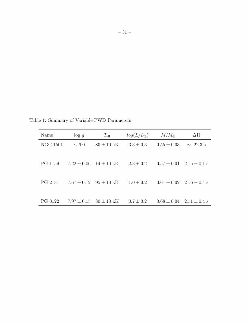
Four PWD stars have so far yielded to asteroseismological scrutiny, the GW Vir stars

PG 1159 (Winget et al. 1991), PG 2131 (Kawaler et al. 1995), and PG 0122 (O’Brien et

al. 1998), and the central star of the planetary nebula NGC 1501 (Bond et al. 1996). We

summarize the parameters of these four stars in Table 1. All show patterns of equal period

spacing very close to 21 s. This is a remarkable trend, or more accurately, a remarkable

lack of a trend! If these stars follow the narrow mass distribution observed in white dwarf

stars, then the period spacing is expected to increase with decreasing Teff as they evolve

from the blue to the red edge of the instability strip. Observationally, this is not the case.

For instance PG 1159, with a Teff of 140,000 K, should see its period spacing increase

by about 20%, from 21 s to 26 s, by the time it reaches the effective temperature of

PG 0122—80,000 K. In other words, the farther PG 0122’s period spacing is from 26 s,

the farther is its mass from that of PG 1159. In fact these two objects, representing the

high and low Teff extremes of the GW Vir stars, have almost exactly the same period

spacing despite enormous differences in luminosity and temperature. For PG 0122, its

low Teff pushes it toward longer ∆Π; this must be offset by a higher mass. With such

a significant Teff difference, the mass difference between PG 0122 and PG 1159 must be

significant also, and it is: 0.69 M⊙ versus 0.58 M⊙.

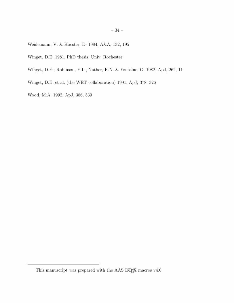
Two stars with a coincident period spacing—despite widely different mass and

– 16 –

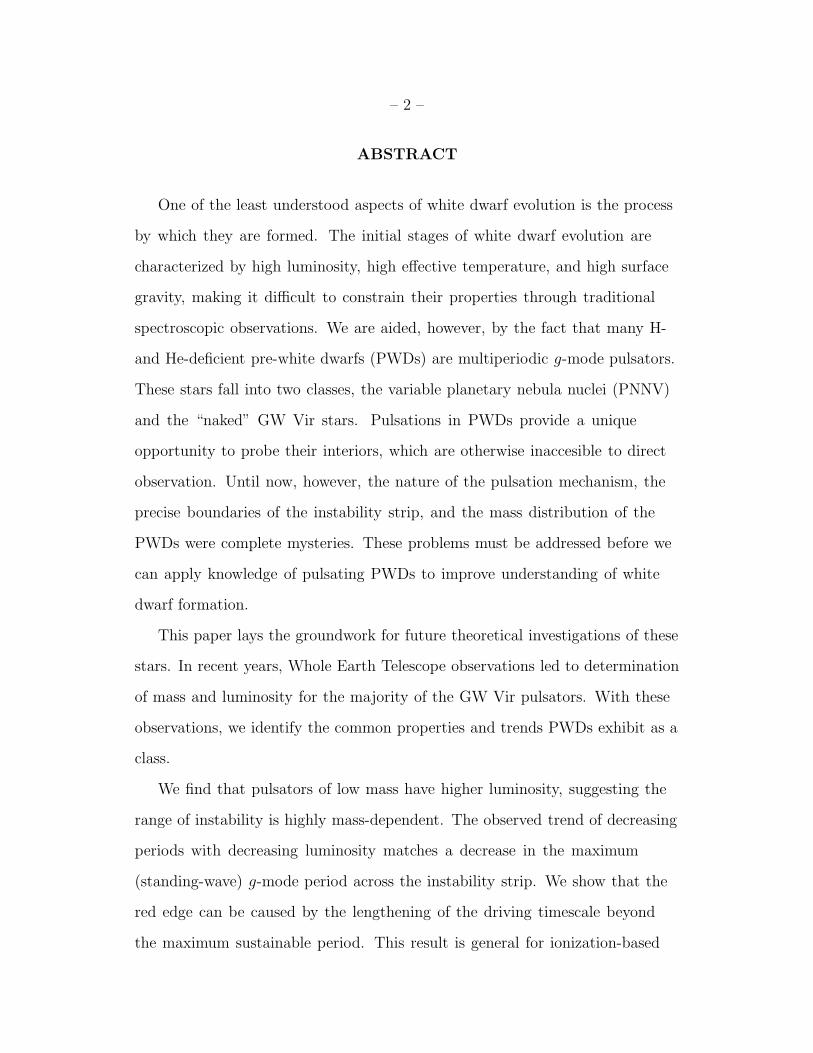
luminosity—might simply be curious. In fact all four PWDs with relatively certain period

spacing determinations have the same spacing to within 2 s, or 10%. This includes the

central star of NGC 1501, which has a luminosity over three orders of magnitude larger

than that of PG 0122. Hence, NGC 1501 must have an even lower mass than PG 1159 by

comparison. Figure 1 shows the mass versus luminosity values for the known GW Vir stars

plus NGC 1501, based on the values of ∆Π from Table 1.

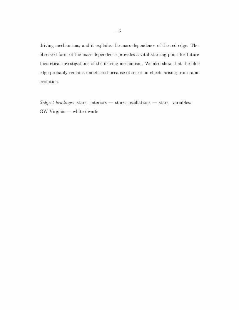
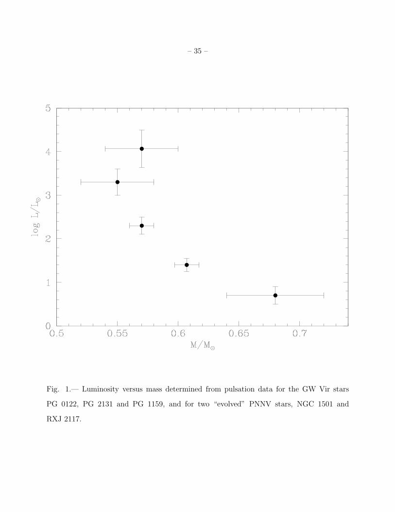
Figure 2 shows the implications of the common 21-22 s spacing for the instability

“strip” in the log g–log Teff plane. The observational region of instability has shrunk

significantly. It exhibits such a striking slope in the figure that, unlike most other instability

regions in the H-R diagram, it can no longer be refered to accurately as an instability strip

(in temperature) at all. Nevertheless, we will continue to refer to the region of instability

pictured in Figure 2 as the GW Vir “instability strip” with the understanding that the

effective temperatures of the red and blue edges are highly dependent on log g (or L).

Why should the PWD instability strip apparently straddle a line of approximately

constant period spacing? Normally, theorists search for explanations for the observed

boundaries (the red and blue edges) of an instability strip based on the behavior of a

proposed pulsation mechanism. That behavior is determined by the thermal properties of a

PWD star, while its period spacing is determined by its mechanical structure. In degenerate

or nearly degenerate stars, the thermal properties are determined by the ions, while the

mechanical structure is determined by the degenerate electrons, and normally the two are

safely treated as separate, isolated systems. If the 21-22 s period spacing is somehow a

prerequisite for pulsation, then this implies an intimate connection between the mechanical

oscillations and the thermal pulsation mechanism.

The alternative is that the mass-luminosity relationship along the instability strip is

caused by some other process—or combination of processes—which approximately coincides

– 17 –

with the relationship that governs the period spacing. In this case, some mechanism must

shut off observable pulsation in low mass PWDs before they reach low temperature, and

delay observable pulsation in higher mass PWDs until they reach low temperature.5 We

will explore mechanisms which meet these criteria in § 5.

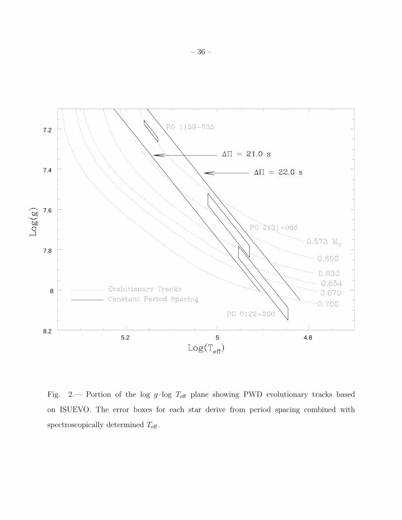
3.2. Period Distribution

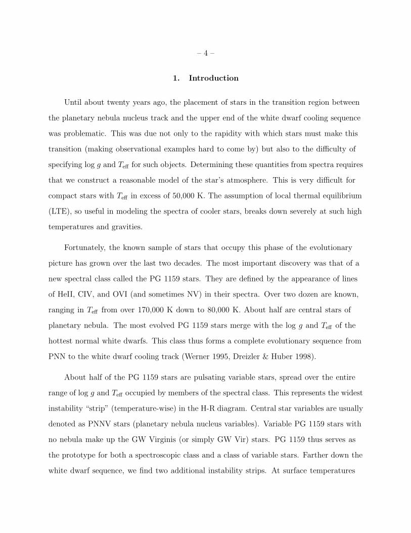
The PWD pulsators exhibit another clear observational trend: their periods decrease

with decreasing luminosity (increasing surface gravity). Figure 3 shows the luminosity

versus dominant period (that is, the period of the largest amplitude mode) for the same

stars from Figure 1. The trend apparent in the figure is in marked contrast to the one seen

in the ZZ Ceti stars, which show longer periods with lower Teff . The ZZ Ceti period trend

is generally attributed to the changing thermal timescale in the driving zone, which sinks

deeper (to longer timescales) as the star cools. If the same effect determines the periods

in GW Vir and PNNV stars, then Figure 3 might be taken to indicate that the driving

zone becomes more shallow with decreasing Teff . We will show that this is not the case in

PWD models. We conclude that some other mechanism must be responsible for setting the

dominant period in PWD variables.

Are the trends seen in Figures 1 through 3 related? To explore this question in detail,

we developed a new set of PWD evolutionary models, which we summarize in the next

section. In § 5 we analyze the behavior of driving zones in PWD models in light of—and to

seek an explanation for—the trends just discussed.

5We use the phrase “observable pulsation” to indicate that possible solutions might reside

in some combination of observational selection effects as well the intrinsic behavior of a

driving mechanism.

– 18 –

4. A New Set of Pre-White Dwarf Evolutionary Models

To understand the various trends uncovered in the hot pulsating PWDs, we appeal

to stellar models. Models have been essential for exploiting the seismological observation

of individual stars. For this work, though, we needed models over the entire range of the

GW Vir stellar parameters of mass and luminosity. Our principal computational tool is

the stellar evolution program ISUEVO, which is described in some detail by Dehner (1996;

see also Dehner & Kawaler 1995). ISUEVO is a “standard” stellar evolution code that is

optimized for the construction of models of PWDs and white dwarfs.

The seed model for the models used in this section was generated with ISUEVO

by evolution of a 3 M⊙ model from the Zero Age Main Sequence through the thermally

pulsing AGB phase. After reaching a stable thermally pulsing stage (about 15 thermal

pulses), mass loss was invoked until the model evolved to high temperatures. This model

(representing a PNN) had a final mass of 0.573 M⊙, and a helium-rich outer layer.

To obtain self-consistent models within a small range of masses, we used the 0.573 M⊙

model, and scaled the mass up or down. For example, to obtain a model at 0.60 M⊙,

we scaled all parameters by the factor 0.60/0.573 for an initial model. Relaxation to the

new conditions was accomplished by taking many very short time steps with ISUEVO.

Following this relaxation, the evolution of the new model proceeded as before. In this way,

we produced models that were as similar as possible, with mass being the only difference.

Comparison of our evolutionary tracks and trends with the earlier model grids of Dehner

(1996) shows very close agreement, given the different evolutionary histories. Dehner’s

initial models were derived from a single model with a simplified initial composition profile,

while our models are rooted in a self-consistent evolutionary sequence. We note that the

work by Dehner (1996) included elemental diffusion (principally by gravitational settling),

while the models we use here did not include diffusion. Within the temparature range of the

– 19 –

GW Vir stars, however, observations of their surface abundances indicate that the effects of

diffusion have only a small influence.

5. Selection Effects, Driving, and the Blue and Red Edges

5.1. The Observed “Blue” and “Red” Edges

In explaining the observed distribution of pulsating stars with respect to stellar

parameters, we must distinguish observational selection effects from causes intrinsic to

the objects under study. Usually, understanding selection effects is an important part of

decoding the shape of the distribution in terms of physical effects. In this case, the blue

and red edges exhibit a similar slope in the log g–log Teff plane, but we must still separate

out selection effects from the intrinsic shape of one or both of them.

The more rapid the evolution through a particular region of the H-R diagram, the less

likely it is that stars will be found there. Also, the relative sample volume is larger for stars

with higher luminosity, since they are detectable at greater distances. Some combination of

these effects will determine the odds of finding stars of a particular mass at a particular

point in their evolution. One of the most common ways to explore these combined effects is

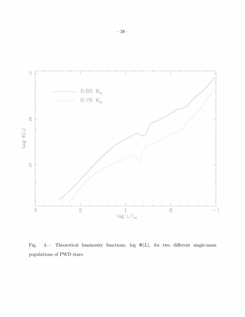
to construct a luminosity function, which is simply a plot of the expected number density

of stars per unit luminosity, based on how bright they are and how fast they are evolving

at different times. Figure 4 shows schematic luminosity functions for PWD stars of two

different masses, based on the models described in the previous section and normalized

according to the white dwarf mass distribution (see for instance Wood 1992). One important

result of this figure is that higher mass models always achieve a given number density

per unit luminosity later (at lower L and Teff) than lower mass models. Also, the number

density per unit luminosity increases for all models as they evolve to lower Teff , due to the

– 20 –

increasing amount of time spent in a luminosity bin.

These effects together imply that, if PWDs of all mass pulsate all the way down to

80,000 K, then the distribution of known pulsators should be skewed heavily toward those

with both low Teff and low mass. We don’t see such stars; thus the red edge must exclude

the low mass, low Teff stars from the distribution.

While the observed red edge actually marks the dissappearance of pulsations from

PWD stars, selection effects change our chances of finding high-mass, high-Teff pulsators.

In this case, we expect that the likehood of finding stars of a given mass within the

instability strip will increase the closer those stars get to the red edge. This would tend

to render the theoretical blue edge (as defined by the onset of pulsation in models of a

given mass) undetectible in real PWD stars—given the small number of known variables.

In other words, stars “bunch up” against the red edge due to their continually slowing rate

of evolution, causing the apparent blue edge to shadow the slope of the red edge in the

log g–log Teff plane. This could explain the approximately linear locus of pulsating stars

found within that plane implied by their tight distribution of ∆Π.

We are left to explain the observed red edge in terms of the intrinsic properties of the

stars themselves, which we defer to § 5.3. First, however, we will discuss the effects of the

observed mass distribution along the strip on the period trend seen in Figure 3.

5.2. The Π versus Teff Trend

As mentioned previously (and as we show in § 5.3, below), the depth of an ionization-

based driving zone increases—moves to larger thermal timescales—with decreasing Teff for

PWD stars of a given mass. This implies a period trend opposite to that observed in

Figure 3. Bradley & Dziembowski (1996) discuss this very problem, since their models

– 21 –

predict that the maximum period of unstable modes should increase as Teff decreases. They

suggest that the composition of the driving zone might somehow change with time, or that

the stellar radii shrink much more quickly than is currently thought (or some combination of

the two), in such a way as to make the maximum unstable period decrease with decreasing

Teff . However, no one has yet calculated how (and whether) these suggestions could

reasonably account for the observed trend. It is clear, however, that something other than

the depth of the driving zone alone determines the observed period range.

What other mechanisms might affect the observed periods? One such mechanism is the

changing value of the maximum sustainable g-mode period, Πmax. For the ZZ Ceti stars,

Πmax probably does not influence the period distribution much, since from Equations (5)

and (6) it increases through the ZZ Ceti instability strip. In PWDs, however, the R

dependence in Equation (5) must be taken into account; we cannot be certain that the

trend implied by a lengthening driving timescale won’t find itself at odds with a decreasing

Πmax.

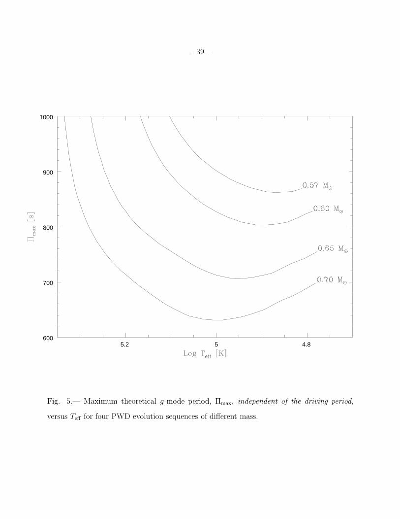
Figure 5 shows the (arbitrarily normalized) run of Πmax versus Teff for three PWD

model sequences of different mass. Clearly, Πmax decreases significantly as models evolve

along all three sequences, with high-mass stars exhibiting a smaller Πmax than low-mass

stars at all Teff .6 These two effects, when combined with the PWD mass distribution,

imply that Πmax should plummet precipitously with increasing log g in the models shown

in Figure 2. For example, the ratio of Πmax for PG 1159 to that of PG 0122 is expected to

be ∼ 1.42:1, while the ratio of their observed dominant periods is 540:400 = 1.35:1. The

6If this trend continued all the way to the cooler white dwarf instability strips, then

ZZ Ceti stars could only pulsate at very short periods, but Teff begins to dominate below

around 60,000 to 70,000 K, pushing Πmax back to longer and longer periods once the stars

approach their minimum radius at the top of the white dwarf cooling track.

– 22 –

period distribution seen in Figure 2 is thus consistent with the idea that the value of Πmax

determines the dominant period in GW Vir stars. As we will see in the next section, Πmax

probably also plays an important part in determining the more fundamental question of

when a given star is likely to pulsate.

5.3. Driving Zone Depth, Πmax, and the Red Edge

In § 2.2, we discussed the relationship between the depth of the driving zone and

the period of g-mode oscillations. Equation (4) implies that the dominant period should

increase in response to the deepening driving zone, as long as other amplitude limiting

effects do not intervene. Figure 5 shows how one particular effect—the decreasing maximum

period—might reverse the trend connected to driving zone depth, and the observed periods

of GW Vir stars supports the suggestion that Πmax is the key factor in setting the dominant

period. While Πmax limits the range of periods that can respond to driving, τth in the

driving zone limits the periods that can be driven. However, τth increases steadily for all

GW Vir stars, and Πmax decreases steadily. Eventually, therefore, every pulsator will reach

a state where τth > Πmax over the entire extent of the driving zone. In such a state, the star

can no longer respond to driving at all, and pulsation will cease. If Πmax remains the most

important amplitude limiting factor for stars approaching the red edge, then the red edge

itself could be caused by the situation just described.

We can test this idea by asking if it leads to the kind of mass-dependent red edge

we see. To answer this question, we need to know how the depth of the driving zone (as

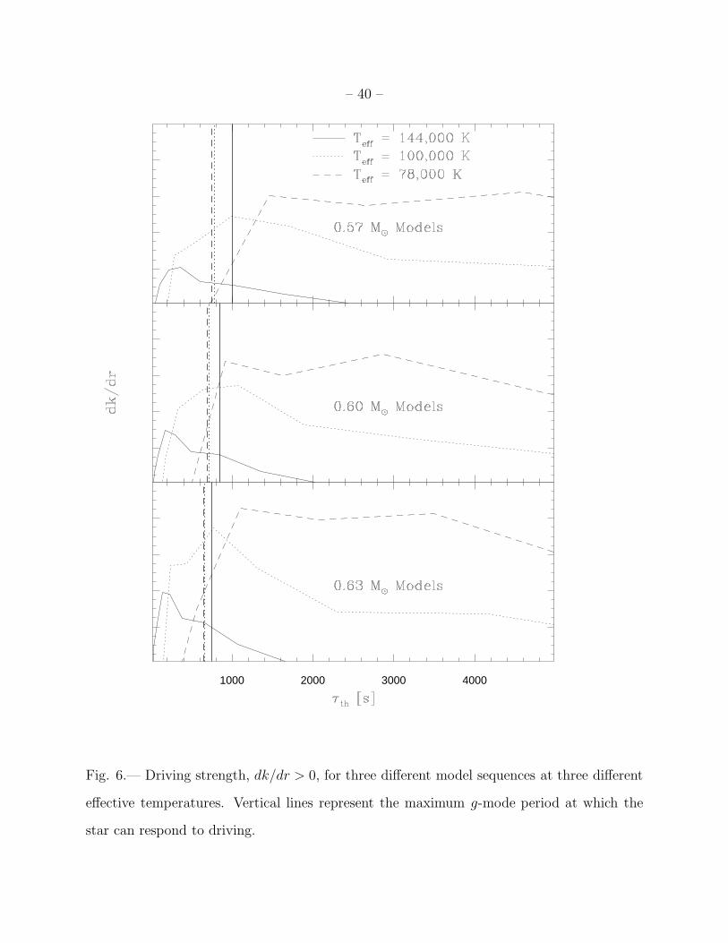
measured by τth) changes with respect to Πmax for stars of various mass. Figure 6 depicts

the driving regions for three different model sequences (M = 0.57, 0.60 and 0.63 M⊙) at

three different effective temperatures (144,000 K, 100,000 K, and 78,000 K). The driving

strength, dk/dr, is determined from Equation (3), where k represents the expression inside

– 23 –

parentheses. The vertical axis has not been normalized and is the same scale in all three

panels. The surface of each model is on the left, at τth = 0. The vertical lines in the

figure represent Πmax, for each model, normalized to 1000 s in the 0.57 M⊙ model at

144,000 K. We have made no attempt to calculate the actual value of Πmax (however, see

the Appendix); the important thing is its changing relationship to the depth of the driving

zone with changing mass and Teff .

A couple of important trends are clear in the figure. First, the driving zone in models

of a given mass sinks to longer τth, and gets larger and stronger, with decreasing Teff . In

the absence of other effects, this trend would lead to ever increasing periods of larger and

larger amplitude as Teff decreases. Meanwhile, Πmax changes more moderately, moving

toward slightly shorter timescales with decreasing Teff and increasing mass. If we make

the somewhat crude assumption that the effective driving zone consists only of those parts

of the full driving zone with τth < Πmax, then a picture of the red edge emerges. At

Teff =144,000 K, the driving zone is relatively unaffected in all three model sequences. As

Teff decreases, and the driving zone sinks to longer τth, the Πmax-imposed limit encroaches

on the driving zone more and more for every mass. Thus the longer periods, while driven,

are eliminated, moving the locus of power to shorter periods than would be seen if Πmax

was not a factor. Eventually, all the driven periods are longer than the maximum period at

which a star can respond, and pulsation ceases altogether. This is the red edge.

Pulsations will not shut down at the same Teff in stars of every mass. High mass

models retain more of their effective driving zones than low mass models at a given Teff .

This occurs because at a given Teff , the top of the driving zone moves toward the surface (to

smaller τth) with increasing mass. This effect of decreasing τth at the top of the driving zone

outstrips the trend to lower Πmax with increasing mass. The result is that, at 78,000 K,

the driving zone in the 0.57 M⊙ model (upper panel of Figure 6) has moved to timescales

– 24 –

entirely above the Πmax limit, while the 0.63 M⊙ model (appropriate for PG 0122: see the

bottom panel in Figure 6) still produces significant driving at thermal timescales below

Πmax.

Recall from Table 1 and Figure 2 that GW Vir stars of lower Teff have higher mass.

Why? We can now give an answer: at low Teff , the low mass stars have stopped pulsating

because they only drive periods longer than those at which they can respond to pulsation!

Higher mass stars have shallower ionization zones (at a given Teff) that still drive periods

shorter than the maximum allowed g-mode period, even at low Teff . This causes the red

edge to move to higher mass with decreasing luminosity and Teff , the same trend followed

by lines of constant period spacing. The interplay between driving zone depth and Πmax

enforces the strikingly small range of period spacings (∆Π ∼ 21.5 s) seen in Table 1 and

Figure 2.

These calculations are not an attempt to predict the exact location of the red edge at

a given mass. We are only interested at this point in demonstrating how the position of

the red edge is expected to vary with mass, given an ionization-based driving zone with

an upper limit placed on it by Πmax. In the particular models shown in Figure 6, the top

of the driving zone corresponds to the ionization temperature of OVI, but the behavior of

the red edge should be the same no matter what species causes the driving. Its absolute

location, though, would probably be different given driving by different species. In order

to use the location of the red edge for stars of different mass to identify the exact species

that accomplishes driving, we would need to calculate Πmax precisely for all the models in

Figure 6 and better understand exactly how the value of Πmax affects the amplitudes of

modes nearby in period. Such a calculation is beyond the scope of this paper, and we leave

it to future investigations to attempt one.

Alternatively, the discovery of more GW Vir stars would help us better understand

– 25 –

these processes by defining the red edge with greater observational precision. The simplest

test of our theories would be to find low-Teff GW Vir pulsators of low mass. If they exist,

then Πmax is probably not a factor in determining their periods, and variation should be

sought in their lightcurves at longer periods than in the GW Vir stars found so far; Figure 6

suggests their dominant periods should be in the thousands of seconds. It is possible that

these stars could be quite numerous (and should be quite numerous if they exist at all, given

their slower rate of evolution) and still escape detection, since standard time-series aperture

photometry is not generally effective at these timescales. Most current CCD photometers

are quite capable of searching for such variability, however. Based on these results, we

encourage future studies to determine whether or not low-mass, low-Teff GW Vir pulsators

do indeed exist.

6. Summary and Conclusions

Our purpose is to understand how and why PWD stars pulsate, so that astronomers

can confidently apply knowledge of PWD structure—gained via asteroseismology—to study

how white dwarfs form and evolve and better understand the physics that governs these

processes. We have pursued PWD structure via the pulsation periods and the additional

constraints they provide for our models. A surprising similarity emerged among them:

their patterns of average period spacing span a very small range from 21–23 s. Including

the PNNV star NGC 1501, this uniformity extends over three orders of magnitude in PWD

luminosity. Since the average period spacing increases with decreasing luminosity—and

decreases with increasing mass—this result implies a trend toward significantly higher mass

with decreasing luminosity through the instability strip. This trend has several important

implications for our understanding of PWD pulsations.

The instability is severely sloped toward lower Teff with stellar mass increasing down the

– 26 –

instability strip. To understand this sloped instability strip, we needed information inherent

in the other fundamental observed trend: the dominant period in PWD pulsators decreases

with decreasing luminosity. We found that the observed dominant period is correlated

with the theoretical maximum g-mode period, Πmax. If Πmax is a factor in determining the

range of periods observed in pulsating PWD stars, then it should play a role in determining

when pulsation ceases, because the driving zone tends to drive longer and longer periods

in models of given mass as the models evolve to lower Teff . At low enough temperatures,

the driving zone is only capable of driving periods longer than Πmax, and pulsations should

then cease. Since the top of the driving zone moves to shorter timescales with increasing

mass, and does so faster than Πmax decreases with increasing mass, higher mass models

should pulsate at lower Teff than lower mass models. This behavior is compatible with the

observed slope of the red edge in the log g–log Teff plane.

This mechanism does not account for the lack of observed high-mass pulsators at

high Teff , however. Theoretical luminosity functions for the PWD stars indicate the observed

blue edge is probably significantly affected by selection effects due to rapid evolution at high

Teff . Since higher mass models are both less numerous and less luminous at a given Teff than

models of lower mass, we are more likely to detect low-mass than high-mass PWDs at a

given temperature. This will cause stars to “bunch up” against the red edge in the observed

instability strip, and the apparent blue edge will thus “artificially” resemble the shape of

the red edge—no matter what the true shape might be. This selection effect, in isolation,

would imply that low-mass, low Teff GW Vir pulsators should be most numerous of all.

That we in fact find none strengthens our contention that the mass-dependence of the red

edge is a real effect—we find no low-mass, low-Teff GW Vir stars because they don’t exist.

The boundaries of the PWD instability strip derived from our pulsation studies are

far smaller than those based on spectroscopic measurements alone. Though the actual

– 27 –

range of log g and Teff spanned by the known pulsators is no smaller than before, the newly

discovered mass-luminosity relationship implies that the width of the strip in Teff at a given

log g is quite small, and vice versa. We can therefore no longer say for certain that any

non-pulsators occupy this newly diminished instability strip, since the uncertainties in log g

and Teff as determined from spectroscopy are larger now than the observed width of the

strip itself at a given log g or Teff .

This highlights the importance of finding additional pulsators with which to further

refine our knowledge of the instability strip boundaries. In particular, we still have no

observations with which to constrain theories of the blue edge, since there is no reason that

the instrinsic blue edge lies near the observed blue edge at any effective temperature.

If the trend we have discovered continues down to effective temperatures below the

coolest known pulsating PWDs, then high-mass (∼ 1 M⊙ or greater) white dwarfs might

pulsate at temperatures as low as 50,000–60,000 K (and log g ∼ 8). Their dominant periods

(again, assuming they follow the trends outlined in § 3 and § 5) would be shorter than

any known PWDs, perhaps as low as 200-300 s. Such stars would not be PWDs at all but

rather white dwarfs proper. Their discovery would complete a “chain” of variable stars

from PNN stars to “naked” PWDs to hot white dwarfs, and as such they would represent a

incalculable boon to astronomers who study the late stages of stellar evolution.

On the theory side, we need to understand how PWD stars react to driving near the

maximum g-mode period. Studies should be undertaken to determine the actual maximum

period in PWD models. PWD evolution sequences should be constructed that contain all

the elements thought to exist in PWD stars. We have observational information to test all

these calculations, and with the observational program proposed above, we will gain more.

There is much to do.

– 28 –

The author expresses deepest gratitude to Steve Kawaler and Chris Clemens, who

together taught him the crafts of astronomy: theory, observation, and communication.

Their sage council and unblinking criticism greatly enhanced the quality of this work.

I am also indebted to Paul Bradley, whose thoughtful insights substantially improved

both the content and presentation of this paper.

A. The Maximum Period

A variable pre-white dwarf star is a resonant cavity for non-radial g-mode oscillations.

This spherically symmetric cavity is bounded by the stellar center (or the outer edge

of the degenerate core in ZZ Ceti and DBV white dwarfs) and surface. At sufficiently

long periods, however, the surface layers no longer reflect internal waves. The pulsation

energy then leaks out through the surface, damping the pulsation. This idea was first

applied to white dwarf pulsations by Hansen, Winget & Kawaler (1985), who attempted to

calculate the approximate critical frequencies to explain both the red edge and maximum

observed periods in ZZ Ceti stars. Assuming an Eddington gray atmosphere, they derive

the following expression for the dimensionless critical g-mode frequency:

ω2

g ≈ℓ(ℓ + 1)

Vg(A1)

where

Vg =3gµR

5NakTeff

. (A2)

Here g and R represent the photospheric surface gravity and radius, and Na, k, and µ have

their usual meaning.

The dimensionless frequency, ω, is related to the pulsation frequency, σ, according to

ω2 =σ2R

g. (A3)

– 29 –

The pulsation period is Π = 2π/σ, so combining Equations (A1) through (A3) we arrive at

the maximum g-mode period:

Πmax ≈ 940s

(

µ

ℓ(ℓ + 1)

)0.5 (R

0.02R⊙

)

(

Teff

105K

)−0.5

, (A4)

or, using the relation R2 = L/4πσT 4eff

,

Πmax ≈ 940s

(

µ

ℓ(ℓ + 1)

)0.5 (L

35L⊙

)0.5 (Teff

105K

)−2.5

. (A5)

For PG 1159, with L = 200 L⊙ and Teff = 140, 000 K, Equation (A5) predicts

Πmax = 850 s for ℓ = 1 modes and 492 s for ℓ = 2 modes.7 PG 0122, with L = 5.6 L⊙

and Teff = 80, 000 K, would have Πmax = 580 s for ℓ = 1 and 340 s for ℓ = 2. Because

of the simplicity of the gray atmosphere assumption, these numbers are more useful in

comparison to each other than as quantitative diagnostics of the maximum period. For

instance, Hansen, Winget & Kawaler (1985) find that the values of Πmax derived from this

analysis are “within a factor of 2” of those based on more rigorous calculations. We are

more interested here in the run of Πmax with respect to global stellar quantities such as L

and Teff .

If Πmax determines the long-period cutoff in GW Vir pulsators, then the longest period

ℓ = 1 modes should be (approximately) a factor of 1.73 times longer than the longest period

ℓ = 2 modes. PG 1159 is the only GW Vir star with positively identified ℓ = 2 modes. In

the period list of Winget et al. (1991), the longest period (positively identified) ℓ = 2 mode

has a period of 425 s, while the longest period ℓ = 1 mode has a period of 840 s. The ratio

of these two periods is 1.98, close to the predicted ratio. The periods themselves are also

surprisingly close to the calculated values.

The predicted ratios between the longest period modes also hold for intercomparison

of different stars. The longest period mode so far identified for PG 0122 is 611 s, 1.37 times

7Assuming a mix of C:O:He = 0.4:0.3:0.3 by mass, implying µ = 1.59.

– 30 –

smaller than the longest period in PG 1159, again very close to the predicted ratio of 1.43

from Equations (A4) and (A5). The agreement between Πmax from our rough calculations

and the observed maximum periods in GW Vir stars is impressive enough to warrant further

study. In particular, more rigorous theoretical calculations of Πmax should be undertaken to

corroborate or refute these results.

– 31 –

Table 1: Summary of Variable PWD Parameters

Name log g Teff log(L/L⊙) M/M⊙ ∆Π

NGC 1501 ∼ 6.0 80 ± 10 kK 3.3 ± 0.3 0.55 ± 0.03 ∼ 22.3 s

PG 1159 7.22 ± 0.06 14 ± 10 kK 2.3 ± 0.2 0.57 ± 0.01 21.5 ± 0.1 s

PG 2131 7.67 ± 0.12 95 ± 10 kK 1.0 ± 0.2 0.61 ± 0.02 21.6 ± 0.4 s

PG 0122 7.97 ± 0.15 80 ± 10 kK 0.7 ± 0.2 0.68 ± 0.04 21.1 ± 0.4 s

– 32 –

REFERENCES

Beauchamp, A. et al. 1999, ApJ, 516, 887

Bergeron, P., Saffer, R. & Liebert, J. 1992, ApJ, 394, 228

Bergeron, P., et al. 1995, ApJ, 449, 258

Bond, H.E. et al. 1996, AJ, 112, 2699

Bradley, P.A. & Dziembowski, W.A. 1996, ApJ, 462, 376

Charpinet, S., Fontaine, G., Brassard, P. & Dorman, B. 1996, ApJ, 471, 103

Cox, A.N. 1993, in New Perspectives on Stellar Pulsation and Pulsating Variable Stars,

eds. J.M. Nemec & J.M. Mathews, IAU Coll. 139, (Cambridge: Cambridge

Univ. Press), p. 107

Cox, J.P. 1980, Theory of Stellar Pulsation, (Princeton: Princeton Univ. Press)

Dehner, B.T. 1996, PhD thesis, Iowa State Univ.

Dehner, B.T. & Kawaler, S.D. 1995, ApJ, 445, 141

Dreizler, S. 1998, Balt. Ast., 7, 71

Dreizler, S. & Heber, U. 1998, A&A, 334, 618

Gautschy, A. 1997, A&A, 320, 811

Goldreich, P.& Wu, Y. 1999a, ApJ, 511, 904

Goldreich, P.& Wu, Y. 1999b, ApJ, 519, 783

Goldreich, P.& Wu, Y. 1999c, ApJ, 523, 805

– 33 –

Greenstein, J.L. 1984, PASP, 96, 62

Hansen, C.J., Winget, D.E. & Kawaler, S.D. 1985, ApJ, 297, 544

Kawaler, S.D. 1986, PhD thesis, Univ. Texas at Austin

Kawaler, S.D. & Bradley, P.A. 1994, ApJ, 427, 415

Kawaler, S.D. et al. (the WET collaboration) 1995, ApJ, 427, 415

Koester, D. et al. 1985, A&A, 149, 423

Liebert, J. et al. 1986, ApJ, 309, 241

Moskalik, P. & Dziembowski, W. 1992, A&A, 256, L5

O’Brien, M.S. et al. (the WET collaboration) 1998 ApJ, 495, 458

Saio, H. 1996, in Hydrogen Deficient Stars, eds. C.S. Jeffrey & U. Heber, ASP Series 96,

p. 361

Stanghellini, L., Cox, A.N. & Starrfield, S.G. 1990, in Confrontation between Stellar

Pulsation and Evolution, eds. C. Cacciari & G. Clementini, ASP Conf. Ser. Vol. 11,

p. 524

Stanghellini, L., Cox, A.N. & Starrfield, S.G. 1991, ApJ, 383, 766

Starrfield, S.G., Cox, A.N., Hodson, S.W. & Pesnell, W.D. 1983, ApJ, 268, 27

Starrfield, S.G., Cox, A.N., Kidman, R.B. & Pesnell, W.D. 1984, ApJ, 281, 800

Tassoul, M. 1980, ApJS, 43, 469

Thejll, P., Vennes, S. & Shipman, H.L. 1991, ApJ, 370, 355

Werner, K. 1995, Balt. Ast., 4, 340

– 34 –

Weidemann, V. & Koester, D. 1984, A&A, 132, 195

Winget, D.E. 1981, PhD thesis, Univ. Rochester

Winget, D.E., Robinson, E.L., Nather, R.N. & Fontaine, G. 1982, ApJ, 262, 11

Winget, D.E. et al. (the WET collaboration) 1991, ApJ, 378, 326

Wood, M.A. 1992, ApJ, 386, 539

This manuscript was prepared with the AAS LATEX macros v4.0.

– 35 –

Fig. 1.— Luminosity versus mass determined from pulsation data for the GW Vir stars

PG 0122, PG 2131 and PG 1159, and for two “evolved” PNNV stars, NGC 1501 and

RXJ 2117.

– 36 –

5.2 5 4.88.2

8

7.8

7.6

7.4

7.2

Fig. 2.— Portion of the log g–log Teff plane showing PWD evolutionary tracks based

on ISUEVO. The error boxes for each star derive from period spacing combined with

spectroscopically determined Teff .

– 37 –

Fig. 3.— Luminosity (determined using the pulsation data) versus dominant period for the

same PWD stars as in Figure 1.

– 38 –

Fig. 4.— Theoretical luminosity functions, log Φ(L), for two different single-mass

populations of PWD stars.

– 39 –

5.2 5 4.8600

700

800

900

1000

Fig. 5.— Maximum theoretical g-mode period, Πmax, independent of the driving period,

versus Teff for four PWD evolution sequences of different mass.

– 40 –

1000 2000 3000 4000

Fig. 6.— Driving strength, dk/dr > 0, for three different model sequences at three different

effective temperatures. Vertical lines represent the maximum g-mode period at which the

star can respond to driving.