Embed Size (px)
Citation preview
THE EXTENSIVE MARGIN OF EXPORTING PRODUCTS: A FIRM-LEVEL ANALYSIS
By
Costas Arkolakis, Sharat Ganapati, and Marc-Andreas Muendler
January 2016
COWLES FOUNDATION DISCUSSION PAPER NO. 2028
COWLES FOUNDATION FOR RESEARCH IN ECONOMICS YALE UNIVERSITY
Box 208281 New Haven, Connecticut 06520-8281
http://cowles.yale.edu/
The Extensive Margin of Exporting Products:A Firm-level Analysis∗
Costas Arkolakis†
Yale University, CESifo and NBER
Sharat Ganapati‡
Yale University
Marc-Andreas Muendler§
UC San Diego, CESifo and NBER
December 18, 2015
Abstract
We examine multi-product exporters and use firm-product-destination data to quan-tify export entry barriers. Our general-equilibrium model of multi-product firmsgeneralizes earlier models. To match main facts about multi-product exporters, weestimate our model with rich demand and access cost shocks for Brazilian firms. Theestimates document that additional products farther from a firm’s core competencyincur higher unit costs, but face lower market access costs. We find that these mar-ket access costs differ across destinations and evaluate a scenario that standardizesmarket access between countries. The resulting welfare gains are similar to elimi-nating all current tariffs.
Keywords: International trade; heterogeneous firms; multi-product firms; firm andproduct panel data; Brazil
JEL Classification: F12, L11, F14
∗We thank David Atkin, Andrew Bernard, Lorenzo Caliendo, Thomas Chaney, Arnaud Costinot, DonDavis, Gilles Duranton, Jon Eaton, Elhanan Helpman, Gordon Hanson, Sam Kortum, Giovanni Maggi,Kalina Manova, Marc Melitz, Peter Neary, Jim Rauch, Steve Redding, Kim Ruhl, Peter Schott, DanielTrefler and Jon Vogel as well as several seminar and conference participants for helpful comments anddiscussions. Oana Hirakawa and Olga Timoshenko provided excellent research assistance. An earlierversion of this paper was written while Arkolakis visited the University of Chicago, whose hospitalityis gratefully acknowledged. Muendler and Arkolakis acknowledge NSF support (SES-0550699 and SES-0921673) with gratitude. Muendler is also affiliated with CAGE. This work was supported in part by thefacilities and staff of the Yale University High Performance Computing Center. An Online Supplement isavailable at econ.ucsd.edu/muendler/papers/abs/braxpmkt.†[email protected] (http:// www.econ.yale.edu/ ˜ka265)‡[email protected] (http://www.sganapati.com/)§[email protected] (econ.ucsd.edu/muendler). Ph: +1 (858) 534-4799.

1 Introduction
Multi-product firms dominate the domestic market and international trade. Their prepon-
derance has informed recent advances in the theory of firm and exporter growth.1 While
market entry with additional products is a significant margin of firm and exporter expan-
sion, our understanding of the associated market access costs and the welfare benefits of
product expansion is still limited. This shortcoming confines our insight into determinants
of export growth and inhibits the application of the theory to policy issues. Meanwhile,
international trade policy has shifted interest to facilitating market access by dismantling
non-tariff measures (NTMs), which are now more relevant as a remaining avenue for liber-
alizing trade than are import tariffs.2 Despite the apparent relevance of NTMs our limited
ability to measure them has impeded research to quantify their importance.
In this paper we build a framework of multi-product exporters that generalize earlier
multi-product models and offers a flexible setup to rigorously quantify the relevance of
market access costs for exporter expansion. We use Brazilian data to empirically recover
these policy-dependent costs in a multi-product model and relate them to welfare. Our
framework extends the monopolistic competition model of Melitz (2003) by embedding a
multi-product setup into a conventional constant elasticity of substitution (CES) demand
system.
We model within-firm product heterogeneity with two key mechanisms. First, we
assume as in Eckel and Neary (2010, henceforth EN) that a firm faces declining efficiency
in supplying additional products that are farther from its core competency. Second, we
1See, for example, Eckel and Neary (2010); Goldberg, Khandelwal, Pavcnik and Topalova (2010);Bernard, Redding and Schott (2010, 2011). Bernard, Jensen and Schott (2009) document for U.S. tradein 2000 that firms that export more than five products at the HS 10-digit level make up 30 percent ofexporters but account for 97 percent of all exports. In our Brazilian exporter data for 2000, 25 percentof all manufacturing exporters ship more than ten products at the internationally comparable HS 6-digitlevel and account for 75 percent of total exports. Similar findings are reported by Iacovone and Javorcik(2008) for Mexico and Alvarez, Faruq and Lopez (2013) for Chile.
2See, for example, OECD (2005); UNCTAD (2010); WTO (2012). Kee, Nicita and Olarreaga (2009)estimate that, for a majority of tariff lines in 78 countries, the ad valorem equivalent of the NTMs todayexceeds the import tariff. Rounds of trade negotiations have converted conventional quantity restrictionssuch as quotas into tariffs (“tariffication”) and then brought tariffs to unprecedentedly low levels. Tariffs onindustrial products in developed countries, for instance, have come down to an average of just 3.8 percent(www.wto.org accessed 11/29/2015). Recent surveys of exporting firms in numerous countries documentthat “technical measures and customs rules and procedures . . . are [consistently] among the five mostreported categories of [trade] barriers” (OECD 2005, p. 24). Similarly, the recently concluded Trans-Pacific Partnership (TPP) agreement among 12 Asia-Pacific economies targets NTMs by streamliningcustoms rules and procedures (chapter 5), sanitary and phytosanitary regulations (ch. 7), and technicalbarriers to trade (ch. 8) as well as implementing regulatory coherence (ch. 25). Our specific definition ofmarket access costs will not include tariffs, in contrast to an occasionally broader use of the term in thetrade policy discourse.
1

introduce local product appeal shocks (similar to Eaton, Kortum and Kramarz 2011) and
thus nest a version of the Bernard et al. (2011, henceforth BRS) model that attributes
within-firm product heterogeneity to local demand shocks. In our framework, the firm
faces two extensive margins and one intensive margin: it chooses its presence at export
destinations, its exporter scope (the number of products) at each destination, and the
quantities (prices) for each individual product at each destination.
We consider three types of costs. First, as mentioned above, there are product-specific
production costs at the firm level similar to EN (core competence). Second, there are
shipping costs (iceberg trade costs), which vary with sales but do not depend on scope.
Both production costs and shipping costs deter trade at all margins. Third, to capture
the specificities of non-tariff barriers for market access, we consider a flexible schedule
of fixed exporting costs by firm, product, and destination market, generalizing the firm-
destination level exporting costs in Chaney (2008). This market access cost schedule can
vary by firm-product and accommodates the possible cases of economies and diseconomies
of scope.3 It affects only the two extensive margins: a firm’s entry into a destination with
the first product and its exporter scope there.
The micro-foundation of market access costs allows us to use data on multi-product
exporters to estimate these costs and to relate them to measures of non-tariff barriers. Our
approach thus differs from firm-level research, including Arkolakis (2010), in that we give
substance to market access costs and directly estimate those costs from product entry
and product sales.4 Most importantly, while differences in market penetration costs in
that paper affect the exporter sales distribution by destination, that distribution is largely
invariant across destinations in the data, therefore leaving no room for policy related to
market penetration costs. In contrast, we explicitly exploit the variation of the relationship
between exporter scale and scope by destination to identify policy relevant differences in
market access costs.
To inform theory we document individual product sales and exporter scope by desti-
nation. We elicit three main facts. First, within firms and destinations, we look at the
sales distribution by product. Wide-scope exporters sell large amounts of their top-selling
3Seminal references on economies of scope are Panzar and Willig (1977) and (1981). Formally, there areeconomies of scope for sales x and y of two products if the cost function satisfies C(x+ y) < C(x) +C(y),that is if the cost function is subadditive.
4The parametrization of our estimation model fully nests the Arkolakis (2010) market penetration costsfor an exporter’s product composite. In an Online Supplement, we present a generalization of our modelto nest market penetration costs as in Arkolakis (2010). We demonstrate that the stochastic componentsin our simulated method of moments estimator fully absorb the market penetration costs that firms chooseto incur for their product lines at a destination, rendering our estimation consistent with Arkolakis (2010).
2

products. Moreover, they sell considerably smaller amounts of their lowest-selling products
than do narrow-scope exporters. Second, within destinations and across firms, we look at
exporter scope: there are few dominant exporters with wide scope but many narrow-scope
firms. The median exporter only ships one or two products per destination. We also find
that the average exporter scope is larger at geographically closer destinations, indicating
varying incremental market access costs. Finally, within destinations and across firms,
firm average sales per product and exporter scope exhibit a strong positive covariation in
distant destinations.
These facts have a number of implications for the theory. For a wide-scope firm to
profitably sell minor amounts of its lowest-selling products, incremental market access costs
must be low at wide scope. The finding is at odds with models of multi-product firms where
market access costs are fixed or constant for additional products and underlies our flexible
market access cost schedule that allows for potential economies of scope. For example,
fixed market access costs are constant in BRS, EN and Mayer, Melitz and Ottaviano
(2014). Our combination of scope-dependent production costs and market access costs
delivers variation in average exporter scope on the one hand and generates the correlation
of average sales and exporter scope across destinations on the other hand, consistent with
our second and third facts.
For our quantification we adopt a simulated method of moments estimator in order to
handle the three stochastic elements of the model. These elements—Pareto distributed
firm-level productivity, a stochastic firm-level market access cost component, and local
product appeal shocks—are needed to match the empirical regularities in the Brazilian
exporting transaction data. We also document, for practical purposes, that results from
ordinary least squares under only one stochastic element (firm-level productivity) provide a
useful approximation to the full simulated method of moments estimation. In the main es-
timation, we target our first two facts, which the estimated model closely matches. We also
illustrate the success of this estimation by showing that the estimated model fits the third
fact (on the destination-specific correlation of average product sales and exporter scope),
which we deliberately do not target in the estimation. A decomposition of the variance in
product sales shows that product- and firm-level heterogeneity accounts for two-fifths of
the variation in product sales, while idiosyncratic product appeal shocks abroad account
for three-fifths. This finding highlights both the relevance of our extended framework of
multi-product exporting and the important interplay of a firm’s core competency with
local demand conditions abroad.
The estimation reveals that additional products farther from a firm’s core competency
3
incur higher unit costs but also reveal differences in the economies of scope in market access
costs between destinations. In addition, these estimated differences are poorly explained
by geographic and other invariable gravity predictors, but appear susceptible to economic
conditions or policy. We simulate a reduction in market access costs for additional products
and its effect on global trade. To capture only components of market access costs that
appear amenable to policy, we hypothetically reduce market access costs worldwide to
the schedules observed in nearby destinations with low incremental market access costs
(dominated by Mercosur and associated members). This counterfactual harmonization
of incremental market access costs across shipments highlights the potential importance
of reducing NTMs on exporters’ additional products.5 Our simulation generates welfare
gains similar to eliminating today’s remaining observable tariffs.
Our approach to countries’ market access costs asks how their protection affects a
typical country’s exports, and global welfare, and is therefore closely related to trade
restrictiveness measurement by Kee et al. (2009) in partial equilibrium.6 We adopt a
general-equilibrium framework and allow for rich micro-foundations for the incidence of
market access costs on firm and product entry. However, our complementary approach
foregoes NTM survey information by source country and tariff line. Examples of in-
cremental market access costs among NTMs are product-level health regulations, safety
standards, certifications and licenses.7
Over the past few years, research into multi-product firms has expanded markedly (see
for example, BRS, EN, Mayer et al. (2014), Eckel, Iacovone, Javorcik and Neary (2015),
among others).8 This work stresses the significance of multi-product firms either from an
5The current trans-Atlantic trade negotiations, for example, are explicitly concerned with the harmo-nization of customs and behind-the-border regulations, so our counterfactual harmonization of marketaccess cost schedules across (distant non-Mercosur and nearby mostly Mercosur) shipments is closelyrelated to current trade policy discussions.
6Earlier indexes of trade restrictiveness ask how harmful protection is to a country itself (for surveyssee Feenstra 1995; Anderson and Neary 2005). An index of a country’s trade restrictiveness is akin to asingle hypothetical ad-valorem tariff that would be equivalent either in terms of welfare (Anderson andNeary 1996) or import volumes (Anderson and Neary 2003) to the country’s overall set of protectionistmeasures.
7Some NTMs are arguably market access costs that an exporter incurs prior to the shipment of thefirst unit of a product and not again (UNCTAD 2010), while other NTMs such as customs proceduresmay also act like shipping costs in that they lengthen the duration of export financing. As the empiricalliterature on NTMs starts to make available more precise NTM variables, they can be embedded into ourframework’s shipping cost and market access cost functions. For now, our market access cost estimatesdo not discern individual NTMs from other so-called “natural” trade barriers at the border, such aslanguage. Our counterfactual simulations, however, are designed to capture policy relevant market entryand behind-the-border costs.
8Nocke and Yeaple (2014) and Dhingra (2013) study multi-product exporters but do not generatea within-firm sales distribution, which lies at the heart of our analysis. Other empirical work includes
4

empirical perspective or from a theoretical. Instead, our work aims to make contact of
these two large parts of the literature by bringing together theory and data: we use facts
about multi-product firms to understand the costs and benefits of expanding product lines.
In turn, we use the general equilibrium structure of our model to asses the implications of
policies related to removing product expansions costs.9
Aggregate consequences differ in theoretically important ways under varying mar-
ket entry cost assumptions. Arkolakis, Costinot and Rodriguez-Clare (2012) show for
a wide family of models, which includes ours, that conditional on identical observed trade
flows these models predict identical ex-post welfare gains irrespective of firm turnover
and product-market reallocation. Their findings also imply, however, that models in that
family differ substantively in their implications for trade flows and welfare with respect
to ex-ante changes in market access costs. The predictions as to how trade policy affects
global trade therefore crucially depend on the nature of market entry costs. Our frame-
work provides market-specific micro-foundations for such market access costs, and we use
it to compute the impact of the elimination of these costs on trade flows and welfare.
The paper is organized in five more sections. In Section 2 we describe the model.
Section 3 presents the dataset and observed empirical patterns. Section 4 presents the
simulated method of moments (SMM) estimator that we use to to uncover the model’s
parameters. Counterfactuals involving variations in market access costs are in Section 5.
We conclude with Section 6.
2 Model
Our model rests on firm productivity as a key source of heterogeneity. This variability
generates dispersion in total sales and in the number of products sold. There are two
main additional ingredients. First, we introduce firm-product-destination specific prefer-
ences that affect individual product sales through a stochastic demand component under a
constant elasticity of substitution. Second, we specify market access costs, which depend
deterministically on the number of products that a firm sells in a destination market but
depend stochastically on a firm-destination specific entry cost draw. These elements allow
us both to closely match the data and to incorporate key features of recent multi-product
Thomas (2011); Amador and Opromolla (2013); and Alvarez et al. (2013).9Timoshenko (2015) empirically analyzes multi-product firm dynamics. Qiu and Zhou (2013) docu-
ment the importance of variety-specific introduction fees, which we term incremental market access costs.Morales, Sheu and Zahler (2014) structurally study the path-dependent sequential entry of multi-productfirms into additional export markets.
5

exporter models.10
2.1 Setup
There are N countries. The export source country is denoted with s and the export
destination with d. There is a measure of Ld consumers at destination d. Consumers
have symmetric preferences with a constant elasticity of substitution σ over a continuum
of varieties. In this multi-product setting, a “variety” offered by a firm ω from source
country s to destination d is the product composite
Xsd(ω) ≡
Gsd(ω)∑g=1
ξsdg(ω)1σxsdg(ω)
σ−1σ
σσ−1
,
where Gsd(ω) is the exporter scope (the number of products) that firm ω sells in country
d, g is the running index of a firm’s product at destination d, ξsdg(ω) is an i.i.d. shock
to firm ω’s g-th product’s appeal (with mean E [ξsdg(ω)] = 1, positive support and known
realization at the time of consumer choice), and xsdg(ω) is the quantity of product g that
consumers consume. In marketing terminology, the product composite is often called a
firm’s product line or product mix. We assume that every product line is uniquely offered
by a single firm, but a firm may ship different product lines to different destinations.
2.2 Consumers
The consumer’s utility at destination d is(N∑k=1
∫ω∈Ωkd
Xkd(ω)σ−1σ dω
) σσ−1
for σ > 1, (1)
where Ωkd is the set of firms that ship from source country k to destination d. For simplicity
we assume that the elasticity of substitution across a firm’s products is the same as the
10For example, we can nest a version of the BRS model by using a simplification of our market accesscosts, where access costs are a linear function of exporter scope. We model core competency followingEN and similar to Mayer et al. (2014), but use a different consumer utility function, so we can capture avariant of their predictions under a constant elasticity of substitution by removing individual preferenceshocks and keeping market access costs constant in our framework. For an appropriately defined marketaccess cost schedule that depends on the choice of consumers reached through marketing, we can nest theArkolakis (2010) model with our (stochastic) market entry components (see our Online Supplement).
6

elasticity of substitution between varieties of different firms.11 It is straightforward to
generalize the model to consumer preferences with two nests. If the firm’s products in the
inner nest were closer substitutes to each other than product lines are substitutable across
firms, then a firm’s additional products would cannibalize the sales of its infra-marginal
products.12 We outline in Appendix C why the presence of a cannibalization effect does
not alter the estimation relationships for the parameters that we wish to identify (the
Online Supplement provides a detailed derivation).
The representative consumer earns a wage wd from inelastically supplying her unit of
labor endowment to producers in country d and receives a per-capita dividend distribution
πd equal to her share 1/Ld in total profits at national firms. We denote total income
with Yd = (wd + πd)Ld. The consumer observes the product appeal shocks ξsdg(ω) prior
to consumption choice so that the first-order conditions of utility maximization imply a
deterministic product demand
xsdg(ω) =
(psdg(ω)
Pd
)−σξsdg(ω)
TdPd, (2)
where psdg is the price of product g in destination d and we denote by Td the total expen-
diture of consumers in country d. In the calibration, we will allow for the possibility that
total consumption expenditure Td is different from country output Yd (allowing for trade
11Allanson and Montagna (2005) adopt a similar nested CES form to study the product life-cycle andmarket structure, and Atkeson and Burstein (2008) use a similar nested CES form in a heterogeneous-firmsmodel of trade but do not consider multi-product firms.
12Formally, utility with different elasticities of substitution within and between nests is
(N∑k=1
∫ω∈Ωkd
Xkd(ω)σ−1σ
εε−1 dω
) σσ−1
with Xkd(ω) ≡
Gkd(ω)∑g=1
ξkdg(ω)1ε xkdg(ω)
ε−1ε
εε−1
for σ, ε > 1.
The consumer’s first-order conditions imply that demand for the g-th product of firm ω in market d is
xsdg(ω) = psdg(ω)−εPsd (ω;Gsd)ε−σ
Pσ−1d ξsdgTd with Psd (ω;Gsd)−(ε−1) ≡
Gsd(ω)∑g=1
psdg(ω)−(ε−1),
where psdg(ω) is the price of that product. This demand relationship gives rise to a cannibalization effectfor ε > σ. The reason is that Psd(ω;Gsd) strictly decreases in exporter scope for ε > 1, so wider exporterscope diminishes infra-marginal sales and reduces xsdg(ω) for ε > σ. (For the converse case with σ > ε,wider exporter scope would boost infra-marginal sales and raise xsdg(ω).)
We show for nested utility in the Online Supplement that markups would still depend on the outer-nest elasticity only and remain constant. In the presence of cannibalization, the interpretation of someancillary coefficients would change and reflect elasticities in the inner nest while other ancillary coefficientswould reflect elasticities of the outer nest. Hottman, Redding and Weinstein (2014) follow up on thecannibalization effect by using data on overall expenditure shares and prices to calculate both intra-firmand inter-firm elasticities of substitution separately.
7

imbalances), so we use different notation for the two terms. We define the corresponding
ideal price index Pd as
Pd ≡
N∑k=1
∫ω∈Ωkd
Gkd(ω)∑g=1
ξkdg(ω)pkdg(ω)−(σ−1) dω
− 1σ−1
. (3)
2.3 Firms
Firms face three types of costs: variable production costs (which are constant for a given
product but higher for products farther away from a firm’s core competency), variable
shipping costs (iceberg trade costs), and market access costs (which depend on a firm’s
local exporter scope but do not vary with sales). Each firm draws a productivity parameter
φ and a destination specific market access cost shock cd ∈ (0,∞). The firm chooses how
many products to ship to a given destination and what price to charge for each product
at a destination. Following the firms’ choices, consumers learn the product specific taste
shocks ξsdg(ω) for each firm-product. Then production and sales are realized. Firms from
country s with identical productivity φ and identical market access cost shock cd face an
identical optimization problem in every destination d at the time of their market access
and exporter scope decision. A firm produces each product g with a linear production
technology, employing source-country labor given a firm-product specific efficiency φg.
Following Chaney (2008), we assume that there is a continuum of potential producers
of measure Js in each source country s. When exported, products incur standard iceberg
trade costs so that τsd > 1 units must be shipped from s for one unit to arrive at destination
d. We normalize τss = 1 for domestic sales. This iceberg trade cost is common to all firms
and to all firm-products shipping from s to d.
Without loss of generality we order each firm’s products in terms of their efficiency,
from most efficient to least efficient, so that φ1 ≥ φ2 ≥ . . . ≥ φGsd . Under this convention
we write the efficiency of the g-th product of a firm φ as
φg ≡ φ/h(g) with h′(g) > 0. (4)
Related to the marginal-cost schedule h(g) we define the average product efficiency
index in destination d when the firm sells Gsd products there as
H(Gsd) ≡
(Gsd∑g=1
h(g)−(σ−1)
)− 1σ−1
. (5)
8

This efficiency index decreases with exporter scope, because firms add less efficient prod-
ucts as they widen scope, and will play an important role in the firm’s optimality condition
for scope choice.
2.3.1 Firm market access costs
The firm faces a product-destination specific incremental market access cost cdfsd(g). A
firm that adopts an exporter scope of Gsd therefore incurs a total market access cost of
Fsd (Gsd, cd) = cd∑Gsd
g=1 fsd(g) (6)
if its idiosyncratic market access cost is cd. The firm’s market access cost is zero at zero
scope and strictly positive otherwise:
fsd(0) = 0 and fsd(g) > 0 for all g = 1, 2, . . . , Gsd
where fsd(g) is a continuous function in [1,+∞).13 Similar to Eaton et al. (2011), we
assume the access cost shock cd to be i.i.d. across firms and destinations.
The incremental market access cost cdfsd(g) accommodates fixed costs of production
(e.g. with 0 < fss(g) < fsd(g)). In a given destination market, the incremental market
access costs cdfsd(g) may increase or decrease with exporter scope. But a firm’s total
market access costs Fsd (Gsd, cd) necessarily increase with exporter scope Gsd in country d
because fsd(g) > 0.14 We assume that the incremental market access costs cdfsd(g) require
labor from the destination country d so that Fsd (Gsd, cd) is homogeneous of degree one
in wd. Combined with the varying firm-product efficiencies φg, this market access cost
structure allows us to endogenize the exporter scope choice at each destination. Whereas
the incremental market access cost is meant to capture the barriers to access that may
differ for different exporters depending on the number of products sold, the idiosyncratic
access cost shock implies that there is no strict hierarchy of destinations across exporters.
Some exporters may sell to less popular destinations but not to the most popular ones.
In summary, there are two scope-dependent cost components: the marginal cost sched-
13Brambilla (2009) adopts a related specification but its implications are not explored in an equilibriumfirm-product model.
14This specification accommodates a potentially separate firm-level access cost (sometimes referred toas a one-time beachhead cost), which can be subsumed in the first product’s market access cost. The onlyrequirement is that our later assumptions on the shape of the market access cost schedule are satisfied.In continuous product space with nested CES utility, in contrast, market access costs must be non-zeroat zero scope because a firm would otherwise export to all destinations worldwide (Bernard et al. 2011;Arkolakis and Muendler 2010).
9

ule h(g) and the incremental market access cost fsd(g). Suppose for a moment that the
incremental market access cost is constant in destination d and independent of g with
fsd(g) = fsd. Then a firm in our model faces diseconomies of scope in destination d be-
cause the marginal-cost schedule h(g) strictly increases with the product index g. But, if
incremental market access costs decrease sufficiently strongly with g, our functional forms
would allow for overall economies of scope in destination market d.
Before we proceed to firm optimization, we introduce a parameterized example for
these functions that will later allow us to quantitatively match the patterns observed in
the Brazilian data. For quantification, we will specify
fsd(g) = fsd · gδsd for δsd ∈ (−∞,+∞) and
h(g) = gα for α ∈ [0,+∞).(7)
The choice of these two functions is guided by the log-linear relationships that we will
present in Section 3. Introducing the example at this stage helps us provide intuition for
the role that the parameters δsd and α will play in later estimation. The parameter δsd is
the scope elasticity of market access cost. The product α(σ−1) is the scope elasticity of
product efficiency and its estimated value will determine how fast sales drop for additional
firm products. We allow δsd to vary across destinations, unlike α. While α governs
production of a product within a single source country, market access costs are paid
repeatedly at every destination. We show in the Online Supplement that the market
access cost specification (7) is readily reformulated to accommodate the functional form
of Arkolakis (2010) market penetration costs for a firm’s product composite, where fsd
may depend on the optimal share of consumers reached. Market penetration costs do
not affect our final estimation model because the relevant marketing cost parameters get
subsumed in the (stochastic) market access cost component cdfsd.
2.3.2 Firm optimization
Conditional on destination market access, the firm chooses individual product prices given
consumer demand under monopolistic competition. The resulting first-order conditions
from the profit maximizing equation produce identical markups over marginal cost σ ≡σ/(σ−1) > 1 for σ > 1.15
15After a firm observes each product g’s appeal shock at a destination ξsdg(ω), its total profit fromselling an optimal number of products Gsd to destination market d is
πsd(φ, cd) = maxGsd
Gsd∑g=1
[max
psdgGsdg=1
(psdg − τsd
wsφ/h(g)
)(psdgPd
)−σξsdg
TdPd
]− Fsd (Gsd, cd) .
10
Firms with the same productivity φ and the same access cost shock for a given destina-
tion cd, make identical product entry decisions in equilibrium. It is therefore convenient to
name firms selling to a given destination d by their common characteristic (φ, cd). We will
suppress the ω notation whenever there is no risk of confusion. A type (φ, cd) firm chooses
an exporter scope Gsd(φ, cd). Plugging the optimal pricing decision into the firm’s profit
function we obtain expected profits at a destination d for a firm φ selling Gsd products,
πsd(φ, cd) = maxGsd
Dsd φσ−1 H
(Gsd
)−(σ−1) − cdGsd∑g=1
fsd(g),
with the revenue shifter
Dsd ≡(
Pdστsdws
)σ−1Tdσ. (8)
For profit maximization with respect to exporter scope to be well defined, we make the
following assumption.
Assumption 1 (Strictly increasing combined incremental scope costs). Combined incre-
mental scope costs zsd(G, cd) ≡ cdfsd(G)h(G)σ−1 strictly increase in exporter scope G.
Under this assumption, and given the pricing decision, the optimal product choice
is the largest G ∈ 0, 1, . . . such that operating profits from that product G equal (or
exceed) the incremental market access costs:
πg=1sd (φ) ≡ Dsd φ
σ−1 ≥ cd fsd(G)h(G)σ−1 ≡ zsd(G, cd), (9)
where πg=1sd (φ) are the operating profits from the core product. In our parameterized
Suppose the firm sets every individual price psdg after it observes the appeal shocks. Its first-orderconditions with respect to every individual price psdg imply an optimal product price
psdg(φ) = σ τsd ws h(g)/φ
with an identical markup over marginal cost σ ≡ σ/(σ−1) > 1 for σ > 1. Importantly, product pricedoes not depend on the appeal shock realization because the shock enters profits multiplicatively; it istherefore not relevant for the firm’s choice problem whether prices are set before or after the firm observesthe product appeal shocks. In other words, maximizing total expected profit would result in the samefirst-order conditions for individual price. We adopt the convention that a firm commits to its price priorto the realization of product appeal shocks, and then ships the demanded quantities given price. Theprice commitment is credible and renegotiation proof because price choice remains optimal ex post. Firmsmay face a loss in the market if the demand shock realization implies that sales fail to cover the marketentry costs, as market entry costs are sunk prior to the demand shock realization. Under the commonassumption that households invest in a representative portfolio of the continuum of domestic firms, firmowners to not suffer individual losses by the law of large numbers.
11

example, Assumption 1 requires that the sum δsd + α(σ−1) is larger than zero since
zsd(G, cd) = cd fsd(1)Gδsd+α(σ−1).
We can express the condition for optimal scope more intuitively and evaluate optimal
exporter scope of different firms. A given firm φ with access cost shock cd exports from
s to d if and only if πsd(φ, cd) ≥ 0. At the break-even point πsd(φ, cd) = 0, the firm is
indifferent between selling its first product in destination market d or not selling at all.
Equivalently, reformulating the break-even condition and using the above expression for
minimum profitable scope, the productivity threshold φ∗sd (cd) for exporting at all from s
to d is given by
φ∗sd (cd)σ−1 ≡ cdfsd(1)/Dsd. (10)
In general, using the above definition, we can define the productivity threshold φ∗,Gsd (cd)
such that firms with φ ≥ φ∗,Gsd (cd) sell at least Gsd products at destination d with
φ∗,Gsd (cd)σ−1 ≡ zsd(G, cd)
cdfsd(1)φ∗sd (cd)
σ−1 =zsd(G, cd)
Dsd
with zsd(G, cd) ≡ cdfsd(G)h(G)σ−1,
(11)
adopting the notational simplification φ∗sd (cd) ≡ φ∗,1sd (cd). Note that if Assumption 1 holds
then φ∗sd (cd) < φ∗,2sd (cd) < φ∗,3sd (cd) < . . . so that more productive firms introduce more
products in a given destination. As a result, Gsd(φ, cd) is a step-function that weakly
increases in φ for any given cd.
The firm’s optimal price choice for each product precedes the realization of the appeal
shock ξsdg. Once the vector ξ of appeal shocks for a firm ω is realized, the firm supplies
the market-clearing quantity of each product under the product’s constant marginal cost.
Using consumer demand (2) and the above definitions, we can express each individual
product’s sales by a firm of type (φ, cd) in equilibrium as16
ysdg(φ, cd, ξsdg) = σ zsd(Gsd(φ, cd), cd)
(φ
φ∗,Gsd (cd)
)σ−1
h(g)−(σ−1) ξsdg. (12)
Summing over g, the firm’s total sales at a destination become
tsd(φ, cd, ξ) = σ cd fsd(1)
(φ
φ∗sd (cd)
)σ−1
H(Gsd(φ, cd), ξ
)−(σ−1)(13)
16The shocks ξsdg and ξ could be written as ξsdg (ω) and ξ(ω) to emphasize that they are firm specific.
12

in equilibrium, where
H(Gsd(φ, cd), ξ) ≡
Gsd(φ,cd)∑g=1
h(g)−(σ−1)ξsdg
− 1σ−1
.
The firm’s realization of total sales tsd(φ, cd, ξ) in equilibrium and optimal exporter scope
Gsd(φ, cd) determine its exporter scale
asd(φ, cd, ξ) ≡ tsd(φ, cd, ξ)/Gsd(φ, cd)
at destination d, the average sales per product, conditional on exporting from s to d.
Proposition 1 If Assumption 1 holds, then for all s, d ∈ 1, . . . , N
• exporter scope Gsd(φ, cd) is positive and weakly increases in φ for φ ≥ φ∗sd (cd), and
• total firm exports tsd(φ, cd, ξ) are positive and strictly increase in φ for φ ≥ φ∗sd (cd).
Proof. The first statement follows immediately from the discussion above. The second
statement follows because H(Gsd(φ, cd), ξ) strictly increases in Gsd(φ, cd) a.s., given the
positive support of ξsdg, but Gsd(φ, cd) weakly increases in φ, so H(Gsd(φ, cd), ξ) weakly
increases in φ. By (13), tsd(φ, cd, ξ) also monotonically depends on φ itself, so tsd(φ, cd)
strictly increases in φ.
2.4 Model aggregation and equilibrium
To aggregate the model we specify a Pareto distribution of firm productivity following
Helpman, Melitz and Yeaple (2004) and Chaney (2008). This assumption yields convenient
functional forms. We specify the cumulative distribution function Pr = 1− (bs)θ/φθ over
the support [bs,+∞), where θ is the Pareto shape parameter, common across all source
countries, and more advanced countries are thought to have a higher location parameter
bs. We also define θ ≡ θ/
(σ−1) to simplify notation.
The resulting conditional probability density function of the distribution of entrants is
then
µ(φ|φ∗sd, θ) =
θ(φ∗sd)
θ/φθ+1 if φ ≥ φ∗sd,
0 otherwise.(14)
We use the shorthand φ∗sd for the productivity cutoff but note that φ∗sd (cd) depends on a
firm’s access cost realization by (10). Integrating over the density of the market access cost
13
distribution, we obtain Msd, the measure of firms that sell to destination d from source
country s
Msd = κJsb
θs
[fsd(1)/Dsd]θ
(15)
by (10). The parameter
κ ≡∫cd
c−θd dF (cd)
reflects the expected access deterring effect of the firm-destination specific market access
cost component cd on the mass of active exporters at a destination.
We denote aggregate bilateral sales from country s to d with Tsd. The corresponding
average expected sales per firm are defined as Tsd, so that Tsd = MsdTsd and
Tsd ≡∫cd
Tsd (cd) dF (cd), (16)
where Tsd (cd) is the mean expected sales per firm for a given market access cost draw cd.
Similarly, we define average market access costs as
Fsd ≡∫cd
Fsd (cd) dF (cd), (17)
where Fsd (cd) is the mean market access cost for a given draw cd.17
For aggregation we also require the following two assumptions to hold to guarantee
that average sales per firm are positive and finite.
Assumption 2 (Pareto probability mass in low tail). The Pareto shape parameter is
such that θ > 1.
Assumption 3 (Bounded market access costs and product efficiency). Incremental mar-
ket access costs and product efficiency satisfy∑∞
G=1 fsd(G)−(θ−1)h(G)−θ ∈ (0,+∞).
Lemma 1 Suppose Assumptions 1, 2 and 3 hold. Then for all s, d ∈ 1, . . . , N, average
sales per firm are a constant multiple of average market access costs:
Tsd =θ σ
θ−1Fsd. (18)
Proof. See Appendix A.1.
17Tsd (cd) and Fsd (cd) follow from integrating over firm productivity conditional on exporting.
14

Despite our rich micro-foundations at the firm-product level and idiosyncratic shocks
by destination, in the aggregate the share of market access costs in bilateral exports Fsd/Tsd
only depends on parameters θ and σ, while mean market access costs Fsd vary by source
and destination country. Bilateral average sales can be summarized with a function only
of the parameters θ and σ and the properties of mean market access costs Fsd.
Finally, we can use the measure of exporters Msd from equation (15), expression (18)
for average sales and the definition of the revenue shifter Dsd in (8) to derive the share of
products from country s in country d’s expenditure:
λsd =MsdTsd∑kMkdTkd
=Js(bs)
θ(wsτsd)−θ fsd(1)−θFsd∑
k Jk(bk)θ(wkτkd)−θ fkd(1)−θFkd
, (19)
where fsd(1)−θFsd =∑∞
G=1 fsd(G)−(θ−1)h(G)−θ by Lemma 1 (see equation (A.3) in Ap-
pendix A.1). Our framework generates a bilateral gravity equation. As in Eaton and
Kortum (2002) and Chaney (2008), the elasticity of trade with respect to variable trade
costs is −θ.18 The difference between our model, in terms of bilateral trade flows, and the
framework of Eaton and Kortum (2002) is that market access costs influence bilateral trade
similar to Chaney (2008) in the aggregate. At the firm-product level, however, our frame-
work provides rigorously quantifiable foundations for the relevant market access costs. The
gravity relationship (19) clarifies how those micro-founded market access cost components
relate to aggregate bilateral trade through the weighted sum∑∞
G=1 fsd(G)−(θ−1)h(G)−θ. We
thus offer a tool to evaluate the responsiveness of overall trade to changes in individual
market access cost components.
The partial elasticity ηλ,f(g) of trade with respect to a product g’s access cost component
is −(θ−1) times the product’s share h(g)−θ in the weighted sum. To assess the relative
importance of the extensive margin of product entry, relative to firm entry with the core
product, we can compare elasticities using the ratio
ηλ,f(g)
ηλ,f(1)
=fsd(g)−(θ−1)h(g)−θ
fsd(1)−(θ−1). (20)
This ratio simplifies to the function g−δsd(θ−1)−αθ in our parametrization. The power is
strictly negative if and only if δsd +α(σ−1) > δsd/θ. It therefore depends on the sign and
magnitude of δsd whether the elasticity of trade with respect to an additional product’s
incremental market access cost is higher or lower than the elasticity of firm entry.
18In our model, the elasticity of trade with respect to trade costs is the negative Pareto shape parameter,whereas it is the negative Frechet shape parameter in Eaton and Kortum (2002).
15

We can also compute mean exporter scope in a destination. For the average number
of products to be finite we will need the following necessary assumption.
Assumption 4 (Strongly increasing combined incremental scope costs). Combined in-
cremental scope costs satisfy∑∞
G=1 zsd(G, cd)−θ ∈ (0,+∞).
This assumption is in general more restrictive than Assumption 1. It requires that
combined incremental scope costs Z(G) increase in G at a rate asymptotically faster than
1/θ (a result that follows from the ratio rule, see Rudin 1976, ch. 3). Mean exporter scope
in a destination is19
Gsd = κfsd(1)θ∞∑G=1
zsd(G)−θ. (21)
For our parameterized example, the expression implies that mean exporter scope is invari-
ant to destination market size.20
We turn to the model’s equilibrium. Total sales of a country s equal its total sales
across all destinations (including domestic sales):
Ys =∑N
k=1 λsk Tk, (22)
where Tk is consumer expenditure at destination k. Additionally, Lemma 1 implies that
a country’s total expense for market access costs is a constant (source country invariant)
share of bilateral exports. This result implies that the share of wages and profits in total
income is constant (source country invariant) and given by
wsLs =θσ−1
θσYs and πsLs =
1
θσYs. (23)
19The expression is derived (omitting firm access cost fsd(1) and integration over cd for brevity) using
Gsd =
∫φ∗sd
Gsd(φ) θ(φ∗sd)
θ
(φ)θ+1dφ = (φ∗sd)
θθ
[∫ φ∗,2sd
φ∗sd
φ−(θ+1) dφ+
∫ φ∗,3sd
φ∗,2sd
2φ−(θ+1) dφ+ . . .
].
Completing the integration, rearranging terms and using equation (11), we obtain (21), where we use theshorthand zsd(G) ≡ zsd(G, cd)/cd = fsd(G)h(G)σ−1.
20To directly test that mean exporter scope is largely unresponsive to destination market size we presentthis relationship in Figure B.2 (Appendix B.1). This implication as well as the robust scope and salesdistributions are related to the Pareto assumption. Another implication of the Pareto assumption is thatthe relationship between the number of exporters shipping to a destination and the destination marketsize becomes linear in logs—a salient feature of both our Brazilian and French exporter data (Eaton,Kortum and Kramarz 2004).
16
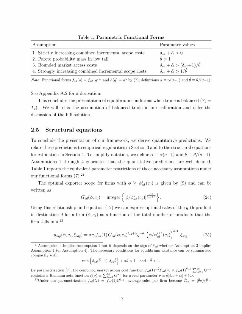
Table 1: Parametric Functional Forms
Assumption Parameter values
1. Strictly increasing combined incremental scope costs δsd + α > 0
2. Pareto probability mass in low tail θ > 1
3. Bounded market access costs δsd + α > (δsd+1)/θ
4. Strongly increasing combined incremental scope costs δsd + α > 1/θ
Note: Functional forms fsd(g) = fsd ·gδsd and h(g) = gα by (7); definitions α ≡ α(σ−1) and θ ≡ θ/(σ−1).
See Appendix A.2 for a derivation.
This concludes the presentation of equilibrium conditions when trade is balanced (Yd =
Td). We will relax the assumption of balanced trade in our calibration and defer the
discussion of the full solution.
2.5 Structural equations
To conclude the presentation of our framework, we derive quantitative predictions. We
relate these predictions to empirical regularities in Section 3 and to the structural equations
for estimation in Section 4. To simplify notation, we define α ≡ α(σ−1) and θ ≡ θ/(σ−1).
Assumptions 1 through 4 guarantee that the quantitative predictions are well defined.
Table 1 reports the equivalent parameter restrictions of those necessary assumptions under
our functional forms (7).21
The optimal exporter scope for firms with φ ≥ φ∗sd (cd) is given by (9) and can be
written as
Gsd(φ, cd) = integer
[φ/φ∗sd (cd)]σ−1
δsd+α
. (24)
Using this relationship and equation (12) we can express optimal sales of the g-th product
in destination d for a firm (φ, cd) as a function of the total number of products that the
firm sells in d:22
ysdg(φ, cd, ξsdg) = σcdfsd(1)Gsd(φ, cd)δsd+αg−α
(φ/φ∗,Gsd (cd)
)σ−1
ξsdg. (25)
21Assumption 4 implies Assumption 1 but it depends on the sign of δsd whether Assumption 3 impliesAssumption 1 (or Assumption 4). The necessary conditions for equilibrium existence can be summarizedcompactly with
minδsd(θ−1), δsdθ
+ αθ > 1 and θ > 1.
By parametrization (7), the combined market access cost function fsd(1)−θFsd(ν) ≡ fsd(1)θ−1∑∞G=1G
−ν
contains a Riemann zeta function ζ(ν) ≡∑∞G=1G
−ν for a real parameter ν ≡ θ[δsd + α] + δsd.22Under our parametrization fsd(G) = fsd(1)Gδsd , average sales per firm become Tsd = [θσ/(θ−
17

Summing over a firm’s products g, we arrive at the firm’s total sales tsd(φ, cd, ξ) =∑g ysdg(φ, cd, ξsdg) and, dividing total sales by exporter scope, we obtain average sales
per product, or average exporter scale. Given (25), exporter scale takes the form
asd(φ, cd, ξ) = σcdfsd(1)Gsd(φ, cd)δsd+α−1
(φ/φ∗,Gsd (cd)
)σ−1
H(Gsd(φ, cd), ξ
)−(σ−1), (26)
where H(Gsd, ξ)−(σ−1) ≡∑Gsd
g=1 g−αξsdg.
3 Data and Regularities
Our Brazilian exporter data originate from all merchandise exports declarations for 2000.
From these customs records we construct a three-dimensional panel of exporters, their
destination countries, and their export products at the Harmonized System (HS) 6-digit
level. In this section, we bring together a set of systematically selected regularities about
multi-product firms and elicit novel aspects of known facts (Eaton et al. 2004; Bernard
et al. 2011; Arkolakis and Muendler 2013). We arrive at these stylized facts guided by
two principles. First, none of the regularities could be generated by mere random shocks
(balls thrown at bins as in Armenter and Koren (2014) would not suffice). Second, the
regularities must characterize the novel extensive margin of product entry (exporter scope)
or the remaining novel intensive margin of sales per product (average exporter scale), or
both, at varying levels of aggregation. These regularities therefore form a body of facts
that any theory of multi-product firms with heterogeneous productivity should match.
We pay particular attention to differences between nearby and far-away destinations to
discipline market access costs.
3.1 Data sources and sample characteristics
Products in the original SECEX (Secretaria de Comercio Exterior) exports data for 2000
are reported using 8-digit codes (under the common Mercosur nomenclature), of which
the first six digits coincide with 6-digit Harmonized System (HS) codes. We aggregate the
data to the HS 6-digit product and firm level so that the resulting dataset is comparable
1)]fsd(1)∑∞G=1G
−δsd(θ−1)h(G)−θ and the access costs fsd(1) can be recovered recursively from
Ts`Tsk
=fs`(1)
fsk(1)
for any pair of destinations ` and k, after normalizing fsd(1) for one destination.
18
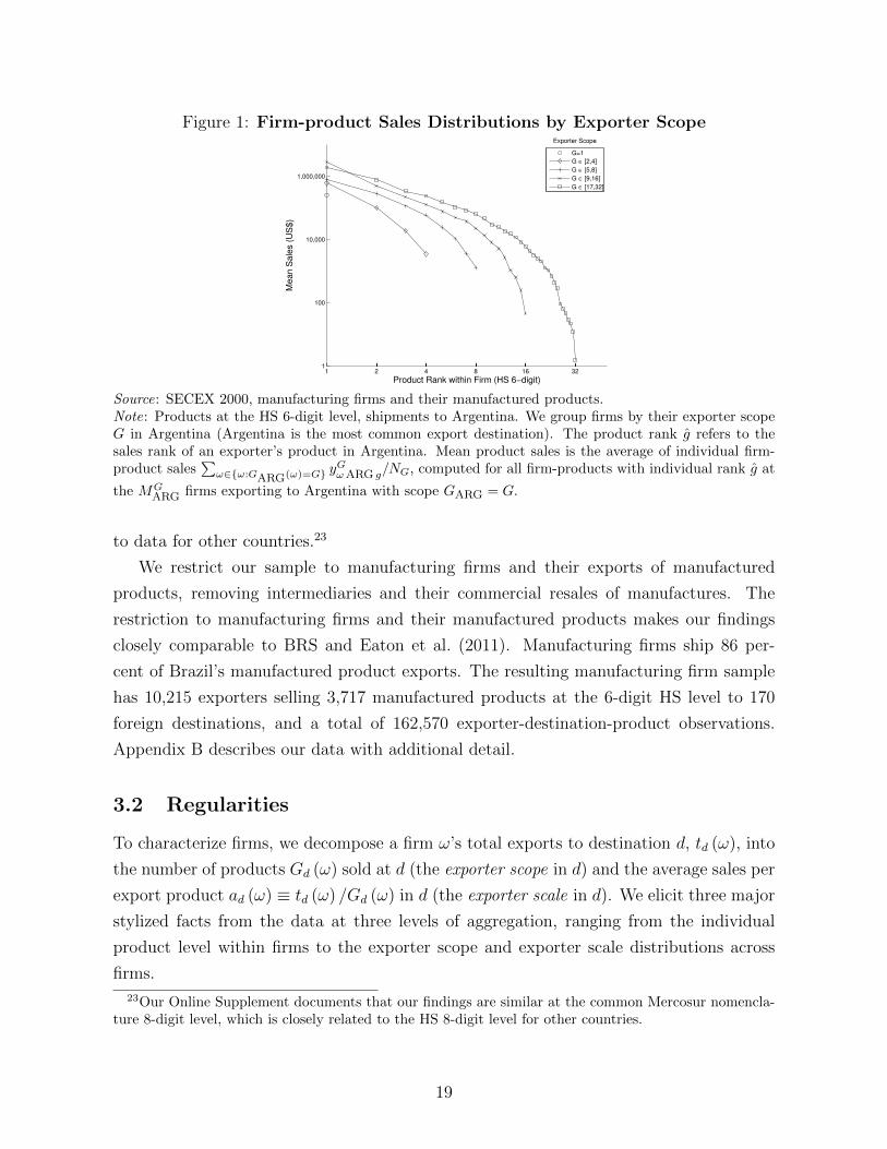
Figure 1: Firm-product Sales Distributions by Exporter Scope
1 2 4 8 16 321
100
10,000
1,000,000
Product Rank within Firm (HS 6−digit)
Mean S
ale
s (
US
$)
G=1
G ∈ [2,4]
G ∈ [5,8]
G ∈ [9,16]
G ∈ [17,32]
Exporter Scope
Source: SECEX 2000, manufacturing firms and their manufactured products.Note: Products at the HS 6-digit level, shipments to Argentina. We group firms by their exporter scopeG in Argentina (Argentina is the most common export destination). The product rank g refers to thesales rank of an exporter’s product in Argentina. Mean product sales is the average of individual firm-product sales
∑ω∈ω:GARG(ω)=G y
GωARG g/NG, computed for all firm-products with individual rank g at
the MGARG firms exporting to Argentina with scope GARG = G.
to data for other countries.23
We restrict our sample to manufacturing firms and their exports of manufactured
products, removing intermediaries and their commercial resales of manufactures. The
restriction to manufacturing firms and their manufactured products makes our findings
closely comparable to BRS and Eaton et al. (2011). Manufacturing firms ship 86 per-
cent of Brazil’s manufactured product exports. The resulting manufacturing firm sample
has 10,215 exporters selling 3,717 manufactured products at the 6-digit HS level to 170
foreign destinations, and a total of 162,570 exporter-destination-product observations.
Appendix B describes our data with additional detail.
3.2 Regularities
To characterize firms, we decompose a firm ω’s total exports to destination d, td (ω), into
the number of products Gd (ω) sold at d (the exporter scope in d) and the average sales per
export product ad (ω) ≡ td (ω) /Gd (ω) in d (the exporter scale in d). We elicit three major
stylized facts from the data at three levels of aggregation, ranging from the individual
product level within firms to the exporter scope and exporter scale distributions across
firms.
23Our Online Supplement documents that our findings are similar at the common Mercosur nomencla-ture 8-digit level, which is closely related to the HS 8-digit level for other countries.
19
Fact 1 Within firms and destinations,
1. wide-scope exporters sell large amounts of their top-selling products, with exports
concentrated in a few products, and
2. wide-scope exporters sell small amounts of their lowest-selling products.
Figure 1 documents this fact. For the figure, we limit our sample to exporters at a
single destination and show only firms that ship at least one product to Argentina (the
most common export destination) and group the exporters by their exporter scope G in
Argentina. Results at other export destinations are similar.24 For each scope group G and
for each product rank g, we then take the average of the log of product sales log yGωARG g for
those firm-products in Argentina. The graph plots the average log product sales against
the log product rank by exporter scope group. The figure shows that a firm’s sales within
a destination are concentrated in a few core products consistent with the core competency
view of EN. In the model, the degree of concentration is regulated by how fast fd(g) and
h(g) change with g (the elasticities δd and α ≡ α(σ−1)). Figure 1 also documents that
wide-scope exporters sell more of their top-selling products than firms with few products.
The model’s equation (25) matches this aspect under Assumption 1.
The product ranking of sales within firms need not be globally deterministic, as fd(g)
and h(g) would suggest, but the local product rankings can differ across destinations in
reality, which we model with product-specific taste shocks similar to BRS. Comparing
ranks across destinations, we can assess the relative importance of core competency versus
product-specific taste shocks: for each given HS 6-digit product that a Brazilian firm sells
in Argentina, we can correlate the firm-product’s rank elsewhere with the firm-product’s
Argentinean rank. We find a correlation coefficient of .785 and a Spearman’s rank corre-
lation coefficient of .860, indicating an important role for core competency.
To assess the first statement of Fact 1 for all export destinations, we regress the log-
arithm of the revenues of the best-selling products yωd1 for firm ω to destination d on
log exporter scope Gωd, discerning effects separately for Latin American and Caribbean
(LAC) and non-LAC destinations and conditional on a firm fixed effect χωIω:
log yωd1 = −0.16(.04)
Id∈LAC + 1.30(.04)
logGωd − 0.18(.05)
Id∈LAC × logGωd + χωIω + εωd.
24We present plots for the United States and Uruguay in Appendix B (Figure B.1). Argentina, theUnited States and Uruguay are the top three destinations in terms of presence of Brazilian manufacturingexporters in 2000.
20

This regression is a version of the model’s equation (25) for a firm’s core product g = 1.
The goodness of fit R2 is .54 (standard error in parentheses clustered at firm level) for 170
destinations and 7,096 firms (46,208 observations). The coefficient estimate on logGωd
shows that sales of the best-selling product increase with an elasticity of 1.3 as exporter
scope in a market widens. However, for LAC destinations, the elasticity is only 1.1 (1.30-
0.18). In light of the model’s equation (25) for g = 1, this coefficient can be interpreted
as an estimate of the sum δLAC + α. This variation by destination is closely related to
our later estimation finding that there are destination-specific elasticities of incremental
market access costs with respect to exporter scope. In subsection 3.3 below, we will assess
the first statement of Fact 1 yet more rigorously and estimate the model’s equation (25)
at the individual product g level (not just for the first product).
The second statement in Fact 1 that wide-scope exporters sell their lowest-ranked
products for small amounts is also consistent with our model’s equation (25). The equation
implies for a firm’s least-selling product g = Gωd that its sales fall with a firm’s scope if and
only if market access costs decline with additional products (δd is negative). The finding is
at odds with models of multi-product firms where product access costs are fixed or absent,
such as BRS or Mayer et al. (2014), and underlies our choice of product-specific market
access costs. The second statement in Fact 1 closely relates to our later simulation result
that falling access costs induce more trade mostly through the entry of new exporters
with their first product, whereas falling barriers to product entry raise trade by less than
similar relative declines in variable trade costs.
To assess the second statement in Fact 1 quantitatively, we regress the lowest-ranked
product’s log sales yωdG on a firm’s log exporter scope Gωd in a destination, conditioning
on fixed effects for firm ω and destination d, and obtain an elasticity of −2.07 under an R2
of .39 (standard error of .02 clustered at firm level) for the same number of observations as
above. The coefficient estimate on logGωd shows that sales of the lowest-selling product
fall with an elasticity of 2.1 as exporter scope at a destination widens. In light of the
model’s equation (25) for g = Gωd, this coefficient can be interpreted as an estimate of
δLAC.
Fact 2 At each destination, there are a few wide-scope and many narrow-scope exporters.
Figure 2 plots average exporter scope in the top five destinations of a region (LAC
or non-LAC) against the percentile of an exporter in terms of scope at the destination.
The median firm, conditional on exporting, only ships one or two products to any given
destination. Within a destination, the exporter scope distribution exhibits a concentration
in the upper tail reminiscent of a Pareto distribution.
21

Figure 2: Exporter Scope Distribution
0 0.1 0.2 0.3 0.4 0.5 0.6 0.7 0.8 0.9 10
5
10
15
20
25
30
35
40
45
50
Percentile of Exporter by Exporter Scope
Exp
ort
er
Sco
pe
(H
S 6
−d
igit)
Latin America and CaribbeanRest of World
Source: SECEX 2000, manufacturing firms and their manufactured products.Note: Products at the HS 6-digit level. The percentile of exporters by scope is calculated within a givendestination. Exporter scope is the corresponding scope for a given percentile averaged across the five mostcommon destinations within each of the two regions (LAC or non-LAC).
The exporter scope distribution varies between destinations. Plotted in open dots is
the average exporter scope at top LAC destinations, and with solid dots the exporter
scope at non-LAC destinations. Brazilian exporters have a wider exporter scope at LAC
destinations than at non-LAC destinations. To quantify the difference in exporter scope
across destinations, we run a simple regression of log exporter scope Gωd on an indicator
for LAC destinations and condition on firm fixed effects χωIω:
logGωd = .35(.02)
Id∈LAC + χωIω + εωd.
The R2 is .55 (standard error in parentheses clustered at firm level) for 170 destinations
and 7,096 firms (46,208 observations). In light of the model’s equation (24), a wider
exporter scope in nearby LAC countries, conditional on the common firm effects across
destinations, is consistent with a lower sum δLAC + α than in the rest of the world, similar
to evidence on the first statement in Fact 1.
Fact 3 Average sales per product (exporter scale) and exporter scope exhibit varying de-
stination-specific degrees of correlation, with the correlation positive and highest in distant
destinations.
On average across destinations, exporter scale is increasing in the number of exported
products. When comparing across destinations, an exporter’s average product sales ex-
hibit a stronger positive correlation with exporter scope in more distant destinations. For
22
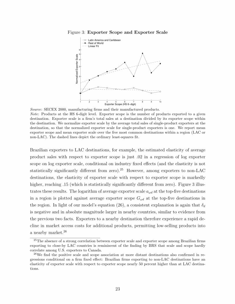
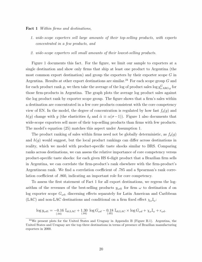
Figure 3: Exporter Scope and Exporter Scale
1 2 3 4 5 6 7 8 9 10
1
2
3
4
5
6
Exporter Scope (HS 6−digit)
No
rma
lize
d E
xp
ort
er
Sca
le
Latin America and CaribbeanRest of WorldLinear Fit
Source: SECEX 2000, manufacturing firms and their manufactured products.Note: Products at the HS 6-digit level. Exporter scope is the number of products exported to a givendestination. Exporter scale is a firm’s total sales at a destination divided by its exporter scope withinthe destination. We normalize exporter scale by the average total sales of single-product exporters at thedestination, so that the normalized exporter scale for single-product exporters is one. We report meanexporter scope and mean exporter scale over the five most common destinations within a region (LAC ornon-LAC). The dashed lines depict the ordinary least-squares fit.
Brazilian exporters to LAC destinations, for example, the estimated elasticity of average
product sales with respect to exporter scope is just .02 in a regression of log exporter
scope on log exporter scale, conditional on industry fixed effects (and the elasticity is not
statistically significantly different from zero).25 However, among exporters to non-LAC
destinations, the elasticity of exporter scale with respect to exporter scope is markedly
higher, reaching .15 (which is statistically significantly different from zero). Figure 3 illus-
trates these results. The logarithm of average exporter scale aωd at the top-five destinations
in a region is plotted against average exporter scope Gωd at the top-five destinations in
the region. In light of our model’s equation (26), a consistent explanation is again that δd
is negative and in absolute magnitude larger in nearby countries, similar to evidence from
the previous two facts. Exporters to a nearby destination therefore experience a rapid de-
cline in market access costs for additional products, permitting low-selling products into
a nearby market.26
25The absence of a strong correlation between exporter scale and exporter scope among Brazilian firmsexporting to close-by LAC countries is reminiscent of the finding by BRS that scale and scope hardlycorrelate among U.S. exporters to Canada.
26We find the positive scale and scope association at more distant destinations also confirmed in re-gressions conditional on a firm fixed effect: Brazilian firms exporting to non-LAC destinations have anelasticity of exporter scale with respect to exporter scope nearly 50 percent higher than at LAC destina-tions.
23

3.3 Scale-scope-rank regression
We conclude our descriptive exploration of the data with an empirical assessment of Fact 1
(Figure 1) at the product level. For this purpose, we simplify the model and set both the
market access cost and the local product appeal to unity across all firms and destinations:
cd = ξdg = 1. Using equation (25), we can express firm ω’s log sales yωdg of the g-th
product in destination d as a function of the firm’s log exporter scope Gωd and the log
local rank of the firm’s product g:
ln yωdg = (δd+ α) lnGωd− α ln g−(1/θ) ln(1−PrGωd)+lnσ[fd(1)/f(1)]Id∈LAC +χωIω+εωdg,
(27)
using the fact that our model implies (σ−1) ln(φω/φ∗,Gd ) = −(1/θ) ln(1−PrGωd) for cd = 1.
To measure 1 − PrGωd, we compute a Brazilian firm’s local sales percentile among the
Brazilian exporters with minimum exporter scope G and include the log percentile as
a regressor. We augment the estimation equation with a combined disturbance χωIω +
εωdg, simply recognizing that the equation will only hold with some empirical error, and
condition out a firm’s worldwide fixed effect χω. The (exhaustive) set of firm effects
absorbs the worldwide average log fixed cost ln σf(1).
There are concerns using estimation equation (27). The equation is misspecified if
local sales shocks ξdg permutate the global rank order of a firm’s products and turn the
order into different location-specific rankings. This misspecification makes the equation
“memoryless” in that estimation does not register a firm-product’s identity across loca-
tions and therefore loses account of the firm-product’s ranking outside a given location
d. Moreover, the estimation equation suffers an omitted variable bias because unobserved
positive firm-destination product appeal shocks will both tend to raise exporter scope
and to systematically permutate the local rank order of firm products; this omitted vari-
able bias would expectedly distort the estimates of δd. To mitigate the concerns, we
estimate equation (27) in two parts by restricting the estimation sample: (i) we isolate
the intercept of the graphs in Figure 1 by restricting the sample just the best selling (or
second-best selling) product, g = 1 (or g = 2), and estimate how the intercept varies with
exporter scope for two location groups Gω,d∈LAC (LAC) and Gω,d∈ROW (non-LAC destina-
tions); (ii) we measure the slope of the graphs in Figure 1 by restricting the sample to
Gω,d∈LAC = Gω,d∈ROW = 2 (or Gω,d = 16). To obtain mutually consistent results from this
two-part estimation, we use the estimated coefficients on Id∈LAC and ln(1−PrGωd) from the
first part (i) as constraints on the second part (ii). Given the potential misspecification
under any pair of restrictions, the regressions merely offer a descriptive exploration of the
24
Table 2: Fit of Individual Product Sales
δLAC δROW α θ δLAC−δROW
Baseline: g = 1; G = 2 -1.82 -1.61 3.04 2.35 -0.21(0.09) (0.11) (0.08) (0.31) (0.10)
Variant 1: g = 2; G = 2 -1.23 -1.13 3.04 2.10 -0.10(0.10) (0.12) (0.08) (0.29) (0.14)
Variant 2: g = 1; G = 16 -1.41 -1.19 2.62 2.35 -0.22(0.11) (0.12) (0.10) (0.31) (0.10)
Source: SECEX 2000, manufacturing firms and their manufactured products.Note: Products at the HS 6-digit level. ols-fe firm fixed effects estimation of equation (27) for firm ω’sindividual product g sales at destination d in two parts, (i) under the baseline restriction g = 1,
ln yωdg = 1.22(0.04)
lnGω,d∈LAC + 1.43(0.07)
lnGω,d∈ROW − 0.43(0.06)
ln(1− PrGωd) − 0.32(0.05)
Id∈LAC + χωIω + εωdg,
and (ii) under the baseline restriction Gωd = 2[ln yωdg − 0.43 ln(1− PrGωd) − 0.32Id∈LAC
]= −3.04
(0.08)ln gωd + χωIω + εωdg.
Robust standard errors from the delta method, clustered at the industry level, in parentheses. Estimatesof δLAC measure the scope elasticity of market access costs for Brazilian firms shipping to other LACdestinations, δROW for Brazilian firms shipping to destinations outside LAC.
data.
Table 2 reports results from the two-part regression exercise under three combinations
of restrictions. The baseline specification uses the restrictions g = 1 and Gωd = 2 for a
pair of regressions under firm fixed effects (standard errors clustered at the level of 259
industries). The first variation uses the restrictions g = 2 and Gωd = 2 for a separate
pair of firm fixed effects regressions and the second variation combines the restrictions
g = 1 and Gωd = 16 for a final pair of firm fixed effects regressions.27 As expected from
the different relationships between exporter scope and scale outside LAC and within LAC
(Figure 3), δLAC exceeds δROW in absolute magnitude. Overall δd falls in the range between
−1.13 and −1.82 across specifications and regions, while α lies in the range from 2.62 to
3.04 and θ between 2.10 and 2.35. In the baseline specification, the magnitudes of the
δd estimates imply that incremental local entry costs drop at an elasticity of −1.61 when
manufacturers introduce additional products in markets outside LAC, and with −1.82
within LAC. But firm-product efficiency drops off even faster with an elasticity of around
3.04 in the basleline. Adding the two fixed scope cost coefficients suggests that there are
27We also explored industry and destination fixed effects regressions in pairs and found results to bebroadly similar.
25
net overall diseconomies of scope with a scope elasticity of 1.22 in LAC and 1.43 in non-
LAC destinations. The coefficient estimates suggest that Assumptions 1 and 2 in Table 1
are satisfied in our data.
Based on these initial descriptive explorations, the power in the partial elasticity ra-
tio (20) is strictly negative across all specifications because we find δd+ α > 0 > δd/θ. The
partial elasticity of trade with respect to an additional product’s fixed cost is therefore
lower than the elasticity with respect to the core product. In other words, these initial
descriptive estimates imply that product entry at multi-product exporters should matter
less than firm entry with the core product. We now turn from descriptive explorations
to an internally consistent estimator and will use the measured parameter magnitudes to
assess the importance of each margin for overall trade.
4 Estimation
We adopt a method of simulated moments for parameter estimation.28 We specify the
product appeal shocks ξdg and the market access costs shocks cd to be distributed log-
normally with mean zero and variance σc and σξ, respectively.
We need to identify five parameters Θ = δ, α, θ, σξ, σc, where α ≡ α(σ−1) and
θ ≡ θ/(σ−1). These five parameters fully characterize the relevant shapes of our func-
tional forms and the dispersion of the three stochastic elements—Pareto distributed firm-
level productivity, the random firm-level market access cost component, and local product
appeal shocks. Our moments are standardized relative to the median firm or top firm-
product at a destination. This produces a simulation estimator invariant to two determin-
istic shifters in the firms’ cost and revenue functions: a destination-specific market access
cost shifter σfd(1) and a destination-specific revenue shifter Dd, which are both common
across exporters at a destination. Moreover, we specify the domestic access cost compo-
nents ξBRA g and cBRA to be deterministic so that every exporter sells in the home market
with certainty. In our ultimate implementation of the simulated moments estimator, we
adopt an extension to destination-specific scope elasticities of market access costs with δd
28The presence of overlaying market access cost and product appeal shocks renders conventional es-timators problematic, as they would involve the numeric evaluation of integrals. Both a firm’s marketaccess cost shock cωd is potentially widely dispersed and a firm-product’s rank gω in production can differfrom the firm-product’s observed local rank in sales (gωd ≡ 1 +
∑Gk=1 1[yωdk(ξdk)>yωdg(ξdg)), especially if
the product appeal shock ξdg is widely dispersed. The implied stochastic permutations of exporter scopesand product ranks introduce an exacting dimensionality that is hard to handle with a maximum likelihoodestimator and the need for numerical computation of higher moments makes a general method of momentsdifficult to implement.
26

varying between LAC and non-LAC countries.
4.1 Moments
At any iteration of the simulation, we use the candidate parameters Θ to compute a sim-
ulated vector of moments msim(Θ), analogous to moments in the data mdata. We use five
sets of simulated moments. Each set is designed to characterize select parameters and to
capture a salient fact from Section 3 or from the literature. However, we exclude moments
related to Fact 3 from our set of targeted moments. Instead, we will use Fact 3 to assess
the fit of our estimates to that regularity after estimation. We now summarize the sim-
ulated moments and discuss how they contribute to parameter identification. Additional
details on the moment definitions as well as the simulation algorithm can be found in
Appendix D.
1. Sales of the top-selling product across firms within destinations. Based on the first
statement of Fact 1, we characterize the top-selling products’ sales across firms with
the same exporter scope. Among firms exporting three or four products to Argentina,
for example, we take the ratio of the top-selling product at the 95th percentile across
firms and the top-selling product of the median firm. Our restriction to the top
product and our standardization by the median firm with the same scope isolate the
stochastic components by equation (25) and therefore help identify the dispersion of
product appeal shocks (and partly the dispersion of the market access cost shock).
2. Within-destination and within-firm product sales concentration. We then use the
second statement in Fact 1 and the ratios between the sales of given lower-ranked
products and the sales of the top product to characterize the concentration of sales
within firms. The comparison of sales within firms neutralizes a firm’s global produc-
tivity ranking and eliminates the role of exporter scope as well as destination-specific
determinants by equation (25). The within-firm within-destination sales ratios there-
fore help pin down the scope elasticity of product efficiency α and help identify the
dispersion of product appeal shocks.
3. Within-destination exporter scope distribution. We then turn to Fact 2 and com-
pute, within destinations, the shares of exporters with certain exporter scopes. For
example, we calculate the proportion of exporters to Argentina, shipping three or
four products. The frequencies of firms with a given exporter scope help identify the
shape parameter θ of the Pareto firm size distribution (and partly the dispersion of
27
the market access cost shock) and help pin down the scope elasticity δ + α, which
translates productivity into exporter scope by equation (24).
4. Market presence combinations. Mirroring similar regularities documented in Eaton
et al. (2011), we use the frequency of firms shipping to any permutation of Brazil’s
top five export destinations in LAC and the top five destinations outside of LAC. For
example, we target the number of exporters that ship to Argentina and Chile, but
not to Bolivia, Paraguay and Uruguay. Matching these market presence patterns
helps us identify the dispersion of market access cost shocks.
5. Within-firm export proportions between destination pairs. It is a widely documented
fact that a firm’s sales are positively correlated across destinations. For each firm,
we pair its total sales to a given destination with its sales to Brazil’s respective
top destination in LAC or outside LAC. The ratio of a firm’s total sales to two
destinations depends on the firm’s respective exporter scopes by equation (26) and
therefore helps pin down the scope elasticity of sales δ+ α. The pairwise sales ratios
also help identify the dispersion of product appeal shocks and market access shocks.
4.2 Inference
Inference proceeds as follows. To find an estimate of Θ, we first stack the differences
between observed and simulated moments ∆m (Θ) = mdata −msim(Θ.
The true parameter Θ0 satisfies E [∆m (Θ0)] = 0, so we search for the Θ that minimizes
the weighted sum of squares, ∆m (Θ)′W∆m (Θ), where W is a positive semi-definite
weighting matrix. Ideally we would obtain W = V−1 where V is the variance-covariance
matrix of the moments. However, the true matrix is unknown, so we use the empirical
analogue:
V =1
N sample
Nsample∑n=1
(mdata −msample
n
) (mdata −msample
n
)′,
where msamplen are the moments from a random sample drawn with replacement of the
original firms in the dataset and N sample is the number of those draws.29 To search for
Θ we use a derivative-free Nelder-Mead downhill simplex search. We compute standard
errors using a bootstrap method that allows for sampling and simulation error.30
29Currently, we use N sample = 1, 000. Due to adding up constrains, we cannot invert this matrix V.Instead, we take a Moore–Penrose pseudo-inverse.
30For the bootstrap we repeat the estimation process 30 times, replacing mdata with mbootstrap sample
to generate standard errors. The bootstrapped standard errors are not centered.
28
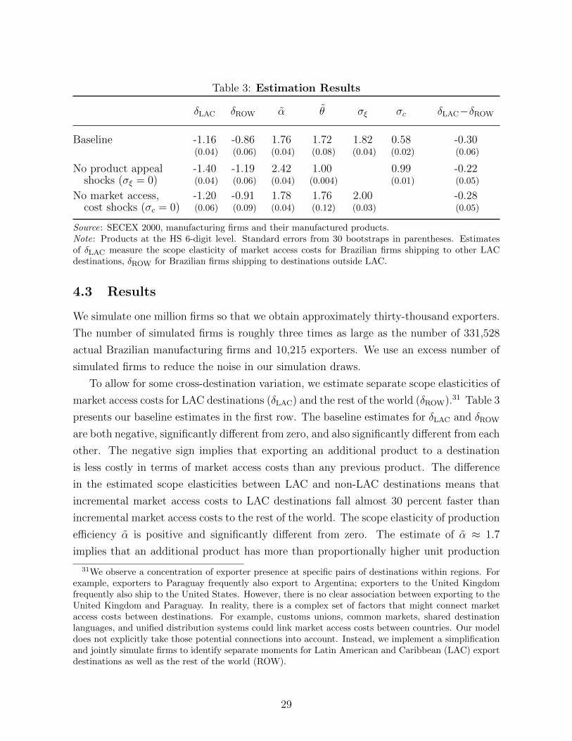
Table 3: Estimation Results
δLAC δROW α θ σξ σc δLAC−δROW
Baseline -1.16 -0.86 1.76 1.72 1.82 0.58 -0.30(0.04) (0.06) (0.04) (0.08) (0.04) (0.02) (0.06)
No product appeal -1.40 -1.19 2.42 1.00 0.99 -0.22shocks (σξ = 0) (0.04) (0.06) (0.04) (0.004) (0.01) (0.05)
No market access, -1.20 -0.91 1.78 1.76 2.00 -0.28cost shocks (σc = 0) (0.06) (0.09) (0.04) (0.12) (0.03) (0.05)
Source: SECEX 2000, manufacturing firms and their manufactured products.Note: Products at the HS 6-digit level. Standard errors from 30 bootstraps in parentheses. Estimatesof δLAC measure the scope elasticity of market access costs for Brazilian firms shipping to other LACdestinations, δROW for Brazilian firms shipping to destinations outside LAC.
4.3 Results
We simulate one million firms so that we obtain approximately thirty-thousand exporters.
The number of simulated firms is roughly three times as large as the number of 331,528
actual Brazilian manufacturing firms and 10,215 exporters. We use an excess number of
simulated firms to reduce the noise in our simulation draws.
To allow for some cross-destination variation, we estimate separate scope elasticities of
market access costs for LAC destinations (δLAC) and the rest of the world (δROW).31 Table 3
presents our baseline estimates in the first row. The baseline estimates for δLAC and δROW
are both negative, significantly different from zero, and also significantly different from each
other. The negative sign implies that exporting an additional product to a destination
is less costly in terms of market access costs than any previous product. The difference
in the estimated scope elasticities between LAC and non-LAC destinations means that
incremental market access costs to LAC destinations fall almost 30 percent faster than
incremental market access costs to the rest of the world. The scope elasticity of production
efficiency α is positive and significantly different from zero. The estimate of α ≈ 1.7
implies that an additional product has more than proportionally higher unit production
31We observe a concentration of exporter presence at specific pairs of destinations within regions. Forexample, exporters to Paraguay frequently also export to Argentina; exporters to the United Kingdomfrequently also ship to the United States. However, there is no clear association between exporting to theUnited Kingdom and Paraguay. In reality, there is a complex set of factors that might connect marketaccess costs between destinations. For example, customs unions, common markets, shared destinationlanguages, and unified distribution systems could link market access costs between countries. Our modeldoes not explicitly take those potential connections into account. Instead, we implement a simplificationand jointly simulate firms to identify separate moments for Latin American and Caribbean (LAC) exportdestinations as well as the rest of the world (ROW).
29

costs than any infra-marginal product. In both the LAC region and the rest of the world,
the combined scope elasticity δd + α is strictly positive and implies strictly increasing
incremental scope costs (Assumption 1 is therefore empirically satisfied). Overall, the
estimates from the simulated method of moments are similar in broad terms to those
from our baseline descriptive data exploration in the preceding section (Table 2) but all
coefficients are smaller in absolute magnitude in the current baseline specification.
Our baseline estimate for θ is statistically significantly above 1 and significantly less
than 2 (Assumption 2 is therefore also empirically satisfied, consistent with a Pareto
distribution of firm productivity). The baseline estimate of the variance of firm-product
appeal shocks σξ is approximately 2 and implies that, conditional on market access cost
shocks and firm productivity, the ratio of the 75th firm sales percentile to the 25th firm
sales percentile is over 10. This large disparity stands in contrast to the implications of
our baseline estimates for σc, which imply that the ratio of the 75th firm sales percentile
to the 25th firm sales percentile is only about 2, far less than 10.32
To explore the implications of our baseline estimates for the sources of variation in
firm-product sales more systematically, we apply a log decomposition to equation (25)33
log yGωdg = −α log gω︸ ︷︷ ︸A
+ (δd + α) logGωd︸ ︷︷ ︸B
+ log cωd + (σ−1) log[φω/φ∗,Gd (cωd)]︸ ︷︷ ︸
C
+ log ξωdg︸ ︷︷ ︸D
.
Our estimates for LAC destinations imply that components A and B, which account for
both a firm-product’s global production rank gω as well as the firm’s local exporter scope
Gωd, explain 34 percent of sales variation. Component C, which reflects the combined mar-
ket access costs shock and productivity for firms with identical exporter product scope,
accounts for 17 percent of sales variation at LAC destinations. Individual firm-product
appeal shocks in component D account for 50 percent of sales variations in LAC coun-
tries. The breakdown is slightly different non-LAC destinations. Components A and B
explain only 21 percent of firm-product sales, component C accounts for 20 percent, and
component D accounts for the remaining 60 percent. This difference between LAC and
non-LAC destinations is entirely due to the difference between δLAC and δROW, which for
LAC destinations augments the importance of exporter scope and reduces the dependence
32Eaton et al. (2011), in a similar model but without multi-product firms and under slightly differentsources of heterogeneity, find θ ≈ 2.5, which is larger than our estimate of 1.72. Their estimate of θcaptures the elasticity of substitution between firms, whereas ours reflects the elasticity of substitutionbetween firm-product varieties. Our estimate for σξ is inline with Eaton et al. (2011) who find that theirfirm-specific appeal shock has a variance of 1.69. However, our appeal shock is firm-product specific (notjust firm specific), so the estimates are not directly comparable.
33We standardize firm-product sales by σfd(1) in estimation.
30

on individual product appeal shocks.
An interpretation of components A and B is that they show firm-level competency
(core competency in a particular firm-product and overall firm capability with regards
to exporter scope), whereas component C reflects idiosyncratic firm heterogeneity, and
component D the randomness of individual product appeal. Product appeal shocks play a
dominant role in firm sales. However, the combination of firm-level competency and firm
heterogeneity plays nearly as important a part. Our estimates highlight that a reduction
in the scope elasticity of incremental market access costs from their magnitude in non-
LAC countries to the magnitude in LAC countries raises the importance of firm-level
competency considerably.
In two departures from our baseline specification, we re-estimate the model dropping
one source of heterogeneity at a time: we first omit product appeal shocks and then drop
market access cost shocks. We report the resulting estimates in the second and third
row of Table 3. When we omit product appeal shocks (setting σξ = 0), the estimated
dispersion of market access costs expectedly increases. In addition, the estimated mag-
nitudes of the scope elasticities δd and α markedly increase. The estimate of the shape
parameter of the Pareto firm size distribution ˆθ hits a corner solution (and barely satisfies
Assumption 2). Those salient changes in parameter estimates underscore the importance
of specifying product appeal shocks. Interestingly, however, the regional difference in the
scope elasticity of market access costs δLAC − δROW remains similar to that under our
our baseline estimates. Dropping market access cost shocks has only minor effects on the
remaining estimates.34
Relating our results back to the findings from Table 2, which were based on simple log
linear estimators dropping both sources of heterogeneity (product appeal shocks and mar-
ket access cost shocks), we find qualitatively similar results. This broad similarity across
estimators suggests that both simulated method of moments and its simpler counterparts
identify comparable principal variation in the data but the quantitative differences indicate
the importance of heterogeneity in the product appeal and market access costs.
To assess the sensitivity of our results to potential heterogeneity in product types and
heterogeneity in destinations, we repeat estimation for numerous alternative specifications:
we demean firm-product sales at the HS 6-digit level by average Brazilian exports at the
HS 2-digit level, we restrict the sample to firms in high-tech manufacturing industries,
34We cannot compare the goodness of fit in meaningful ways across specifications because the momentsused under the restrictions differ from the baseline estimation. For σξ = 0, we have to limit the set ofmoments 2 to the median because there is no variation by percentile in the simulation. For σc = 0, wehave to exclude the set of moments 4 and 5.
31
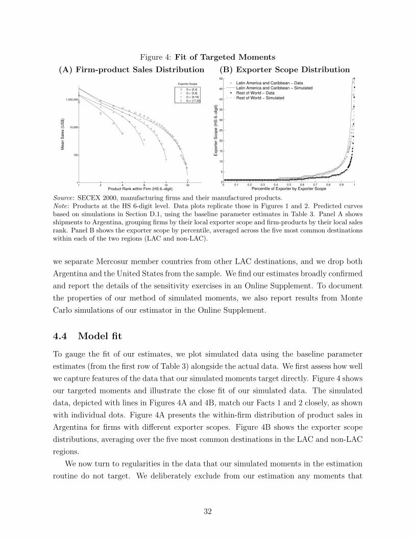
Figure 4: Fit of Targeted Moments
(A) Firm-product Sales Distribution (B) Exporter Scope Distribution
1 2 4 8 16 321
100
10,000
1,000,000
Product Rank within Firm (HS 6−digit)
Me
an
Sa
les (
US
$)
G ∈ [2,4]
G ∈ [5,8]
G ∈ [9,16]
G ∈ [17,32]
Exporter Scope
0 0.1 0.2 0.3 0.4 0.5 0.6 0.7 0.8 0.9 10
5
10
15
20
25
30
35
40
45
50
Percentile of Exporter by Exporter Scope
Exp
ort
er
Sco
pe
(H
S 6
−d
igit)
Latin America and Caribbean − DataLatin America and Caribbean − SimulatedRest of World − DataRest of World − Simulated
Source: SECEX 2000, manufacturing firms and their manufactured products.Note: Products at the HS 6-digit level. Data plots replicate those in Figures 1 and 2. Predicted curvesbased on simulations in Section D.1, using the baseline parameter estimates in Table 3. Panel A showsshipments to Argentina, grouping firms by their local exporter scope and firm-products by their local salesrank. Panel B shows the exporter scope by percentile, averaged across the five most common destinationswithin each of the two regions (LAC and non-LAC).
we separate Mercosur member countries from other LAC destinations, and we drop both
Argentina and the United States from the sample. We find our estimates broadly confirmed
and report the details of the sensitivity exercises in an Online Supplement. To document
the properties of our method of simulated moments, we also report results from Monte
Carlo simulations of our estimator in the Online Supplement.
4.4 Model fit
To gauge the fit of our estimates, we plot simulated data using the baseline parameter
estimates (from the first row of Table 3) alongside the actual data. We first assess how well
we capture features of the data that our simulated moments target directly. Figure 4 shows
our targeted moments and illustrate the close fit of our simulated data. The simulated
data, depicted with lines in Figures 4A and 4B, match our Facts 1 and 2 closely, as shown
with individual dots. Figure 4A presents the within-firm distribution of product sales in
Argentina for firms with different exporter scopes. Figure 4B shows the exporter scope
distributions, averaging over the five most common destinations in the LAC and non-LAC
regions.
We now turn to regularities in the data that our simulated moments in the estimation
routine do not target. We deliberately exclude from our estimation any moments that
32
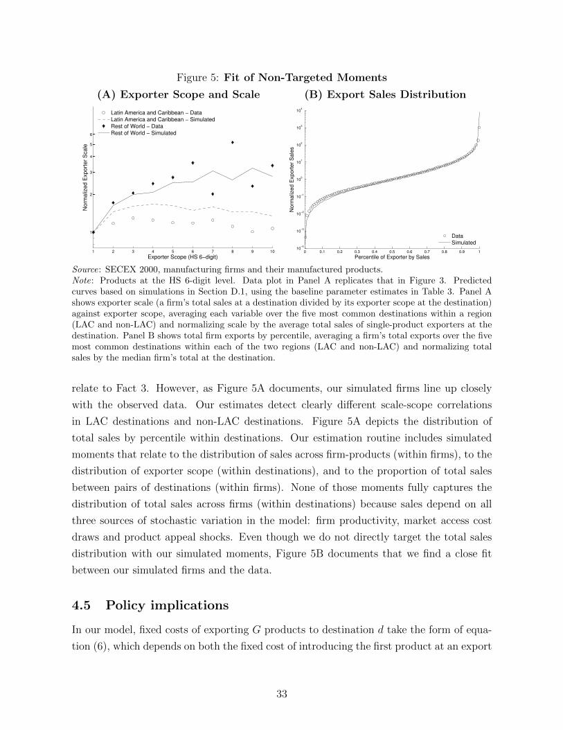
Figure 5: Fit of Non-Targeted Moments
(A) Exporter Scope and Scale (B) Export Sales Distribution
1 2 3 4 5 6 7 8 9 10
1
2
3
4
5
6
Exporter Scope (HS 6−digit)
No
rma
lize
d E
xp
ort
er
Sca
le
Latin America and Caribbean − DataLatin America and Caribbean − SimulatedRest of World − DataRest of World − Simulated
0 0.1 0.2 0.3 0.4 0.5 0.6 0.7 0.8 0.9 110
−4
10−3
10−2
10−1
100
101
102
103
104
Percentile of Exporter by Sales
No
rma
lize
d E
xp
ort
er
Sa
les
DataSimulated
Source: SECEX 2000, manufacturing firms and their manufactured products.Note: Products at the HS 6-digit level. Data plot in Panel A replicates that in Figure 3. Predictedcurves based on simulations in Section D.1, using the baseline parameter estimates in Table 3. Panel Ashows exporter scale (a firm’s total sales at a destination divided by its exporter scope at the destination)against exporter scope, averaging each variable over the five most common destinations within a region(LAC and non-LAC) and normalizing scale by the average total sales of single-product exporters at thedestination. Panel B shows total firm exports by percentile, averaging a firm’s total exports over the fivemost common destinations within each of the two regions (LAC and non-LAC) and normalizing totalsales by the median firm’s total at the destination.
relate to Fact 3. However, as Figure 5A documents, our simulated firms line up closely
with the observed data. Our estimates detect clearly different scale-scope correlations
in LAC destinations and non-LAC destinations. Figure 5A depicts the distribution of
total sales by percentile within destinations. Our estimation routine includes simulated
moments that relate to the distribution of sales across firm-products (within firms), to the
distribution of exporter scope (within destinations), and to the proportion of total sales
between pairs of destinations (within firms). None of those moments fully captures the
distribution of total sales across firms (within destinations) because sales depend on all
three sources of stochastic variation in the model: firm productivity, market access cost
draws and product appeal shocks. Even though we do not directly target the total sales
distribution with our simulated moments, Figure 5B documents that we find a close fit
between our simulated firms and the data.
4.5 Policy implications
In our model, fixed costs of exporting G products to destination d take the form of equa-
tion (6), which depends on both the fixed cost of introducing the first product at an export
33
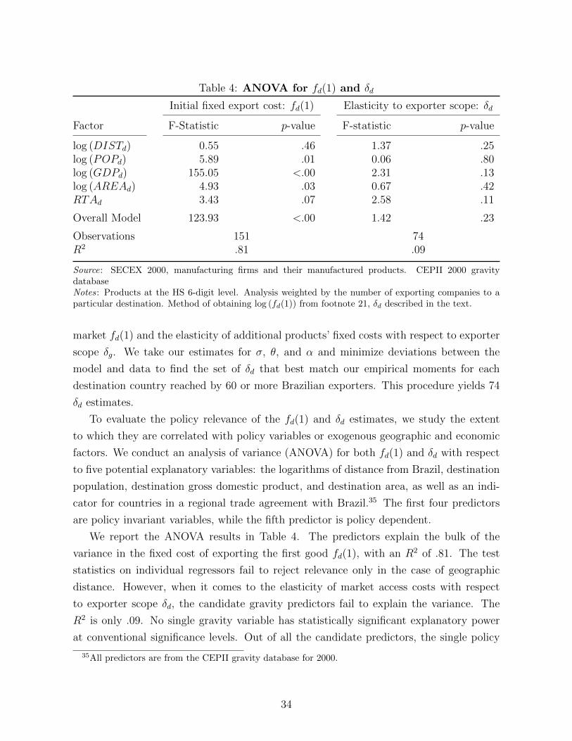
Table 4: ANOVA for fd(1) and δd
Initial fixed export cost: fd(1) Elasticity to exporter scope: δd
Factor F-Statistic p-value F-statistic p-value
log (DISTd) 0.55 .46 1.37 .25log (POPd) 5.89 .01 0.06 .80log (GDPd) 155.05 <.00 2.31 .13log (AREAd) 4.93 .03 0.67 .42RTAd 3.43 .07 2.58 .11
Overall Model 123.93 <.00 1.42 .23
Observations 151 74R2 .81 .09
Source: SECEX 2000, manufacturing firms and their manufactured products. CEPII 2000 gravitydatabaseNotes: Products at the HS 6-digit level. Analysis weighted by the number of exporting companies to aparticular destination. Method of obtaining log (fd(1)) from footnote 21, δd described in the text.
market fd(1) and the elasticity of additional products’ fixed costs with respect to exporter
scope δg. We take our estimates for σ, θ, and α and minimize deviations between the
model and data to find the set of δd that best match our empirical moments for each
destination country reached by 60 or more Brazilian exporters. This procedure yields 74
δd estimates.
To evaluate the policy relevance of the fd(1) and δd estimates, we study the extent
to which they are correlated with policy variables or exogenous geographic and economic
factors. We conduct an analysis of variance (ANOVA) for both fd(1) and δd with respect
to five potential explanatory variables: the logarithms of distance from Brazil, destination
population, destination gross domestic product, and destination area, as well as an indi-
cator for countries in a regional trade agreement with Brazil.35 The first four predictors
are policy invariant variables, while the fifth predictor is policy dependent.
We report the ANOVA results in Table 4. The predictors explain the bulk of the
variance in the fixed cost of exporting the first good fd(1), with an R2 of .81. The test
statistics on individual regressors fail to reject relevance only in the case of geographic
distance. However, when it comes to the elasticity of market access costs with respect
to exporter scope δd, the candidate gravity predictors fail to explain the variance. The
R2 is only .09. No single gravity variable has statistically significant explanatory power
at conventional significance levels. Out of all the candidate predictors, the single policy
35All predictors are from the CEPII gravity database for 2000.
34
variable—the indicator for a regional trade agreement with Brazil RTAd—comes closest to
conventional statistical significance. In a final exercise, we estimate the correlation between
our market access cost measure for Brazilian exporters and the ad-valorem equivalent NTM
measures in Kee et al. (2009) for a comparison. Corroborating the complementary nature
of our approach, our firm-product market access cost estimates for additional products are
significantly positively correlated with the ad-valorem equivalent NTM measures by Kee
et al. (2009), when existent, with a correlation coefficient of about one-half for destinations
with at least 200 Brazilian exporters.
Taken together these findings provide evidence consistent with the hypothesis that
exogenous geography related, and therefore policy invariant, factors play no statistically
relevant role for the determination of the elasticity of incremental market access costs
δd, in contrast with the usual specification of fixed market access costs fd(1). Previous
estimates of policy relevant NTMs, however, are significantly positively related to our
market access cost estimates for additional products. We therefore maintain the tenet
that market related economic determinants, amenable to policy, plausibly shape δd and
proceed to study the impact of reducing related market access barriers.
5 General Equilibrium Counterfactual
We conduct a counterfactual simulation to quantify the implied impact of our baseline
estimates (first row of Table 3) for changes to bilateral trade when destination-specific
market access costs are brought down. Brazil is close to the median country in exports
per capita, so we consider our baseline parameter estimates informative for global trade.36
Our main counterfactual exercise harmonizes market access cost schedules across destina-
tions. We reduce the market access cost for an additional product (not counting a firm’s
first product) at distant destinations to the level at nearby destinations. In a broad sense,
this exercise helps apprise the importance of multi-product exporters when it comes to the
reduction of market access costs for additional products. Examples of relevant market ac-
cess costs for additional products are health regulations and safety standards, certifications
and licenses.
To perform the counterfactual experiments, we add three elements to the model fol-
lowing Eaton et al. (2011). (i) We introduce intermediate inputs as in Eaton and Kortum
(2002). In particular, we assume that the production of each product uses a Cobb-Douglas
36By the WTF and WDI data for all industries and countries, Brazil ranks at the 48th percentile (top100th country out of 192) in terms of exports per capita in 2000. Brazil’s total exports in 2000 are at the88th percentile worldwide (top 27th country out of 205).
35

Table 5: Percentage Change in Simulated Welfare (θ = 2.59)
Counterfactual Counterfactual
(1) (2) (3) (4) (1) (2) (3) (4)
Country ∆f(g) ∆f(g)C ∆δ ∆δC Country ∆f(g) ∆f(g)C ∆δ ∆δC
Armenia 0.75 0.51 0.84 0.57 Kuwait 2.68 1.52 2.99 1.69
Australia 1.29 0.76 1.44 0.85 Kyrgyzstan 1.46 0.88 1.63 0.98
Austria 2.72 0.71 3.03 0.80 Latvia 2.14 0.43 2.38 0.49
Azerbaijan 1.31 0.69 1.47 0.77 Lithuania 2.12 0.46 2.37 0.52
BelgmLuxNthl 3.82 1.37 4.26 1.53 Malta 5.30 2.27 5.92 2.54
Bolivia 1.09 0.58 1.22 0.64 Mexico 2.62 0.54 2.91 0.60
Brazil 0.68 0.64 0.76 0.71 Morocco 1.61 1.50 1.80 1.67
Bulgaria 1.95 0.68 2.17 0.76 Norway 1.88 0.59 2.10 0.66
Canada 2.83 0.49 3.16 0.55 Oman 2.74 2.80 3.06 3.12
Chile 1.52 1.39 1.70 1.56 Poland 1.91 0.57 2.13 0.64
ChinaHKG 1.78 1.06 1.99 1.19 Portugal 2.13 0.50 2.38 0.56
Colombia 0.88 0.80 0.98 0.89 Romania 2.15 0.64 2.40 0.71
CostaRica 0.66 0.43 0.74 0.48 RussianFed 2.20 1.15 2.45 1.28
Cyprus 2.95 1.38 3.29 1.54 Senegal 1.52 1.16 1.70 1.29
Ethiopia 0.81 0.60 0.90 0.67 Slovenia 3.50 0.93 3.90 1.04
Finland 2.21 0.76 2.46 0.85 SouthKorea 1.89 1.02 2.11 1.14
FranceMonaco 1.77 0.61 1.97 0.68 Spain 1.73 0.50 1.93 0.56
Germany 1.93 0.79 2.15 0.88 SriLanka 0.76 0.26 0.85 0.30
Hungary 4.68 1.32 5.22 1.47 Sweden 2.02 0.71 2.26 0.80
IndMalSgThai 5.10 2.98 5.68 3.32 TrinidadTbg 0.67 0.32 0.75 0.36
India 2.09 1.35 2.34 1.51 Tunisia 2.73 2.60 3.05 2.90
Iran 0.15 0.06 0.17 0.07 Turkey 1.23 1.02 1.37 1.14
Ireland 5.03 1.99 5.60 2.23 UK 1.62 0.76 1.81 0.85
Israel 1.64 1.35 1.83 1.51 USA 0.89 0.59 0.99 0.66
Italy 1.49 0.52 1.66 0.58 Ukraine 1.68 0.46 1.87 0.51
Japan 0.50 0.32 0.56 0.35 Uruguay 0.97 0.68 1.09 0.75
Jordan 1.80 1.17 2.01 1.30 VietNam 2.58 0.79 2.88 0.88
Kazakhstan 2.04 1.46 2.27 1.63 Yemen 1.05 0.57 1.17 0.64
Kenya 1.31 1.02 1.46 1.13 RestOfWorld 4.73 4.94 5.28 5.51
Mean 2.02 1.02 2.26 1.13
Note: Counterfactual experiments (1) and (3) reduce market access costs everywhere, experiments (2) and (4)reduce market access costs only at destinations outside a source country’s own continent, with ROW treated asa different continent. Experiments use baseline parameter estimates of Θ = δ, α, θ = −1.16, 1.76, 1.72 (seeTable 3). Pareto shape parameter θ = 2.59 imputed from Crozet and Koenig (2010) and estimates in Table 3.See Appendix B.2 for data construction. Following Dekle, Eaton and Kortum (2007), we collapse (i) HongKong, Macao and mainland China, (ii) Belgium, Luxembourg and the Netherlands, (iii) Indonesia, Malaysia,Singapore, and Thailand and (iv) France and Monaco into single markets.
36
aggregate of labor and a composite of all other manufactured products with cost Pd. The
labor share in manufacturing production is β, and the share of intermediate inputs 1−β.
The total input cost is therefore wd = W βd P
1−βd , where we now think of wd as the input
cost and Wd as the wage. (ii) There is a non-manufacturing sector in each country as
in Alvarez and Lucas (2007) that combines manufactures with labor, in a Cobb-Douglas
production function, where manufactures have a share γ in GDP. The price of final output
in country d is proportional to P γdW
1−γd . We state the resulting equations in Appendix A.
(iii) We allow for a manufacturing trade deficit Bd, and for an overall trade deficit BTd in
goods and services. Both deficits are set to their observed levels in 2000.
We compute the share of manufacturing in GDP for each country using data on GDP,
manufacturing production and trade (as described in Appendix B.2). We set the labor
share in manufacturing production to β = .330, the sample average for countries with
available information (Appendix B.2). To compute the impact of a counterfactual change
in market access costs, we use the Dekle et al. (2007) methodology (details in Appendix E).
The merit of this method is that it requires no information on the initial level of technology,
iceberg trade costs, and market access costs. Instead, we can compute the changes in all
equilibrium variables using the percentage change in the underlying parameter of interest
(market access cost parameters in our case).
For our primary results we consider a baseline value of θ = 2.59 from Crozet and
Koenig (2010), which we obtain by averaging across 34 industries.37 For all other starting
parameter values, we use our baseline estimates from row 1 in Table 3.
5.1 Changes in total market access costs
We initially decrease all market access costs for all products (fd) by 15 percent to all inter-
national destinations. In this and all following experiments, we do not change any domestic
trade costs and set the change in total domestic access costs to Fss = 1. Table 5 shows
the results of the counterfactual exercise in terms of changes in welfare (see Appendix E
for derivations). The results of the first experiment are labeled as counterfactual (1) in
Table 5.
In a second experiment, we reduce market access costs only to countries not on the
same continent by 15 percent. The results are shown as counterfactual (2) in Table 5.
37Crozet and Koenig (2010) obtain results for σ, we obtain θ using our estimated value for θ. Eaton etal. (2011) find an estimate of θ = 4.87. In a related set of models, Eaton and Kortum (2002), Bernard,Eaton, Jensen and Kortum (2003) and Simonovska and Waugh (2014) find estimates of θ between 3.60and 8.28.
37
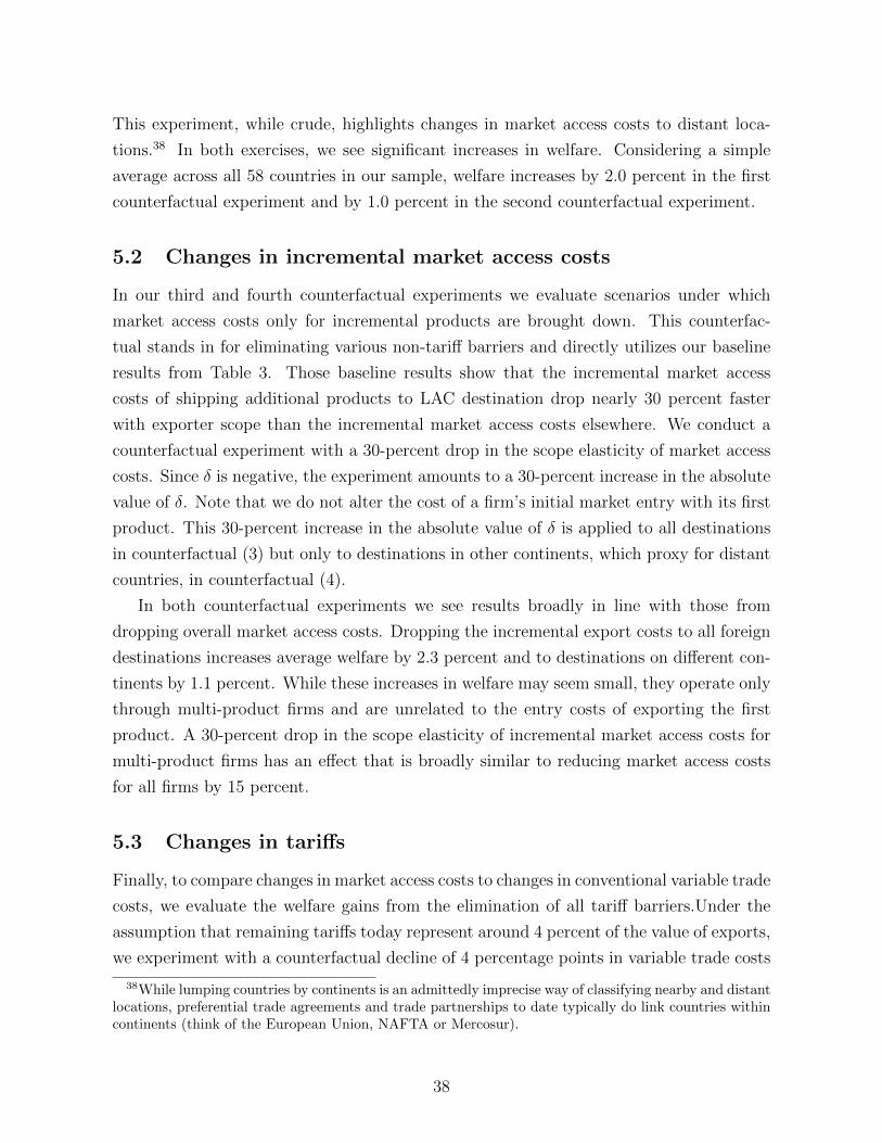
This experiment, while crude, highlights changes in market access costs to distant loca-
tions.38 In both exercises, we see significant increases in welfare. Considering a simple
average across all 58 countries in our sample, welfare increases by 2.0 percent in the first
counterfactual experiment and by 1.0 percent in the second counterfactual experiment.
5.2 Changes in incremental market access costs
In our third and fourth counterfactual experiments we evaluate scenarios under which
market access costs only for incremental products are brought down. This counterfac-
tual stands in for eliminating various non-tariff barriers and directly utilizes our baseline
results from Table 3. Those baseline results show that the incremental market access
costs of shipping additional products to LAC destination drop nearly 30 percent faster
with exporter scope than the incremental market access costs elsewhere. We conduct a
counterfactual experiment with a 30-percent drop in the scope elasticity of market access
costs. Since δ is negative, the experiment amounts to a 30-percent increase in the absolute
value of δ. Note that we do not alter the cost of a firm’s initial market entry with its first
product. This 30-percent increase in the absolute value of δ is applied to all destinations
in counterfactual (3) but only to destinations in other continents, which proxy for distant
countries, in counterfactual (4).
In both counterfactual experiments we see results broadly in line with those from
dropping overall market access costs. Dropping the incremental export costs to all foreign
destinations increases average welfare by 2.3 percent and to destinations on different con-
tinents by 1.1 percent. While these increases in welfare may seem small, they operate only
through multi-product firms and are unrelated to the entry costs of exporting the first
product. A 30-percent drop in the scope elasticity of incremental market access costs for
multi-product firms has an effect that is broadly similar to reducing market access costs
for all firms by 15 percent.
5.3 Changes in tariffs
Finally, to compare changes in market access costs to changes in conventional variable trade
costs, we evaluate the welfare gains from the elimination of all tariff barriers.Under the
assumption that remaining tariffs today represent around 4 percent of the value of exports,
we experiment with a counterfactual decline of 4 percentage points in variable trade costs
38While lumping countries by continents is an admittedly imprecise way of classifying nearby and distantlocations, preferential trade agreements and trade partnerships to date typically do link countries withincontinents (think of the European Union, NAFTA or Mercosur).
38

to mimic the elimination of tariffs.39 Using our parameter estimates, we find an average
welfare gain across markets of approximately 1.8 percent; this is broadly comparable to
the gains from reductions in incremental market access costs.
Our estimate of θ = 2.59 comes from French firm level data used by Crozet and Koenig
(2010). Alternatively, we can use Simonovska and Waugh (2014), who aggregate trade
flows from 123 countries. Their various estimates of θ range from 2.79 to 4.46, with their
preferred specification producing θ = 4.41. Using that latter estimate, our counterfactual
experiment (4), in which we reduce only trade costs to distant destinations, results in
an average welfare increase of 0.8 percent across destinations. Similarly, eliminating all
tariffs increases welfare by 1.7 percent. In summary, our counterfactual experiments with
plausible reductions of market access costs result in welfare gains of a similar magnitude
as the elimination of remaining tariffs.
6 Conclusion
We develop a model that accounts for pertinent facts on multi-product exporters, which we
document using Brazilian exporting micro-data. The model allows us to estimate market
access costs that regulate the entry of exporters and their products, and are important
elements in trade theories with heterogeneous firms. Our estimates indicate that additional
products farther from a firm’s core competency incur higher unit costs but also that the
elasticity of market access costs with respect to additional products declines at an almost
one-third faster rate in nearby destinations. We conduct counterfactual exercises that
accordingly reduce the scope elasticity of market access costs by one-third and find welfare
gains similar in magnitude to a complete elimination of currently remaining tariffs. Results
of these counterfactual exercises are reminiscent of surveys for numerous countries (OECD
2005, Ch. 1) and evidence on product trade (Reyes 2011), which suggest that non-tariff
measures deter the market access of small and narrow-scope firms more heavily.
While we have incorporated many available dimensions of the trade data, more can be
done. Our approach leaves unexplored recently available information on unit prices and
time series trends, for example. Such additional information may prove valuable in under-
standing more precisely the patterns of product market access and exporter expansions.
Similarly, we leave specific mechanisms that may shape market access cost determinants
open for further investigation.
39Novy (2013) finds that the average total variable trade costs for a set of OECD countries in terms oftariff equivalents is 94 percent in 2000; the same countries have ad-valorem tariff rates of approximately4 percent (Anderson and Neary 2005).
39

References
Allanson, Paul and Catia Montagna, “Multiproduct Firms and Market Structure: AnExplorative Application to the Product Life Cycle,” International Journal of Industrial Orga-nization, September 2005, 23 (7-8), 587–97.
Alvarez, Fernando and Robert E. Jr.. Lucas, “General Equilibrium Analysis of the Eaton-Kortum Model of International Trade,” Journal of Monetary Economics, September 2007, 54(6), 1726–68.
Alvarez, Roberto, Hasan Faruq, and Ricardo A. Lopez, “Is Previous Export ExperienceImportant for New Exports?,” Journal of Development Studies, 2013, 49 (3), 426–441.
Amador, Joao and Luca David Opromolla, “Product and Destination Mix in Export Mar-kets,” Review of World Economics/Weltwirtschaftliches Archiv, March 2013, 149 (1), 23–53.
Anderson, James E. and J. Peter Neary, “A New Approach to Evaluating Trade Policy,”Review of Economic Studies, January 1996, 63 (1), 107–25.
and , “The Mercantilist Index of Trade Policy,” International Economic Review, May 2003,44 (2), 627–49.
and , Measuring the Restrictiveness of International Trade Policy, Cambridge and London:MIT Press, 2005.
Arkolakis, Costas, “Market Penetration Costs and the New Consumers Margin in InternationalTrade,” Journal of Political Economy, 2010, 118 (6), 1151–1199.
and Marc-Andreas Muendler, “The Extensive Margin of Exporting Products: The Con-tinuum Case,” University of California, San Diego, unpublished manuscript, 2010.
and , “Exporters and Their Products: A Collection of Empirical Regularities,” CESifoEconomic Studies, June 2013, 59 (2), 223–48.
, Arnaud Costinot, and Andres Rodriguez-Clare, “New Trade Models, Same OldGains?,” American Economic Review, February 2012, 102 (1), 94–130.
, Sharat Ganapati, and Marc-Andreas Muendler, “The Extensive Margin of ExportingProducts: A Firm-level Analysis,” April 2015. Yale University, unpublished manuscript (earlierversion NBER Working Paper, 16641).
Armenter, Roc and Miklos Koren, “A Balls-and-Bins Model of Trade,” American EconomicReview, 2014, 104 (7), 2127–51.
Atkeson, Andrew and Ariel Burstein, “Pricing-to-Market, Trade Costs, and InternationalRelative Prices,” American Economic Review, December 2008, 98 (5), 1998–2031.
Bernard, Andrew B., J. Bradford Jensen, and Peter K. Schott, “Importers, Exportersand Multinationals: A Portrait of Firms in the US That Trade Goods,” in “Producer dynamics:New evidence from micro data,” University of Chicago Press, 2009, pp. 513–552.
40

, Jonathan Eaton, J. Bradford Jensen, and Samuel Kortum, “Plants and Productivityin International Trade,” American Economic Review, 2003, 93 (4), 1268–1290.
, Stephen J. Redding, and Peter K. Schott, “Multiple-Product Firms and ProductSwitching,” American Economic Review, 2010, 100 (1), 70–97.
, , and , “Multiproduct Firms and Trade Liberalization,” Quarterly Journal of Eco-nomics, August 2011, 126 (3), 1271–1318.
Brambilla, Irene, “Multinationals, Technology, and the Introduction of Varieties of Goods,”Journal of International Economics, September 2009, 79 (1), 89–101.
Broda, Christian and David E. Weinstein, “Globalization and the Gains From Variety,”Quarterly Journal of Economics, 2006, 121 (2), 541–585.
Chaney, Thomas, “Distorted Gravity: The Intensive and Extensive Margins of InternationalTrade,” American Economic Review, September 2008, 98 (4), 1707–21.
Comtrade, Commodity Trade Statistics Database, United Nations Statistics Division, 2011.
Crozet, Matthieu and Pamina Koenig, “Structural Gravity Equations with Intensive andExtensive Margins,” Canadian Journal of Economics, February 2010, 43 (1), 41–62.
Dekle, Robert, Jonathan Eaton, and Samuel Kortum, “Unbalanced Trade,” AmericanEconomic Review, May 2007, 97 (2), 351–55.
Dhingra, Swati, “Trading Away Wide Brands for Cheap Brands,” American Economic Review,October 2013, 103 (6), 2554–84.
Eaton, Jonathan and Samuel Kortum, “Technology, Geography, and Trade,” Econometrica,September 2002, 70 (5), 1741–1779.
and , “Technology in the Global Economy: A Framework for Quantitative Analysis,” 2010.University of Chicago, unpublished manuscript.
, , and Francis Kramarz, “Dissecting Trade: Firms, Industries, and Export Destina-tions,” American Economic Review, May 2004, 94 (2), 150–154.
, , and , “An Anatomy of International Trade: Evidence From French Firms,” Econo-metrica, 09 2011, 79 (5), 1453–1498.
Eckel, Carsten and J. Peter Neary, “Multi-product Firms and Flexible Manufacturing inthe Global Economy,” Review of Economic Studies, January 2010, 77 (1), 188–217.
, Leonardo Iacovone, Beata Javorcik, and J. Peter Neary, “Multi-product firms athome and away: Cost- versus quality-based competence,” Journal of International Economics,2015, 95 (2), 216–232.
Feenstra, Robert and Hong Ma, “Optimal Choice of Product Scope for Multiproduct Firms,”in Elhanan Helpman, Dalia Marin, and Thierry Verdier, eds., The Organization of Firms ina Global Economy, Cambridge: Harvard University Press, 2008, chapter 6, pp. 173–199.
41

Feenstra, Robert C., “Estimating the Effects of Trade Policy,” in Gene M. Grossman andKenneth Rogoff, eds., Handbook of International Economics, Vol. 3 of Handbooks in Economics,Amsterdam, New York and Oxford: Elsevier, North-Holland, 1995, pp. 1553–95.
, Robert E. Lipsey, Haiyan Deng, Alyson C. Ma, and Hengyong Mo, “World TradeFlows: 1962-2000,” NBER Working Paper, 2005, 11040.
Goldberg, Pinelopi Koujianou, Amit Kumar Khandelwal, Nina Pavcnik, and PetiaTopalova, “Imported Intermediate Inputs and Domestic Product Growth: Evidence fromIndia,” Quarterly Journal of Economics, November 2010, 125 (4), 1727–1767.
Helpman, Elhanan, Marc J. Melitz, and Stephen R. Yeaple, “Export versus FDI withHeterogeneous Firms,” American Economic Review, March 2004, 94 (1), 300–316.
Hottman, Colin, Stephen J Redding, and David E Weinstein, “What is Firm Het-erogeneity in Trade Models? The Role of Quality, Scope, Markups, and Cost,” Unpublishedmanuscript, 2014.
Iacovone, Leonardo and Beata Javorcik, “Shipping Good Tequila Out: Investment, Do-mestic Unit Values and Entry of Multi-Product Plants Into Export Markets,” Unpublishedmanuscript, 2008.
Kee, Hiau Looi, Alessandro Nicita, and Marcelo Olarreaga, “Estimating Trade Restric-tiveness Indices,” Economic Journal, January 2009, 119 (534), 172–99.
Mayer, Thierry, Marc J. Melitz, and Gianmarco I. P. Ottaviano, “Market Size, Compe-tition, and the Product Mix of Exporters,” American Economic Review, February 2014, 104(2), 495–536.
McKenzie, Lionel W., “Matrices with Dominant Diagonal in Economic Theory,” in K. J.Arrow, S. Karlin, and P. Suppes, eds., Mathematical Methods in the Social Sciences, 1959:Proceedings of the first Stanford symposium, Palo Alto: Stanford University Press, 1960, chap-ter 2, p. 4762.
Melitz, Marc J., “The Impact of Trade on Intra-industry Reallocations and Aggregate IndustryProductivity,” Econometrica, November 2003, 71 (6), 1695–1725.
Morales, Eduardo, Gloria Sheu, and Andres Zahler, “Gravity and Extended Gravity:Using Moment Inequalities to Estimate a Model of Export Entry,” NBER Working Paper,2014, 19916.
Nocke, Volker and Stephen Yeaple, “Globalization and multiproduct firms,” InternationalEconomic Review, 2014, 55 (4), 993–1018.
Novy, Dennis, “Gravity Redux: Measuring International Trade Costs With Panel Data,” Eco-nomic Inquiry, 01 2013, 51 (1), 101–121.
OECD, Looking Beyond Tariffs: The Role of Non-tariff Barriers in World Trade, Paris andWashington, D.C.: OECD Trade Policy Studies, 2005.
42
Panzar, John C and Robert D Willig, “Economies of Scale in Multi-Output Production,”Quarterly Journal of Economics, August 1977, 91 (3), 481–93.
and , “Economies of Scope,” American Economic Review, May 1981, 71 (2), 268–72.
Qiu, Larry D. and Wen Zhou, “Multiproduct Firms and Scope Adjustment in Globalization,”Journal of International Economics, 2013, 91 (1), 142–153.
Reyes, Jose-Daniel, “International Harmonization of Product Standards and Firm Hetero-geneity in International Trade,” World Bank Policy Research Working Paper, June 2011,5677.
Rudin, Walter, Principles of Mathematical Analysis International Series in Pure and AppliedMathematics, 3rd ed., McGraw-Hill Publishing Co., 1976.
Simonovska, Ina and Michael E. Waugh, “The Elasticity of Trade: Estimates and Evi-dence,” Journal of International Economics, 2014, 92 (1), 34–50.
Thomas, Catherine, “Too Many Products: Decentralized Decision Making in MultinationalFirms,” American Economic Journal: Microeconomics, February 2011, 3 (1), 280–306.
Timoshenko, Olga A., “Product Switching in a Model of Learning,” Journal of InternationalEconomics, March 2015, 95 (2), 233–249.
UNCTAD, Non-tariff Measures: Evidence from Selected Developing Countries and Future Re-search Agenda Developing Countries in International Trade Studies, New York and Geneva:United Nations, 2010.
UNIDO, INDSTAT3 2005 ISIC Rev.2 User’s Guide, United Nations Industrial DevelopmentOrganization, 2005.
World Bank, World Development Indicators 2009, Washington, D.C.: World Bank, 2009.
WTO, World Trade Report: Trade and Public Policies: A Closer Look at Non-Tariff Measuresin the 21st Century, Geneva: World Trade Organization, 2012.
43
Appendix
A Proofs
A.1 Proof of Lemma 1
We will show that, conditional on a market access cost draw cd, average sales are propor-tional to average market access costs:
Fsd (cd) =θ−1
θ σTsd (cd) . (A.1)
We can then integrate (A.1) over the market access cost distribution to establish Lemma 1after aggregation across firms:
Fsd =
∫Fsd (cd) dF (cd) =
∫θ−1
θ σTsd (cd) dF (cd) =
θ−1
θ σTsd.
We now prove (A.1). We drop the argument cd for brevity. Expected total sales perfirm in s shipping to d are
Tsd =
∫φ∗sd
E [tsd(φ, ξ)] µ(φ|φ∗sd, θ) dφ
=
∫φ∗sd
σ fsd(1)
(φ
φ∗sd
)σ−1 Gsd(φ)∑g=1
h(g)−(σ−1)E [ξsdg] · θ(φ∗sd)
θ
(φ)θ+1dφ
=
∫φ∗sd
σ fsd(1)
(φ
φ∗sd
)σ−1 Gsd(φ)∑g=1
h(g)−(σ−1) · θ (φ∗sd)θ
(φ)θ+1dφ
by optimal total exports (13) and the independence of product appeal ξsdg and firm pro-
ductivity φ. Consider the term∫φ∗sd
φσ−1−(θ+1)∑Gsd(φ)
g=1 h(g)−(σ−1) dφ. Rewrite the term as a
piecewise integral∫φ∗sd
Gsd(φ)∑g=1
φσ−1−(θ+1)
h(g)σ−1dφ =
∫ φ∗,2sd
φ∗sd
1∑g=1
φσ−1−(θ+1)
h(g)σ−1dφ+
∫ φ∗,3sd
φ∗,2sd
2∑g=1
φσ−1−(θ+1)
h(g)σ−1dφ+ . . .
=1
h(1)σ−1
∫ ∞φ∗sd
φσ−1−(θ+1) dφ+1
h(2)σ−1
∫ ∞φ∗,2sd
φσ−1−(θ+1) dφ+ . . .
=1
h(1)σ−1
(φ∗sd)(σ−1)−θ
θ − (σ−1)+
1
h(2)σ−1
(φ∗,2sd)(σ−1)−θ
θ − (σ−1)+ . . .
44

for θ > σ − 1. Using the definitions of φ∗sd, φ∗,2sd , etc. from (11), we have
∫φ∗sd
Gsd(φ)∑g=1
φσ−1−(θ+1)
h(g)σ−1dφ =
1
θ − (σ−1)
(fsd(1)
(φ∗sd)σ−1
)θ−1 ∞∑G=1
fsd(G)−(θ−1)
h(G)θ(A.2)
with θ ≡ θ/(σ−1). Therefore
Tsd =θ σ
θ−1fsd(1)θ
∞∑G=1
fsd(G)−(θ−1)h(G)−θ,
proving the first equality in (18). The expression is finite by Assumption 3.Average market access costs paid by firms in s selling to d are
Fsd =
∫ φ∗,2sd
φ∗sd
Fsd(1) θ(φ∗sd)
θ
φθ+1dφ+
∫ φ∗,3sd
φ∗,2sd
Fsd(2) θ(φ∗sd)
θ
φθ+1dφ+
= Fsd(1) (φ∗sd)θ[(φ∗sd)
−θ −(φ∗,2sd)−θ]
+ Fsd(2) (φ∗sd)θ[(φ∗,2sd)−θ − (φ∗,3sd )−θ]+ . . . .
Using the definition Fsd(Gsd) =∑Gsd
g=1 fsd(g) and collecting terms with a common φ∗,Gsd wecan rewrite the above expression as
Fsd = fsd(1) +(φ∗,2sd)−θ
(φ∗sd)θ fsd(2) +
(φ∗,3sd)−θ
(φ∗sd)θ fsd(3) + . . . .
Using the definition of φ∗,Gsd from equation (11) in the above equation we get
Fsd = fsd(1) +
(fsd(2)1/(σ−1)h(2)
fsd(1)1/(σ−1)h(1)
)−θfsd(2) + . . .
=[fsd(1) + fsd(1)θ
(fsd(2)1/(σ−1)h(2)
)−θfsd(2) + . . .
]= fsd(1)θ
[fsd(1)−(θ−1) + fsd(2)−(θ−1)h(2)−θ + . . .
]= fsd(1)θ
∑∞G=1 fsd(G)−(θ−1)h(G)−θ (A.3)
=θ−1
θ σTsd.
This proves the second equality in (18). The ratio Fsd/Tsd is therefore a destinationinvariant constant.
A.2 Share of wages and profits
We show here that the share of wages and profits in total income is constant (source countryinvariant). Note that the share of net profits from bilateral sales is the share of grossvariable profits in total sales 1/σ, less the market access costs paid, divided by total sales
45

(θ−1)/θ σ. Thus, using the result of Lemma 1, πsdLd/Tsd = 1/σ − (θ−1)/(θσ) = 1/(θ σ).Total profits for country s are πsLs =
∑k λsk Tk/(θσ), where
∑k λskTk is the country’s
total income by (22) and Tk is consumer expenditure at destination k. So profit incomeand wage income can be expressed as constant shares of total income as in the main text,equation (23).
B Data
B.1 Brazilian exporter-product-destination data
We identify an exporter’s sector from the firm’s reported CNAE four-digit industry (for 654industries across all sectors of the economy) in the administrative RAIS records (RelacaoAnual de Informacoes Sociais) at the Brazilian labor ministry. The level of detail in CNAEis comparable to the NAICS 2007 five-digit level. To map from the HS 6-digit codes toISIC revision 2 at the two-digit level we use an extended SITC-to-ISIC concordance,augmenting an OECD concordance for select manufacturing industries to all industries.40
As Table B.1 shows in columns 5 and 6, our Brazilian manufacturer sample includes10,215 firms with shipments of 3,717 manufactured products at the 6-digit HarmonizedSystem level to 170 destinations, and a total of 162,570 exporter-destination-product ob-servations.41 Exporters shipping multiple products dominate. They ship more than 90percent of all exports from Brazil, and their global top-selling product accounts for 60 per-cent of Brazilian exports worldwide. We report the top exporting products of Brazilianfirms in our Online Supplement.42
To calculate summary medians and means of these variables for regional aggregatesand the world as a whole in Table B.1 (columns 3 to 6), we treat each aggregate as if it werea single destination and collapse all product shipments to different countries within theaggregate into a single product shipment. In most data treatments in the text, in contrast,we analyze these variables country by country, consistent with our main hypothesis thatmarket-access determinants of trade matter repeatedly destination by destination.
The median exporter is a relatively small exporter, with sales to the rest of the worldtotaling around US$ 89,000. The mean exporter, in contrast, sells around US$ 3.7 millionabroad, more than 40 times as much as the median exporter. Exporter scope and exporterscale exhibit similarly stark differences between mean and median. The median Brazilianmanufacturer sells two products worldwide, but the mean scope per firm is 5.3 products.The median Brazilian exporter has a product scale of around US$ 37,000 per product, butthe exporter scale per exporter is US$ 705,000, or around 20 times as high as that for the
40Our SITC-to-ISIC concordance is available at url econ.ucsd.edu/muendler/resource.41We remove export records with zero value from the Brazilian data, which include shipments of com-
mercial samples but also potential reporting errors, and lose 408 of initially 162,978 exporter-destination-product observations. Our results on exporter scope do not materially change when including or excludingzero-shipment products from the product count.
42The top-5 selling products of Brazilian exporters at the 6-digit level are: 1. Airplanes heavier than2 tons, 2. Chemical woodpulp, 3. Soybean oilcake, 4. Passenger vehicles with engines above 1,500 cc, 5.Transmissions.
46

Table B.1: Sample Characteristics by Destination
From Brazil
to destination d Argentina USA non-Oecd Oecd World(1) (2) (3) (4) (5)
# of Firms (M) 4,590 3,083 8,664 5,041 10,215# of Destinations (N) 1 1 147 23 170# of HS-6 products (G) 2,814 2,144 3,537 2,772 3,717# of Observations 21,623 10,775 126,211 36,359 162,570Destination share in Tot. exp. .144 .257 .441 .559 1
Firm shares in Total exportsSingle-prod. firms .086 .123 .069 .142 .090Multi-prod. firms’ top prod. .555 .662 .573 .625 .597Multi-prod. firms’ other prod. .359 .215 .359 .233 .313
Median Total exp. (Td(m)) .068 .120 .066 .137 .089Median Exp. scope (Gd(m)) 2 1 2 2 2Median Exp. scale (ad(m)) .031 .068 .028 .070 .037
Mean Total exports (td) 1.192 3.170 1.932 4.217 3.720Mean Exp. scope (Gd) 4.711 3.495 5.176 3.933 5.278Mean Exp. scale (ad) .253 .907 .373 1.072 .705
Source: SECEX 2000 manufacturing firms and their manufactured products at the HS 6-digit level,destinations linked to WTF (Feenstra, Lipsey, Deng, Ma and Mo 2005) and Unido Industrial Statistics(UNIDO 2005).Note: Each aggregate region (world, OECD, non-OECD) treated as a single destination, collapsing prod-uct shipments to different countries into single product shipment. Products at the HS 6-digit level.Exports in US$ million fob. Firms’ exporter scale (ad in US$ million fob) is the scope-weighted arith-metic mean of exporter scales. OECD includes all OECD members in 1990. Argentina is Brazil’s topexport destination in terms of presence of Brazilian manufacturing exporters in 2000, the United Statessecond to top.
median firm.The importance of the top-selling product at multi-product exporters and the mean-
median ratios are similar across destinations. To investigate the robustness across coun-tries, we select Brazil’s top two export destinations in terms of presence of Brazilianmanufacturing exporters (Argentina and United States), as well as the non-Oecd andOecd aggregates. Our theory emphasizes the importance of exporting behavior withindestinations. Within single countries, the mean manufacturer’s exports exceed the medianmanufacturer’s exports by similarly large factors as in the aggregate, between 14 (in Ar-gentina, column 1) and 26 (in the United States, column 2). In the non-Oecd aggregate(column 3), exports of the mean firm exceed the exports of the median firm by a factorof about 30. The same mean-median ratio of about 30 prevails in the Oecd aggregate.
Figure B.1 documents Fact 1 for the United States and Uruguay, complementing Fig-ure 1 for Argentina in the text. In each plot, we limit our sample to exporters and their
47
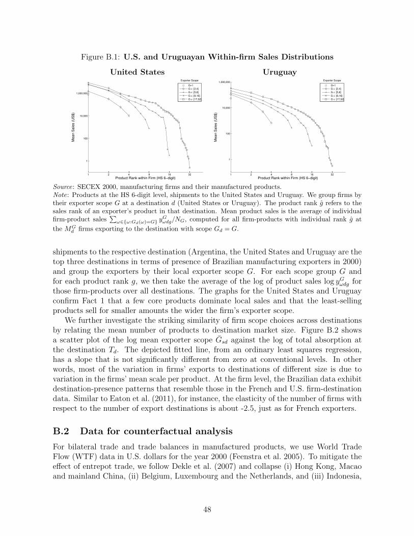
Figure B.1: U.S. and Uruguayan Within-firm Sales Distributions
United States Uruguay
1 2 4 8 16 32
1
100
10,000
1,000,000
Product Rank within Firm (HS 6−digit)
Mean S
ale
s (
US
$)
G=1
G ∈ [2,4]
G ∈ [5,8]
G ∈ [9,16]
G ∈ [17,32]
Exporter Scope
1 2 4 8 16 32
1
100
10,000
1,000,000
Product Rank within Firm (HS 6−digit)
Mean S
ale
s (
US
$)
G=1
G ∈ [2,4]
G ∈ [5,8]
G ∈ [9,16]
G ∈ [17,32]
Exporter Scope
Source: SECEX 2000, manufacturing firms and their manufactured products.Note: Products at the HS 6-digit level, shipments to the United States and Uruguay. We group firms bytheir exporter scope G at a destination d (United States or Uruguay). The product rank g refers to thesales rank of an exporter’s product in that destination. Mean product sales is the average of individualfirm-product sales
∑ω∈ω:Gd(ω)=G y
Gωdg/NG, computed for all firm-products with individual rank g at
the MGd firms exporting to the destination with scope Gd = G.
shipments to the respective destination (Argentina, the United States and Uruguay are thetop three destinations in terms of presence of Brazilian manufacturing exporters in 2000)and group the exporters by their local exporter scope G. For each scope group G andfor each product rank g, we then take the average of the log of product sales log yGωdg forthose firm-products over all destinations. The graphs for the United States and Uruguayconfirm Fact 1 that a few core products dominate local sales and that the least-sellingproducts sell for smaller amounts the wider the firm’s exporter scope.
We further investigate the striking similarity of firm scope choices across destinationsby relating the mean number of products to destination market size. Figure B.2 showsa scatter plot of the log mean exporter scope Gsd against the log of total absorption atthe destination Td. The depicted fitted line, from an ordinary least squares regression,has a slope that is not significantly different from zero at conventional levels. In otherwords, most of the variation in firms’ exports to destinations of different size is due tovariation in the firms’ mean scale per product. At the firm level, the Brazilian data exhibitdestination-presence patterns that resemble those in the French and U.S. firm-destinationdata. Similar to Eaton et al. (2011), for instance, the elasticity of the number of firms withrespect to the number of export destinations is about -2.5, just as for French exporters.
B.2 Data for counterfactual analysis
For bilateral trade and trade balances in manufactured products, we use World TradeFlow (WTF) data in U.S. dollars for the year 2000 (Feenstra et al. 2005). To mitigate theeffect of entrepot trade, we follow Dekle et al. (2007) and collapse (i) Hong Kong, Macaoand mainland China, (ii) Belgium, Luxembourg and the Netherlands, and (iii) Indonesia,
48
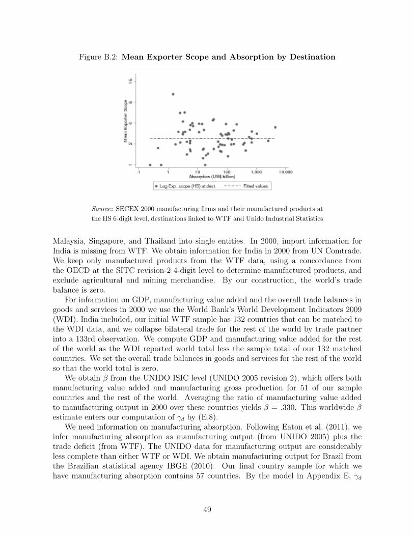
Figure B.2: Mean Exporter Scope and Absorption by Destination
Source: SECEX 2000 manufacturing firms and their manufactured products at
the HS 6-digit level, destinations linked to WTF and Unido Industrial Statistics
Malaysia, Singapore, and Thailand into single entities. In 2000, import information forIndia is missing from WTF. We obtain information for India in 2000 from UN Comtrade.We keep only manufactured products from the WTF data, using a concordance fromthe OECD at the SITC revision-2 4-digit level to determine manufactured products, andexclude agricultural and mining merchandise. By our construction, the world’s tradebalance is zero.
For information on GDP, manufacturing value added and the overall trade balances ingoods and services in 2000 we use the World Bank’s World Development Indicators 2009(WDI). India included, our initial WTF sample has 132 countries that can be matched tothe WDI data, and we collapse bilateral trade for the rest of the world by trade partnerinto a 133rd observation. We compute GDP and manufacturing value added for the restof the world as the WDI reported world total less the sample total of our 132 matchedcountries. We set the overall trade balances in goods and services for the rest of the worldso that the world total is zero.
We obtain β from the UNIDO ISIC level (UNIDO 2005 revision 2), which offers bothmanufacturing value added and manufacturing gross production for 51 of our samplecountries and the rest of the world. Averaging the ratio of manufacturing value addedto manufacturing output in 2000 over these countries yields β = .330. This worldwide βestimate enters our computation of γd by (E.8).
We need information on manufacturing absorption. Following Eaton et al. (2011), weinfer manufacturing absorption as manufacturing output (from UNIDO 2005) plus thetrade deficit (from WTF). The UNIDO data for manufacturing output are considerablyless complete than either WTF or WDI. We obtain manufacturing output for Brazil fromthe Brazilian statistical agency IBGE (2010). Our final country sample for which wehave manufacturing absorption contains 57 countries. By the model in Appendix E, γd
49

is given by (E.8). We use our WTF-WDI-UNIDO data to calculate γd for 57 countries.For the rest of the world, we set γd to the average of our sample (γ = .244) and back outmanufacturing absorption from (E.8).
C Nested Utility
We can generalize the model to consumer preferences N∑k=1
∫ω∈Ωkd
Gkd(ω)∑g=1
ξkdg(ω)1εxkdg(ω)
ε−1ε
εε−1
σ−1σ
dω
σσ−1
where ε > 1, σ > 1, ε 6= σ.
In this case we redefine the product efficiency index and the combined incrementalscope costs as:
H(Gsd) ≡
Gsd(ω)∑g=1
h(g)−(ε−1)
− 1ε−1
and zsd(Gsd, cd) ≡cd fsd(Gsd)
H(Gsd)−(σ−1) −H(Gsd−1)−(σ−1).
(C.4)With these new definitions, the expressions for firm product sales (12) and for aggregatebilateral trade (18) in Lemma 1 remain unaltered. For remaining details on the generalizedmodel see our Online Supplement.
Under this generalization, a firm’s individual products can be less substitutable amongthemselves than with outside products (if ε < σ) or more substitutable (ε > σ). In thelatter case, a firm’s additional products cannibalize sales of its infra-marginal products.The cannibalization effect is symmetric for all products, so relative sales of a firm’s existingproducts are not affected by the introduction of additional products. This constancy ofrelative sales in our model does not carry over to models with CES-preferences and acountable number of firms such as Feenstra and Ma (2008) or to models with non-CESpreferences such as Mayer et al. (2014) and Dhingra (2013).
D Simulation Algorithm and Moments
D.1 Simulation algorithm
Given a candidate estimate Θ, we simulate the export behavior for J sim = 1, 000, 000hypothetical Brazilian firms ω = 1, . . . , J sim shipping to destinations d = 1, ..., N usingour model (N is the observed number of destinations). In order to maintain the stochasticcomponents unchanged as we search over Θ, prior to the simulation routine we draw(i) J sim independent realizations of the firm’s productivity percentile (φω/φ
∗) from thestandard uniform distribution, (ii) J sim × N independent realizations of the firm-specificmarket access costs cωd from the standard log normal distribution, and (iii) J sim×N × Gindependent realizations of individual product appeal shocks ξωdg from the standard log
50
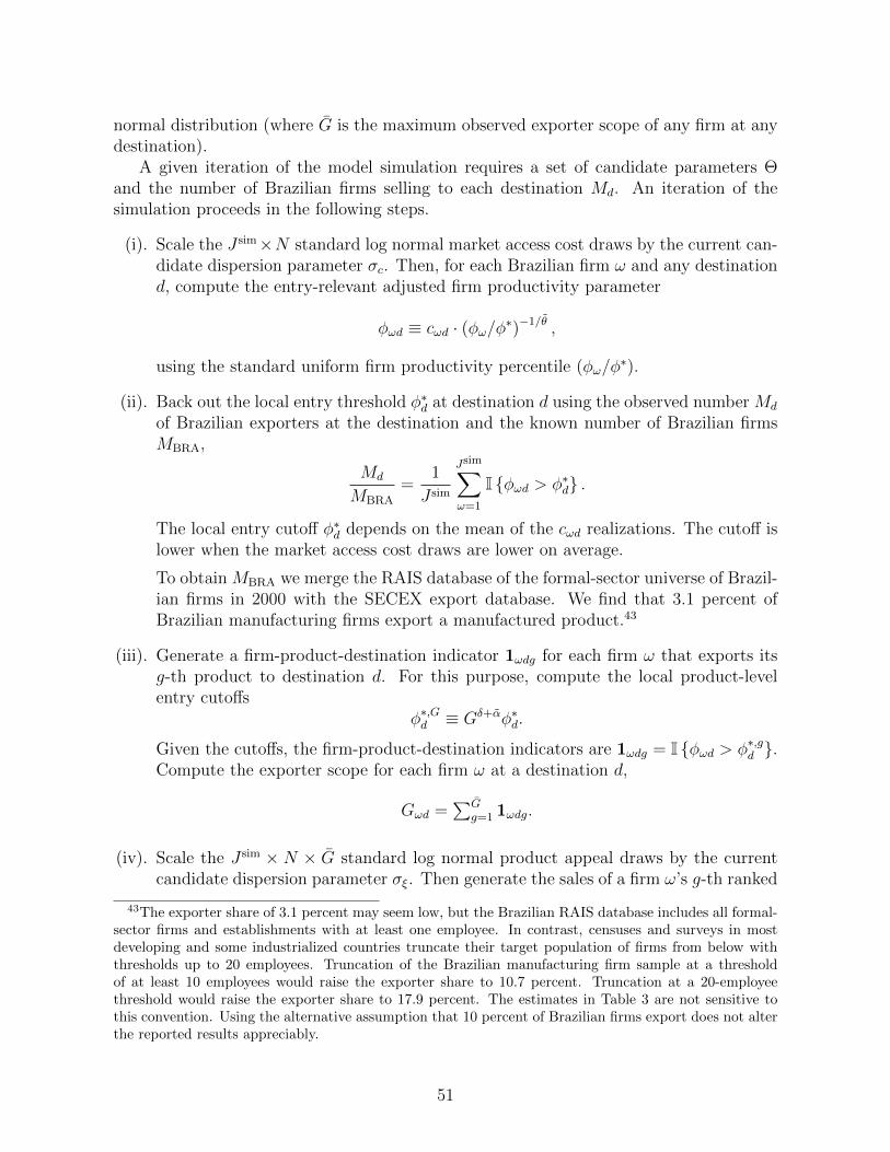
normal distribution (where G is the maximum observed exporter scope of any firm at anydestination).
A given iteration of the model simulation requires a set of candidate parameters Θand the number of Brazilian firms selling to each destination Md. An iteration of thesimulation proceeds in the following steps.
(i). Scale the J sim×N standard log normal market access cost draws by the current can-didate dispersion parameter σc. Then, for each Brazilian firm ω and any destinationd, compute the entry-relevant adjusted firm productivity parameter
φωd ≡ cωd · (φω/φ∗)−1/θ ,
using the standard uniform firm productivity percentile (φω/φ∗).
(ii). Back out the local entry threshold φ∗d at destination d using the observed number Md
of Brazilian exporters at the destination and the known number of Brazilian firmsMBRA,
Md
MBRA
=1
J sim
Jsim∑ω=1
I φωd > φ∗d .
The local entry cutoff φ∗d depends on the mean of the cωd realizations. The cutoff islower when the market access cost draws are lower on average.
To obtain MBRA we merge the RAIS database of the formal-sector universe of Brazil-ian firms in 2000 with the SECEX export database. We find that 3.1 percent ofBrazilian manufacturing firms export a manufactured product.43
(iii). Generate a firm-product-destination indicator 1ωdg for each firm ω that exports itsg-th product to destination d. For this purpose, compute the local product-levelentry cutoffs
φ∗,Gd ≡ Gδ+αφ∗d.
Given the cutoffs, the firm-product-destination indicators are 1ωdg = I φωd > φ∗,gd .Compute the exporter scope for each firm ω at a destination d,
Gωd =∑G
g=1 1ωdg.
(iv). Scale the J sim × N × G standard log normal product appeal draws by the currentcandidate dispersion parameter σξ. Then generate the sales of a firm ω’s g-th ranked
43The exporter share of 3.1 percent may seem low, but the Brazilian RAIS database includes all formal-sector firms and establishments with at least one employee. In contrast, censuses and surveys in mostdeveloping and some industrialized countries truncate their target population of firms from below withthresholds up to 20 employees. Truncation of the Brazilian manufacturing firm sample at a thresholdof at least 10 employees would raise the exporter share to 10.7 percent. Truncation at a 20-employeethreshold would raise the exporter share to 17.9 percent. The estimates in Table 3 are not sensitive tothis convention. Using the alternative assumption that 10 percent of Brazilian firms export does not alterthe reported results appreciably.
51
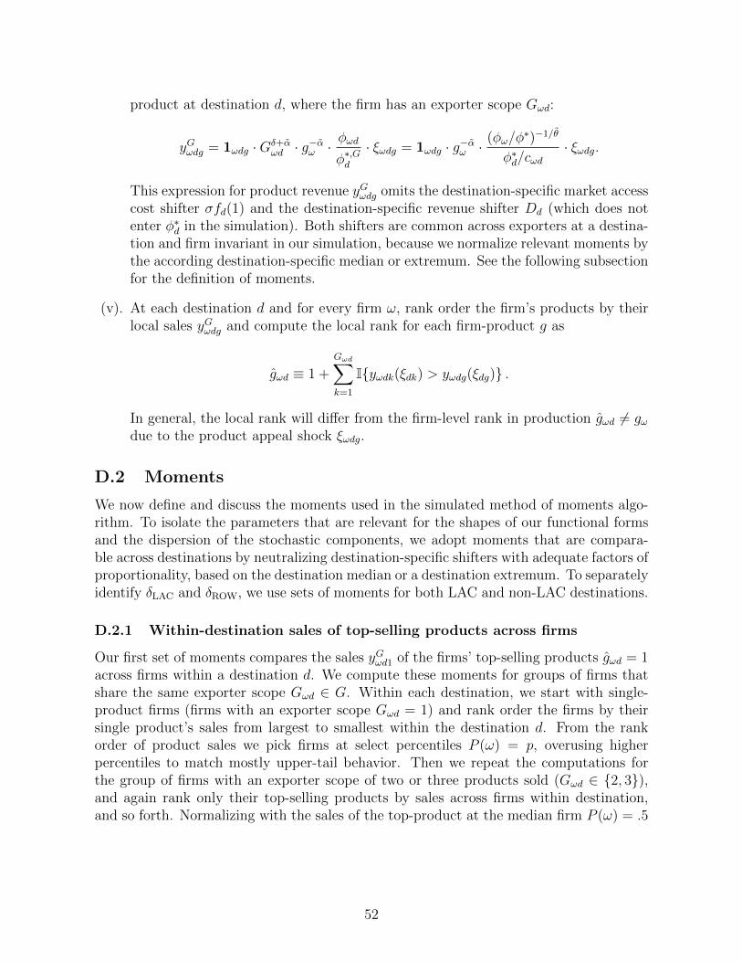
product at destination d, where the firm has an exporter scope Gωd:
yGωdg = 1ωdg ·Gδ+αωd · g
−αω ·
φωd
φ∗,Gd· ξωdg = 1ωdg · g−αω ·
(φω/φ∗)−1/θ
φ∗d/cωd· ξωdg.
This expression for product revenue yGωdg omits the destination-specific market accesscost shifter σfd(1) and the destination-specific revenue shifter Dd (which does notenter φ∗d in the simulation). Both shifters are common across exporters at a destina-tion and firm invariant in our simulation, because we normalize relevant moments bythe according destination-specific median or extremum. See the following subsectionfor the definition of moments.
(v). At each destination d and for every firm ω, rank order the firm’s products by theirlocal sales yGωdg and compute the local rank for each firm-product g as
gωd ≡ 1 +
Gωd∑k=1
Iyωdk(ξdk) > yωdg(ξdg) .
In general, the local rank will differ from the firm-level rank in production gωd 6= gωdue to the product appeal shock ξωdg.
D.2 Moments
We now define and discuss the moments used in the simulated method of moments algo-rithm. To isolate the parameters that are relevant for the shapes of our functional formsand the dispersion of the stochastic components, we adopt moments that are compara-ble across destinations by neutralizing destination-specific shifters with adequate factors ofproportionality, based on the destination median or a destination extremum. To separatelyidentify δLAC and δROW, we use sets of moments for both LAC and non-LAC destinations.
D.2.1 Within-destination sales of top-selling products across firms
Our first set of moments compares the sales yGωd1 of the firms’ top-selling products gωd = 1across firms within a destination d. We compute these moments for groups of firms thatshare the same exporter scope Gωd ∈ G. Within each destination, we start with single-product firms (firms with an exporter scope Gωd = 1) and rank order the firms by theirsingle product’s sales from largest to smallest within the destination d. From the rankorder of product sales we pick firms at select percentiles P (ω) = p, overusing higherpercentiles to match mostly upper-tail behavior. Then we repeat the computations forthe group of firms with an exporter scope of two or three products sold (Gωd ∈ 2, 3),and again rank only their top-selling products by sales across firms within destination,and so forth. Normalizing with the sales of the top-product at the median firm P (ω) = .5
52
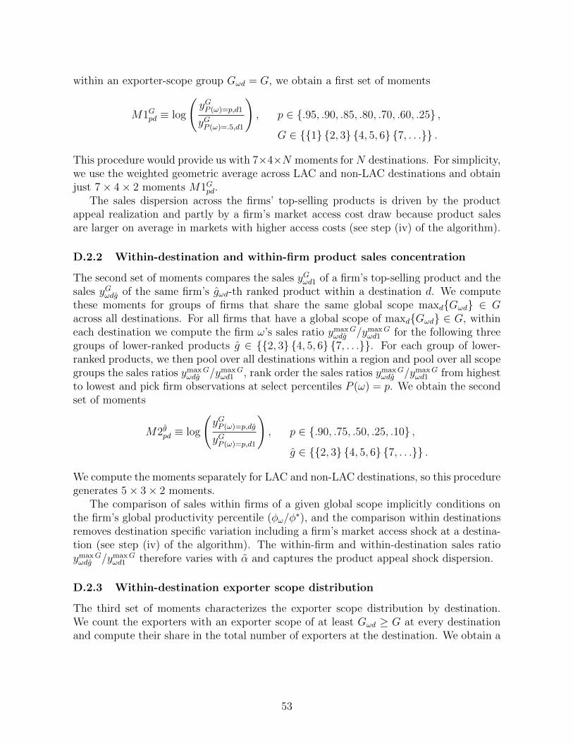
within an exporter-scope group Gωd = G, we obtain a first set of moments
M1Gpd ≡ log
(yGP (ω)=p,d1
yGP (ω)=.5,d1
), p ∈ .95, .90, .85, .80, .70, .60, .25 ,
G ∈ 1 2, 3 4, 5, 6 7, . . . .
This procedure would provide us with 7×4×N moments for N destinations. For simplicity,we use the weighted geometric average across LAC and non-LAC destinations and obtainjust 7× 4× 2 moments M1Gpd.
The sales dispersion across the firms’ top-selling products is driven by the productappeal realization and partly by a firm’s market access cost draw because product salesare larger on average in markets with higher access costs (see step (iv) of the algorithm).
D.2.2 Within-destination and within-firm product sales concentration
The second set of moments compares the sales yGωd1 of a firm’s top-selling product and thesales yGωdg of the same firm’s gωd-th ranked product within a destination d. We computethese moments for groups of firms that share the same global scope maxdGωd ∈ Gacross all destinations. For all firms that have a global scope of maxdGωd ∈ G, withineach destination we compute the firm ω’s sales ratio ymaxG
ωdg /ymaxGωd1 for the following three
groups of lower-ranked products g ∈ 2, 3 4, 5, 6 7, . . .. For each group of lower-ranked products, we then pool over all destinations within a region and pool over all scopegroups the sales ratios ymaxG
ωdg /ymaxGωd1 , rank order the sales ratios ymaxG
ωdg /ymaxGωd1 from highest
to lowest and pick firm observations at select percentiles P (ω) = p. We obtain the secondset of moments
M2gpd ≡ log
(yGP (ω)=p,dg
yGP (ω)=p,d1
), p ∈ .90, .75, .50, .25, .10 ,
g ∈ 2, 3 4, 5, 6 7, . . . .
We compute the moments separately for LAC and non-LAC destinations, so this proceduregenerates 5× 3× 2 moments.
The comparison of sales within firms of a given global scope implicitly conditions onthe firm’s global productivity percentile (φω/φ
∗), and the comparison within destinationsremoves destination specific variation including a firm’s market access shock at a destina-tion (see step (iv) of the algorithm). The within-firm and within-destination sales ratioymaxGωdg /ymaxG
ωd1 therefore varies with α and captures the product appeal shock dispersion.
D.2.3 Within-destination exporter scope distribution
The third set of moments characterizes the exporter scope distribution by destination.We count the exporters with an exporter scope of at least Gωd ≥ G at every destinationand compute their share in the total number of exporters at the destination. We obtain a
53
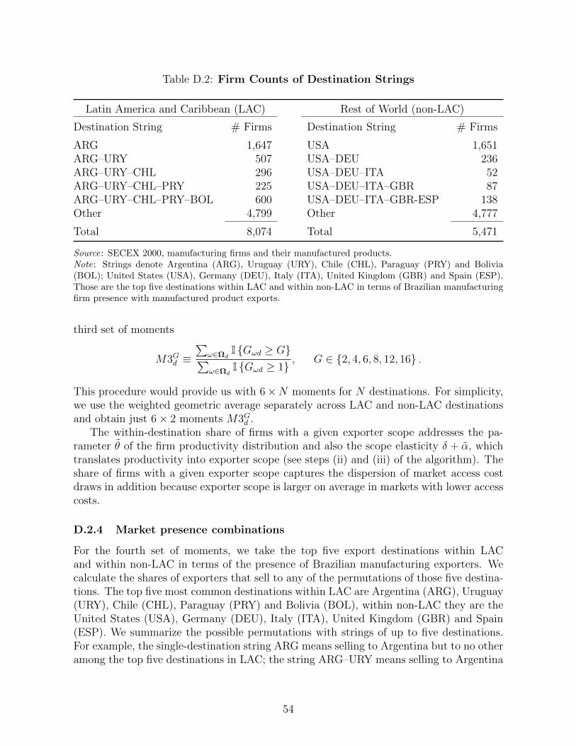
Table D.2: Firm Counts of Destination Strings
Latin America and Caribbean (LAC) Rest of World (non-LAC)
Destination String # Firms Destination String # Firms
ARG 1,647 USA 1,651ARG–URY 507 USA–DEU 236ARG–URY–CHL 296 USA–DEU–ITA 52ARG–URY–CHL–PRY 225 USA–DEU–ITA–GBR 87ARG–URY–CHL–PRY–BOL 600 USA–DEU–ITA–GBR-ESP 138Other 4,799 Other 4,777
Total 8,074 Total 5,471
Source: SECEX 2000, manufacturing firms and their manufactured products.Note: Strings denote Argentina (ARG), Uruguay (URY), Chile (CHL), Paraguay (PRY) and Bolivia(BOL); United States (USA), Germany (DEU), Italy (ITA), United Kingdom (GBR) and Spain (ESP).Those are the top five destinations within LAC and within non-LAC in terms of Brazilian manufacturingfirm presence with manufactured product exports.
third set of moments
M3Gd ≡∑
ω∈Ωd I Gωd ≥ G∑ω∈Ωd I Gωd ≥ 1
, G ∈ 2, 4, 6, 8, 12, 16 .
This procedure would provide us with 6×N moments for N destinations. For simplicity,we use the weighted geometric average separately across LAC and non-LAC destinationsand obtain just 6× 2 moments M3Gd .
The within-destination share of firms with a given exporter scope addresses the pa-rameter θ of the firm productivity distribution and also the scope elasticity δ + α, whichtranslates productivity into exporter scope (see steps (ii) and (iii) of the algorithm). Theshare of firms with a given exporter scope captures the dispersion of market access costdraws in addition because exporter scope is larger on average in markets with lower accesscosts.
D.2.4 Market presence combinations
For the fourth set of moments, we take the top five export destinations within LACand within non-LAC in terms of the presence of Brazilian manufacturing exporters. Wecalculate the shares of exporters that sell to any of the permutations of those five destina-tions. The top five most common destinations within LAC are Argentina (ARG), Uruguay(URY), Chile (CHL), Paraguay (PRY) and Bolivia (BOL), within non-LAC they are theUnited States (USA), Germany (DEU), Italy (ITA), United Kingdom (GBR) and Spain(ESP). We summarize the possible permutations with strings of up to five destinations.For example, the single-destination string ARG means selling to Argentina but to no otheramong the top five destinations in LAC; the string ARG–URY means selling to Argentina
54
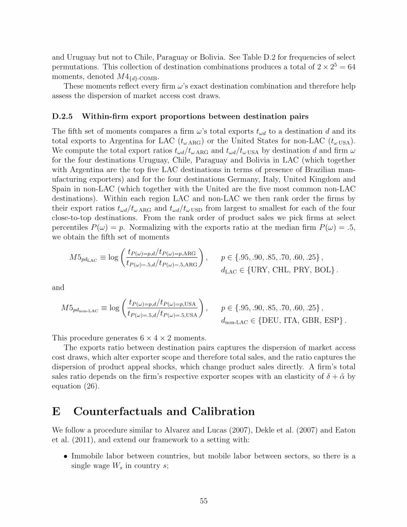
and Uruguay but not to Chile, Paraguay or Bolivia. See Table D.2 for frequencies of selectpermutations. This collection of destination combinations produces a total of 2× 25 = 64moments, denoted M4d-COMB.
These moments reflect every firm ω’s exact destination combination and therefore helpassess the dispersion of market access cost draws.
D.2.5 Within-firm export proportions between destination pairs
The fifth set of moments compares a firm ω’s total exports tωd to a destination d and itstotal exports to Argentina for LAC (tωARG) or the United States for non-LAC (tωUSA).We compute the total export ratios tωd/tωARG and tωd/tωUSA by destination d and firm ωfor the four destinations Uruguay, Chile, Paraguay and Bolivia in LAC (which togetherwith Argentina are the top five LAC destinations in terms of presence of Brazilian man-ufacturing exporters) and for the four destinations Germany, Italy, United Kingdom andSpain in non-LAC (which together with the United are the five most common non-LACdestinations). Within each region LAC and non-LAC we then rank order the firms bytheir export ratios tωd/tωARG and tωd/tωUSD from largest to smallest for each of the fourclose-to-top destinations. From the rank order of product sales we pick firms at selectpercentiles P (ω) = p. Normalizing with the exports ratio at the median firm P (ω) = .5,we obtain the fifth set of moments
M5pdLAC≡ log
(tP (ω)=p,d/tP (ω)=p,ARG
tP (ω)=.5,d/tP (ω)=.5,ARG
), p ∈ .95, .90, .85, .70, .60, .25 ,
dLAC ∈ URY, CHL, PRY, BOL .
and
M5pdnon-LAC≡ log
(tP (ω)=p,d/tP (ω)=p,USA
tP (ω)=.5,d/tP (ω)=.5,USA
), p ∈ .95, .90, .85, .70, .60, .25 ,
dnon-LAC ∈ DEU, ITA, GBR, ESP .
This procedure generates 6× 4× 2 moments.The exports ratio between destination pairs captures the dispersion of market access
cost draws, which alter exporter scope and therefore total sales, and the ratio captures thedispersion of product appeal shocks, which change product sales directly. A firm’s totalsales ratio depends on the firm’s respective exporter scopes with an elasticity of δ + α byequation (26).
E Counterfactuals and Calibration
We follow a procedure similar to Alvarez and Lucas (2007), Dekle et al. (2007) and Eatonet al. (2011), and extend our framework to a setting with:
• Immobile labor between countries, but mobile labor between sectors, so there is asingle wage Ws in country s;
55

• An input bundle that consists of labor and intermediate goods, so such an inputcosts
ws = W βs P
1−βs ;
• A non manufacturing, non-traded final-product sector that only requires labor in-put and produces with a Cobb-Douglas combination of the non-manufacturing andmanufacturing sectors, so final good prices are
P fs = P γ
i W1−γi ;
• Market access costs that require labor at the export destination and are homogeneousof degree 1− θ in foreign wages, so we can rewrite
fsd(1)Fsd = W 1−θd Fsd,
where Fsd denotes mean market access cost costs in terms of labor units;
• Unchanging trade deficits in manufacturing and non-manufacturing sectors;
• Technological parameters and labor endowments that are time invariant.
Using equation (19) for current trade shares λsd, we can express counterfactual tradeshares as
λ′sd =λsd
(W βs P
1−βs
)−θτ−θsd
Fsd∑k λkd
(W βk P
1−βk
)−θτ−θkd
F kd
. (E.5)
The price index (3) can be derived as
P 1−σd =
∑k
∫cd
∫φ∗kd(cd)
Gkd(φ)∑g=1
(σ
wkφ/h(g)
τkd
)1−σ θ (φ∗kd (cd))
θ
φθ+1dφ
dF (cd)
=∑k
(σwkτkd)1−σ Jkb
θkθ
∫cd
∫φ∗kd(cd)
Gkd(φ)∑g=1
h(g)1−σ
φ2−σ+θ
dφ
dF (cd)
=∑k
(σwkτkd)1−σ Jsb
θsθ
1
θ − (σ−1)
(fsd(1)
(φ∗sd)σ−1
)θ−1 ∞∑G=1
fsd(G)−(θ−1)
h(G)θ
∫cd
c−θd dF (cd)
=∑k
(σwkτkd)1−σ Jsb
θsθ
1
θ − (σ−1)
((Pd
στsdws
)σ−1Tdσ
)θ−1
Fkdfkd (1)−θ
κ.The second step uses equation (15). The third step uses Lemma 1 to replace the integralterm. The fourth step uses the log-normal distribution of cd as well as equations (10)
56
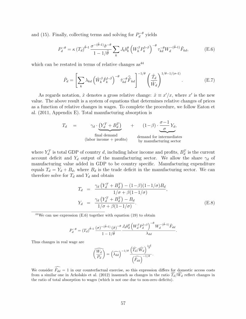
and (15). Finally, collecting terms and solving for P−θd yields
P−θd = κ (Td)θ−1 σ
−(θ−1)σ−θ
1− 1/θ
∑k
Jkbθk
(W βk P
1−βk
)−θτ−θkd W
−(θ−1)d Fkd, (E.6)
which can be restated in terms of relative changes as44
Pd =
[∑k
λkd
(W βk P
1−βk
)−θτ−θkd
F kd
]−1/θ(Td
Wd
)1/θ−1/(σ−1)
. (E.7)
As regards notation, x denotes a gross relative change: x ≡ x′/x, where x′ is the newvalue. The above result is a system of equations that determines relative changes of pricesas a function of relative changes in wages. To complete the procedure, we follow Eaton etal. (2011, Appendix E). Total manufacturing absorption is
Td = γd ·(Y Td +BT
d
)︸ ︷︷ ︸final demand
(labor income + profits)
+ (1−β) · σ−1
σYd︸ ︷︷ ︸,
demand for intermediatesby manufacturing sector
where Y Td is total GDP of country d, including labor income and profits, BT
d is the currentaccount deficit and Yd output of the manufacturing sector. We allow the share γd ofmanufacturing value added in GDP to be country specific. Manufacturing expenditureequals Td = Yd + Bd, where Bd is the trade deficit in the manufacturing sector. We cantherefore solve for Td and Yd and obtain
Td =γd(Y Td +BT
d
)− (1−β)(1−1/σ)Bd
1/σ + β(1−1/σ),
Yd =γd(Y Td +BT
d
)−Bd
1/σ + β(1−1/σ). (E.8)
44We can use expression (E.6) together with equation (19) to obtain
P−θd = (Td)θ−1 (σ)−(θ−1) (σ)
−θ
1− 1/θ
Jdbθd
(W βd P
1−βd
)−θW−(θ−1)d Fdd
λdd.
Thus changes in real wage are (Wd
Pd
)=(λdd
)−1/θ (Td/Wd
) 1−θθ
(Fdd)−1/θ .
We consider Fdd = 1 in our counterfactual exercise, so this expression differs for domestic access costsfrom a similar one in Arkolakis et al. (2012) inasmuch as changes in the ratio Td/Wd reflect changes inthe ratio of total absorption to wages (which is not one due to non-zero deficits).
57

We assume γd is time invariant, so we solve equation (E.8) for γd using 2000 baseline data.To summarize, using the Dekle et al. (2007) algorithm, we can compute how given
relative changes in market access costs F kd lead to λsd, Pd, Wd. Denoting future variableswith a prime, we find T ′d, Y
′d by inspecting equations (E.5), (E.6) and imposing the market
clearing condition
Y ′sLs =N∑k=1
λ′skT′k. (E.9)
58