The exploration of numerical methods and noise modellingtechniques applied to the Trailing Edge Noise case withevaluation of their suitability for aero-acoustic design

Stanislav Proskurov, Sergey Karabasov and Vasily Semiletov

School of Engineering and Materials ScienceQueen Mary University of London

CEAA International Workshop, Svetlogorsk, Russia, September 24-27, 2014

1Queen Mary University of London

Overview

1) Aim of current work

2) Numerical methods

3) Computational cases

4) Results

5) Conclusions

6) Questions

Queen Mary University of London 2

Aim of current work

Test the capability of CAA stochastic Fast Random Particle Mesh (FRPM) method to predict broadband noise on a benchmark test case –trailing edge noise

- Assess the potential of the FRPM method

- Develop the method to overcome current shortcomings…

- Provide design trends in days rather than months

Use high-fidelity ‘state of the art’ LES CFD-CAA to understand the specific noise mechanisms

- How the stochastic FRPM method may be improved?

Queen Mary University of London 3

Numerical methods

FE Discontinuous Galerkin solver

Stochastic source generation

Filtering of a convecting white noise field approach

Requires a steady state RANS

simulation

CABARET-FD based on MILES+FWH

MILES scheme with improved dispersion and dissipation

properties

High-fidelity LES

simulation

Queen Mary University of London 4

Numerical methodsPros & Cons

FE Discontinuous Galerkin solver

Much less expensive!

Requires RANS solution to provide 1 point statistics

Less sensitive to mesh type / refinement / solver numerics

RANS uses physics assumptions (correlations / turbulent energy spectra)

RANS modelling has poor accuracy for predicting flow separation

No tonal noise components

CABARET-FD based on MILES+FWH

Large scale turbulence resolved rather than modelled

Has the greatest potential to provide accurate, physically realistic solution

Best for understanding the nature of acoustic sources for a specific problem

Computationally expensive

Sensitive to mesh type and refinement

Queen Mary University of London 5

FE DG solver

Quadrature Free Discontinuous Galerkin solver (time domain)

Parallel, unstructured

Acoustic Perturbation Equations – 4 (APE−4 variant)�Low dissipation/dispersion ADER� explicit time steppingAcoustic sources obtained via FRPM method2D and 3D parallelised FRPM

1. Ewert, R. and Schroder, W., “Acoustic perturbation equations based on flow decomposition via source filtering,” Journal of Computational Physics, Vol. 188, No. 2, 2003, pp. 365–398.

2. Toro, E. F., Millington, R. C., and Nejad, L. A. M., “Towards Very High-Order Godunov Schemes,” Godunov Methods: Theory and Applications. Edited review, E. F. Toro (Editor), Vol. 3352, 2001, pp. 905–937.

Queen Mary University of London 6

FE DG solver

System of equations of the form:

��(�, ��� ���(�, ���� �(�, �Expand the solution, flux functionsand sources in terms of nodal basis functions, ��(��

� �, � ��(���(��� �, � ��(����(�� �, � ��(���(�Multiplying by the test function, integrating over the volume, applying integration by parts and the divergence theorem yields:

� ���� ���� ��� � ������������ � � ��������� ����� � ����������� � �������

Further, assuming �� is linear (computing Jacobian matrix separately to realise QF concept)

Queen Mary University of London 7

�(� exp!� "4 �2%2 & '( ) 23" +12 ≈ 0.46+12

1(�, � � '� �(� � �′ 3(�′ , �

FRPM method in a nutshell

RANS + � 4 SST Map the mean flow to:Auxiliary cartesian FRPM grid & CAA prism O-grid

Provide…Integral length scale

Turbulent kinetic energy +54 or 6, sound speed,

density, 7 8 9 velocities

1) Seed random particles and

convect them with a mean flow

2) Interpolate the random numbers onto the neighbouring auxiliary mesh nodes

3) Perform the integral at every node

Queen Mary University of London 8

3 – unity white noise field

FRPM method in a nutshellDifferent source models are possible,

‘Source A’: used here:

APE-4 equations could be written out as following,

RHS source term

3. Ewert, R., Dierke, J., Siebert, et al., “CAA broadband noise prediction for aeroacoustic design”, Journal of Sound and

vibration, Vol. 330, 2011, pp. 4139-4160.

Queen Mary University of London 9

7′ ∇ × 1

4′ ∇ × 7′ = �>?@ × A′ B � >?′ × A@B � >(?′ × A′ ′B

?′ ∝ !1 � "�22%2 & exp!� "2 �2

%2 &

�D′�� ���E (F02G07E′ D′70E 0

�7H ′�� ���H !70E 7E′ D′G0& =

Compact Accurately Boundary Adjusting high-Resolution Technique

Properties

Explicit, second order in space & time

Non-dissipative & low dispersive

Conservative form

Compact one cell stencil in space & time

Nonlinear flux correction based on maximum principle

Nonlinear flux reconstruction based on the minimum solution variation

Queen Mary University of London 10

S.A. Karabasov and V.M. Goloviznin. “Compact Accurately Boundary Adjusting high-REsolution Technique for Fluid Dynamics”, J. Comput.Phys., 228(2009), pp. 7426–7451.

Computational Cases

1) CASE#1 BANC WorkshopDG FE – FRPM

2) Experiment of Brooks, Pope and Marcolini (1989)

CABARET – LES

NACA0012, F 0.4, UJ 56 m/s

M = 0.1664, Re= 1.5MK∞ = 281.5K, G = 1.181 +M/O:, P∞ = 95429 Pa, AoA = 0° sharp TE,

untripped

NACA0012, F 0.1524, z = 3F exp.,

z = 0.1F sim.,

M = 0.1150, Re= 408k

AoA = 0° sharp TE,

untripped

Queen Mary University of London 11

Computational Mesh –Case 1

Queen Mary University of London 12

C-grid hexahedron type in 2D incorporating a single element width in spanwise direction

216 mesh points per side of the aerofoil ~80 of 216 on the LE per side (~5% of the chord)

117 mesh points in the far-field (normal direction) Target y+ of 1

Far-field boundaries 25c away from the aerofoilMaximal element expansion ratio~5-10% on the aerofoil surface

68k elements in total per 2D layer up to 30% in the far-field

Computational CasesResources comparison

Case 1

RANS + � 4 SST

68,000cells (2D)

singlecore

10 min.

32cores (4 assigned to FRPM and 28 to CAA)

~24 hours

Case 2

LES

8.2 M cells

2880cores (HECToR)

240 hours

Queen Mary University of London 13

CFD

Mesh

Time(wall clock)

CAA

ResultsNear-field results– Case 1

Inflection point at y ~14-16 mm

Queen Mary University of London 14

U1 U∞⁄

+K U∞2⁄

R,mm

R,mm

Results

Queen Mary University of London 15

TU NASA validation case:

NACA0012, F 1.52, UJ 59 m/sM = 0.17, Re= 5.97MK∞ = 288.16 K, G = 1.225 +M/O:, V = 1.7894 × 10WX, sharp TE

Results

Acoustic results– Case 1

Instantaneous acoustic pressure field

green -DLR 60 m/s, red - our 56 m/s

Queen Mary University of London 16

Results

Near-field results– Case 2

x/c = 0.9

Iso-surfaces of Q-criterion

Queen Mary University of London 17

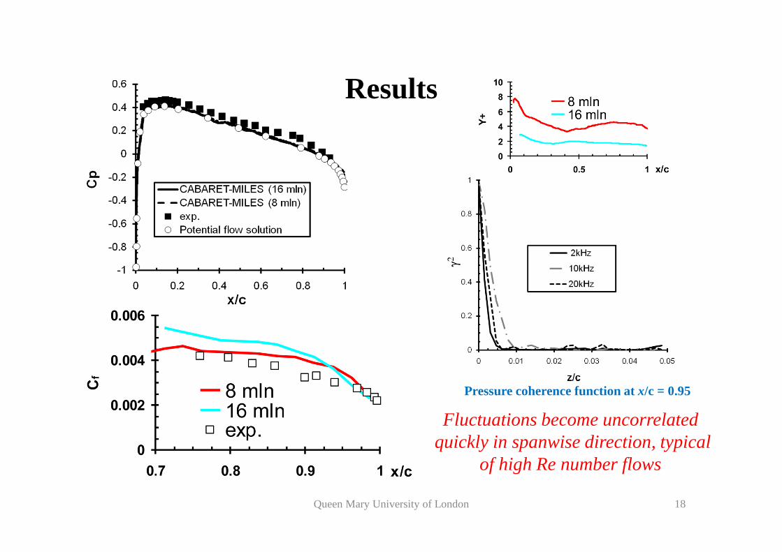
Results

Queen Mary University of London 18

Pressure coherence function at x/c = 0.95

Fluctuations become uncorrelated quickly in spanwise direction, typical

of high Re number flows

Results

Acoustic results– Case 2

Sound pressure level at observer location x = c, y = 8c, z = 0.5c

Queen Mary University of London 19

V.A. Semiletov and S.A. Karabasov, "CABARET scheme for computational aero acoustics: extension to asynchronous time stepping and 3D flow modelling", Int. J. Aeroacoustics, 13 (3-4): 321 – 336, 2014.

ConclusionsFRPM method provides the quick prediction of broadband noise levels that showed the similar trend as experimental results for the trailing edge noise case

FRPM method has a great potential to study design optimisationLES simulation can be used to verify the noise levels of the final design.

Confidence in modelling is gained by using: Two different CFD approachesTwo different acoustic source modelsTwo different acoustic codes & equations

High-fidelity LES may be used to provide realistic correlations / turbulence energy spectra / length scalesto improve the FRPM method

Queen Mary University of London 20

Thank you!

Questions?

Queen Mary University of London 21