The Expected Value - University of Arizonamath.arizona.edu/~jwatkins/H_expectedvalue.pdf · Topic 8 The Expected Value Among the simplest summaries of quantitative data is the sample

Topic 8

The Expected Value

Among the simplest summaries of quantitative data is the sample mean. Given a random variable, the correspondingconcept is given a variety of names, the distributional mean, the expectation or the expected value. We beginwith the case of discrete random variables where this analogy is more apparent. The formula for continuous randomvariables is obtained by approximating with a discrete random variable and noticing that the formula for the expectedvalue is a Riemann sum. Thus, expected values for continuous random variables are determined by computing anintegral.

8.1 Definition and PropertiesRecall for a data set taking numerical values x

1

, x2

, . . . , xn, one of the methods for computing the sample mean of areal-valued function of the data is accomplished by evaluating the sum,

h(x) =X

x

h(x)p(x),

where p(x) is the proportion of observations taking the value x.For a finite sample space ⌦ = {!

1

,!2

, . . . ,!N} and a probability P on ⌦, we can define the expectation or theexpected value of a random variable X by an analogous average,

EX =

NX

j=1

X(!j)P{!j}. (8.1)

More generally for a real-valued function g of the random vector X = (X1

, X2

, . . . , Xn), we have the formula

Eg(X) =

NX

j=1

g(X(!j))P{!j}. (8.2)

Notice that even though we have this analogy, the two formulas come from very different starting points. The valueof h(x) is derived from data whereas no data are involved in computing Eg(X). The starting point for the expectedvalue is a probability model.

Example 8.1. Roll one die. Then ⌦ = {1, 2, 3, 4, 5, 6}. Let X be the value on the die. So, X(!) = !. If the die isfair, then the probability model has P{!} = 1/6 for each outcome !. Using the formula (8.1), the expected value

EX = 1 · P{1}+ 2 · P{2}+ 3 · P{3}+ 4 · P{4}+ 5 · P{5}+ 6 · P{6}

= 1 · 16

+ 2 · 16

+ 3 · 16

+ 4 · 16

+ 5 · 16

+ 6 · 16

=

21

6

=

7

2

.

119

Introduction to the Science of Statistics The Expected Value

An example of an unfair dice would be the probability with P{1} = P{2} = P{3} = 1/4 and P{4} = P{5} =

P{6} = 1/12. In this case, the expected value

EX = 1 · 14

+ 2 · 14

+ 3 · 14

+ 4 · 1

12

+ 5 · 1

12

+ 6 · 1

12

=

11

4

.

Exercise 8.2. Use the formula (8.2) with g(x) = x2 to find EX2 for these two examples.

Two properties of expectation are immediate from the formula for EX in (8.1):

1. If X(!) � 0 for every outcome ! 2 ⌦, then every term in the sum in (8.1) is nonnegative and consequentlytheir sum EX � 0.

2. Let X1

and X2

be two random variables and c1

, c2

be two real numbers, then by using g(x1

, x2

) = c1

x1

+ c2

x2

and the distributive property to the sum in (8.2), we find out that

E[c1

X1

+ c2

X2

] = c1

EX1

+ c2

EX2

.

The first of these properties states that nonnegative random variables have nonnegative expected value. The secondstates that expectation is a linear operation. Taking these two properties together, we say that the operation of takingan expectation

X 7! EX

is a positive linear functional. We have studied extensively another example of a positive linear functional, namely,the definite integral

g 7!Z b

ag(x) dx

that takes a continuous positive function and gives the area between the graph of g and the x-axis between the verticallines x = a and x = b. For this example, these two properties become:

1. If g(x) � 0 for every x 2 [a, b], thenR ba g(x) dx � 0.

2. Let g1

and g2

be two continuous functions and c1

, c2

be two real numbers, thenZ b

a(c

1

g1

(x) + c2

g2

(x)) dx = c1

Z b

ag1

(x) dx+ c2

Z b

ag2

(x) dx.

This analogy will be useful to keep in mind when considering the properties of expectation.

Example 8.3. If X1

and X2

are the values on two rolls of a fair die, then the expected value of the sum

E[X1

+X2

] = EX1

+ EX2

=

7

2

+

7

2

= 7.

8.2 Discrete Random VariablesBecause sample spaces can be extraordinarily large even in routine situations, we rarely use the probability space ⌦

as the basis to compute the expected value. We illustrate this with the example of tossing a coin three times. Let Xdenote the number of heads. To compute the expected value EX , we can proceed as described in (8.1). For the tablebelow, we have grouped the outcomes ! that have a common value x = 3, 2, 1 or 0 for X(!).

From the definition of expectation in (8.1), EX , the expected value of X is the sum of the values in column F. Wewant to now show that EX is also the sum of the values in column G.

Note, for example, that, three outcomes HHT,HTH and THH each give a value of 2 for X . Because theseoutcomes are disjoint, we can add probabilities

P{HHT}+ P{HTH}+ P{THH} = P{HHT,HTH, THH}

120


A B C D E F G! X(!) x P{!} P{X = x} X(!)P{!} xP{X = x}

HHH 3 3 P{HHH} P{X = 3} X(HHH)P{HHH} 3P{X = 3}HHT 2 P{HHT} X(HHT )P{HHT}HTH 2 2 P{HTH} P{X = 2} X(HTH)P{HTH} 2P{X = 2}THH 2 P{THH} X(THH)P{THH}HTT 1 P{HTT} X(HHT )P{HHT}TTH 1 1 P{THT} P{X = 1} X(HTH)P{HTH} 1P{X = 1}THT 1 P{TTH} X(THH)P{THH}TTT 0 0 P{TTT} P{X = 0} X(TTT )P{TTT} 0P{X = 0}

Table I: Developing the formula for EX for the case of the coin tosses.

But, the event

{HHT,HTH, THH} can also be written as the event {X = 2}.

This is shown for each value of x in column C, P{X = x}, the probabilities in column E are obtained as a sum ofprobabilities in column D.

Thus, by combining outcomes that result in the same value for the random variable, the sums in the boxes incolumn F are equal to the value in the corresponding box in column G. and thus their total sums are the same. In otherwords,

EX = 0 · P{X = 0}+ 1 · P{X = 1}+ 2 · P{X = 2}+ 3 · P{X = 3}.

As in the discussion above, we can, in general, find Eg(X). First, to build a table, denote the outcomes in theprobability space ⌦ as !

1

, . . . ,!k,!k+1

, . . . ,!N and the state space for the random variable X as x1

, . . . , xi, . . . , xn.Note that we have partitioned the sample space ⌦ into the outcomes ! that result in the same value x for the random

variable X(!). This is shown by the horizontal lines in the table above showing that X(!k) = X(!k+1

) = · · · = xi.The equality of sum of the probabilities in a box in columns D and and the probability in column E can be written

X

!;X(!)=xi

P{!} = P{X = xi}.

A B C D E F G! X(!) x P{!} P{X = x} g(X(!))P{!} g(x)P{X = x}...

......

......

......

!k X(!k) P{!k} g(X(!k))P{!k}!k+1

X(!k+1

) xi P{!k+1

} P{X = xi} g(X(!k+1

))P{!k+1

} g(xi)P{X = xi}...

......

......

......

......

......

Table II: Establishing the identity in (8.3) from (8.2). Arrange the rows of the table so that common values of X(!k

), X(!k+1), . . . in the box

in column B have the value xi

in column C. Thus, the probabilities in a box in column D sum to give the probability in the corresponding box incolumn E. Because the values for g(X(!

k

)), g(X(!k+1)), . . . equal g(x

i

), the sum in a box in column F sums to the value in corresponding boxin column G. Thus, the sums in columns F and G are equal. The sum in column F is the definition in (8.2). The sum in column G is the identity(8.3).

121


For these particular outcomes, g(X(!)) = g(xi) and the sum of the values in a boxes in column F,X

!;X(!)=xi

g(X(!))P{!} =

X

!;X(!)=xi

g(xi)P{!} = g(xi)P{X = xi},

the value in the corresponding box in column G. Now, sum over all possible value for X for each side of this equation.

Eg(X) =

X

!

g(X(!))P{!} =

nX

i=1

g(xi)P{X = xi} =

nX

i=1

g(xi)fX(xi)

where fX(xi) = P{X = xi} is the probability mass function for X .The identity

Eg(X) =

nX

i=1

g(xi)fX(xi) =

X

x

g(x)fX(x) (8.3)

is the most frequently used method for computing the expectation of discrete random variables. We will soon see howthis identity can be used to find the expectation in the case of continuous random variables

Example 8.4. Flip a biased coin twice and let X be the number of heads. Then, to compute the expected value of Xand X2 we construct a table to prepare to use (8.3).

x fX(x) xfX(x) x2fX(x)0 (1� p)2 0 0

1 2p(1� p) 2p(1� p) 2p(1� p)2 p2 2p2 4p2

sum 1 2p 2p+ 2p2

Thus, EX = 2p and EX2

= 2p+ 2p2.

Exercise 8.5. Draw 5 cards from a standard deck. Let X be the number of hearts. Use R to find EX and EX2.

A similar formula to (8.3) holds if we have a vector of random variables X = (X1

, X2

, . . . , Xn), fX , the jointprobability mass function and g a real-valued function of x = (x

1

, x2

, . . . , xn). In the two dimensional case, this takesthe form

Eg(X1

, X2

) =

X

x1

X

x2

g(x1

, x2

)fX1,X2(x1

, x2

). (8.4)

We will return to (8.4) in computing the covariance of two random variables.

8.3 Bernoulli TrialsBernoulli trials are the simplest and among the most common models for an experimental procedure. Each trial hastwo possible outcomes, variously called,

heads-tails, yes-no, up-down, left-right, win-lose, female-male, green-blue, dominant-recessive, or success-failure

depending on the circumstances. We will use the principles of counting and the properties of expectation to analyzeBernoulli trials. From the point of view of statistics, the data have an unknown success parameter p. Thus, the goal ofstatistical inference is to make as precise a statement as possible for the value of p behind the production of the data.Consequently, any experimenter that uses Bernoulli trials as a model ought to mirror its properties closely.

Example 8.6 (Bernoulli trials). Random variables X1

, X2

, . . . , Xn are called a sequence of Bernoulli trials providedthat:

1. Each Xi takes on two values, namely, 0 and 1. We call the value 1 a success and the value 0 a failure.

122


2. Each trial has the same probability for success, i.e., P{Xi = 1} = p for each i.

3. The outcomes on each of the trials is independent.

For each trial i, the expected value

EXi = 0 · P{Xi = 0}+ 1 · P{Xi = 1} = 0 · (1� p) + 1 · p = p

is the same as the success probability. Let Sn = X1

+X2

+ · · ·+Xn be the total number of successes in n Bernoullitrials. Using the linearity of expectation, we see that

ESn = E[X1

+X2

· · ·+Xn] = p+ p+ · · ·+ p = np,

the expected number of successes in n Bernoulli trials is np.

In addition, we can use our ability to count to determine the probability mass function for Sn. Beginning with aconcrete example, let n = 8, and the outcome

success, fail, fail, success, fail, fail, success, fail.

Using the independence of the trials, we can compute the probability of this outcome:

p⇥ (1� p)⇥ (1� p)⇥ p⇥ (1� p)⇥ (1� p)⇥ p⇥ (1� p) = p3(1� p)5.

Moreover, any of the possible�

8

3

�

particular sequences of 8 Bernoulli trials having 3 successes also has probabilityp3(1 � p)5. Each of the outcomes are mutually exclusive, and, taken together, their union is the event {S

8

= 3}.Consequently, by the axioms of probability, we find that

P{S8

= 3} =

✓

8

3

◆

p3(1� p)5.

Returning to the general case, we replace 8 by n and 3 by x to see that any particular sequence of n Bernoullitrials having x successes has probability

px(1� p)n�x.

In addition, we know that we have✓

n

x

◆

mutually exclusive sequences of n Bernoulli trials that have x successes. Thus, we have the mass function

fSn

(x) = P{Sn = x} =

✓

n

x

◆

px(1� p)n�x, x = 0, 1, . . . , n.

The fact that the sumnX

x=0

fSn

(x) =nX

x=0

✓

n

x

◆

px(1� p)n�x= (p+ (1� p))n = 1

n= 1

follows from the binomial theorem. Consequently, Sn is called a binomial random variable.

In the exercise above where X is the number of hearts in 5 cards, let Xi = 1 if the i-th card is a heart and 0 if itis not a heart. Then, the Xi are not Bernoulli trials because the chance of obtaining a heart on one card depends onwhether or not a heart was obtained on other cards. Still,

X = X1

+X2

+X3

+X4

+X5

is the number of hearts and

EX = EX1

+ EX2

+ EX3

+ EX4

+ EX5

= 1/4 + 1/4 + 1/4 + 1/4 + 1/4 = 5/4.

123


8.4 Continuous Random Variables

!0.5 !0.25 0 0.25 0.5 0.75 1 1.25 1.5 1.75 2

0

0.5

1

1.5

2

2.5

3

density fX

round down

! x

Figure 8.1: The discrete random variable ˜X is obtained by rounding down thecontinuous random variable X to the nearest multiple of �x. The mass functionfX

(x) is the integral of the density function from x to x + �x indicated at thearea under the density function between two consecutive vertical lines.

For X a continuous random variable with densityfX , consider the discrete random variable ˜X ob-tained from X by rounding down. Say, for exam-ple, we give lengths by rounding down to the near-est millimeter. Thus, ˜X = 2.134 meters for anylengths X satisfying 2.134 meters < X 2.135meters.

The random variable ˜X is discrete. To be pre-cise about the rounding down procedure, let �x bethe spacing between values for ˜X . Then, x, an inte-ger multiple of �x, represents a possible value for˜X , then this rounding becomes

˜X = x if and only if x < X x+�x.

With this, we can give the mass function

f˜X(x) = P{ ˜X = x} = P{x < X x+�x}.

Now, by the property of the density function,

P{x X < x+�x} ⇡ fX(x)�x. (8.5)

In this case, we need to be aware of a possible source of confusion due to the similarity in the notation that we have forboth the mass function f

˜X for the discrete random variable ˜X and a density function fX for the continuous randomvariable X .

For this discrete random variable ˜X , we can use identity (8.3) and the approximation in (8.5) to approximate theexpected value.

Eg( ˜X) =

X

x

g(x)f˜X(x) =

X

x

g(x)P{x X < x+�x}

⇡X

x

g(x)fx(x)�x.

This last sum is a Riemann sum and so taking limits as �x ! 0, we have that ˜X converges to X and the Riemannsum converges to the definite integral. Thus,

Eg(X) =

Z 1

�1g(x)fX(x) dx. (8.6)

As in the case of discrete random variables, a similar formula to (8.6) holds if we have a vector of random variablesX = (X

1

, X2

, . . . , Xn), fX , the joint probability density function and g a real-valued function of the vector x =

(x1

, x2

, . . . , xn). The expectation in this case is an n-dimensional Riemann integral. For example, if X1

and X2

hasjoint density fX1,X2(x1

, x2

), then

Eg(X1

, X2

) =

Z 1

�1

Z 1

�1g(x

1

, x2

)fX1,X2(x1

, x2

) dx2

dx1

provided that the improper Riemann integral converges.

Example 8.7. For the dart example, the density fX(x) = 2x on the interval [0, 1] and 0 otherwise. Thus,

EX =

Z

1

0

x · 2x dx =

Z

1

0

2x2 dx =

2

3

x3

�

�

�

1

0

=

2

3

.

124


0.0 0.5 1.0 1.5

0.0

0.2

0.4

0.6

0.8

1.0

Cumulative Distribution Function

x

0.0 0.5 1.0 1.5

0.0

0.2

0.4

0.6

0.8

1.0

0.0 0.5 1.0 1.5

0.0

0.2

0.4

0.6

0.8

1.0

Survival Function

x

0.0 0.5 1.0 1.5

0.0

0.2

0.4

0.6

0.8

1.0

Figure 8.2: The cumulative distribution function FX

(x) and the survival function ¯FX

(x) = 1 � FX

(x) for the dart board example. Using theexpression (8.7), we see that the expected value EX = 2/3 is the area under the survival function.

Exercise 8.8. If X is a nonnegative random variable, then FX(0) = 0.

If we were to compute the mean of T , an exponential random variable,

ET =

Z 1

0

tfT (t) dt =

Z 1

0

t�e��t dt,

then our first step is to integrate by parts. This situation occurs with enough regularity that we will benefit in makingthe effort to see how integration by parts gives an alternative to computing expectation. In the end, we will see ananalogy between the mean with the survival function P{X > x} = 1�FX(x) = ¯FX(x), and the sample mean withthe empirical survival function.

Let X be a positive random variable, then the expectation is the improper integral

EX =

Z 1

0

xfX(x) dx

(The unusual choice for v is made to simplify some computations and to anticipate the appearance of the survivalfunction.)

u(x) = x v(x) = �(1� FX(x)) = � ¯FX(x)u0(x) = 1 v0(x) = fX(x) = � ¯F 0

X(x).

First integrate from 0 to b and take the limit as b ! 1. Then, because FX(0) = 0, ¯FX(0) = 1 and

Z b

0

xfX(x) dx = �x ¯FX(x)�

�

�

b

0

+

Z b

0

¯FX(x) dx

= �b ¯FX(b) +

Z b

0

¯FX(x) dx

125


The product term in the integration by parts formula converges to 0 as b ! 1. Thus, we can take a limit to obtainthe identity,

EX =

Z 1

0

P{X > x} dx. (8.7)

Exercise 8.9. Show that the product term in the integration by parts formula does indeed converge to 0 as b ! 1.

In words, the expected value is the area between the cumulative distribution function and the line y = 1 or the areaunder the survival function. For the case of the dart board, we see that the area under the distribution function betweeny = 0 and y = 1 is

R

1

0

x2dx = 1/3, so the area below the survival function EX = 2/3. (See Figure 8.2.)

Example 8.10. Let T be an exponential random variable, then for some �, the survival function ¯FT (t) = P{T >t} = exp(��t). Thus,

ET =

Z 1

0

P{T > t} dt =Z 1

0

exp(��t) dt = � 1

�exp(��t)

�

�

�

1

0

= 0� (� 1

�) =

1

�.

Exercise 8.11. Generalize the identity (8.7) above to X be a positive random variable and g a non-decreasing functionto show that the expectation

Eg(X) =

Z 1

0

g(x)fX(x) dx = g(0) +

Z 1

0

g0(x)P{X > x} dx.

-3 -2 -1 0 1 2 3

0.0

0.1

0.2

0.3

0.4

x

dnorm(x)

Figure 8.3: The density of a standard normal density, drawn in Rusing the command curve(dnorm(x),-3,3).

The most important density function we shall encounter is

�(z) =1p2⇡

exp(�z2

2

), z 2 R.

for Z, the standard normal random variable. Because the func-tion � has no simple antiderivative, we must use a numericalapproximation to compute the cumulative distribution func-tion, denoted � for a standard normal random variable.

Exercise 8.12. Show that � is increasing for z < 0 and de-creasing for z > 0. In addition, show that � is concave downfor z between �1 and 1 and concave up otherwise.

Example 8.13. The expectation of a standard normal randomvariable,

EZ =

1p2⇡

Z 1

�1z exp(�z2

2

) dz = 0

because the integrand is an odd function. Next to evaluate

EZ2

=

1p2⇡

Z 1

�1z2 exp(�z2

2

) dz,

we integrate by parts. (Note the choices of u and v0.)

u(z) = z v(z) = � exp(� z2

2

)

u0(z) = 1 v0(z) = z exp(� z2

2

)

Thus,

EZ2

=

1p2⇡

✓

�z exp(�z2

2

)

�

�

�

1

�1+

Z 1

�1exp(�z2

2

) dz

◆

= 1.

Use l’Hopital’s rule to see that the first term is 0. The fact that the integral of a probability density function is 1 showsthat the second term equals 1.

Exercise 8.14. For Z a standard normal random variable, show that EZ3

= 0 and EZ4

= 3.

126


Histogram of morley[, 3]

morley[, 3]

Frequency

600 700 800 900 1000 1100

05

10

15

20

25

30

-2 -1 0 1 2

700

800

900

1000

Normal Q-Q Plot

Theoretical Quantiles

Sa

mp

le Q

ua

ntile

s

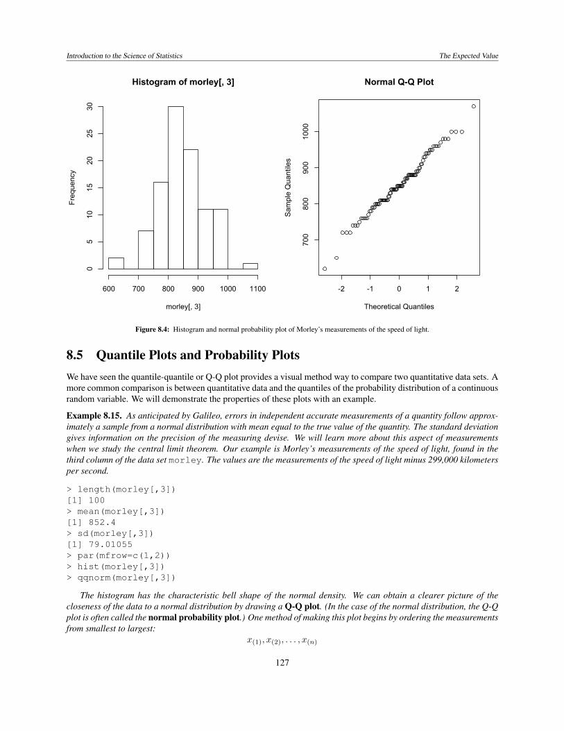
Figure 8.4: Histogram and normal probability plot of Morley’s measurements of the speed of light.

8.5 Quantile Plots and Probability PlotsWe have seen the quantile-quantile or Q-Q plot provides a visual method way to compare two quantitative data sets. Amore common comparison is between quantitative data and the quantiles of the probability distribution of a continuousrandom variable. We will demonstrate the properties of these plots with an example.

Example 8.15. As anticipated by Galileo, errors in independent accurate measurements of a quantity follow approx-imately a sample from a normal distribution with mean equal to the true value of the quantity. The standard deviationgives information on the precision of the measuring devise. We will learn more about this aspect of measurementswhen we study the central limit theorem. Our example is Morley’s measurements of the speed of light, found in thethird column of the data set morley. The values are the measurements of the speed of light minus 299,000 kilometersper second.

> length(morley[,3])[1] 100> mean(morley[,3])[1] 852.4> sd(morley[,3])[1] 79.01055> par(mfrow=c(1,2))> hist(morley[,3])> qqnorm(morley[,3])

The histogram has the characteristic bell shape of the normal density. We can obtain a clearer picture of thecloseness of the data to a normal distribution by drawing a Q-Q plot. (In the case of the normal distribution, the Q-Qplot is often called the normal probability plot.) One method of making this plot begins by ordering the measurementsfrom smallest to largest:

x(1)

, x(2)

, . . . , x(n)

127


If these are independent measurements from a normal distribution, then these values should be close to the quantilesof the evenly space values

1

n+ 1

,2

n+ 1

, · · · , n

n+ 1

(For the Morley data, n = 100). Thus, the next step is to find the values in the standard normal distribution that havethese quantiles. We can find these values by applying �

�1, the inverse distribution function for the standard normal(qnorm in R), applied to the n values listed above. Then the Q-Q plot is the scatterplot of the pairs

✓

x(1)

,��1

✓

1

n+ 1

◆◆

,

✓

x(2)

,��1

✓

2

n+ 1

◆◆

, . . . ,

✓

x(n),�

�1

✓

n

n+ 1

◆◆

Then a good fit of the data and a normal distribution can be seen in how well the plot follows a straight line. Sucha plot can be seen in Figure 8.4.

Exercise 8.16. Describe the normal probability plot in the case in which the data X are skewed right.

8.6 Summary

distribution functionFX(x) = P{X x}

discrete random variable continuous

mass function density functionfX(x) = P{X = x} fX(x)�x ⇡ P{x X < x+�x}

fX(x) � 0 properties fX(x) � 0

P

all x fX(x) = 1

R1�1 fX(x) dx = 1

P{X 2 A} =

P

x2A fX(x) probability P{X 2 A} =

R

AfX(x) dx

Eg(X) =

P

all x g(x)fX(x) expectation Eg(X) =

R1�1 g(x)fX(x) dx

8.7 Names for Eg(X).Several choice for g have special names. We shall later have need for several of these expectations. Others are includedto create a comprehensive reference list.

1. If g(x) = x, then µ = EX is called variously the (distributional) mean, and the first moment.

2. If g(x) = xk, then EXk is called the k-th moment. These names were made in analogy to a similar concept inphysics. The second moment in physics is associated to the moment of inertia.

3. For integer valued random variables, if g(x) = (x)k, where (x)k = x(x � 1) · · · (x � k + 1), then E(X)k iscalled the k-th factorial moment. For random variable taking values in the natural numbers x = 0, 1, 2, . . .,factorial moments are typically easier to compute than moments for these random variables.

4. If g(x) = (x� µ)k, then E(X � µ)k is called the k-th central moment.

128


5. The most frequently used central moment is the second central moment �2

= E(X � µ)2 commonly called the(distributional) variance. Note that

�2

= Var(X) = E(X � µ)2 = EX2 � 2µEX + µ2

= EX2 � 2µ2

+ µ2

= EX2 � µ2.

This gives a frequently used alternative to computing the variance. In analogy with the corresponding conceptwith quantitative data, we call � the standard deviation.

Exercise 8.17. Find the variance of a single Bernoulli trial.

Exercise 8.18. Compute the variance for the two types of dice in Exercise 8.2.

Exercise 8.19. Compute the variance for the dart example.

If we subtract the mean and divide by the standard deviation, the resulting random variable

Z =

X � µ

�

has mean 0 and variance 1. Z is called the standardized version of X .

6. The third moment of the standardized random variable

E

"

✓

X � µ

�

◆

3

#

is called the skewness. Random variables with positive skewness have a more pronounced tail to the densityon the right. Random variables with negative skewness have a more pronounced tail to the density on the left.

7. The fourth moment of the standard normal random variable is 3. The kurtosis compares the fourth moment ofthe standardized random variable to this value

E

"

✓

X � µ

�

◆

4

#

� 3.

Random variables with a negative kurtosis are called leptokurtic. Lepto means slender. Random variables witha positive kurtosis are called platykurtic. Platy means broad.

8. For d-dimensional vectors x = (x1

, x2

, . . . , xd) and y = (y1

, y2

, . . . , yd) define the standard inner product,

hx,yi =dX

i=1

xiyi.

If X is Rd-valued and g(x) = eih✓,xi, then �X(✓) = Eeih✓,Xi is called the Fourier transform or the charac-teristic function. The characteristic function receives its name from the fact that the mapping

FX 7! �X

from the distribution function to the characteristic function is one-to-one. Consequently, if we have a functionthat we know to be a characteristic function, then it can only have arisen from one distribution. In this way, �X

characterizes that distribution.

9. Similarly, if X is Rd-valued and g(x) = eh✓,xi, then MX(✓) = Eeh✓,Xi is called the Laplace transform or themoment generating function. The moment generating function also gives a one-to-one mapping. However,

129


not every distribution has a moment generating function. To justify the name, consider the one-dimensional caseMX(✓) = Ee✓X . Then, by noting that

dk

d✓ke✓x = xke✓x,

we substitute the random variable X for x, take expectation and evaluate at ✓ = 0.

M 0X(✓) = EXe✓X M 0

X(0) = EXM 00

X(✓) = EX2e✓X M 00X(0) = EX2

......

M (k)X (✓) = EXke✓X M (k)

X (0) = EXk.

10. Let X have the natural numbers for its state space and g(x) = zx, then ⇢X(z) = EzX =

P1x=0

P{X = x}zxis called the (probability) generating function. For these random variables, the probability generating functionallows us to use ideas from the analysis of the complex variable power series.

Exercise 8.20. Show that the moment generating function for an exponential random variable is

MX(t) =�

�� t.

Use this to find Var(X).

Exercise 8.21. For the probability generating function, show that ⇢(k)X (1) = E(X)k. This gives an instance thatshows that falling factorial moments are easier to compute for natural number valued random variables.

Particular attention should be paid to the next exercise.

Exercise 8.22. Quadratic indentity for variance Var(aX + b) = a2Var(X).

The variance is meant to give a sense of the spread of the values of a random variable. Thus, the addition of aconstant b should not change the variance. If we write this in terms of standard deviation, we have that

�aX+b = |a|�X .

Thus, multiplication by a factor a spreads the data, as measured by the standard deviation, by a factor of |a|. Forexample

Var(X) = Var(�X).

These identities are identical to those for a sample variance s2 and sample standard deviation s.

8.8 IndependenceExpected values in the case of more than one random variable is based on the same concepts as for a single randomvariable. For example, for two discrete random variables X

1

and X2

, the expected value is based on the joint massfunction fX1,X2(x1

, x2

). In this case the expected value is computed using a double sum seen in the identity (8.4).We will not investigate this in general, but rather focus on the case in which the random variables are independent.

Here, we have the factorization identity fX1,X2(x1

, x2

) = fX1(x1

)fX2(x2

) for the joint mass function. Now, applyidentity (8.4) to the product of functions g(x

1

, x2

) = g1

(x1

)g2

(x2

) to find that

E[g1

(X1

)g2

(X2

)] =

X

x1

X

x2

g1

(x1

)g2

(x2

)fX1,X2(x1

, x2

) =

X

x1

X

x2

g1

(x1

)g2

(x2

)fX1(x1

)fX2(x2

)

=

X

x1

g1

(x1

)fX1(x1

)

!

X

x2

g2

(x2

)fX2(x2

)

!

= E[g1

(X1

)] · E[g2

(X2

)]

130


!0.2 0 0.2 0.4 0.6 0.8 1 1.2

!0.2

0

0.2

0.4

0.6

0.8

1

1.2

!X1+X

2

!X1

!X2

Figure 8.5: For independent random variables, thestandard deviations �

X1 and �X2 satisfy the

Pythagorean theorem �2X1+X2

= �2X1

+ �2X2

.

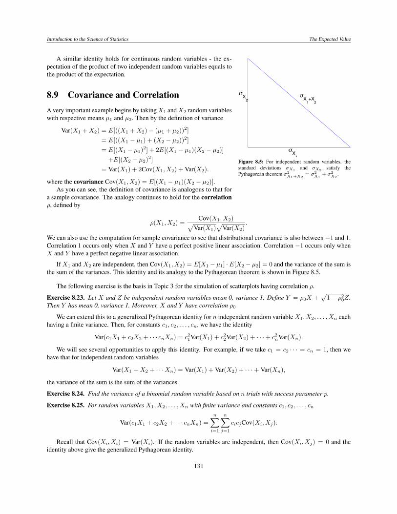
A similar identity holds for continuous random variables - the ex-pectation of the product of two independent random variables equals tothe product of the expectation.

8.9 Covariance and CorrelationA very important example begins by taking X

1

and X2

random variableswith respective means µ

1

and µ2

. Then by the definition of variance

Var(X1

+X2

) = E[((X1

+X2

)� (µ1

+ µ2

))

2

]

= E[((X1

� µ1

) + (X2

� µ2

))

2

]

= E[(X1

� µ1

)

2

] + 2E[(X1

� µ1

)(X2

� µ2

)]

+E[(X2

� µ2

)

2

]

= Var(X1

) + 2Cov(X1

, X2

) + Var(X2

).

where the covariance Cov(X1

, X2

) = E[(X1

� µ1

)(X2

� µ2

)].As you can see, the definition of covariance is analogous to that for

a sample covariance. The analogy continues to hold for the correlation⇢, defined by

⇢(X1

, X2

) =

Cov(X1

, X2

)

p

Var(X1

)

p

Var(X2

)

.

We can also use the computation for sample covariance to see that distributional covariance is also between �1 and 1.Correlation 1 occurs only when X and Y have a perfect positive linear association. Correlation �1 occurs only whenX and Y have a perfect negative linear association.

If X1

and X2

are independent, then Cov(X1

, X2

) = E[X1

� µ1

] ·E[X2

� µ2

] = 0 and the variance of the sum isthe sum of the variances. This identity and its analogy to the Pythagorean theorem is shown in Figure 8.5.

The following exercise is the basis in Topic 3 for the simulation of scatterplots having correlation ⇢.

Exercise 8.23. Let X and Z be independent random variables mean 0, variance 1. Define Y = ⇢0

X +

p

1� ⇢20

Z.Then Y has mean 0, variance 1. Moreover, X and Y have correlation ⇢

0

We can extend this to a generalized Pythagorean identity for n independent random variable X1

, X2

, . . . , Xn eachhaving a finite variance. Then, for constants c

1

, c2

, . . . , cn, we have the identity

Var(c1

X1

+ c2

X2

+ · · · cnXn) = c21

Var(X1

) + c22

Var(X2

) + · · ·+ c2nVar(Xn).

We will see several opportunities to apply this identity. For example, if we take c1

= c2

· · · = cn = 1, then wehave that for independent random variables

Var(X1

+X2

+ · · ·Xn) = Var(X1

) + Var(X2

) + · · ·+ Var(Xn),

the variance of the sum is the sum of the variances.

Exercise 8.24. Find the variance of a binomial random variable based on n trials with success parameter p.

Exercise 8.25. For random variables X1

, X2

, . . . , Xn with finite variance and constants c1

, c2

, . . . , cn

Var(c1

X1

+ c2

X2

+ · · · cnXn) =

nX

i=1

nX

j=1

cicjCov(Xi, Xj).

Recall that Cov(Xi, Xi) = Var(Xi). If the random variables are independent, then Cov(Xi, Xj) = 0 and theidentity above give the generalized Pythagorean identity.

131


8.9.1 Equivalent Conditions for IndependenceWe can summarize the discussions of independence to present the following 4 equivalent conditions for independentrandom variables X

1

, X2

, . . . , Xn.

1. For events A1

, A2

, . . . An,

P{X1

2 A1

, X2

2 A2

, . . . Xn 2 An} = P{X1

2 A1

}P{X2

2 A2

} · · ·P{Xn 2 An}.

2. The joint distribution function equals to the product of marginal distribution function.

FX1,X2,...,Xn

(x1

, x2

, . . . , xn) = FX1(x1

)FX2(x2

) · · ·FXn

(xn).

3. The joint density (mass) function equals to the product of marginal density (mass) functions.

fX1,X2,...,Xn

(x1

, x2

, . . . , xn) = fX1(x1

)fX2(x2

) · · · fXn

(xn).

4. For bounded functions g1

, g2

, . . . , gn, the expectation of the product of the random variables equals to theproduct of the expectations.

E[g1

(X1

)g2

(X2

) · · · gn(Xn)] = Eg1

(X1

) · Eg2

(X2

) · · ·Egn(Xn).

We will have many opportunities to use each of these conditions.

8.10 Answers to Selected Exercises8.2. For the fair die

EX2

= 1

2 · 16

+ 2

2 · 16

+ 3

2 · 16

+ 4

2 · 16

+ 5

2 · 16

+ 6

2 · 16

= (1 + 4 + 9 + 16 + 25 + 36) · 16

=

91

6

.

For the unfair dice

EX2

= 1

2 · 14

+ 2

2 · 14

+ 3

2 · 14

+ 4

2 · 1

12

+ 5

2 · 1

12

+ 6

2 · 1

12

= (1 + 4 + 9) · 14

+ (16 + 25 + 36) · 1

12

=

119

12

.

8.5. The random variable X can take on the values 0, 1, 2, 3, 4, and 5. Thus,

EX =

5

X

x=0

xfX(x) and EX2

=

5

X

x=0

x2fX(x).

The R commands and output follow.

> hearts<-c(0:5)> f<-choose(13,hearts)*choose(39,5-hearts)/choose(52,5)> sum(f)[1] 1> prod<-hearts*f> prod2<-heartsˆ2*f> data.frame(hearts,f,prod,prod2)

hearts f prod prod21 0 0.2215336134 0.00000000 0.000000002 1 0.4114195678 0.41141957 0.41141957

132


3 2 0.2742797119 0.54855942 1.097118854 3 0.0815426170 0.24462785 0.733883555 4 0.0107292917 0.04291717 0.171668676 5 0.0004951981 0.00247599 0.01237995> sum(prod);sum(prod2)[1] 1.25[1] 2.426471

Look in the text for an alternative method to find EX .

8.8. If X is a non-negative random variable, then P{X > 0} = 1. Taking complements, we find that

FX(0) = P{X 0} = 1� P{X > 0} = 1� 1 = 0.

8.9. The convergence can be seen by the following argument.

0 b(1� FX(b)) = b

Z 1

bfX(x) dx =

Z 1

bbfX(x) dx

Z 1

bxfX(x) dx

Use the fact that x � b in the range of integration to obtain the inequality in the line above.. Because,R10

xfX(x) dx <1 (The improper Riemann integral converges.) we have that

R1b xfX(x) dx ! 0 as b ! 1. Consequently, 0

b(1� FX(b)) ! 0 as b ! 1 by the squeeze theorem.

8.11. The expectation is the integral

Eg(X) =

Z 1

0

g(x)fX(x) dx.

It will be a little easier to look at h(x) = g(x)� g(0). Then

Eg(X) = g(0) + Eh(X).

For integration by parts, we have

u(x) = h(x) v(x) = �(1� FX(x)) = � ¯FX(x)u0(x) = h0

(x) = g0(x) v0(x) = fX(x) = � ¯F 0X(x).

Again, because FX(0) = 0, ¯FX(0) = 1 and

Eh(X) =

Z b

0

h(x)fX(x) dx = �h(x) ¯FX(x)�

�

�

b

0

+

Z b

0

h0(x)(1� FX(x)) dx

= �h(b) ¯FX(b) +

Z b

0

g0(x) ¯FX(x) dx

To see that the product term in the integration by parts formula converges to 0 as b ! 1, note that, similar toExercise 8.9,

0 h(b)(1� FX(b)) = h(b)

Z 1

bfX(x) dx =

Z 1

bh(b)fX(x) dx

Z 1

bh(x)fX(x) dx

The first inequality uses the assumption that h(b) � 0. The second uses the fact that h is non-decreaasing. Thus,h(x) � h(b) if x � b. Now, because

R10

h(x)fX(x) dx < 1, we have thatR1b h(x)fX(x) dx ! 0 as b ! 1.

Consequently, h(b)(1� FX(b)) ! 0 as b ! 1 by the squeeze theorem.

133


8.12. For the density function �, the derivative

�0(z) =

1p2⇡

(�z) exp(�z2

2

).

Thus, the sign of �0(z) is opposite to the sign of z, i.e.,

�0(z) > 0 when z < 0 and �0

(z) < 0 when z > 0.

Consequently, � is increasing when z is negative and � is decreasing when z is positive. For the second derivative,

�00(z) =

1p2⇡

✓

(�z)2 exp(�z2

2

)� 1 exp(�z2

2

)

◆

=

1p2⇡

(z2 � 1) exp(�z2

2

).

Thus,� is concave down if and only if �00

(z) < 0 if and only if z2 � 1 < 0.

This occurs if and only if z is between �1 and 1.

8.14. As argued above,

EZ3

=

1p2⇡

Z 1

�1z3 exp(�z2

2

) dz = 0

because the integrand is an odd function. For EZ4, we again use integration by parts,

u(z) = z3 v(z) = � exp(� z2

2

)

u0(z) = 3z2 v0(z) = z exp(� z2

2

)

Thus,

EZ4

=

1p2⇡

✓

�z3 exp(�z2

2

)

�

�

�

1

�1+ 3

Z 1

�1z2 exp(�z2

2

) dz

◆

= 3EZ2

= 3.

Use l’Hopital’s rule several times to see that the first term is 0. The integral is EZ2 which we have previously foundto be equal to 1.

8.16. For the larger order statistics, z(k) for the standardized version of the observations, the values are larger than

what one would expect when compared to observations of a standard normal random variable. Thus, the probabilityplot will have a concave upward shape. As an example, we let X have the density shown below. Beside this is theprobability plot for X based on 100 samples. (X is a gamma �(2, 3) random variable. We will encounter these randomvariables soon.)

8.17 For a single Bernoulli trial with success probability p, EX = EX2

= p. Thus, Var(X) = p� p2 = p(1� p).

8.18. For the fair die, the mean µ = EX = 7/2 and the second moment EX2

= 91/6. Thus,

Var(X) = EX2 � µ2

=

91

6

�✓

7

2

◆

2

=

182� 147

12

=

35

12

.

For the unfair die, the mean µ = EX = 11/4 and the second moment EX2

= 119/12. Thus,


=

119

12

�✓

11

4

◆

2

=

476� 363

48

=

113

48

.

8.19. For the dart, we have that the mean µ = EX = 2/3.

EX2

=

Z

1

0

x2 · 2x dx =

Z

1

0

2x3 dx =

2

4

x4

�

�

�

1

0

=

1

2

.

134


0.0 0.5 1.0 1.5 2.0 2.5 3.0

0.0

0.2

0.4

0.6

0.8

1.0

x

dg

am

ma

(x,

2,

3)

-2 -1 0 1 2

0.0

0.5

1.0

1.5

2.0

2.5

Normal Q-Q Plot

Theoretical Quantiles

Sa

mp

le Q

ua

ntile

sThus,


=

1

2

�✓

2

3

◆

2

=

1

18

.

8.20. If t < �, we have that e(t��)x ! 0 as x ! 1 and so

MX(t) = EetX = �

Z 1

0

etxe��x dx = �

Z 1

0

e(t��)x dx =

�

t� �e(t��)x

�

�

�

1

0

=

�

�� t

Thus,

M 0(t) =

�

(�� t)2, EX = M 0

(0) =

1

�,

andM 00

(t) =2�

(�� t)3, EX = M 00

(0) =

2

�2

.

Thus,Var(X) = EX2 � (EX)

2

=

2

�2

� 1

�2

=

1

�2

.

8.21. ⇢X(z) = EzX =

P1x=0

P{X = x}zx The k-th derivative of zx with respect to z is

dk

dzkzx = (x)kz

x�k.

Evaluating at z = 1, we find thatdk

dzkzx�

�

�

z=1

= (x)k.

Thus the k-th derivative of ⇢,

⇢(k)X (z) =1X

x=0

(x)kP{X = x}zx�k and, thus,

⇢(k)X (1) =

1X

x=0

(x)kP{X = x} = E(X)k.

135


8.22. Let EX = µ. Then the expected value E[aX + b] = aµ+ b and the variance

Var(aX + b) = E[((aX + b)� (aµ+ b))2] = E[(a(X � µ))2] = a2E[(X � µ)2] = a2Var(X).

8.23. By the linearity property of the mean

EY = ⇢0

EX +

q

1� ⇢20

EZ = 0.

By the Pythorean identity and then the quadratic identity for the variance,

Var(Y ) = Var(⇢0

X) + Var(q

1� ⇢20

Z) = ⇢20

Var(X) + (1� ⇢0

)Var(Z) = ⇢20

+ (1� ⇢20

) = 1.

Because X and Y both have variance 1, their correlation is equal to their covariance. Now use the linearity propertyof covariance

⇢(X,Y ) = Cov(X,Y ) = Cov✓

X, ⇢0

X +

q

1� ⇢20

Z

◆

= ⇢0

Cov(X,X) +

q

1� ⇢20

Cov(X,Z)

= ⇢0

· 1 +q

1� ⇢20

· 0 = ⇢0

8.24. This binomial random variable is the sum of n independent Bernoulli random variable. Each of these randomvariables has variance p(1� p). Thus, the binomial random variable has variance np(1� p).

136

Documents

The Expected Value - University of Arizonamath.arizona.edu/~jwatkins/H_expectedvalue.pdf · Topic 8 The Expected Value Among the simplest summaries of quantitative data is the sample