•

THE EXPECTATIONS OF MEAN SQUARES

by

R. E. Comstock

Institute of Statistics

Mimeograph Series No. 76For Limited Distribution

:,,/t I'f'! ! 1"""-~ . 'j) ,;

Chapter VI

ThL r.,XP.c.CTATIONS OF ML;AN SQU.l~

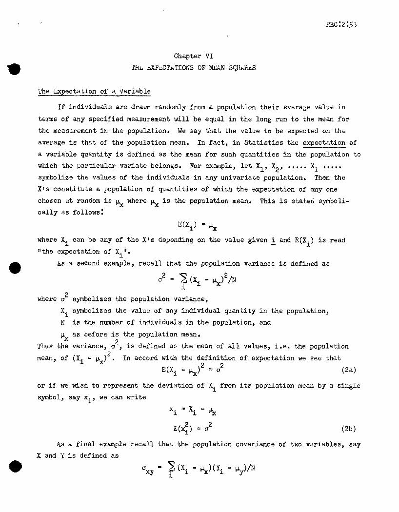
The Expectation of a Variable

If individuals are drawn randomly from a population their avera3e value in

terms of any specified measurement will be equal in th8 long run to the mean for

the measurement in the population. We say that the value to be expected on the

average is that of the population mean. In fact, in Statistics the expectation of

a variable quantity is defined as the mean for such quantities in the population to

which the particular variate belongs. For example, let Xl' X2

, ••••• Xi •••••symbolize the values of th8 individuals in any univariate population. Then the

XIS constitute a population of quantities of which the expectation of anyone

chosen at random is ~ where IJ. is the population mean. This is stated symboli-x xcally as follows:

E(X.) = IJ.~ x

where X~ can be any of th~ XIS depending on the value given i and E(l.) is read... - ~

"the expectation of X.".~

As a second example, recall that the population variance is defined as

2 ~ 2(J = .~ (Xi - IJ.) /N

i

(2a)

population

see that

8~mbolizes the population variance,

X. symbolizes the value of any individual quantity in the population,~

N is the number of individuals in the population, and

as before is the population mean.. 2. d f' d th f 11 1 . hvarlance, (J , ~s Slne as e mean 0 a va ues, 1 0 e. t e

2(Xi - IJ.x) • In accord with the definition of expectation we

E(Xi - IJ.x)2 = i

IJ.xThus the

mean, of

or if we wish to represent the deviation of Xi from its population mean by a single

symbol, say xi' we can write

X • ." X. - ~x~ ~

(2b)

As a final example recall that the population covariance of two variables, say

X and Y is defined as

(J = ~ (X. - IJ. )(Y. - IJ. )/Nxy i 1 X ~ Y

-2-

where cr is the covariance ana other symbols have meanings in conformity withxythose listed above when considering the variance of X. We see that the covariance,

a , is defined as the population mean of (X. - ~ )(y. - ~ ) and therefore thatxy ~ x ~ y

Again if we set

we can write

and y. z: Y. - jJ.~ ~ y

E(x.y.) = cr~ ~ xy

crxy (3a)

(3b)

Interest in expectations centers around the fact that by setting observed

quantities equal to their expectations we find a basis for unbiased estimation of

parameters involved in the expectation. For example, it can be shown that

E(X. - 1)2 = n-l i~ n

It follows that

where Xis the mean of a sample of XIS, and

n is the number of individuals in the sample.

E I~ (X. - j{)J . n(n-l) i = (n~=l ~ J n

- 1) i

orr- n

X)2 °1~

E ls2 ~ (x. -2= = a

i=1 ~ In-l J

From this we see that sample variance obtained by dividing the sum of squares by2degrees of freedom has cr as its expectation, i.e. that it provides on unbiased

estimate of i.

Expectation of a Constant

This is specifically mentioned for completeness. Since a constant, by defi­

nition, is a quantity that always has the same value, the expectation of a constant

could hardly be anything but that particular value. For example, a population mean

is a constant and its expectation is the mean itself. Symbolically, if c is any

constant,

1(c) = c (4)

-)-

e .li.xpectation of the Product of a Constant and a Variable

Consider the product

Y '" c X

where X is a variable and c is a constant. We know that the population mean of Y

is c ~x and, tberefor~,

E(Y e C X) '" c ~ = c E(X)x (5)

In g6neral, the expectation of such a product is the product of the constant and

the expectation of the variable.

The Expectation of a Linear Function

Consider the linear function

F '" a + b + c Xl + X2

in which ~, £. and c are constants and Xl and X2 are variable qUJrlti ties drawn

randomly (but not necessarily independently) from two populations (one, a popu­

lation of quantities symbolized as Xl' the other a population of quantities sym­

bolized as X2). Two points are worth special attention.

(1) The specific manner in which F is definod may have the result that value~

of Xl and 12 contributing to different values of the quantity, F, are

correlat~d or on the other hand are independent, i.e. uncorrelated. For

example, suppose F is designed to reflGct in some special way the h6ight

of married couples. Then any single value of F would involve the height

of the husband (Xl) and that of his wife (X2). If the couples are chosen

randomly both Xl and X2 are random values from their respective popula­

tions, but art not necessarily independent in magnitude from one couple

to anothero In fact, evidence indicates that there is a degree of corre­

lation in stature of man and wife.

On the other hand, suppose F were defined as the h8ight of plants,

Xl as ti-!.,;: effect of genotype, and ~ as the effect of environment on

height; and it were known that in the population of plants involved geno­

types were distributed randomly with rl:Jspect to environment. The magni­

tudes of Xl ill1d X2 would vary independently from plant to plant and,

therefore, from one valub of F to another.

-4-

(2) The different variables may actually belong to the sam~ population

though it may be useful to think of them as coming from different ones.

For example, in the function given above Xl and X2 could be a pair of

values drawn randomly from the same population, Xl' being the first and

X2 the second drawn of any pair. In this case Xl and X2 would vary

independently, i.e. be uncorrelated.

Corresponding to every possible pair of values of Xl and ~ there is obviously

a value of F. These values comprise a population of F's. iie know that the mean

value of F in that population is

a ... b +c!J.l +~2

where ~l and ~ are the population means for Xl and X2, respectively. Hence

E(F) = !J.F a a + b + c !J.l + !J.2

where !J.F is the population mean of F. This serves to demonstrat~ the general fact

that the 6xpectation of ~ variable quantity~ is ~ linear function of other

variables is the~ linear function of ~ expectations of those variables. By

this rule

E(F) : E(a) + E(b) + E(c Xl) + E(~)

and since

E(a) = a

E(b) =b

E(c Xl) = c 1J.1

E(Y.2) = 1J.2

1,je have by substitution

E( F) = a + b + C !J.l + 1J.2

as given above.

Expectations of hcan Squares

Any mean square can be writt8n as a linear function in which the variable

quantities are the squares of variables, products of a variable with a constant, or

products of variableS. Bbnc~, the expectations can always be written in terms of

what is presented above. This fact will b~ clarified by examples.

-5-

Example I

Consider thG case rtp~es~nted by the analysis of variance for comparing

groups of equal size. The form of the analysis is as follows:

Variance Source

Groups

Within groups

Total

d.fo

m-l

m(n-l)

m n-l

m.s.

where m is the number of groups and n is number of individuals within groups. The

model on which the analysis is based can be stated symbolically as follows:

Y.. = jJ. + g. + e ..1) 1 1J

where ~ is the population mean taken over all groups,

gi isthe effect of the i-th group (the amount by which the ~opulation mean

for the i-th group deviates from ~), and

e .. is a random effect contributing to tht valu8 of Y for the j-th individuallJ

in the i-th group (the amount by which the individual deviates from the

mean for its group),

One of two assumptions is usually made concerning the groups: (a) that they

are random members of a population of groups, or (b) that the ones on which data

are taken are of special interest in themselves rather than as a sample from a

population. In case (a) the assll.'1lpt.io:1. is frequently stated by saying that g. is1

considered a random v3.riabl<.., in con7..:;.'at:' to case (b) where it is alternatively

said that the g. arc considered constant or fixed.1

g assumed to be a random variable

~e will consider first the case where g. is consid0red a random variable.1

G. be the sum of Yls for the N individuals of th~ i-th group, and1

T be thE.. sum of Y's for all nm individuals on which data were collectedg

Then thG mean squar~

T2

- /m-lnm

(6)

-6-

1 .This may b~ considtred the product of a constant and a variable where ~ 15 them-.Lconstant and the quantity in brackets is the variable. Hence, its expectation may

be written,

1 ,[12 2 2E(Ml ) '" m-l E :n (Gl + G2 + .... Gm)

122 2Note that :n (Gl + G2 + •••• Gm) is "That we commonly call the "uncorrected sum of

squares", that T2/nm is what we call the "correction factor", and that the whole

quantity in brackets is the "corrected sum of squares".

By the rule that the expectation of a linear function is the same function of

~xpectations of the variables in the function, we can write

1 [1 2 2 2 1 21E(Ml ) ... m-l .:n(EGl + EG2 + .... EGm) - run ET j

.... 2

+ Y'2 + •••• Y. J1 1n

Now the separate expectations in the expression can be considered

Consider EG~. In terms of our model,1

EGi •EL~l Iij] 2•E[In

one by one.

.E(n~ + ng. + e' l + e'2 +111

2• • •• e. )1n

Squaring and taking expectations term by term this can be written

'~G2 En2 2 En2 2 E{.t. 1i = ~ + gi + eil + ei2 + ••••2e. )

1n

+ •••• e. )1n

(7)

Before going further note, that both the g I S and e I s are defined as deviations from

a mean and hence, that the population mean of both the gls and e's is zero. Thus,

E(g.) ... 0, E(e .. ) D 0, E{g~) = 02 and B{e~.) = 0

2 where 02 is the population vari-

1 1J 2 1 g 1J e g .ance of g's and cr is the population variance of e's. It is common to assume thateall els are members of the same population and, therefore, that 0

2 is homogeneouseover all groups. This assumption will be made for the purpose of our example but

it should be understood that special cases may arise where the variance of e variese from group to group. It should also be noted that all g' sand e I s are assumed to

-7-

be random members of their populations. The significance of this is that in th~

population (the population that would be generated by repeating the experiment in

identical fashion an infinity of times) the correlation between (1) any two gIs,

(2) any e's, or (3) any ~ and any ~ would be zero. If the correlation is zero, so

also is the covariance and this means that the expectations of all products of two

gIs, two e's or a Kand an e are all equal to zero. Symbolically this is stated

as follows:

E(g. g!) "" 01. 1. (i f i' )

E(e .. et I,) =01.J 1. J (ir i ' ifj =j',jrj' ifi=i')

E(g,' e, ,) = 01. 1.J (either when i = i' or Wben i , i')

Now let us consider the

2IS (1 )

g

••••

2s~veral terms of EGi one by one.

(since n2~2 is a constant)

(since n2 is a constant)

(since Egi2

•••• Sin)

"" n2 Ei1.2 2

"" n (1g

2 2... n IJ. •.. 2 2J:!,njJ.

2 2E n gi

(a)

(b)

(c)

+ ••••

::md')

is (J£.en of them,

(d)

... n(1~ (since thu expectation of each of the 62

,S,

that of each product term is zero)

E2n2IJ.g, ... 2n2~g. (sinc~ 2n21J. is a constant)1. 1.

... zero (since Egi = 0)

(e) E2nIJ. (ei1 + 8 i2 + •••• Sin)

... 2n~ (eil + ei2 + •••• ein) (since 2n~ is a constant)

= z~ro (since the expectation of all e's is zero and, therefore, that

of the sum of any set of e's is also zero)

(f) E2ng, (e'l + b i2 + •••• e. ) ... 2nEg . «(;'1 + (;. 2 + •••• e. ) (sinct;: 2n is1. 1. 1.n 1. 1. 1. . 1.n a constant)

• Z0ro (since the expectation of the product of any ~ and ~ is zero)

REC:2:5J

-8-

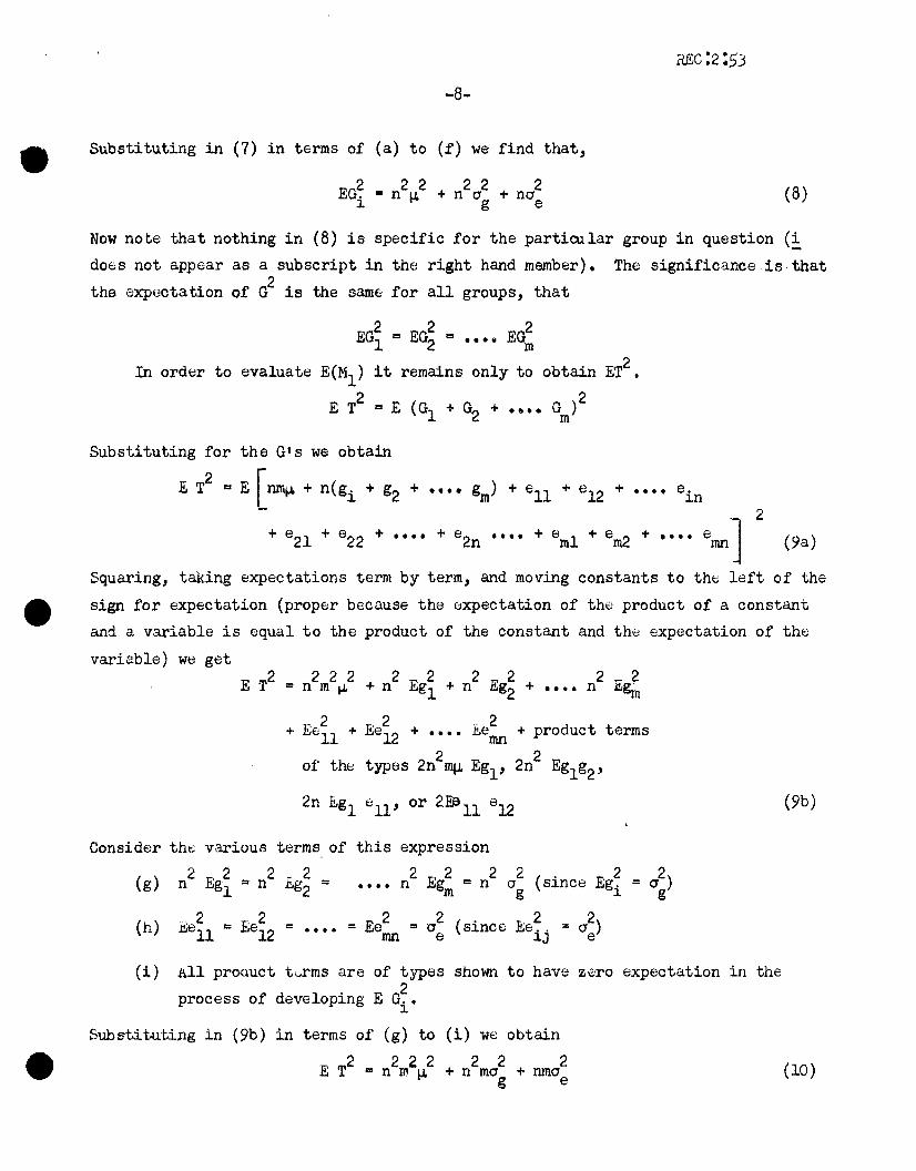
Substituting in (7) in terms of (a) to (f) we find that,

22222 2EG. = n ~ + n a + na~ g e (8)

Substituting for the GIS we obtain

E T2 = E [~ + n(gi + g2

Now note that nothing in (8) is specific for the particular group in question (!does not appear as a subscript in the right hand member). The significance is-that

the expectation of G2 is the same for all groups, that

EGi = EG~ = .... EG;

In order to evaluate E(Ml ) it remains only to obtain ET2

•

E T2 = E (Gl + G2 + •••• Gm

)2

2+ e2l + e22 + .... + e2n .... + eml + em2 + •••• emnJ (9a )

Squaring, taking expectations term by term, and moving constants to th~ left of the

sign for expectation (proper because the expectation of the product of a constant

and a variable is equal to the product of the constant and the expectation of the

variable) we get2 222 2 2 2 2 2 2E T = n m ~ + n Egl + n Eg2 + •••• n E~

E 2 E 2 - 2 d t t+ -ell + e12 + •••• ~emn + pro uc erms

2 2of the types 2n m~ Egl , 2n Egl g2,

2n E.gl ell' or 2~11 8 12

Consider thE. various terms of this expression

(g) 2 Ei = n2 _ 2 2 E 2 2 2(since Eg~ ri)n .c.g2

= •••• n gm = n (J =1 g g

(h) . 2 E 2 2 2 (since Ee~. = i)J::!,ell

c: e12 = •••• = Ee = C1

mn e ~J e

(i) all proauct torms are of types shown to have z~ro expectation in the

process of developing E G~.~

(9b)

Substituting in (9b) in terms of (g) to

E T2 2 2 2

=nrotJ.

(i) we obtain

222+ n ma + nmag e (10)

-9-

Finally substituting in (6) in terms of (8) and (10) we find

1 [m 2 2 2 2 2 1 2 2 2 2 2 2]E(M ) ... ~ - (n II. + n a + no ) - - (n m:1. + n mO" + nma1 m-~ n ~ g e nm ~ g e

2 l-mn-mn] 2 rmn-n] 2 l- m-lJ 2, 2... ~ m-r + ag ~m-r + ae m-l = nag + aE:

The within group me~n square may be computed as follows:m 02

1 ~ 2 u2 _2 1M2 = ( 1) ~ (Y' l + ~2 + •••• ~ ---)m n- . 1 J. J. J.n nJ.=

(11)

(12 )

RcmE:mbering (a) that the expectation of the product and of a constant and a vari­

able is thE. product of the constant and the expectation of thE; varic::blt: and (b)

that tht: E:xp~ctation of a variable that is a linear function of variables is the

same function of the expectations of these later variables, we se& that

E(~) z m(;-l} ~l [E~l + E~2 + •••• E~n - ~ Eoi]2Consider the expectation of Yij

Therefore,

E1:, • E(~ + g. + 6 i .)2J.J J. J

Expanding ~nd taking expectations of individual terms separately we obtain,

Ei, = E~2 + Eg~ + Ee~, + E 2~g. + E 2~e .. + E 2g.e.. (13)J.J J. J.J J. J.J J. J.J

Taking the terms of this 6xpr0ssion separately,

(j) E~2 ~ ~2 (bbcausG ~2 is a constant),

(k) Ei = i (by definition when thcl g's arE.: assum8d random),J. g

(1) Ee~, = 02 (by definition),J.J e

(m) E 2~g. = 2~ Eg. = zero (since 2~ is a constant and Eg. = 0),J. J. J.

(n) E 2~e .. = 2~ £8., ... Z8ro (since 2~ is a constant and Ee'iJ' = 0),J.J J.J

(0) E 2g.e., ... 2 Eg.e .. = zero (since 2 is a constant and Eg.e., a 0).J. J.J J. J.J J. J.J

Substituting in (13) in terms of (j) to (0) we obtain,

;;'y2 2 2 2l~ .. =1-.1. +0 +0

J.J g e (14)

-10-

2We have already shown (8) that the expectation of Gi is,

E G~ ,.. n21J.2 + n2i + nei (8 )1 g e

Note that both (14) and (8) are the same for all Y's and GIS, respectively (all

terms in right hand members are constants). Recognizing this and substituting in

(12) in terms of (8) and (14) we obtain,

E(~) • m(:-l) [n(~2 + <7~ + <7~) - ~(nV + n2<7~ + n<7;)l

- 2 f'rn(n-n) -J + ei [m(n-n) ] + ei [m(n-l)l Ul cl (15)- lJ._m(n-l) g men-i) e _m(n-l)-. e

Using (11) and (15) the analysis of variance can now be pr~sented giving t~e

expectations of the mean squares.

Variance Source

Group·s

Within groups

Total

d.f.

m-l

m(n-l)

mn-l

Expectation of m.s.2 2

(j + n(je g2

(je

~~~ assumed to be constants

Differ~nces occasioned by assuming the gls constant rather than random are

listed below.

gls random gls constant

E g1 = 0 E g. :; g.1 1

E 2 2 Ei 2=(j = gigi g 1

Bcg. = 0 Ecg. = cg.1 l. 1

where c is any constant

other expectations involv8d in (7), (9b), and (13) are not affGcteo. ~'iith

the above differences in mind we s~& that in this case (7) does not reduce to (8)but to

E G~1

(16)

In like manner (9b) reduces to

222 2E.T =nmlJ. 2+ nm(je (17)

-11-

rather th<l.n to (10). The reason why no terms involving gls or the squar·:;s or

products of gls occurs in (17) is clarified by refer6nce to (9a). Note that the

gls ent~r (9a) in a tarm that is the sum of th8 gls for the ~ groups. In the caS6

where; ths g I S are assumed constant tJ. is taken as the population mean for the ~

groups in qU0stion. Then, since the gls are defined as deviations from this mean,

th~ir ~um must be zero. Hence, the term n(gl + g2 + •••• gn) disappears from (9a)

and correspondingly t~rms involving gls disappear from (9b). Finally (13) reduces

to(18)

[

m m1 1 2 2 2'~ 2 2'" 2

E(Ml ) = - -(ron j.L + n ..::::; g. + 2n jJ. ~ g~ + nmoe )m-l n . 1 ~ . 1 ...~= 1'"

rather than to (14).Substituting in (6) in terms of (16) and (17) rather than in terms of (8) and

(10) we obtain,

m

Keeping in mind that :2 g. I:: 0 as pointed out above this reduces toi==l J.

r~?-.!~ 1.1 m,,·J.- ~

m

+~ 2: i.l.' + a:m-l ""i=l [m-11m-l _

(19)

Substituting in (12) in t,:;rms of (16) and (18) rather than in terms of (8)

and (14) we obtain,

m m1 2 2 2~ 2 2 ~- - (mn jJ.. + n ~ g. + 2n u. ~ g.n i=l .1. i=l .1.

f, 2

._ \lTlniJ. + n2

g. + 21J.I1~

m

~i=1

2g. + mna ).1. e

+ mna~]

2= ,J.[

n-n ]_nl(n-l)

2+ a

E;;

2'" (Je

(20)

-12-

m

~ie have again used the fact that ~ g.i=l ~

tatiom is now as follows:

= o. The analysis of variance with GXp0C-

Variance Source

Groups

d.f.

m-l

Expectation of m.Q.m

2+..£... ~ 2O"e m-l .~ gi

1=1

TNithin groups m(n-l) 20"e

Total mn-l

Example 2

As a variation of example 1 consider th~ analysis of variance for comparison

of groups of unequal size. Let nl , n2

•••••• nm symbolize the number per group

in groups 1, 2, •••••• m, respectively. Th~ form of th~ analysis is as follows:

Variance Sourcf:) d.f. m. s.

Groups m-l Mlm

Hithin groups ~ (ni-l)i=l

Total N-l

wher\:J N is the total numb"r of individuals in all groups.

(21)

the same as in example 1.

random variahle. The mean

group size the model will be

case where ~ is considered a

c:mlP:tc:1a[s G~ + ::L .... G~_m- nl n2 nm

Lxcept for variation in

will consider only the

square for groups is

R.eferring to (7) and (8) it is clear that

E G~ 2 2 2 2 2= n. ~ + ni 0" + n. (j

~ ~ g ~ e

and hbnce that2 2 2 2 (22 )E(G. In. ) =n1 jJ. + n. 0" + 0"J. J. J. g e

-13-

'l' is now equal to

N~ + n1g1 + n2g2 + •••• nmgm + ell + 8 12 + •••• sln1

+ e21 + 8 22 + •••• e2n2 + •••• e 1 + e 2 + •••• em m mnm

Squaring and taking expuctations but ommitting t~rms with ~xp~ctation zero we obtain,

222.22 2222E T '" N t.l. + E n1

g'l + E nz g2 + •••• + E nmgm

E 2 ~ 2 E 2+ ell + ~ 6 12 + •••• + sln +

1

222•••• E em1 + E 8m2 + •••• + E t mnm

Evaluating thb s~parat~ terms, this becomes

E T2 • N2,,2 2 2 2 2r"' + n10'g + n20'g +

and. hence, m2 2 2 ~ 2 2

E(T IN) = N~ + 0' .z n. IN + 0'g i"'l 1. e

(23 )

2 2lJic have NO'e bbcause there are a total of N terms of the type 1e11 that art-' equal

m

Ni - i ~ n~/N -g i=l 1.

2to 0' •e Writing E(M1) in tbrms of (21), (22), and (23) we

E(M1) '" m~l [i ~ ni + i g ~ ni + mO";i"'l i=l

mNoting that ~ n. = N, this reduc0s to

i=l 1.

get

(24)

The coefficient of 0'2 in (24) is of the same form as given by Sn~docor (p.234, 1948).g

The within group mean square is computed as

+ •••

-14-

M2 • N~m [i!• N~m f'til + ti2 + ....

+ ~l + ~2 + .....f )-mnm

'raking the expectation term by term we have

E(~) • N~m [Etil + Ei112 + .... Ei1ln1

+ E~l + E~2 + .... E~~

+ Ei.fml + E~2 + •••• E.fmn - EG~/nlm

(25)

The L-xpectation of the square of any single Y is in no way affect8d by the numb(~r

= N, this reduces to

m

~ n. jJ.i=l J.

of individuals obs~rv8d in each group. Therefore, it is

tuting in (25) in terms of (14) ,md (22) we obtain,

E(~'2) • N~m tfL2

+ N"~ + N"~ •

m -

- ~ n. i - miJ1=1 J. g em

Rdmembering tha t jJ. and i arE; constan ts and that ~ n.g i=l J.

giv6n by (14). Substi-

(26)

R~f8rring to (24) and (26) the analysis of variance with mean square 8xp0ctations

can now bo writtbn as follows:

VariancE: Source

Groups

Within groups

-15-

d.f.

m-l

N-m

Bxpcctationc of m.s.

r::l + n t r::le g

Genoral Procedures

Total N-l

~ 1where n ". ~m-J.

m-.:'1 2--~ nii=l

N - --;:NO;---

Before turning to other examples it will be useful to summariZ8 the general

procedures demonstrat0d in the foregoing examples. Steps in th8 procedure are list8d

b,;;low.

1. Specification of the model. This includes a symbolic statement of the

composition of the individual values that make up th0 data, assumptions

as to whether the various ~ffccts are fixed or random, and assumptions

concerning whether separate 8ffects vary independently.

2. Th~ composition of each moan square is written out in terms of the mod~l

and the steps followed in computing the mean square~

3. The expectation of the mean square is developed term by term.

Rules employed in step 3 may be summarized as follows.

1. The expectation of a constant is thu constant itsolf.

2. The 6xp~ctation of ~ variable is the population mGan of the v~riable.

3. The expectation of the square of a variable '~hat has population mean zero

is the population variance of the variable.

4. The expectation of tht product of a constant and a variable is the product

of the constant and th~ expectation of the variable.

5. The expectation of th6 product of two variables that have population mean

zero is the population covariance of th0 variables.

6. The population covariance of any two variable effects is zero whenever

the particular two effects contributing to any OnE) m(;asur~ment in thi'j

data may be assumed to bejn~ drawn from their respective popu­

lations.

-16-

Two points merit special attention.

1. It is d6sirable to write the model in terms of a gen~ral mean so that all

effects will have zero as thdr popula.tion m8an. This allows taking

advantage of 3 and 5 above.

20 If 6 aboVe is kept in mind a great deal of labor can bo saved, in writing

out the composition of m",an squaros in expanded form, by omittingprcd\\cJG ....

terms that have expectation zero. For example with this in mind (7) might

have been written

2222222E G. = E n ~ + Eng. + E e'l + E 8'2

~ ~ 1 ~+ ••••

2E e.1n

for thE. case where g. was consided a random variable.1

In the case of more complicated analyses than thoSG considered in the fore-

going examples, expressiuns for the composition of the various mean squares may

be v~ry long. Rather than follow the procedure outlin6d above in just the form

demonstated by examp16s 1 and 2.t it is more conVenient in these cases to recognize

that every m~an square can be computed as a linear function of one or mor~

"uncorrected" sums of squares and what is commonly called the correction factor.

Thus the expectation of a mean squarE. can be obtained by combining the bxpectations

of uncorrected s~~s of squar~s and the corrbction factor in the same way that the

sums of square and correction factor were combined to obtain the mean square. The

procedure is to find the expectations of the uncorrected sums of squares that must

be computE:Q in the analysis and of the correction factor and then combine these

appropriately to obtain th~ 8xpectations of the mean squares.

Example 3

Consider the analysis of data obtained from comparison of ~ gcn6tic strains of

a particular annual crop in a randomized block design at each of s locations in each

of ! years. Assum8 ~ roplications in each location each year and that diff8rent

land or at least a new randomization is used in succ8ssive years at each location.

The form of the variance analysis is as follows:

-17-

Varianc;;; Source d.f. .. -m.s.

Locations

Years

Lx Y

Reps in years and locations

Strains

L x Strains

Y x Strains

L x Y x Strains

Strains x reps in Land Y

Total

Th.., modGl employcd will be as follows:

s-l

t-l

(s-l)(t-l)

st(r-l)

n-l

(s-l) (n-l)

(t-l)(n-l)

(s-l)( t-l)(n-l)

st(r-l) (n-)

rstn-l

y, 'kl =~ + g. + a. + bk + (ab)'k + (ga),. + (gb)l.'k~J ]. J J ].J

+ (gab) , 'k + c, kl + (gc)., kll.J J l.J

wh8re ~ is th8 population mean

is thG effect of the i-th strain

(gab)ijk

is the effGct of the j-th location

is the tffect of the k-th year

is an 0ffoct arising from first order int~raction betw8en ~nviron­

ment conditions of the j-.th location and k-th year

is an effect arising from first order interaction of the i-th strain

wi th the j -th location

is an 8ffcct arising from first ordGr interaction of the i-th strain

with the k-th year

is an &ff6ct arising from second order interaction of the i-th strain

with the j-th location and k-th year

is the effect of the l-th block at the j-th location in the k-th

year as a deviation from th6 mean for that location and year, and

-18-

(gc), 0kl is the effect of the plot to Which the i-th strain is assignbd in1.J

the I-th block in the j-th location and k-th year (strictly speaking

it also contains a plot~strain interaction effect and the error of

measurement, but only in special cases would it be important to

indicate this sub-division in the model).

All effects will be considered random variables with mean zero. This would be

appropriate if the objective of the work was to compare the strains for use in

locations and years of which those involved in the experiment were a random sample,

and if th~ strains represented a random sample from a population from which other

strains might have been taken for comparison. It will also be assumed that all

effects vary randomly with respect to each other so that all covarianc6s among

pairs of 8ffccts are ZEro. This is an appropriate assumption in consideration of

th~ way work like this is usually conducted. Finally, it will be assum6d that

E(ga)~ , is constant OVtlr all values of i and j1.J

. 2 is constant all values of i and kE(gb)ik over

2 is constant all valu6s of j and kE(ab)jk oVt:r

2 is constant all values of i, j, and kE(gab), 'k OVt;r1.J

2 is constant all values of j" k" a.nd 1E cjk1 ovt::r

2 is constant all values of i, j, k, and 1.E(gc) 0, kl over1.J

The sense of this is that all individual EJff6cts within anyone of th8 six kinds

belong to a common population and have the variance of that population as the

Qxpectation of their squares. This is an assumption very commonly made in connec­

tion with analyses of the typE; in question, though it may not always be justified.

The letter T with appropriate subscripts is used to symboliZE: different sums

of the Y's. For example,

T =grand total

Ti = sum for the i-th variety (over all locations, years, and blocks)

T. = sum for the j-th location (over all strains, years, and blocks)J

Tij .. sum for thE: i-th strain at thE; j -th location (over all years and blocks)

E:tc.

-19-

Carriud to its ultimat6 this means

but Yijkl will be used instead of Tijkle The uncorr~ct~d sums of squares will be

symbolized by S with appropriate subscripts. For 8xample,

S = T2/nrst = the correction factor.n

= ~ T~/rst = uncorrected sum of squares for strains.i=l ~

n sS.. ... ~ ~ T~ ./rt = uncorrected sum of squares for strain-location totals,~J i=l j=l ~J

etce

The process of obtaining thE; expectations of the mean squar(;s can be amply

illustrated by considering only one mean square, say M2. It is computed us follows:

1[Sij - (Si - S) - (Sj - 5) - sl~ -- (n-i{s-l) -

1[Sij - S. - Sj + s]= (n-l) (s-l) ~

Consequently1

E(M2) ... (n-i)(s-i) rE S.. - E S. - E S. + E slLJkJ ~ J -

(27)

The SIS involved have th8 following composition

SiJ' = ; ~ ~ T~ .r i j ~J

S. 1 ~T~=-J nrt j J

5 1 T2=-nrst

-20-

It follows that their expectations arB,

E Sij1~

.~ 2

\=- ~ E Tijrt i j

I

E S. 1~ E T~

~ :: rsti ~

E S. 1 ~ E T~""-J nrt

j J

E S "" -l:...- E T2nrat

4S the basis for obtaining the expccta tions of the TIS w~ must !mow their com­

position. The expectation of the square of any of th~sc TIs,

TJ.'j :: ~ ~ y, 'ldk 1 J.J

T. :: :2~~ YijldJ. j k 1

T. = 2~~ YijklJ i k 1

(28)

T ...

Expanding th8se sums in terms of the model for the analysis we have the following:

TJ.'J' = rt~ + rtg. + rta. + r

1.. J

+ r ~ (gab) .. k + ~~k J.J k 1

~ bk + r ~ (ab) 'k + rt(ga) ..k k J J.J

c . kl + ~] (go)., klJ. k 1 1.J

+ r ~ (gb). kk 1.

Ti :: rstiJ. + rstgi + rt ~ a.j J

+ rs ~ ~~~ (gb). k + r _ ~k 1. j k

+ rs ~ bk + r .~ ~ (ab) 'k + rt ~ (ga) ..k j k J j J.J

(gab), 'k + ~ ~ ~ c'kl + ~ ~ ~ (go)"kl1.J j k 1 J j k 1 J.J

-21-

T. = nrt~ + rt ~g. + nrta. + nr 2bk + nr ~ (ab)'k + rt Z (ga) ..J i 1 J k k J i 1J

+ r f f (gb)ik + r ~ .~ (gab) .. k + n ~ ~ c. kl + ~ ~ ~ (gc) ..kli k 1J k 1 J i k 1 1J

T =s nrst~ + rst ~ gi + nrt ~ a. + nrsi j J

+ rt ~ ~ (ga) .. + rsi j 1J

+ ~ ~ ~ ~ (gc)'jkli j k 1 1.

~ ~ (gb) 'k + ri k 1.

~ bk + nr ~ ~ (ab) . kk j k J

ZZ~ (gab) .. k + n ~ ~ ~ C . klij k 1.J j kl J

The expectation -,f' :" .. of the square of any of these T's is thb sum of the expecta­

tions of each term in the square. however, since all covariances among different

effects are Zbro (see statement of model) the expectations of all product terms in

the square of any T are also zero. Thus only the expectations of the squares of

thG separate terms in the above expressions o.:mtribu'b<.; to the expectations we ar8

seeking. These can be written directly from inspection of the terms. For example,

2t

2 2'" r tL

2wh6re cr s~~bolizes th~ population variance of the.bffect indicated by subscript

(bocause (1) the numbor of bls in the sum indicated

is t, (2) Eb~ = cr~, and (J) the expectation of the

product of two bls is zero)

Proceeding in this way the expectations can be written from the equations for the

T's as follows:

2t 2 2 2t 2 2 2t 2 2 2t 2 2t 2 2t 2 2 2t 2.. r lJ. + r crg + r cra + r crb + r crab + r ~ga + r crgb

+ r 2ti b + rti + rtiga c go(29a)

-22-

b T~ 2 2t 2 2 2it22 22222 2 2 2 2 t2 2=rs eJ. + r a + r st aa + r stab + r staab + r s a~ g ga

222 2 2 2 2+ r s tagb + r sta b + rstO' + rstO'ga 0 go

E T~ 2 2t 2 2 222 + 2 2t 2 2 222 222 222=nr IJ. + nr t 0' n r cr + n r to'b + n r taab + nr t 0'J g a ga

2 2 2 2 2 2 2+ nr tagb + nr tcr b + n rtcr + nrtO'ga 0 go

(29b)

(29c)

22222 2222 2222 222222 2= n r s t tJ. + nr s t 0' + n r st 0' + n r &I 'to:b +n r stO' bg a a

nlitigb + nr2sti b + n2rsti + nrstiga c go

222+ nr st 0'ga

(29d)

Note that the first of these expressions is constant no mattor which genotype­

location sum is in question (this is apparent since neith6r ~ nor ~ appears as a

subscript in the right hand side of the bxpression). The same sort of thing is

tru6 for the second and third expressions as well. Therefore, equations (28) can

bB rewritten as follows:

E S..~J

Ii, s.~

E S.J

E. S

= it ens 1Tij ]= r;t [ n E T~ ]

= n;t [ s E T~ J=.2.- E T2

nrst

(0)

The only r0maining step is to substitute in (27) in terms of equations (29) and

(30). Collecting tGrms involving a common parameter at the sam6 time that the

su~stitutions are madt, we obtain,

r 2 2E(M2) = llJ. (nrst - nrst - nrst + nrst) + O'g (nrst - nrst - rst + rst)

2 2+ O'a (nrst - nrt - nrst + nrt) + ab (nrs - nrs - nrs + nrs)

2 2+ cr b (nrs - nr - nrs + nr) + a (nrst - nrt - rst + rt)a ga

2 2+ 0" b (nrs - nrs - rs + rs) + 0' b (nrs - nr - rs + r)g ga

2 2 ] 1+ O"c (ns - n - ns + n) + O'gc ens - n - s + 1) (n-l)(s-l)

= (rt (ns - n - s + 1) i + r (ns - n - s + 1) i b

+ (ns - n - s + 1) cr~cJ g;n-1f(s-1) g3

RLC:2:53

-23-

41'. Sinc~ (n-l)(s-l) = (ns - n - s + 1) this reduc6s furthGr to

E(N2 ) =rti + ri b + iga ga gc

It is worth noting that thG mean square for locations is computod as

.l- (S. - S)s-1 J

and th e ont; for strains as

Thus thu 8xpectations of th(.s~ mean squares could be quickly obtained in terms of

information developed in working out E(M2).

An important practical ang18 to note is that as one gains experience in work­

ing out mean square expectations various short cuts becomE:: apparent (for em ;,:xamplt,

Sub Crump, Biometrics 1946). However, no attempt will be made to describe such

short-cuts and when they can b~ used, as the novicG will run less chance of mis­

applications if h~ goes through th~ full procedure in d8tail until he perceives

short-cuts and their rationale by himself. In doubtful caSeS it is always best to

proc06d in a straight-forward m;mn8r working through the full procedure described

above.

e,

Example 4On occasion estimates of v~iancc components are required from n-fold classi­

fication data in which sub-classes are disproportionate and in which in many

instances a portion of the sub-classes are not represented at all in the data. In

the case of data avai1ab18 to th~ animal geneticist for estimation of variances

arising from genetic variation or genotype-8nvironment interaction this can almost

be said to be the rule rather than the exception.

As a specific example suppose that data are available on the annual milk pro­

duction of cows that were by different ,sires and that were members of different

herds. It will be assumed that ffi8mb8rs of any particular sire family may have b6en

scattered through two or more herds but not ntcGssarily all herds. Herd eff~cts

will vary due to managemtnt practices (and perhaps for other reasons), family

~ff€cts will vary as a result of g~notypic variation among sires, and herd-

family int0raction 6ffocts may be pr0sum8d to Gxist. A rational model on which to

base anaJ.ysis of the data would be as follows:

WhvrG Yijk is

in

gi is

-24-

Y" k = ~ + g. + 3.. + (ga) .. + 8. ok1.J 1. J l.J J.J

tht. production of th.... k-th cow that is by the i-th sirt..' ;=..nd loc·.t\-(t

th\S; j -th h8rd,

the &ffect of th~ g~notype of the i-th sirE: (on production by his

daughters) J

~ is the effect of the j-th h~rd,j

(ga)ij is a.n ('ffect due to intGraction betw(.;· .•n aver£l.ge genotype of thl;;; i-th

family and th0 environment to which cows are exposed in the j-th h~rdJ

and

6 ijk is the deviation in production of the k-th cow from thl;) population

aV6rage for th~ i-th family in the j-th h8rd.

It will be assumed that all effects are random with population mean zero J that ::tll

individual effbcts ar", random wi th r~,spect to E:ach othE;r so that tht) 8XP(~ct9.tion

for any product of two 8ffGcts is zero, ~nd finally that

2 is constant all valu~s of i andE(ga). ° oVtjr j1.J

and E 2 is constant oVe:r all values of i and j8 ijk

';:1' production Wf~re measurt.:d in various years a raalistic mod.:l would includ·~ oth",r

c..t'i'l..cts but for th~ fJurpOS0 of this example we will assume all records W(jr(. t:o.ksn

in ~ single Y03.r.

'rh~rt:. arE: various computational approaches that may bt:; taken in thE us.? of

such data for estimation of variance components, but one of the. easiest that is

b~colning increasingly popular because of its ease is as follows: In terms of our

example, four mean squares would be computed: mean squares for (1) families,

(2) herds, (3) hlilrd-family subclasses, and (4) cows within herds. Th<: expectationc

of the first thre8 ~f th~se will b6 linear functions of th8 varianc~ of all four

of th~ variabl~s in the model. The fourth will hav~ dxpectation, cr~. Once com-'"puted the four mean squnres would be equated to their r~spbctivc expectations to

provida four equations in four unknowns (the varianc6s of the four <.:ff ,~cts) that

would then be solv~d simultaneously to obtain estimates of the four variancYs.

w~ lvill consider the mean square for subclasses (Msc ) in detail. It would tv

[~ ~ T~.j - T2/N]i . ~J n ..

J ~J

1s:I

-25-

wh~r~ n .. is the number of cows of the i-th family in the k-th herd,1J

Tij is the sum of production by all cows of th(; i-th family in tht; k-th h__rd,

T is the grand total of proQuction by all cows,

N is the total numb~r of cows,

and s is thG number of sub-classes r8pr6scnted by one or mor6 cows.

Obviously,

E Msc= 1

s-1 ~ E(T~ 'j )j l.J nij

(31)

Yl.'J'k = n,. ~ ... n .. g. + ni . a. + n .. (ga) .. +1J 1J. l.: J J 1J 1J

Proceeding in accord with arguments presented in conntction with the pr8vious

examplG we can writ\:: directly

In contrast to example 3 this is not constant for all T., but v,,,,ri8s with n. .• "I~G

2 ~ ~must now find the Gxp€cta tion of T •

T = "." ~ ~ + .~ .~ n, ,(ga).. + " .~"".r.;:j 4 T., = NiJ. + ~n.g. + s../!l,a. ~ ~ ~ ~ ~ e, 'k'j, j 1J i 1 1 j J J i j 1J l.J i j k l.J

wher8 n, =total number of cows in the i-th family,l.

and n. = total numb~r of cows in the j-th herd.J

E T2= if tJ.2 + ~ ni i + ~ n~ (i + ~ ~ n~ ,

i g j J a i j l.J

As ~n example of the detail involved in writing E T2

conaid€r the term, ~ n. g.•i 1 ].

(33)

from the Gxpression for T,

-26-

where f is the number of families

-, 2( 2n. g.)i ~ ~

+ •• ,.

+ product terms that need not

be written out since all have

zero Gxpectation.

~ 2Then E( ~ n. g.)

i J. J.

since the expectation of thE; square of any random. 2

g J.S cr •- g

~ ~n~.2 i . J.J 2]+cr J +cr)ga N e

Substituting in (31) in terms of (32) and '33) we obtain,

E Msc = S~l [2 ~ (n . .i + n';J'cr~ + ni·i + n .. i + i)i j J.J ~ ~ J a J.J ga e

." 2 ~ 2~n. ~n.

2 2 i J. 2~- (N~ + crg --r + cra N

· S:l [(Ni + i ~ ~ n .. + O'~ .~ ~ n .. + i ~.~ n ..g i j J.J i j J.J ga i 'j ~J

2+ sa

"

2+ (Je

2 ~n~. I~• • J.J 2J. J +0')

N e

~n~J )

N

~n? ~nj2i ~ 2 j 2

--+cr -+crNaN ga2

+ 0'g

[i (~~n ..g i j J.J

~ ~n~. J~ . . J.J(~~n .. - J. ~ )

i j ~J

2- (NiJ.

2+ (Jga

bxpectations of the other mean squares are obtained by the same procedure as that

used for E Msc • For any particular body of data N, the ni , the nj

, and thG nij ,

can be obtained by mGre counting and hence, the coefficients of the sevoral

1farlances in E M can be compute:d.sc

-27-

Final Comm0nts

The ~sscnce of working out mGan square expectations can be summarizGd as

follows:

1. It is necessary to know what is meant by expectation.

2. It is nec~8sary to know the values that the definition of Cxp0ct~tion

imposes on the expectations of (a) a constant (b) a random variat~ (c)

the product of a constant and a random variate (d) the squar~ of a random

variate, and (e) the product of two random variat~s (only the cases of

random variates with population mean zero are of special importance).

J. Fundamentally, thE; procedure is to write the mean square out symbolically

in a form that is expanded to the point that it is a linear function of

only terms of thE:. type (a) to (6) of point 2 abovl;.;.

4. When this has bGcn done, knowlvdge specified in point 2 above, together

with the rule that the ~xpectation of a linear function is equal to th(

same function of tlk expectations of the. separate t8rms of the quantity

for which the expectation is desired providus the basis for writing thu

d8sired expectation.

5. From the practical point of vi6W, many of thE; steps can and will be pt:;r­

formed only mentally (will not be written out). HowevGr, in case of doubt,

writing steps out i~ detail is likely to insure against an occasional

serious error. There are rules-of-thumb that can sometimes bv used but

thuir application involves risk of error unless the entire matt0r is so

well understood that th~ rvason why these ru18s work in specific cases is

entirely clear. Otherwise they may be applied in cases where thbY do not

work.

l"~r supplemontary reading on th", derivation of mt:;an squart; t;;xpectations Sc,6

And~rson and Bancroft (1952) and Kempthorne (1952).

Lit8rature Cited

Anderson, R. L. and T. A. Bancroft (1952)Hill.

Statistical Theory in ResGarch, McGraw­

N8W York.

Crump, .S •• Lee (1946) The Estimation of Variance Compon;;:nts in Analysis of

Variance. Biometrics Bull. 2:7-11.

K~mpthorn~, Oscar (1952) The Design and Analysis of £Xperilncnts. John Wiley

and Sons, Inc. New York.