The exchange rate return co-movements between Renminbi and

The exchange rate return co-movements between Renminbi andother East Asian currencies under DCC-GARCH

Zhou Xuezhi

Hitotsubashi University

2-1: Kunitachi-cho, Tokyo 186-8601, Japan

E-mail: [email protected]

ABSTRACT

This paper detects the exchange rate return relationships among the US dollar (USD), Renminbi

(RMB) and East Asian currencies (EACs). Specially, whether the RMB and EACs became closer

after the RMB shifted into a depreciation trend after January 2014. A DCC-GARCH (Dynamic

Conditional Correlation Generalized Autoregressive Conditional Heteroskedasticity) model is

employed in this paper in order to estimate the dynamic conditional correlations among these

currencies. When we use the New Zealand Dollar (NZD) as the numeraire currency, we find the

USD is still the most important currency in East Asia from a perspective of exchange return co-

movement, albeit its importance declined in recent years. For the RMB, the DCC of the USD-

RMB were very high during both periods. As a result, when some of the EACs got away from

the USD, they were also far away from the RMB. However, when we chose the USD as the

numeraire currency, we find that when the RMB shifted into a depreciation trend and became

more flexible, the exchange rate return co-movements between the RMB and some of the EACs

showed a rise during the second sub-sample period. When a country (region) kept close FDI and

trade relations (trade surplus) with China, their currencies also fluctuated nearly with the RMB

after January 2014. This co-movement can be forced by both pure market and authorities, or at

least one of them. We conclude that the exchange rate integration between the RMB and EACs

has been increased since the year of 2014, but still limited. The RMB had been neither a polar of

East Asian exchange rate system nor a challenger to the USD.

Key words: exchange rate, DCC-GARCH, dynamic conditional correlation

JEL Classification: F31 (foreign exchange)

Japanese Journal of Monetary and Financial Economics Vol. 5, No. 1, pp. 1-23, 2017

©Japan Society of Monetary Economics 20171

1. Introduction

As the US dollar is still at the center of the international monetary system, we inevitably con-

sider the US dollar when discussing East Asian exchange rate system. From currency distribution

data involving global foreign exchange market turnover released by the Bank for International

Settlements (BIS), the US dollar occupied the first rank, with an 87% share in April 2013.1 Also,

the US dollar is still the most important reserve currency in the world. At the end of the year of

2015, 64.1% of the world’s allocated reserves comparing foreign exchange holdings are claimed

in the USD. By comparison, the Euro ranks second with a share of only 19.9%.2

“The East Asian Dollar Standard” proposed by Mckinnon and Schnabl (2004) is well known

as a description of the East Asian exchange rate system. Many East Asian countries including

China had chosen the US dollar as the common peg currency in order to maintain smooth inter-

national trade and financial stability. Although the USD remains important for East Asian curren-

cies, the extent of pegging the dollar has declined during the last decade, as substantial variation

can be seen in the weights of the US dollar in various East Asian currency baskets.3

Since 21 July, 2005, the Chinese authority has promoted a series of exchange rate system

reforms to make the Renminbi (RMB) exchange rate more “market-oriented”. A major content

of these reforms is widening the fluctuation band of the RMB exchange rate. As a result of these

reforms, the RMB exchange rate has been more flexible than before; the de jure fluctuation band

was expanded to 2% after 2014. At the same time, the RMB experienced both appreciation and

depreciation episodes against the USD as shown in Figure 1. On January 14, 2014, the exchange

rate of USD/RMB reached its lowest point: 6.04. After then, the RMB shifted into a depreciation

trend as its exchange rate was also more flexible.

Figure 1. The daily exchange rate between the USD and RMB from July, 21 2010 to September 30, 2016



Meanwhile, China’s economic influence over other East Asian countries has expanded with its

fast-growing economy. Its currency, known as Renminbi (RMB) or Chinese Yuan (CNY) is

likely taken seriously because of the close economic ties with other East Asian countries. China

has become the hub of the East Asian production chain and most East Asian countries maintain

close trading relationships with China. These economic fundamentals are the base for a closer

exchange rate relationship between the RMB and East Asian currencies (EACs).

Our main focus is on detecting whether or not the exchange rate relationships among the USD,

RMB and East Asian currencies (EACs) have changed following the new developments men-

tioned above. Specifically, whether or not the exchange rate return correlation between the RMB

and EACs has been strengthened when the RMB became more flexible and shifted into a depre-

ciation trend since the year of 2014.

To do this, we employ the DCC-GARCH (Dynamic Conditional Correlation Generalized

Autoregressive Conditional Heteroskedasticity) model to detect the conditional correlations

between these sample currencies’ returns. The exchange rate return reveals the degree of stability

of one currency to its numeraire currency. Then, a higher DCC means a closer exchange rate

relationship between two currencies. In other words, the DCC(s) can reveal whether the two cur-

rencies move together against their numeraire currency, if so, to what extent.

This paper firstly chooses New Zealand dollar (NZD) as the numeraire currency. The results

highlight that the USD is always a dominant currency for East Asian currencies, although the

exchange rate return co-movements between the USD and EACs became weaker. Meanwhile,

the RMB was still subdued because of it stood too near to the USD while other East Asian cur-

rencies showed greater flexibility with the USD. When we choose the USD as the numeraire cur-

rency, we find that some currencies kept closer relationship with the RMB when the RMB

became more flexible and depreciating in the second sub-period. Meanwhile, these countries

(region) also kept tight FDI relationship and run large trade surplus with China. The close FDI

and international trade relations can be thought as the economic fundamentals of this “fear of

appreciation and fluctuation” against the RMB. Then we discuss the exchange rate return co-

movements from a perspective of exchange regime. Lastly, we consider that the RMB’s role has

been increasing but still limited.

The remainder of this paper is organized as follows. Section 2 reviews the literatures. Section

3 proposes two hypotheses. Section 4 provides the details of the DCC-GARCH model. Section 5

discusses the exchange rate return co-movements among sample currencies. Section 6 obtains

some concludes.



2. Review of the Literature

As countries develop economically, interest grows in the power of their currencies. The RMB

has caused great concern in recent years. Specially, the exchange rate relationship between the

RMB and EACs has become an important topic because of regional and economic reasons.

Frankel and Wei’s currency basket regression model (Frankel and Wei (1994), hereinafter

referred to as the “FW model”) has been popularly employed as a workhorse model in many

studies on the RMB’s position in the EACs’ currency baskets. A higher weight occupied by the

RMB in the currency basket always means a closer correlation between these two currencies. On

the base of the FW model, some researchers consider that the RMB has already occupied an

important place in most ASEAN currency baskets (Ito, 2010), and a Yuan bloc has already

formed in East Asia, at least for some countries (Subramanian and Kessler, 2013; Henning,

2012). In contrast to this evidence, however, some researchers find that the RMB has been not a

significant role in East Asia (Balasubramaniam, Patnaki and Shah, 2011; Kawai and Pontines,

2014a and 2014b). Although the conclusions mentioned above are contradictory, all of these

studies consider that the RMB is more and more important in East Asia, and the exchange rate

relationship between the RMB and EACs becomes tighter.

Further, some studies take into account the different reactions of the EACs when the RMB

appreciates and depreciates. For example, Pontines and Siregar (2012)’s findings indicate that

there is “fear of appreciation” against the RMB for some East Asian currencies because these

countries fear the loss of competitiveness against China. Keddad (2016) also uses the FW model

with Markov-switching to detect the co-movement between the RMB and EACs. He finds that

the East Asian currencies kept greater co-movement with the RMB when the RMB depreciated

and fixed the USD. However, when the RMB appreciates the USD, these currencies tend to

underreact to RMB exchange rate fluctuation. This result confirms the EACs’ “fear of apprecia-

tion” against the RMB.

However, there are still some issues in the studies mentioned above. Firstly, multicollinearity

is an unavoid problem in the FW model when it is directly employed to examine the EACs’ cur-

rency baskets, because the band of daily fluctuation of the USD-RMB is too narrow. Secondly,

although Markov-switching method is introduced when using the FW model (Keddad, 2016) to

investigate the co-movement between the RMB and EACs, it still cannot catch the unusual

points. For example, the model is unable to reveal the relations between the EACs and RMB,

when the RMB fluctuated against the USD sharply in some days.

For the FW model, when currency A occupies large weight in currency B’s currency basket,

they always fluctuate closely against their numeraire currency. For example, Keddad (2016) uses

the results obtained from the FW model to represent the degree of exchange rate return “co-



movement”. Besides the FW model, there is another method, DCC-GARCH model, also can

reveal this exchange rate relationship. Some researchers use the DCC-GARCH to investigate the

return co-movement, through which to evaluate the exchange rates or the financial markets’ inte-

gration. Further, because the DCC are time-varying, the changes and unusual points in these cor-

relations can also be observed.

Bollerslev (1990) employs an MGARCH model in which the conditional correlation is con-

stant (namely CCC-GARCH) to study the co-movements in nominal exchange rates return of

five European currencies against the US dollar. He finds that the co-movements of these Euro-

pean currencies were stronger during the post European Monetary System (EMS) period suggest-

ing the EMS promotes the exchange rate integration in Europe.

A generalization of the CCC-GARCH model has been proposed by Engle and Sheppard

(2001), Christodoulakis and Satchell (2002), Tse and Tsui (2002) to allow for dynamic condi-

tional correlations (DCC). Dynamic and continuous conditional correlation between currencies’

exchange rate returns can be obtained by employing the DCC-GRACH model, also, some

unusual points can be observed. Engle (2002) estimates the DCC(s) among the Italian Lira,

French franc and Deutschmark. By detecting some special points, for example, August of 1992

and January 1999, he finds that the DCC(s) between these currencies obviously changed during

the EMS crisis and after the launching of the Euro. Cho and Parhizgari (2008) employ the DCC-

GARCH model to detect the East Asian financial market correlation. The DCC-GARCH model

can provide some unusual sharp change in the correlations. They chose two special days as the

break points to investigate the contagion source of the East Asian financial market turbulence in

1997. When Colavecchio and Funke (2008) research the DCC(s) between Chinese non-

deliverable forward (NDF) market and seven of its Asia-Pacific counterparts, they find the time-

varying conditional correlations are all positive and display changes in their patterns throughout

time span under consideration. Also, these coefficients tend to increase in magnitude towards the

end of the sample period suggesting that the relationship between renminbi NDFs and Asian cur-

rency markets became closer. Antonakakis (2012) chooses the January, 1999 when the EUR was

born as the break point. He compares the average DCC(s) of the sample currencies before and

after the introduction of Euro. Through the time-varying correlations, he finds that these curren-

cies showed greater correlations when economic crises occurred in the post-euro period.

In this paper, we will employ the DCC-GARCH model to detect the exchange rate relation-

ships between the RMB, USD and EACs. Firstly, DCC-GARCH model can avoid the multicolli-

nearity problem which is always in the FW model. Secondly, through the time-varying

correlation, we can observe the evolution of the exchange rate relationships between these sam-

ple currencies in the whole period. Thirdly, we can catch some unusual points which may have



interesting meanings by employing DCC-GARCH model.

3. Hypothesis

In this paper, we will check two hypotheses as follows.

Hypothesis A: the USD is still the most important currency in East Asia; but the RMB has

been far away from the USD in exchange rate fluctuation.

As the USD still plays the center role in international monetary system, it is reasonable to sup-

pose that the USD still maintains its importance in East Asia. On the other hand, the People’s

Bank of China (PBC) has reformed the RMB exchange rate system five times during the past

decade; the de jure fluctuation band has been steply expanded to 2% since the year of 2014. As a

result, the exchange rate relationship between the RMB and USD may be looser in recent years.

Hypothesis B: when the RMB shifted into a depreciation trend and became more flexible, the

exchange rate relationship between the RMB and EACs was closer meanwhile.

This hypothesis is inspired by the statements of“fear of appreciation”(against the RMB) and

“fear of floating” (against the USD) proposed by Pontines and Siregar (2012), Calvo and Rein-

hart (2002), Mckinnon and Schnabl (2004). China has achieved remarkable success in economic

growth; the economic relations between China and East Asian countries have been strengthened.

In addition, with the RMB exchange rate system reforms and internationalization, it is likely that

the RMB exchange rate should be more flexible. When the RMB became more flexible and was

in a depreciation trend after January 2014, the EACs may be closer to the RMB because of some

economic fundamentals.

4. Data and Methodology

4.1 Data and descriptive statistics

To examine the exchange rate return co-movements of the USD, RMB, EUR, JPY and EACs,

the daily exchange rates of the New Zealand Dollar (NZD), US dollar (USD), Renminbi (RMB),

Euro (EUR), Japanese Yen (JPY), Malaysia Ringgit (MYR), Republic of Korea Won (KRW),

Singapore Dollar (SGD), Taiwan Dollar (TWD) and Thailand Baht (THB) are used in this paper.

The data source is US Federal Reserve System.

We also use unconventional exchange rates which are defined as in this paper, where includes

not only the various East Asian currencies but also the USD. There are two reasons for choosing

this method. Firstly, although the PBC declared that it would extend the RMB’s floating band

against the US dollar, the de facto floating band was still not very wide most of the time, so it is

necessary to use an outside-currency as a mirror when analyzing the return co-movements of the

exchange rates of the USD, RMB, EUR, JPY and EACs. Secondly, NZD is a far and relatively



remote currency for East Asian countries. Also, it is a floating currency. The International Mone-

tary Fund (IMF) classifies the exchange rate arrangement of New Zealand as “floating”.4 Oppo-

sitely, SDR is a composite currency which contains USD and other currencies. The Swiss Franc

(CHF), which is often used as a numeraire currency, had been pegged to the euro from 2011 to

2015.

The EUR and JPY are also chosen in this paper. They are helpful in investigating the relation-

ships among the USD, RMB and other East Asian currencies.

In this paper, the return series are:

ri, t = ln Ei, t − ln Ei, t − 1

Where Ei,t is the nominal exchange rate of currency I (against the USD or NZD) at the end of

time t.

The sample period chosen in this paper is from June 21, 2010 to September 30, 2016.

Although the PBC carried out the first RMB exchange rate system reform on July 21, 2005, this

reform was interrupted by the 2008 crisis as the RMB re-pegged the USD during the global eco-

nomic crisis. On June 19, 2010, the PBC announced “It is desirable to proceed further with

reform of the RMB exchange rate regime and increase the RMB exchange rate flexibility”. 5

Since then, the PBC has launched four exchange rate system reforms. So the RMB exchange rate

is more marketable and flexible, also has much more research value after the 2008 crisis.

Tables 1 and 2 show the summary statistics of the exchange rate return series. Jarque-Bera sta-

tistics rejects the null hypothesis of normality in all the return series. Ljung-Box Q statistics are

significant at 10 and 30 lags for all the squared returns series; this means the presence of hetero-

skedasticity for these series.

Table 1. Summary statistics of daily returns of Currency I/NZD (2010.6.21-2016.9.30)USD RMB EUR JPY MYR SGD KRW TWD THB

Minimum -0.034835 -0.033769 -0.027503 -0.042297 -0.042630 -0.021540 -0.030817 -0.030892 -0.026527Mean -0.000021 -0.000062 -0.000082 -0.000090 -0.000174 -0.000011 0.000367 -0.000041 -0.0000632

Maximum 0.044809 0.043775 0.049657 0.059627 0.031610 0.028460 0.034020 0.030220 0.033421Std. Dev. 0.007775 0.007645 0.007111 0.008817 0.007820 0.005954 0.007050 0.006905 0.006938

Jarque-Bera 220.8523 208.8065 520.4798 893.7515 107.6183 164.7541 161.7871 67.2377 84.97649

Q2(10)40.229

[0.000]***39.253

[0.000]***75.351

[0.000]***84.078

[0.000]***64.669

[0.000]***26.749

[0.000]***47.795

[0.000]***50.760

[0.000]***39.643

[0.000]***

Q2(30)176.27

[0.000]***175.96

[0.000]***135.54

[0.000]***131.05

[0.000]***211.14

[0.000]***101.59

[0.000]***86.841

[0.000]***208.63

[0.000]***141.48

[0.000]***

Notes: Q2( ) are the LB-Q Statistics on squared series. [ ] denote p-values. *** indicates the significance level at the 1%.



4.2 DCC-GARCH Model

The relationships between currencies can be studied from many aspects. For example, the

exchange rate return co-movement can reveal the currencies’ nominal exchange rates relation-

ships when they fluctuate. DCC-GARCH is an appropriate model for detecting this co-

movement relation. In addition, the correlation coefficients obtained by the DCC-GARCH model

are time-varying which can contain more information.

In Engle (2002) and Engle and Sheppard (2001), the DCC-GARCH model is defined from:

yt = μt + ut (1)

ut ℱt−1 N 0, Ht (2)

In equation (1), yt a n × 1 vector stochastic process represents the return serials; μt is a mean

vector of yt, and ut is a column vector of residual of yt. In equation (2), ℱt−1 means all past infor-

mation until time t−1. Ht is a n × n matrix represents the conditional variance-covariance. The

matrix of covariance Ht can be written as the product of Dt and Rt.

Ht = DtRtDt (3)

where D is a diagonal matrix of square root conditional variances, like Dt = diag h11, t

12 , ⋯, hnn, t

12 .

Rt = ρij, t is matrix of conditional correlation. Then, hij, t = hii, thjj, tρij, t. In Engle and Sheppard

(2001) and Bollerslev (1990), hii, t is described by a univariate GARCH (p, q) progress:

hii, t = αi, 0 + ∑q = 1qi βi, qui, t − q

2 + ∑p = 1pi γi, phii, t − p (4)

Table 2. Summary statistics of daily returns of Currency I/USD (2010.6.21-2016.9.30) RMB MYR SGD KRW TWD THB

Minimum -0.003690 -0.015883 -0.010357 -0.012868 -0.007081 -0.008592Mean -0.0000065 0.0000661 -0.0000044 -0.0000251 -0.0000074 0.0000183

Maximum 0.007887 0.012052 0.011704 0.013668 0.007217 0.006184Std. Dev. 0.000605 0.002188 0.001651 0.002470 0.001351 0.001317

Jarque-Bera 8575.07 1231.472 1630.365 611.7995 1280.457 426.5666Q2(10) 63.976 [0.000]*** 234.61 [0.000]*** 211.46 [0.000]*** 136.26 [0.000]*** 123.57 [0.000]*** 71.902 [0.000]***Q2(30) 67.667 [0.000]*** 379.22 [0.000]*** 258.07 [0.000]*** 186.11 [0.000]*** 211.48 [0.000]*** 101.96 [0.000]***

Notes: Q2( ) are the LB-Q Statistics on squared series. [ ] denote p-values. *** indicates the significance level at the 1%.



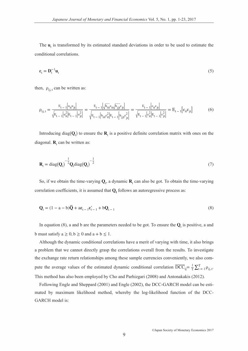
The ut is transformed by its estimated standard deviations in order to be used to estimate the

conditional correlations.

εt = Dt−1ut (5)

then, ρij, t can be written as:

ρij, t =Et − 1 uitujt

Et − 1 uit2 Et − 1 ujt

2=

Et − 1 hiitεit hjjtεjt

Et − 1 hiitεit2 Et − 1 hjjtεjt

2=

Et − 1 εitεjt

Et − 1 εit2 Et − 1 εjt

2= Et − 1 εitεjt (6)

Introducing diag Qt to ensure the Rt is a positive definite correlation matrix with ones on the

diagonal. Rt can be written as:

Rt = diag Qt− 1

2Qtdiag Qt− 1

2 (7)

So, if we obtain the time-varying Qt, a dynamic Rt can also be got. To obtain the time-varying

correlation coefficients, it is assumed that Qt follows an autoregressive process as:

Qt = 1 − a − b Q− + aεt − 1εt − 1′ + bQt − 1 (8)

In equation (8), a and b are the parameters needed to be got. To ensure the Qt is positive, a and

b must satisfy a ≥ 0, b ≥ 0 and a + b ≤ 1.

Although the dynamic conditional correlations have a merit of varying with time, it also brings

a problem that we cannot directly grasp the correlations overall from the results. To investigate

the exchange rate return relationships among these sample currencies conveniently, we also com-

pute the average values of the estimated dynamic conditional correlation DCCij=1T ∑t = 1

T ρij, t.

This method has also been employed by Cho and Parhizgari (2008) and Antonakakis (2012).

Following Engle and Sheppard (2001) and Engle (2002), the DCC-GARCH model can be esti-

mated by maximum likelihood method, whereby the log-likelihood function of the DCC-

GARCH model is:



L = − 12 ∑t = 1

T n*ln 2π + 2ln Dt +ut′Dt−1Dt

−1ut − εt′εt + ln Rt + εt′Rt−1εt (9)

equation (9) can be written as the sum of two parts: a volatility part and a correlation part.

L θ, φ = Lv θ + Lc θ, φ (10)

Lv θ is the volatility part:

Lv θ = − 12 ∑t = 1

T n*ln 2π + 2ln Dt +ut′Dt−1Dt

−1ut (11)

Lc θ, φ is the correlation part:

Lc θ, φ = − 12 ∑t = 1

T ln Rt + εt′Rt−1εt − εt′εt (12)

However, the assumption that εt follows a normal distribution is not always appropriate for

some financial data such as a daily exchange rate. Therefore, the multivariate student’s distribu-

tion is used in this paper (see Harvey, Ruiz and Shephard (1992) and Fiorentini, Sentana and Cal-

zolari (2003)). Jensen and Lunde (2001) consider that the results of the first part are virtually

unaffected by the change in error distribution, hence the first part is the same as equation (11).

Then the second part is:

Lc(θ,φ) = ∑t=1T ln Γ v + n

2 − ln Γ v2 − n

2ln π v − 2 − 12ln |Rt|

− v+n2 ln 1 +

u′tDt−1Rt

−1Dt−1ut

v − 2

(13)

Through equation (13), the parameters can be obtained when εt follows a t-distribution.

5. Estimation of dynamic conditional correlations

The DCC-GARCH (1, 1) model is estimated by the econometric software Oxmetrics 6. As

presented in Tables 3 and 4, β + γ < 1 and a + b < 1 hold for all the currencies both against the

NZD and USD. The dynamic conditional correlations between these currencies’ exchange rate

returns are shown from Figures 2 to 7. According to these figures, we can see the correlations



varies in time.

In Figure 1, the rate of USD/RMB reaches its valley bottom on January 14, 2014. If we chose

that day as the break point, the sample period can be divided into two sub-periods. The RMB

appreciated against the USD during the first period (period A); then depreciated during the sec-

ond period (period B). The RMB’s fluctuation also presented different features before and after

January of 2014. On March 17, 2014, just about two months after the beginning of the period B,

the PBC expanded the RMB’s de jure daily fluctuation band from 1% to 2%. As a result, the

RMB exchange rate was more flexible. For example, the average of RMB’s daily volatility (the

square of the exchange rate return) was 0.00000289 after January 14, 2014; while it was only

0.00000123 before that time.

The DCC-GARCH model allows us to compare the results of these two sub-samples before

and after the break point. Tables 3 and 4 displays the results and mean values of these DCC(s)

and DCC(s)* when we chose the NZD and USD as the numeraire currency respectively.

5.1 The USD’s status in East Asian exchange rate return co-movements

By introducing the NZD as the numeraire currency, the exchange rate returns correlations

between the USD and other currencies can be detected. In Table 3, for the RMB and EACs, the

exchange rate return co-movements with the USD were significantly larger than with the EUR

and JPY during both periods.6 This means that the East Asian currencies including the RMB

always keep closer relationship with the USD. This result coincides with some other researchers’

conclusions (for example, Kawai and Pontines (2014a; 2014b)) obtained by the FW model, in

which the USD occupied a highest weight in the currency baskets. Among these currencies, the

DCC of the KRW and USD was the lowest one which seldom exceeded 0.8. This result means

that the KRW is the “farthest” currency from the USD. This result coincides with reality that

Korea has a de jure floating exchange rate regime.

Comparing to the EACs, the RMB kept a much closer relationship with the USD in exchange

rate return which can be seen from the average values of the DCC(s) in Table 3. The

DCCUSD – RMB is the highest one among these average values, even higher than 0.98 during both

periods. Moreover, there are no significant differences in average value between the

DCCSGD – RMB and DCCSGD – USD, also DCCTHB – RMB and DCCTHB – USD during both periods.

These DCC(s) can also be intuitively observed through Figures 2 to 6 in which the lines of the

DCCEACs − RMB and DCCEACs − USD twist together most of the time. This consequent is due to a

very tight fluctuation range in the exchange rate of USD-RMB, both before and after January

2014. There is an unusual point in DCCUSD − RMB should be noticed. On August 11, 2015, the

PBC launched a violent exchange rate system reform; the exchange rate of RMB against the



Table 3. The mean values of the dynamic conditional correlations and means comparison (Numeraire currency: NZD)MYR

β 0.0241 [0.0000]*** γ 0.9693 [0.0000]***Average value of DCC Period A Period B comparison of mean tests(A)

DCCMYR–USD 0.8206 0.7666 25.9968***DCCMYR–RMB 0.8317 0.7828 24.7101***DCCMYR–EUR 0.5804 0.5352 13.8919***DCCMYR–JPY 0.5742 0.5257 11.2807***

comparison of mean tests (B) (-136.5372)*** (119.5809) ***comparison of mean tests (C) (6.5607) *** (6.6955) ***

SGDβ 0.0268 [0.0000]*** γ 0.9635 [0.0000]***

Average value of DCC Period A Period B comparison of mean testsDCCSGD–USD 0.8944 0.8852 (10.7974)***DCCSGD–RMB 0.8946 0.8857 (10.6049)***DCCSGD–EUR 0.7169 0.7283 (-4.9437)***DCCSGD–JPY 0.6992 0.7052 (-2.2551)**

comparison of mean tests (B) (161.0609) *** (129.4917) ***comparison of mean tests (C) (0.2589) (0.5878)

KRWβ 0.0260 [0.0000]*** γ =0.9650 [0.0000]***

Average value of DCC Period A Period B comparison of mean testsDCCKRW–USD 0.7467 0.6957 16.9557***DCCKRW–RMB 0.7549 0.7097 16.5104***DCCKRW–EUR 0.5551 0.5565 -0.4061DCCKRW–JPY 0.5115 0.5196 -1.8557*

comparison of mean tests (B) (132.7473) *** (-125.5242) ***comparison of mean tests (C) (-3.3046) *** (4.1894) ***

TWDβ 0.0297 [0.0000]*** γ 0.9608 [0.0000]***

Average value of DCC Period A Period B comparison of mean testsDCCTWD–USD 0.9332 0.9129 17.1274***DCCTWD–RMB 0.9331 0.9144 16.7364***DCCTWD–EUR 0.6654 0.6662 -0.2555DCCTWD–JPY 0.6814 0.6555 7.5036***

comparison of mean tests (B) (87.8460)*** (59.0473)***comparison of mean tests (C) (-0.1378) (1.0410)

THBβ 0.0291 [0.0000]*** γ 0.9607 [0.0000]***

Average value of DCC Period A Period B comparison of mean testsDCCTHB–USD 0.9121 0.9193 -5.2761***DCCTHB–RMB 0.9083 0.9090 -5.0736***DCCTHB–EUR 0.6680 0.6773 -3.9398***DCCTHB–JPY 0.6869 0.6853 0.4156

comparison of mean tests (B) (80.9914)*** (58.9191)***comparison of mean tests (C) (-2.7947) *** (-6.9854) ***

RMB DCCUSD–RMB 0.9888 0.9805 (23.4734) ***

a 0.0192 [0.0000]*** b 0.9664 [0.0000]***

Notes: β, γ, a and b are the parameters in equations (4) and (8), respectively. The table presents the t-test results for the null hypothesis: (A) the average DCC is the same before and after January 14, 2014; (B) the average DCC is the same for DCCUSD–RMB and DCCEACs–USD during the same period; (C) the average DCC is the same for DCCEACs–RMB and DCCEAC–USD during the same period. [ ] and ( ) denote p-values and t-values, respectively; ***, **, * represent significance at 1%, 5%, and 10% respectively. We also test the null hypothesis that DCCEACs–USD equals to DCCEACs–EUR and DCCEACs–JPY by t-test. All the p-value(s) are 0 suggesting that DCCEACs–USD ≠ DCCEACs–EUR; DCCEACs–USD ≠ DCCEACs–JPY.



USD decreased by 1.84% on that day and fluctuated in the next few days. As a result, the

DCCUSD − RMB sharply decreased during that time. However, it returned to high level gradually

after then.

After five exchange rate system reforms, the RMB exchange rate became more flexible to

Table 4. The mean values of the dynamic conditional correlations between the RMB and other East Asian currencies (Numeraire currency: USD)

MYRβ 0.0617 [0.0099] *** γ 0.9229 [0.0000]***

Average value of DCC Period A Period B comparison of mean tests(A)DCCMYR–RMB* 0.2926 0.2902 0.6395

SGDβ 0.0539[0.0000]*** γ 0.9433[0.0000]***

Average value of DCC Period A Period B comparison of mean testsDCCSGD–RMB* 0.2109 0.2501 -8.8253***

KRWβ 0.0487 [0.0000]*** γ 0.9467 [0.0000]***

Average value of DCC Period A Period B comparison of mean testsDCCKRW–RMB* 0.2255 0.2556 -7.0323***

TWDβ 0.0541 [0.0000]*** γ 0.9394 [0.0000]***

Average value of DCC Period A Period B comparison of mean testsDCCTWD–RMB* 0.2271 0.2888 -13.7345***

THBβ 0.0820 [0.0000]*** γ 0.8676 [0.0000]***

Average value of DCC Period A Period B comparison of mean testsDCCTHB–RMB* 0.1600 0.1652 -1.2400

a 0.0143 [0.0000]*** b 0.9755 [0.0000]***

Notes: β, γ, a and b are in equations (4) and (8), respectively. The table presents the t-test results for the null hypothesis: the average DCC is the same before and after January 14, 2014. [ ] and ( ) denote p-values and t-values, respectively; ***, **, * represent significance at 1%, 5%, and 10% respectively.

Figure 2. Dynamic conditional correlations between the MYR and other currencies (Numeraire currency: NZD)



some extent. However, the RMB has not radically extricated itself from the USD in terms of

exchange rate return, at least until September of 2016. In the “impossible trinity”, the Chinese

monetary authority may not give up the independence of its monetary policy. For the capital

account, its openness is based on the reform of China’s domestic financial sector which is a very

complicated project, and this reform has not been very successful (Volz, 2014). In this case, for

the risk-averse Chinese government, there is not sufficient motivation to promote capital account

liberalization. As a coin has two sides, the effect of RMB exchange rate system reform has not

been obvious.

Meanwhile, three (MYR, KRW and TWD) of the five EACs showed obviously lower average

DCC(s) with the USD during the second period suggesting that these currency have become

Figure 3. Dynamic conditional correlations between the SGD and other currencies, (Numeraire currency: NZD)

Figure 4. Dynamic conditional correlations between the KRW and other currencies, (Numeraire currency: NZD)



more significantly flexible in recent years. This result can also be observed from Figures 2, 4 and

5, the DCC(s) between these currencies and USD are presented as down-trend lines in the second

period.

For the EACs, the USD and RMB look like the same currency when we chose the NZD as the

numeraire currency. As a result, when these three currencies (MYR, KRW and TWD) got away

from the USD, they were also far away from the RMB in the long-run. In Table 3, all of the aver-

age DCC(s) between the RMB and EACs become lower during period B, except the THB. In this

view, the exchange rate return co-movement between the RMB and EACs had not been stronger

after the RMB shifted into depreciation trend.

Figure 5. Dynamic conditional correlations between the TWD and other currencies (Numeraire currency: NZD)

Figure 6. Dynamic conditional correlations between the THB and other currencies, (Numeraire currency: NZD)



5.2 The exchange rate return co-movements between the RMB and EACs, excluding the USD.

However, there is a different scence when we use the USD as the numeraire currency. Choos-

ing the USD as the numeraire currency is much nearer to reality, although this means that we

exclude the USD from the sample currencies and we are unable to detect the USD’s role in East

Asia from an outside perspective. The results are presented in Table 4, the DCC(s) are rewritten

as DCC(s)*. We also take the January 14, 2014 as a break-point. Figure 7 shows the evolution of

the DCC(s)* between the RMB and EACs.

In Table 4, three (SGD, KRW, TWD) of the EACs showed relatively higher average DCC(s)*

during the period B than during the period A. In other words, the exchange rate return co-

movements between the RMB and these three currencies became closer after the RMB turned

into a depreciation trend and became more flexible. By contrast, DCCMYR – RMB* and

DCCTHB – RMB* did not increase significantly during the period B.

Figure 7 intuitively shows the evolution of the DCCEACs − RMB(s)* when the RMB was in the

depreciation trend. August 11, 2015 is a meaningful point caught by the DCC-GARCH model.

When the RMB sharply fluctuated against the USD after the PBC launched a new exchange rate

system reform, the DCCEACs − RMB* also changed obviously in short-run. The increasing

DCCSGD − RMB*, DCCKRW − RMB

* and DCCTWD − RMB* mean that the exchange rate return co-

movements between the RMB and these three currencies were stronger when the RMB depreci-

ated and fluctuated against the USD suddenly. However, the MYR and THB were far away from

the RMB during those days. The DCCMYR − RMB* dropped from 0.24 to 0.09; the DCCTHB − RMB

*

decreased from 0.13 to 0.05. This unusual point is a short-run evidence that the co-movement of

Figure 7. Dynamic conditional correlations between the RMB and other currencies, (Numeraire currency: USD)



RMB-MYR and RMB-THB did not rise significantly when RMB devaluated to the USD acci-

dentally. The reality also supports these results. On August 11, 2015, the SGD, KRW and TWD

simultaneously depreciated against the USD by 1.5%, 1.7% and 1.7% when the RMB suddenly

depreciated. These fluctuations are very large for these currencies. On the other hand, the MYR

and THB were very stable, the exchange rate returns against the USD were almost 0.

5.3 Economic fundamentals of the increasing DCC(s)* between the RMB and EACs

We will investigate why some DCC(s)* became lager while others not when the RMB became

more flexible and depreciating during the period B. FDI and international trade are two represen-

tative factors for the economic relationship between two countries, therefore we discuss the issue

through these two ways.

According to the data released by Coordinated Portfolio Investment Survey (CPIS), Singa-

pore, Korea and Taiwan kept very close bilateral FDI relationship with China (Figure 8). Further-

more, China occupied first place in terms of these three countries’ bilateral FDI positions. For

Taiwan, more than 24% of bilateral FDI positions came from China during the years from 2010

to 2015. Singapore and Korea also kept higher than 10% FDI positions with China. In contrast,

the FDI relationships between China and Malaysia, as well as Thailand were relatively loose dur-

ing both periods. Malaysia kept the closest FDI relationship with Singapore. For Thailand, Japan

was always the most important country in terms of FDI. A stable bilateral exchange rate is help-

ful in stabilizing the FDI between these two countries. As a result, when the RMB became more

flexible in the depreciation trend, the exchange rate return co-movements with the RMB were

also tighter for Singapore, Korea and Taiwan.

Pontines and Sirega (2012) consider that the East and Southeast countries’ “fear of apprecia-

Figure 8. The bilateral FDI relationship between China and East Asian countries (region)

Data source: Coordinated Portfolio Investment Survey.



tion” against the RMB because they competed with China in the field of export. In this paper, we

will discuss this “fear” from another perspective: trade surplus with China. In Figure 9, more

than 100% trade surplus of Korea and Taiwan came from China in 2010. Although these ratios

dropped below 100% in 2015, they were still higher than 50%. In other words, China is the most

important market provider for Korea and Taiwan. On the other hand, Malaysia obtained little

trade surplus from China in 2010. Then this surplus turned into deficit in 2015. Thailand always

kept trade deficit with China. For a trade surplus country, the low value of its currency is an

effective way to keep this surplus. For the trade deficit countries, the opposite is true.

From the discussion above, we can conclude that the countries (region) who kept close FDI

relationship with China, the exchange rate return co-movements between their currencies and the

RMB were also closer during period B. Also, for Korea and Taiwan, who run large trade surplus

with China, the exchange rate return co-movements between their currencies and the RMB also

became larger when the RMB shifted into a depreciation trend. By comparison, the

DCCMYR − RMB* and DCCTHB − RMB

* were not significantly larger during the period B than dur-

ing period A, when Malaysia and Thailand kept loose FDI and trade relations with China.

Although the DCC-GARCH model cannot distinguish the official interventions from pure

market force, we can still discuss this issue from the perspective of exchange rate regime.

For the RMB, neither of the EACs is an important currency in the RMB’s currency basket. For

example, the PBC Governor Zhou Xiaochuan stated that the U.S. Dollar (USD), Euro (EUR) and

Japanese Yen (JPY) were the most important currencies in the RMB’s currency basket.7 In

December 2015, China Foreign Exchange Trading System & National Interbank Funding Center

(CFETS), which is a sub-institution of the PBC, introduced the CFETS RMB index. According

Figure 9. The sample East Asian countries’ (region) trade surplus with China

Data source: UN Comtrade; Customs Administration, Republic of China.



to the CFETS RMB index, the USD, EUR and JPY are the three most important currencies. As a

result, it is unlikely that the PBC actively adjust the exchange rate co-movements of RMB-

EACs.

For the EACs, the IMF classifies Korea (KRW) and Thailand (THB)’s exchange rate arrange-

ment as “floating”.8 Thus the official intervention is not the main force pushing the KRW close

to the RMB during period B. For the THB, because the FDI and trade relationships between

China and Thailand were relatively loose, neither the marketers nor the Thai authorities would

pay much attention to the co-movement between the RMB and THB.

Singapore has a “stabilized” exchange arrangement with a secretive composite anchor which

is established by Monetary Authority of Singapore. This currency basket is composed by their

major trading partners and competitors’ currencies, thus we consider the RMB is an important

currency in this basket because of the close trade relationship between these two countries.9 In

the short-run, the SGD exchange rate fluctuates freely within a target band. However, the cur-

rency basket is the center of the exchange rate in the long-run. The Center Bank of the Republic

of China (Taiwan) declares that “the TWD exchange rate is determined by the market. However,

when the market is disrupted by seasonal or irregular factors, the Bank will step in.”10 So, Tai-

wan’s exchange rate regime can be thought as a “management floating” arrangement. We deduce

that the co-movement of the SGD-RMB and TWD-RMB are forced by both marketers and

authorities. According to the IMF, Malaysia has an “other managed” exchange rate arrangement;

the Bank of Negara Malaysia (the central bank of Malaysia, BNM) declares they have a managed

floating exchange rate arrangement. This means that the MYR exchange rate is decided by both

pure market and authority. However, the relationship between the MYR and RMB seems to be

closer than it should be. The DCCMYR − RMB* is the highest DCC* during the both periods, as

high as about 0.29, although it increased insignificantly. Another noteworthy event is: when the

PBC pronounced that the RMB would no longer be pegged to the US dollar on July 21, 2005, the

BNM also announced the end of the MYR’s peg to the USD on the same day. Therefore, we con-

clude that the co-movement between the MYR and RMB is also forced by a mix force.

6. Conclusions

This paper has examined the dynamic conditional correlations among the sample currencies by

applying the DCC-GARCH model.

By choosing the NZD as the numeraire currency, we have fund that the USD was still the most

important currency in East Asia. However, its importance has been weakened as the DCC(s)

between the USD and EACs, except the THB, became less during recent years. This also sug-

gests that the exchange rates of these East Asian currencies became more flexible. Meanwhile,



the dynamic conditional correlation of the USD-RMB were very high (although it became lower

during the period B) during both periods due to RMB’s narrow fluctuation band against the USD.

This reflects the RMB exchange rate flexibility has increased slowly, comparing to other East

Asian currencies. We can conclude that China’s exchange rate system reforms were not very

effective. As a result, the exchange rate return co-movements between the EACs and RMB

became weaker during the second period. The EACs also departed from the RMB when they

attached less importance to the USD.

However, when we chose the USD as the numeraire currency, the exchange rate return co-

movements between the RMB and some of the EACs showed a rise during the second sub-

sample period. We have found that: when a country (region) kept close FDI and trade relations

(trade surplus) with China, their currencies also fluctuated nearly with the RMB after January

2014. These results confirm the existence of the “fear of appreciation and fluctuation” against the

RMB in SGD, KRW and TWD. By investigating the EACs’ exchange rate regimes, we consider

that Korea’s “fear” mainly came from pure market; Singapore and Taiwan’s “fear” came from

both marketers and authorities. For Thailand, neither the authority nor marketers “fear of appre-

ciation and fluctuation” against the RMB.

It seems the results are quite mixture even contradictory when we employ the NZD and USD

as the numeraire currency respectively. In fact, this just reveal the RMB’s increasing but limited

role in East Asia. On the one hand, the close economic relationships between China and some

countries was a fundamental for strong exchange rate co-movement, particularly, when the RMB

became more flexible and deprecating. On the other hand, the relatively slow pace of further

exchange rate system reform causes the RMB to be still near to the USD. Therefore, the RMB

had been neither a polar of East Asian exchange rate system nor a challenger to the USD, at least

until September 2016. If the RMB exchange rate system can be reformed further in the future,

the RMB could potentially attract more attention in East Asia.

NOTES

1) The sum of the percentage shares are 200% because two currencies are involved in each

transaction.

2) Data source: Currency Composition of Official Foreign Exchange Reserves, IMF.

3) See Subramanian and Kessler (2013); Henning (2012); Ho, Ma and McCauley (2005);

Balasubramaniam, Patnaki and Shah (2011); Kawai and Pontines (2014a, 2014b).

4) IMF: Annual Report on Exchange Arrangements and Exchange Restrictions 2014.

5) June 19 and 20, 2010 are weekend.



6) These means are also compared by t-test. All of the p-values are 0 demonstrates the means

are significantly different.

7) PBC: Speech of Governor Zhou Xiaochuan:

http://www.pbc.gov.cn/english/130724/2829809/index.html.

8) IMF: Annual Report on Exchange Arrangements and Exchange Restrictions 2014.

9) Some studies estimate the RMB’s weight in the SGD’s currency basket. For example,

Kawai and Pontines (2014a, 2014b) consider the weight occupied by the RMB is higher

than 0.2 after the year of 2010. Henning (2012) obtains the result of 0.364 during the period

between June, 2010 to December, 2011. The RMB’s weight is even higher than 0.49 in Sub-

ramanian and Kessler (2013)’s paper. Although these results are debatable, they can still

illustrate that the RMM is an important currency in the SGD’s currency basket.

10) Center Bank of the Republic of China (Taiwan):

http://www.cbc.gov.tw/ct.asp?xItem=856&CtNode=480&mp=2.

Acknowledgment

We thank professors Eiji Ogawa, Hisashi Nakamura and Kentaro Kawasaki for their helpful

advice. Of course, we are responsible for our own errors.

References:

Antonakakis, N. (2012). Exchange Return Co-movements and Volatility Spillovers Before and

After the Introduction of Euro. FIW Working Paper 80, May.

Balasubramaniam, V., Patnaik, I., & Shah, A. (2011). Who Cares About the Chinese Yuan?

NIPFP Working Paper No. 89. New Delhi: National Institute of Public Finance and Policy.

Bollerslev, T. (1990). Modelling the Coherence in Short-run Nominal Exchange Rates: A Multi-

variate Generalized ARCH model. Review of Economics and Statistics, 72: pp. 498–505.

Calvo, G. A., & Reinhart, C.M. (2002). Fear of Floating. The Quarterly Journal of Economics,

Vol. 117, No. 2, pp. 379–408.

Cho, J. H., & Parhizgari, A. M. (2008). East Asian Financial Contagion under DCC-GARCH.

International Journal of Banking and Finance, Vol. 6: Iss.1, Article 1.

Christodoulakis, G.A., & Satchell, S.E. (2002). Correlated ARCH: Modeling the Time-varying

Correlation between Financial Asset Returns. European Journal of Operations Research, 139:

pp. 351–370.

Colavecchio, R. & Funke, M. (2008). Volatility transmissions between renminbi and Asia-Pacific

on-shore and off-shore U.S. dollar futures. China Economic Review, 19: pp. 635–648.



Engle, R.F. (2002). Dynamic Conditional Correlation- A Simple Class of Multivariate GARCH

Models. Journal of Business and Economic Statistics, 20: pp. 339–350.

Engle, R.F., & Sheppard, K. (2001). Theoretical and Empirical Properties of Dynamic Condi-

tional Correlation Multivariate GARCH. Stern Finance Working Paper Series FIN-01-027

(Revised in Dec. 2001), New York University Stern School of Business.

Fiorentini, G., Sentana, G., & Calzolari, G. (2003). Maximum Likelihood Estimation and Infer-

ence in Multivariate Conditionally Heteroskedastic Dynamic Regression Models with Student

t Innovations.” Journal of Business and Economic Statistics, 21: pp. 532–546.

Frankel, J., & Wei, S. J. (1994). Yen Bloc or Dollar Bloc? Exchange Rate Policies of the East

Asian Economies. In T. Ito & A.O. Krueger (Eds.), Macroeconomic Linkages: Savings,

Exchange Rates and Capital Flows (pp. 295–333). Chicago: University of Chicago Press.

Harvey, A., Ruiz, E., & Shephard, N. (1992). Unobservable Component Time Series Models

with ARCH Disturbances. Journal of Econometrics, 52: pp. 129–158.

Henning, R. (2012). Choice and Coercion in East Asian Exchange Rate Regimes. Working Paper

Series 12–15. Washington Peterson Institute for International Economics.

Ho, C., Ma, G., & McCauley, R. (2005). Trading Asian Currencies. BIS Quarterly Review

(March): pp. 49–58.

Ito, T. (2010). China as Number One: How about the Renminbi? Asian Economic Policy Review,

5: pp. 249–276.

Jensen, M.B., & Lunde, A. (2001). The nig-s and arch model: A fat-tailed stochastic, and autore-

gressive conditional heteroscedastic volatility model. Working paper series No. 83, University

of Aarhus.

Kawai, M., & Pontines, V. (2014a). Is There Really a Renminbi Bloc in Asia? ADBI Working

Paper series, No. 467.

Kawai, M., & Pontines, V. (2014b). The Renminbi and Exchange Rate Regimes in East Asia.

ADBI Working Paper series, No. 484.

Keddad, B. (2016). How do the Renminbi and other East Asian currencies co-move? New evi-

dence from non-linear analysis? https://papers.ssrn.com/sol3/papers.cfm?abstract_id=2850421.

McKinnon, R., & Schnabl, G. (2004). The East Asian Dollar Standard Fear of Floating and Orig-

inal Sin. Review of Development Economics, 8: pp. 331–360.

Pontines, V., & Siregar, R.Y. (2012). Fear of appreciation in East and Southeast Asia: The role of

the Chinese renminbi. Journal of Asian Economics, 23: pp. 324–334.

Subramanian, A. & Kessler, M. (2013). The Renminbi Bloc Is Here: Asia Down, Rest of the

World to Go? Working Paper Series: WP-12-19. Washington Peterson Institute for Interna-

tional Economics.



Tse, Y.K., & Tsui, A.K.C. (2002). A Multivariate GARCH Model with Time-varying Correla-

tions. Journal of Business and Economic Statistics, 20: pp. 351–362.

Volz, U. (2014). RMB Internationalisation and Currency Cooperation in East Asia. in Rövekamp,

F., & and Hilpert (Eds.), Currency Cooperation in East Asia. Springer International Publishing,

Switzerland, pp. 57–81.



Documents

The exchange rate return co-movements between Renminbi and