The Evolution of the US Financial Industry from 1860 to2007: Theory and Evidence.∗

Thomas Philippon†

New York University, NBER, CEPR

November 2008

Abstract

The share of finance in U.S. GDP displays large historical variations. I argue, usingevidence and theory, that corporate finance is a key factor behind these evolutions.Corporate demand for intermediation depends crucially on the relative investment op-portunities of firms with low cash flows (young firms) and firms with high cash flows(incumbents). A simple general equilibrium model is developed in order to separatedemand and supply factors in the market for financial intermediation. The demandparameters accord well with historical evidence on the importance of entrants duringtechnological revolutions. The supply parameters suggest financial regress in the 1930sand progress in the 1990s. The model accounts for much of the variation in the incomeshare of the financial sector from 1860 to 2001. Only the period 2002-2007 appearspuzzling.

Keywords: Financial development, corporate finance, financial intermediation, func-tional analysis, moral hazard, structural change.JEL: E2, O16, G2, G3

∗I thank seminar participants at NYU, Duke, Toulouse, the Society for Economic Dynamics and theNBER for their comments.

†Stern School of Business, 44 West Fourth Street, Suite 9-190, New York, NY 10012-1126. Tel: +1 212998 0490, tphilipp@stern.nyu.edu.

1

Financial institutions provide services to households and corporations. The financial

sector’s share of aggregate income reveals the value that the rest of the economy attaches

to these services. Historical data from the United States shows surprisingly large variations

in the economic importance of Finance. It was high in the 1920s, but, after a continuous

collapse in the 1930s and 40s, it was down to only 2.5% of GDP in 1947. It recovered slowly

until the late 1970s, and then grew more quickly to reach almost 8% of GDP in 2006.

The interactions between Finance and the rest of the economy are complex. Economic

growth in the 1960s was outstanding, but seemed to require little financial intermediation.

Finance grew quickly in the 1980s while the economy stagnated, and the pattern changed

again in the 1990s. These evolutions could offer valuable insights into the process of eco-

nomic growth, but they have received little attention so far.

The finance industry, unlike other sectors, would not exist in an Arrow-Debreu economy.

If markets were complete, financing and insuring would be trivial. How then should we

interpret the dramatic growth of this industry over the past 60 years? Does this imply that

the U.S. economy has drifted away from the Arrow-Debreu benchmark? Is information

becoming more asymmetric, or enforcement more difficult? Why is the U.S. devoting a

growing share of its human capital to the provision of financial services? Which economic

forces pin down the equilibrium size of the financial sector? This paper attempts to answer

these questions by bringing together new evidence and theory.

The paper focuses on the role of corporate finance, because the evidence suggests that

other explanations for the evolution of the financial sector are either incorrect or incomplete.

Contrary to common wisdom, there is neither theoretical nor empirical support for the idea

that total factor productivity (TFP) growth in the non financial sector has a direct influence

on the size of the financial sector. Neither financial globalization, nor increased trading of

securities, nor the development of the mutual funds industry can account for the increasing

share of finance in GDP. Moreover, the usual explanations given for the increasing share of

the service sector in the economy do not apply to the finance industry.

To further motivate the focus on corporate finance, I present new evidence on the evo-

lution of the cross-sectional distribution of cash flows and investment expenditures. I find

that firms with low cash flows account for a growing share of total capital expenditures.

In the 1950s, most corporate investment was done by incumbents with high cash flows.

2

In 2000, half of total investment was done by (young) firms whose cash flows covered less

than a third of their capital expenditures. What we observe, however, is the distribution

of cash flows and realized investments, and not the distribution of investment opportuni-

ties. This evolution might reflect either increasing demand for financial intermediation, or

improvements in financial intermediation (supply shocks), or both.

An equilibrium model of intermediation is therefore needed to interpret the evidence.

Greenwood and Jovanovic (1990) and Bencivenga and Smith (1991) are important references

in the literature. These models, however, are not sufficient to address the issues raised by

the empirical evidence. Models with exogenous fixed costs of trading do not provide an

interpretation for the link between investment and cash flows, which is the cornerstone

of corporate finance. In addition, models based on trading costs are unlikely to explain

the growth of the finance industry since, as Freixas and Rochet (1997) argue, “the progress

experienced recently in telecommunications and computers implies that FIs would be bound

to disappear if another, more fundamental, form of transaction costs were not present.” In

the model of Bencivenga and Smith (1991), it is possible to study the balance sheet of

financial intermediaries, but not their value added since the modelled intermediaries do not

have employees.1

The model economy is populated by overlapping generations of agents who choose to

work in the financial or in the non-financial sector. Following Diamond (1984) and Holm-

ström and Tirole (1997), among others, I focus on corporate finance and monitoring in the

presence of moral hazard. Agents in the non-financial sector have different productivities

and receive different investment opportunities. Moral hazard limits borrowing, and agents

with good opportunities but low cash flows cannot always invest. Agents in the financial

sector help alleviate these borrowing constraints. In equilibrium, the market for corporate

financial services must clear, and young agents must be indifferent between careers in the

financial and non-financial sectors.

The model clarifies the economic forces that pin down the size of the financial sector.

First of all, the Finance share of income is constant along a balanced growth path: the

level of productivity in the non financial sector does not influence the size of the financial

1To be empirically useful, the model must also allow for both direct and intermediated finance. Bencivengaand Smith (1991) assume that all savings are intermediated.

3

sector. Under some conditions, this also applies to the rate of productivity growth, and this

is consistent with the historical evidence.

On the supply side, efficiency gains in finance always reduce credit rationing, but have

ambiguous effects on the relative size of Finance. When the financial sector is inefficient,

efficiency gains increase its income share, but when the sector is already quite efficient,

further gains reduce its income share. As a result, the size of the financial sector is not a

straightforward measure of market incompleteness, although it does contain useful informa-

tion.

On the demand side, there is an important distinction between moral hazard at the

micro level, and the relevant measure of moral hazard at the macro level. At the macro level,

the joint distribution of current productivity and investment opportunities is a fundamental

determinant of the aggregate demand for financial services. The intuition is that, when firms

with investment opportunities also receive high cash flows, there is little macro demand for

intermediation, even if moral hazard is potentially severe at the micro level. Finance is

more needed when young firms or young industries have better investment opportunities

than large established firms or industries. This prediction receives strong empirical support.

To go deeper into the analysis of the financial sector, the technological parameters of the

model are estimated by matching empirical moments. The model is then used to study the

historical data. The model quantifies the efficiency of the financial sector in each period,

and recovers the distribution of productivities and investment opportunities.

The model-implied structural parameters shed light on the evolution of the US economy

over the past 150 years. The 1890s and 1920s are a time a rapid entry and investment

by firms with large financial needs. These needs decrease during the two World Wars. A

structural shift happens during World War 2. After the War, large established firms with

high cash flows appear to have the best investment projects. As a result, the demand

for financial intermediation is small. Starting in the 1970s, investment opportunities shift

away from large profitable firms towards young firms with low current cash flows, and the

demand for intermediation increases. These predictions of the model are consistent with the

historical evidence on General Purpose Technologies, the role of Electrification in the 1920s

and Information Technology starting in the 1970s (David (1990), Jovanovic and Rousseau

(2005)).

4

On the supply side of financial services, the 1930s represent a financial disaster. The

efficiency of the financial sector collapses and a large number of firms become credit con-

strained. Efficiency in finance recovers after the War but remains below its level of the

1920s for three decades. In the 1980s the financial sector is not efficient enough to meet

the demands of the corporate sector and credit constraints rise in the 1980s. In the 1990s,

financial efficiency improves and leads to an investment boom.

The model can further be tested by considering its predictions for the income share of

(corporate) finance and for the size of the corporate credit market. The income share of

finance is nothing more that a broad-based measure of the fees, spreads, and other income

paid by the non-financial sector to the financial sector. The model correctly predicts much

of the variations in the income share of finance over more than 150 years. The model also

accounts reasonably well for the evolution of the credit market.

This paper is a first attempt to understand, qualitatively and quantitatively, the evo-

lution of the Finance industry in the US economy. In doing so, the paper makes several

empirical and theoretical contributions. The paper develops a new model of the equilibrium

size of the Finance industry that incorporates moral hazard, firm heterogeneity, monitoring

and career choices. The paper also presents new evidence for the U.S., at the industry level,

at the firm level, and at the individual level (regarding the tasks performed by employees

in the financial sector).

The paper is related to the literature on financial intermediation, reviewed in Gorton and

Winton (2003), and to the literature on financial development: King and Levine (1993), Do

and Levchenko (2007) and Greenwood, Sanchez, and Wang (2007) among others. Do and

Levchenko (2007), in particular, find that financial development responds to the demand

for external finance generated by international trade. In this paper, I estimate how the

financial sector responds to the demand for external finance generated by changes in the

distribution of investment opportunities.

The remaining of the paper is organized as follows. Section 1 presents the evidence and

discusses alternate explanations. Section 2 presents the model and Section 3 characterizes

the equilibrium allocations. Section 4 estimates the parameters of the model. Section 5

tests the prediction of the model using historical data. Section 6 concludes.

5

1 Evidence

This section describes the evolution of the U.S. financial sector. Its goal is to present the

facts that the theory must explain, but also to clarify a number of widespread misconceptions

regarding the financial sector and its evolution.

Value added and compensation shares

Figure 1 displays the share of the Finance and Insurance industry in the GDP of the

United States, estimated from 1850 to 2007. For the period 1947-2007, I use value added

measures from the Annual Industry Accounts of the United States, published by the Bureau

of Economic Analysis (BEA). For 1929-1947, I use the share of employee compensation

because value added measures are either unavailable or unreliable. I extend the series using

data from Kuznets (1941) and Martin (1939) for the period 1900-1929. For 1850-1900, I use

the Historical Statistics of the United States2, and Census data. The data are described in

Philippon and Reshef (2007).

The growth of the U.S. financial sector is the story of three waves and two crashes (the

2008 crash is not yet visible in the data). The financial industry was around 1.5% of GDP

in the mid-19th century. The first large increase between 1880 to 1900 corresponds to the

financing of railroads and early heavy industries.

The second big increase between 1918 and 1933 corresponds to the financing of the Elec-

tricity revolution, as well as automobile and pharmaceutical companies. General Electric

did its IPO in 1913, General Motors in 1920 and Procter & Gamble in 1932. Key discover-

ies of the 1920s and 1930s, such as insulin and penicillin, became mass-manufactured and

distributed.

After a continuous collapse in the 1930s and 40s, the GDP share of finance and insurance

industries was down to only 2.5% of GDP in 1947. It recovered after the war and was

mostly stable at around 4% until the late 1970s. The third large increase, from 1980 to

2001, corresponds to the financing of the IT revolution. The financial industry accounted

for 8.3% of GDP in 2006.

Figure 2 shows the evolution of the shares of various subsectors (starting in 1977 because

of data limitations). In the National Income and Product Accounts (NIPA), the finance in-

2Carter, Gartner, Haines, Olmstead, Sutch, and Wright (2006).

6

dustry is split into 4 categories: (i) Credit intermediation; (ii) Investment banking, venture

capital, brokerage, and portfolio management; (iii) Insurance and reinsurance; (iv) Pension

funds, mutual funds (open- and closed-end), and trusts. Figure 2 shows that credit inter-

mediation is the dominant activity, and, together with investment banking and brokerage,

the fastest growing. Funds and trusts account for a negligible share of value added. This

brings up two important issues: the distinction between assets and value added, and the

classification of the various activities in a theoretical model.

Value added versus assets under management

Figure 3 shows the allocations of value added and assets within the financial sector in 2005.

The data on value added is from the NIPA, as described above. The data on assets is from

the Flow of Funds Accounts. To create Figure 3, I have mapped the Flow of Funds into the

NIPA classification. Figure 3 makes it clear that there is no simple relationship between

value added and assets under management. As a result, the common wisdom that the rise

of the pension and mutual funds industry is the main factor behind the evolution of finance

severely misses the point. In fact, from a theoretical perspective, funds and trusts resemble

the Arrow-Debreu benchmark: they control a lot of assets without using much economic

resources.

To understand the growth of the financial sector, one should not focus on mutual funds,

but rather on credit intermediaries, investment banks and private equity. From a theo-

retical perspective, it means that models based purely on trading costs are unlikely to be

useful. Similarly, it is probably more important to explain value added than assets under

management.

Functional analysis

From a theoretical perspective, industry classifications are useful only to the extent that

they can be mapped into economic functions, as advocated by Merton (1995). To do so, one

must look at the tasks performed by employees of the financial sector. Figure 4 presents

estimates of the share of finance activity that is presumably related to corporate finance

and credit intermediation. The data is from Philippon and Reshef (2007) and the primary

source is the Current Population Survey. The estimates are based on the compensation of

7

employees, i.e., on employment weighted by relative wages.3

The baseline share is constructed by removing the jobs that are not related to corpo-

rate finance or to credit intermediation. The excluded categories are: insurance specialists;

traders of stocks, bonds, commodities and other assets; personal financial advisors; janitors,

private security and miscellaneous employees. The baseline share is one minus the compen-

sation share of the excluded categories. Figure 4 shows that the baseline share is relatively

stable, around 75%. This measure might overestimate corporate finance services, however,

because it includes all clerical and administrative jobs. Some of these workers keep track

of loans to businesses, but some also provide services to households. I therefore compute

a second estimate that excludes all clerks and administrative workers. This adjusted share

increases over time because of the decrease in clerical employment. Based on Figure 4, I

will assume that approximately 60% of finance activity is related to corporate finance, and

that this share has not declined over time.

Globalization

Globalization does not account for the growth of the U.S. financial sector, for two reasons.

First, the U.S., unlike the U.K., is not a large exporter of financial services. According

to IMF statistics, in 2004, the U.K. financial services trade balance was +$37.4 billions

while the U.S. balance was -$2.3 billions: the U.S. was actually a net importer. In 2005,

the U.K. balance was +$34.9 billions, and the U.S. balance was +$1.1 billions.4 Second,

financial globalization is a relatively recent phenomenon (see Obstfeld and Taylor (2002),

and Bekaert, Harvey, and Lumsdaine (2002)), while Figure 1 shows that the growth of the

financial sector has been continuous since the end of World War II.

Finance versus other industries

Is finance different from other service industries? Yes. The other fast growing service

industry is health care, but it does not share the U-shaped evolution of Finance from 1927

to 2006. In theory, Finance is clearly different because it would not exist in a Arrow-Debreu

economy, while almost all other services would. This fact has important implications that

3Weighting is important because wages vary with occupations. For instance, traders earn more thanclerks.

4There is, of course, much trade within the financial sector, notably between the U.S. and the U.K., butit would be misleading to argue that growth in value added of the U.S. finance and insurance industry isdue to large net exports.

8

are not well understood. In particular, it renders much of the literature on structural

change irrelevant for understanding of the evolution of the financial sector. The traditional

explanations for the growth of the service sector focus on the elasticity of substitution

between goods and services, and on rapid productivity growth in manufacturing (Baumol

(1967)). These ideas cannot be applied to the financial sector, for at least two reasons.

First, financial services do not enter directly into the utility function of agents; they enter

the budget constraint. As a result, there is no elasticity of substitution to speak of.5

The second reason why the usual models of structural change do not apply to Finance is

that the economic value added of one unit of financial services grows with the productivity

of the agents who benefit from these services.6 As a result, the equilibrium size of the

financial sector is independent of productivity in the non financial sector. In an earlier

version of this paper, I showed that productivity growth is indeed uncorrelated with the

size of the financial sector. The 1960s was the period of fastest productivity growth but it

was also the period where the financial sector remained essentially unchanged. The growth

of finance was strong in the 1980s, a time of low productivity growth. In the 1990s, however,

productivity and finance grew together. Productivity growth by itself does not account for

the evolution of the financial sector.

Investment share of low cash firms

The evidence just discussed suggests that neither the development of mutual and pension

funds, nor globalization, nor the traditional explanations for the rise of the service sector

can account for the evolution of the Finance industry. Some periods of economic growth

appear to be more intensive in finance than others, but, until now, we simply do not know

why.

5One can of couse imagine a reduced form model with ‘financial services in the utility function,’ just assome monetary models use ‘money in the utility function’ as a shortcut. But these reduced forms modelcannot be used to study the evolution of the financial sector for the same reasons one would not use ‘moneyin the utility function’ to study the structural determinants of transaction costs and money demand.

6When the utility function depends on real quantities of goods and services, it is conceptually (if notalways empirically) straightforward to define the relative productivity of various sectors. This is not thecase with financial services. To take a simple example, suppose that screening and monitoring services byone banker allow one entrepreneur to obtain financing. What is the productivity of the banker? The answeris that it is proportional to the productivity of the entrepreneur. In this simple example, the efficiency offinance is defined in terms of the number of entrepreneurs that a banker can screen, monitor and advise.This is the most natural way to think about corporate finance, and it implies that, for a given efficiency ofscreening and monitoring, productivity in finance grows with productivity in the non-financial sector. Thisproperty holds in the particular model developed below.

9

Figures 2 and 4 highlight the role of credit intermediation and corporate finance. What

is needed now is to look at the non financial sector in order to understand how financial

services are used. Corporate finance is fundamentally related to investment and internal

funds. Firms with low cash flows and high capital expenditures must raise external finance,

and they require financial services to do so. Empirically, I compute the share of investment

done by firms whose cash flows are less than a fraction α of their capital expenditures:

st =

Xi

capexit × (incomeit < α× capexit)Xi

capexit. (1)

I use all firms in the industrial Compustat files with non missing values for income and

capital expenditures, excluding finance, insurance and real estate. In equation (1), i is

the firm identifier, income is income before extraordinary items (Data #18), and capex is

capital expenditures (Data #128). To avoid issues with the timing of income and investment

— because of time-to-build or accounting rules — capexit and incomeit are the sum of capital

expenditures and income in year t− 2, t− 1 and t.

Figure 5 displays the shares of investment accounted for by low cash firms, defined

using three different cutoff values: α = 0.33, 0.25 and 0.15. All three measures show strong

upward trends. The investment share of low cash firms and the size of the corporate credit

market before 1940, presented in Table 1, are indirect estimates whose construction will be

discussed later.

Let me discuss briefly the issue of sample section and composition effects. First of all,

the coverage of Compustat in terms of capital expenditures and employment has remained

constant since 1975.7 Since the fastest growth in s33 happens after 1975, increased coverage

cannot explain the trend. Moreover, the increasing investment share of low cash firms

mostly reflects the fact that firms have been going public at a younger age over the past

50 years. Far from being a statistical sample bias, this is the consequence of financial

and technological innovations, and it is in fact evidence in support of the model presented

below.8

7The ratio of employees of all Compustat firms to Non Farm Payrolls is around 40%. The ratio of capitalexpenditures to non residential fixed investment is around 80%. These ratios are fairly constant from 1975to 2006.

8See Davis, Haltiwanger, Jarmin, and Miranda (2006) and Fink, Fink, Grullon, and Weston (2005) for

10

Interpreting the evidence

The evidence in Figure 5 is consistent with increasing demand for corporate finance ser-

vices, but it might also reflect improvements in financial intermediation, i.e., a supply shift.

Evaluating the respective contributions of supply and demand is critical in order to un-

derstand the evolution of the economy. For instance, demand and supply shocks in the

market for corporate finance are likely to have opposite implications for equilibrium credit

rationing and aggregate investment. A model is needed to understand the contributions of

supply and demand, and their connections to other characteristics of the economy, such as

the amount of outstanding corporate liabilities, and aggregate investment itself. The next

section presents a simple equilibrium model of corporate finance that can help us interpret

the evidence.

2 Model

Consider an infinite horizon production economy with overlapping generations of agents who

live for two periods. The economy has two sectors, industrial and financial. The industrial

sector produces a good that can be consumed and invested. The financial sector produces

monitoring services that are used by entrepreneurs of the industrial sector.

2.1 Technology and preferences

Agents discount the future at rate ρ and the size of each generation is normalized to 1. An

agent i ∈ [0, 1] born at time t consumes Ci1,t when she is young and C

i2,t+1 when she is old.

9

The agent chooses a career and a consumption path in order to maximize her expected

utility:

U it = Et

"Ci1,t +

Ci2,t+1

1 + ρ

#. (2)

Career Choice

In their first period, agents choose a career. Let nt be the mass of agents who choose the

industrial sector. The remaining 1− nt enter the financial sector. I start by describing an

evidence. Philippon and Sannikov (2007) show in a dynamic agency model that improvements in financialintermediation (especially in the VC industry) lead to a decline in the age of IPO firms.

9 In the description of the model, upper case letters denote variables that follow an upward trend becauseof technological progress. I later use lower case letters for the detrended variables.

11

agent’s career within the industrial sector. LetXt be a measure of the aggregate productivity

of the industrial sector at time t. After she enters the industrial sector, an agent receives

two random endowments: α ∈ (0,∞) and θ ∈ {0, θ}. Both α and θ are publicly observable.The first shock, α, determines the relative productivity of the agent in the first period of

her life. An agent i ∈ [0, nt] who receives a shock αi produces αiXt units of output. Let α

be the unconditional mean of α:

α ≡ E [α] . (3)

The second shock, θ, measures the investment opportunity of the agent. Investment requires

Xt units of output at time t and delivers θXt units of capital at time t + 1. Each unit of

capital is a Lucas tree that delivers one unit of consumption good per period and depreciates

at rate δ. Let π be the probability of receiving an investment opportunity:

π ≡ Pr³θ = θ

´. (4)

The shocks α and θ are correlated. Let F θ (.) be the cumulative distribution function of α

conditional on θ = θ, and let fθ (.) be the corresponding density function. The distribution

of α conditional on θ = 0 does not need to be specified explicitly.

Production and capital accumulation

Let Kt be the stock of capital (Lucas trees) at time t. Using equation (3), industrial output

is:

Yt = αntXt +Kt. (5)

This functional form is discussed later, with the other assumptions of the model. Capital

accumulates over time according to:

Kt+1 = (1− δ)Kt + θetXt, (6)

where et is the number of entrepreneurs. Given the definition of π in equation (4), we must

have:

et ∈ [0, πnt] . (7)

Moral hazard and monitoring

After investing Xt unit at time t, an entrepreneur can steal zXt units of capital at time

t + 1, while the remaining θXt − zXt is lost. The ratio z/θ captures the severity of the

12

moral hazard problem. Monitoring can be used to limit stealing. If mit units of monitoring

are allocated to entrepreneur i ∈ [0, et], she can steal only¡z −mi

t

¢Xt. Each agent in the

financial sector produces μ units of monitoring.

2.2 Markets

Market clearing

Let C1,t be the total consumption of the young agents, and let C2,t be the total consumption

of the old agents. Note that C1,t and C2,t are aggregate quantities and that agents within a

generation typically have different levels of consumption. Equilibrium in the goods market

requires:

C1,t + C2,t + etXt = Kt + αntXt. (8)

Equilibrium in financial intermediation requires:Zi∈[0,et]

mitdi = μ (1− nt) . (9)

The left hand side of equation (9) is the demand for monitoring services coming from all the

entrepreneurs active at time t. The right hand side is the aggregate supply of monitoring

by the 1− nt agents who work in the financial sector.

Asset prices

Let rt be the interest rate between period t and t+ 1. The ex-dividend price of one unit of

installed capital satisfies the dynamic equation:

qt =1 + (1− δ) qt+1

1 + rt. (10)

The net present value of a project is vtXt, where:

vt = θqt − 1. (11)

The interesting case is when projects are valuable, so the following assumption is maintained

throughout the paper:

Maintained assumption: θ > ρ+ δ

13

2.3 Discussion of the model’s assumptions

The model is meant to capture the financial services provided to the corporate sector. The

model abstracts from transaction and insurance services provided to households.10 To be

consistent, the model is calibrated to the share of finance that is related to corporate finance,

following the methodology used in Figure 4. Modeling financial intermediaries as monitors

follows a long tradition in economics and finance (see Diamond (1984) and Holmström

and Tirole (1997) for example). The main simplification is that the model assumes no

asymmetric information or moral hazard between savers and financial intermediaries. The

issue of ‘who monitors the monitors’ therefore does not arise, and only the productivity μ

matters for the equilibrium allocations.11

The important assumptions for the production function in equation (5) are constant

returns to scale and labor augmenting technology. It is well known that these are needed

for balanced growth. Scale must be indexed by Xt since the initial spending is measured

in units of output. Another possibility would be to specify that a project requires a fixed

number of man-hours. This would index project cost on wages, and therefore indirectly on

Xt. This would not change the general properties of the model. The fact that K and n

are perfect substitutes is only a simplification to reduce the dimension of the system and

allow a simple analysis of heterogeneity among entrepreneurs. Similarly, the assumption of

exogenous technological progress is convenient for the positive analysis presented here, but

is not critical.12

Finally, the model assumes a closed economy. This means that the entire demand for

financial services comes from domestic firms. Section 1 explains why this is a natural

benchmark, and Section 5 reconsiders the issue in light of the quantitative results.

10Levine (2005) defines five broad functions for the financial sector: screening, monitoring, trading, poolingof savings, and easing the exchange of goods and services. A model where the financial sector selects andcertifies projects has similar equilibrium implications as the model presented here.11Of course, these allocations can be decentralized with households buying some securities directly from

corporations and depositing the rest of their savings with financial intermediaries. Many equivalent imple-mentations are possible and, in the interest of space, they are not discussed here.12 It is conceptually straightforward to relax these assumptions: Philippon (2007), for instance, presents a

normative analysis in an endogenous growth model with a standard Cobb-Douglas production function.

14

3 Financial services in equilibrium

The definition of an equilibrium is standard. Agents maximize (2) by choosing a career

and a consumption path. Potential entrepreneurs choose whether to invest or not, and all

markets clear.

3.1 Balanced growth

Aggregate productivity Xt grows at rate γ: Xt+1 = (1 + γ)Xt. I use lower-case letters to

denote the quantities scaled by productivity: kt ≡ Kt/Xt, ct ≡ Ct/Xt, and so on. The scaled

quantities are constant on the balanced growth path. The interest rate is also constant.

Equation (6) implies k = θe/ (γ + δ), and equation (10) implies q = 1/ (r + δ). Equation

(11) becomes:

v =θ

r + δ− 1.

Combining the market clearing condition (8) with the budget constraint of old agents c2 =

k + (1− δ) qk, we obtain the investment/saving equation:

c1 = αn− ϕ (r) e, (12)

where the function ϕ (r) is defined by:

ϕ (r) ≡ 1 + 1− δ

r + δ

θ

γ + δ. (13)

I now describe the balanced growth of three economies. I quickly discuss the economy

without moral hazard, and the economy with moral hazard but without intermediation.

The model is simple enough that these cases can be understood directly by looking at

Figures 6 and 7. I then characterize the equilibrium with moral hazard and intermediation,

which is the main focus of the paper.

Consider first the case where z = 0. Projects are funded if and only v = θ/ (r + δ)− 1is positive. There are no financiers, and n = 1. The demand for entrepreneurship is:

ed (r) :

⎧⎨⎩= π if r + δ < θ∈ [0, π] if r + δ = θ= 0 if r + δ > θ

⎫⎬⎭ (14)

From equation (12) and the constraint that c1 be positive, we get:

es (r) :

⎧⎨⎩= 0 if r < ρ

∈ [0, α/ϕ (ρ)] if r = ρ= α/ϕ (r) if r > ρ

⎫⎬⎭ (15)

15

The equilibrium condition es (r) = ed (r) pins down the interest rate. The following propo-

sition characterizes the equilibrium, which is also depicted on Figure 6:

Lemma 1 Economy without moral hazard. When (1 + γ)π ≤ (δ + γ) α, all projects are

financed and e = π. Otherwise r = θ − δ, and e < π.

One important feature of this economy is that the equilibrium is independent of the condi-

tional distribution of productivity F θ (.). Only the unconditional mean α matters.

In this simple economy, the interest rate is constant at r = ρ as long as consumption

is interior, c1 > 0. Inspection of equation (12) shows that this is indeed the case if the

following condition holds:

Condition 1: α > πϕ (ρ).

3.2 Moral hazard without monitoring

Consider now the case where z > 0, but μ = 0. An entrepreneur borrows b when she is

young and produces θ units of capital when she is old.13 The cum-dividend value of one unit

of capital is (1 + r) / (r + δ). If the entrepreneur defaults, she gets z (1 + r) / (r + δ). If she

does not default, she gets (1 + r) θ/ (r + δ)− b (1 + r). The maximum amount of borrowing

allowed is therefore bmax = (θ − z) / (r + δ). An entrepreneur with current income α can

finance her investment if and only if α+ bmax > 1. This defines a threshold αh for financing

without monitoring:

1− αh (r) ≡ θ − z

r + δ. (16)

Internal cash must cover the difference between the pledgeable value of the project and the

capital expenditures required to start the project. Entrepreneurs whose income is less that

αh are financially constrained.

Let ec (r) be the effective investment demand curve under moral hazard. When r+δ > θ,

it collapses to zero, just like in equation (14). When r + δ ≤ θ, the constrained investment

demand is given by:

ec (r) = π³1− F θ [αh (r)]

´. (17)

13Recall that all these quantities are scaled by Xt.

16

When r + δ = θ, the effective demand curve is vertical and ec can be anywhere between

0 and π¡1− F θ

¡zθ

¢¢. The saving equation (15) is the same as in the economy without

moral hazard. The equilibrium is depicted on Figure 7 and characterized by the following

proposition:

Lemma 2 Economy without monitoring. Under condition 1, the interest rate is ρ and the

number of projects financed is ec (ρ).

Proof. Under assumption 1, equation (12) shows that c1 > 0. Therefore r = ρ.

Investment is pinned down by the constrained demand schedule ec evaluated at r = ρ.

3.3 Active intermediation

Consider now the case where z > 0 and μ > 0. An entrepreneur with current income α

hires m units of monitoring. The pledgeable income becomes (θ − z +m) / (r + δ). The

amount of monitoring required for this entrepreneur to be able to invest is:

m (α) = (r + δ) (αh − α) . (18)

Let φ be the price of one unit of monitoring. The NPV of a project, net of intermediation

costs, is v −mφ. It is profitable to use monitoring if α is more than αl, defined by:

m(αl)φ ≡ v. (19)

Let us now turn to the supply of financial services. Agents choose their careers freely,

therefore, in any equilibrium with intermediation, we must have:

μφ = α+ π³1− F θ (αh)

´v + π

Z αh

αl

(v − φm (α)) dF θ (α) . (20)

The left-hand-side of equation (20) is the value of entering the financial sector. The right-

hand-side is the value of entering the non-financial sector, which contains three terms: the

expected income from production, the expected value of becoming an entrepreneur who

can finance herself directly, and the expected value of becoming an entrepreneur who hires

financial services. Combining (19) and (20), I obtain:

μ

π=³ α

πv+ 1− F θ(αl)

´m(αl)−

Z αh

αl

m (α) dF θ (α) . (21)

17

Finally, equilibrium in the monitoring market requires that:

μ (1− n) = πn

Z αh

αl

m (α) dF θ (α) . (22)

Figure 8 describes the monitoring equilibrium. The balanced growth path with active

monitoring is characterized by αl and n that solve equations (21) and (22), and either r = ρ

or c1 = 0.

Lemma 3 Credit rationing persists as long as αl > 0, and the size of the financial sector

is strictly positive as long as fθ (αh) > 0.

Proof. The RHS of equation (21) goes to zero as αl → αh so for any value of μ > 0, it

is possible to find αl < αh that solves equation (21). If the density fθ (αh) > 0 and if fθ is

continuous, then the RHS of (22) is strictly positive and n is strictly less than one. QED.

The intuition for the lemma is the following. The price of monitoring φ is large when μ

is small, but entrepreneurs who are close enough to the cutoff αh are always willing to buy

the small amount of monitoring required to obtain financing.

Proposition 1 Equilibrium financial intermediation.

• The income share of the financial sector is constant on the balanced growth path.

• For a given interest rate, the income share of finance is independent of the growth rateof the economy. This is true in particular under condition 1.

• The size of the financial sector goes to zero when its efficiency becomes either verysmall or very large.

• Efficiency gains in finance reduce rationing and increase investment, but have anambiguous effect on the GDP share of the finance industry.

Proof. Equations (21) and (22) are independent of X, and of γ for a given value of r.

Under condition 1, equation (12) shows that c1 > 0. Therefore r = ρ. When r = ρ and the

share of finance is independent γ. The last two bullet points are proven in the appendix.

18

The first bullet point simply formalizes the intuition presented in section 1. The second

bullet point is fully consistent with the historical evidence.

The third bullet point makes clear that the model converges to two simple benchmarks

for extreme values of μ. The limit for large μ is the Arrow-Debreu economy. The limit for

μ close to zero is the benchmark moral hazard economy.

Finally, efficiency has ambiguous effects on the size of financial sector. On the one

hand, an increase in μ implies that the same amount of monitoring can be performed by

fewer financiers. On the other hand, the drop in the price of financial services leads to a

surge in demand. These two forces determine the effects of changes in the productivity of

monitoring services. When n is close to one, the supply effect is negligible and the demand

effect dominates. Therefore, starting from a value of μ close to zero, an increase in μ leads

to a decrease in n. For a very large value of μ, the density fθ(αl) must eventually be close

to zero, and n must increase in response to an increase in μ.

Similarly, a change in z has ambiguous effect of the size of the financial sector. When

moral hazard worsens, credit rationing increases. The size of the financial sector might go

up or down, because fewer agents invest, but the ones who do require more monitoring.

The remaining of the paper develops a quantitative version of the model. Section 4

estimates the parameters of the model using data from the middle of the sample, 1956 to

1965. Section 5 tests the ability of the model to explain the evolution of the financial sector

from 1927 to 2006.

4 Estimation of the model’s parameters

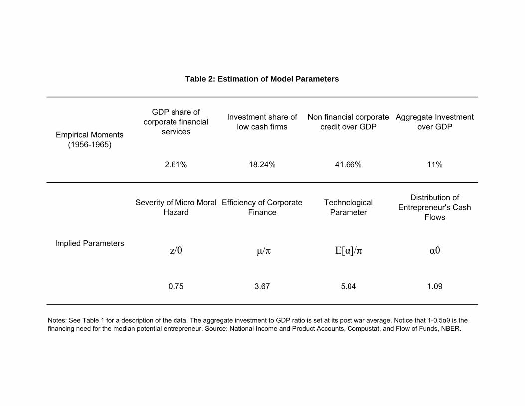
The data used in the estimation, and the implied parameters, are presented in Table 2.14

14The calibration is data intensive: it relies on long time series of aggregate and firm level measures, thatare only available for the US. See Greenwood, Sanchez, and Wang (2007) for a study of a large cross-sectionof countries.

19

4.1 Choice of standard parameters

I start by choosing standard values for the discount rate and for the depreciation rate:

Variable Empirical Value Model ParameterLength of 1 Period 20 yearsAnnual real rate 4% ρ = 1.0420 − 1Annual growth rate 2% γ = 1.0220 − 1Annual depreciation rate 6% δ = 1− 0.9420

Next, I use the fact that the book value of a realized project is 1 while its market value is

θ/ (ρ+ δ). I obtain θ by assuming a ratio of market value to book value of 2.15 To check

the robustness of the results, I have also calibrated the model with a period of 30 years and

market to book ratios from 1.5 to 2.5.

4.2 Empirical moments

It seems a priori difficult to calibrate the remaining parameters of the model, since they

are not observable. Notice, however, that the equilibrium equations (21) and (22) depend

only on the ratios μ/π and α/π. To reduce the degrees of freedom, I assume that fθ (.) is

uniform over£0, αθ

¤. The unknowns are therefore: z/θ, μ/π, α/π and αθ. I estimate the

four parameters using data on four observed quantities during the first decade, 1956-1965.

Investment over GDP

In the model economy, aggregate investment expenditures are equal to¡1− F θ (αl)

¢πn,

and the stock of capital along the balanced growth path is:

k =³1− F θ (αl)

´ πnθ

δ + γ.

The gross domestic product is αn + k. Therefore the investment share of GDP depends

only on αl and on the ratio α/π:

1− F θ (αl)

α/π + (1− F θ (αl)) θ/ (δ + γ).

I calibrate this ratio to 11% using private non-residential fixed investment divided by private

value added from the National Income and Product Accounts.15 In the model, θ is the market to book ratio of new firms. For all firms, Fama and French (2001) report

an asset weighted average of 1.4 over the period 1963-1998. On the other hand, for young firms, θ is largerthan 2 on average. Moreover, in the model, market to book is constant because agents are risk neutral andinterest rates are constant, so the model cannot capture time variations in market to book over time.

20

Capital expenditure share of low cash firms

The parameter α captures the ratio of income to capital expenditures, for the firms that

actually invest. I use a simple statistic to compare the model and the data: the share of

total investment accounted for by firms whose income is less than one third of their capital

expenditures.16 The investment share of low cash firms is based on Equation (1) in Section

1. In the model, it is:

s =³F θ (0.33)− F θ (αl)

´/³1− F θ (αl)

´.

Figure 5 displays the shares of investment accounted for by firms with α below 0.15, 0.25

and 0.33.

Corporate borrowing

In the model, firms with α < αl cannot invest, and firms with α > 1 can finance their

investment entirely with their current income (see Figure 8). Total corporate borrowing in

each period is therefore equal to:

πn

Z 1

αl

(1− α) dF θ (α) .

I compute the ratio of outstanding credit market instruments over GDP from the Flow

of Funds. This ratio is shown in Table 2. The relevant variable for the calibration is the

amount of new borrowing in each period. I assume that the average maturity of credit

market instruments is 10 years, and I calibrate the model to a borrowing ratio equal to

1/10 of the outstanding value from Table 1. For robustness, I have redone the calibration

assuming average maturities from 8 to 15 years for corporate bonds, and assuming that

fθ is downward sloping triangular instead of uniform. The quantitative properties of the

model are similar.

4.3 Implied parameters

Based on the evidence in Figure 4, I match 1 − n as 0.7 times the value added share of

the financial sector. This is why the target size for the financial sector is 2.26% in Table 2,

which is 0.6 times 3.8% from Table 1. In other words, the estimation assume that 1.51% of16This statistic is useful because it does not involve taking a ratio of income over capital expenditures. It

is robust to the discrepancy between the assumptions made in the model and the fact that firm sizes are infact very heterogenous. It also builds in the fact that large firms are more relevant than small firms

21

income is the share of financial services not captured by the model (transaction services to

households, etc.).

Table 2 shows the parameters implied by matching empirical moments. An important

parameter is the degree of moral hazard z. The estimation implies that moral hazard is

potentially severe. This is needed for the model to explain the amount of resources devoted

to corporate financial services.

Few empirical papers provide structural estimates of the severity of moral hazard or the

costs of external finance, but two notable exceptions are Biais, Bisière, and Décamps (2000)

and Hennessy andWhited (2007). Using firm level data and theoretical models, they provide

structural estimates of the severity of moral hazard, and of the costs of external finance.

This paper estimates the macroeconomic equivalent of these costs. In general equilibrium,

however, the price of external finance is endogenous, because it is always possible, though

not always optimal, to increase the number of agents working in the financial sector.

Biais, Bisière, and Décamps (2000) estimate large agency costs using a sample of French

firms in the 1990s. Hennessy and Whited (2007) find that the typical firm in their sample

behaves as if facing external costs of equity starting at 8.3% of gross proceeds, and rising

to about 14.5% when proceeds reach $100 millions. In the model, the average financing

fees are around 20% of proceeds, with significant heterogeneity since some firms have access

to direct finance, while others require significant monitoring. The implied parameters are

therefore consistent with the existing evidence.17

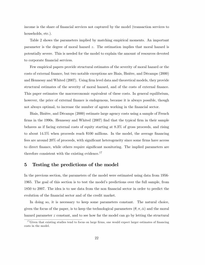
5 Testing the predictions of the model

In the previous section, the parameters of the model were estimated using data from 1956-

1965. The goal of this section is to test the model’s predictions over the full sample, from

1850 to 2007. The idea is to use data from the non financial sector in order to predict the

evolution of the financial sector and of the credit market.

In doing so, it is necessary to keep some parameters constant. The natural choice,

given the focus of the paper, is to keep the technological parameters (θ, π, α) and the moral

hazard parameter z constant, and to see how far the model can go by letting the structural

17Given that existing studies tend to focus on large firms, one would expect larger estimates of financingcosts in the model.

22

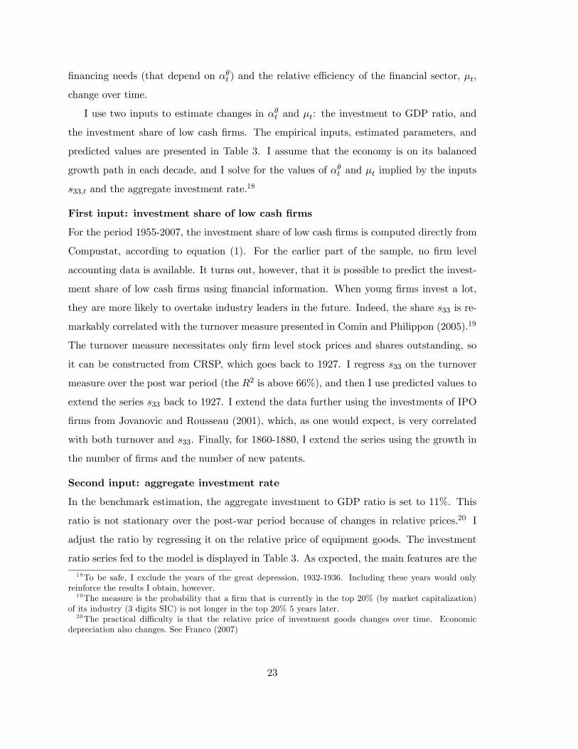
financing needs (that depend on αθt ) and the relative efficiency of the financial sector, μt,

change over time.

I use two inputs to estimate changes in αθt and μt: the investment to GDP ratio, and

the investment share of low cash firms. The empirical inputs, estimated parameters, and

predicted values are presented in Table 3. I assume that the economy is on its balanced

growth path in each decade, and I solve for the values of αθt and μt implied by the inputs

s33,t and the aggregate investment rate.18

First input: investment share of low cash firms

For the period 1955-2007, the investment share of low cash firms is computed directly from

Compustat, according to equation (1). For the earlier part of the sample, no firm level

accounting data is available. It turns out, however, that it is possible to predict the invest-

ment share of low cash firms using financial information. When young firms invest a lot,

they are more likely to overtake industry leaders in the future. Indeed, the share s33 is re-

markably correlated with the turnover measure presented in Comin and Philippon (2005).19

The turnover measure necessitates only firm level stock prices and shares outstanding, so

it can be constructed from CRSP, which goes back to 1927. I regress s33 on the turnover

measure over the post war period (the R2 is above 66%), and then I use predicted values to

extend the series s33 back to 1927. I extend the data further using the investments of IPO

firms from Jovanovic and Rousseau (2001), which, as one would expect, is very correlated

with both turnover and s33. Finally, for 1860-1880, I extend the series using the growth in

the number of firms and the number of new patents.

Second input: aggregate investment rate

In the benchmark estimation, the aggregate investment to GDP ratio is set to 11%. This

ratio is not stationary over the post-war period because of changes in relative prices.20 I

adjust the ratio by regressing it on the relative price of equipment goods. The investment

ratio series fed to the model is displayed in Table 3. As expected, the main features are the

18To be safe, I exclude the years of the great depression, 1932-1936. Including these years would onlyreinforce the results I obtain, however.19The measure is the probability that a firm that is currently in the top 20% (by market capitalization)

of its industry (3 digits SIC) is not longer in the top 20% 5 years later.20The practical difficulty is that the relative price of investment goods changes over time. Economic

depreciation also changes. See Franco (2007)

23

investment busts of the 1930s and 1980s, and the booms of the late 1960s and 1990s. These

medium-term fluctuations are consistent with the work of Comin and Gertler (2006).

Implied parameters

The implied parameters are presented in Table 3 and in Figures 9a and 9b. Figure 9a and

9b sheds light on the evolution of the US economy over the past 80 years. The 1920s are a

time a intense entry and investment by firms with large financial needs. These needs appear

constant until World War II, but the 1930s represent a financial disaster. The efficiency

of the financial sector collapses, and, as a result, a large number of firms become credit

constrained (the last column of Table 3 suggest that the fraction of credit constrained firms

doubles).

A structural shift happens during World War II. After the War, large established firms

with high cash flows appear to have the best investment projects. As a result, the demand

for financial intermediation collapses. Efficiency in finance recovers but remains below its

level of the 1920s for 3 decades. Credit constraints reach an all time low in the mid-1960s.

Over time, and especially since the 1970s, investment opportunities shift away from

large profitable firms and towards young firms with low current cash flows. There is a large

pent-up demand for intermediation that is not met because finance is not efficient enough.

In the 1990s, financial efficiency improves and leads to an investment boom. The structural

demand is remarkably stable however, suggesting that the bottleneck was the inefficiency

of the financial sector. In a sense, the 1990s look like the 1930s in reverse.

Interpretation and historical evidence

This interpretation of the structural demand parameters is supported by historical evi-

dence on General Purpose Technologies (David (1990)). The GPT of the early 20th century

was electrification. The GPT of the late 20th century was information technology. Jovanovic

and Rousseau (2005) argue that electrification corresponds to the period 1900-1930, with

much entry in the 1920s and the peak of adoption in 1929. IT starts in 1970, with much

adoption in the 1990s (figures 1, 2 and 3 in Jovanovic and Rousseau (2005)).

The historical consensus is that “startups, exits, patents, trademarks, and investment

by new firms relative to incumbents are higher during the GPT eras.” Moreover, “the ideas

and products associated with the GPT will often be brought by new firms.” In the model,

24

this corresponds to a shift in the distribution of opportunities towards low cash firms.

The 1950s and 1960s, by contrast, are periods where most innovations are performed

by large, profitable incumbents. In the model, this corresponds to shift in the distribution

of opportunities towards high cash firms. Once again, this is consistent with the historical

evidence.

On the supply side, there are two instances where finance seems to regress. The first, and

by far the largest, takes place during the 1930s. This is consistent with the banking collapse

and the tight regulations of the Great Depression. The second takes place in the 1980s,

and is consistent with the Savings and Loans crisis and the resulting disintermediation of

credit. The financial revival of the 1990s is consistent with anecdotal evidence, but I am

not aware of systematic evidence.

Actual and predicted size of the financial sector

Figure 10 shows the actual and predicted income shares of corporate finance services. The

actual value is the total share of the finance industry (from Table 1) minus 1.51% to remove

non-corporate financial services.21 The estimation of z/θ and α/π are such that the actual

and predicted size are the same in 1956-1965.

The model accounts for a surprisingly large fraction of the evolution of the financial

sector. It is important to emphasize that the quantitative predictions do not use any data

from the financial sector. The inputs are purely based on capital expenditures in the non-

financial sector.

One can think of Figure 10 as testing the predictions of the model for a broad measure

of credit spreads. For simple loans, the income of the intermediary is literally equal to the

volume of loans times the spread. In complex cases, Venture Capitalists for instance, there

is no simple spread, but the income share is still well defined. Predicting the income share

of the finance industry is therefore a very useful way to test the model.

Up to the 1990s, the model seems able to predict most of the changes in the size of the

financial sector. The model falls short in the more recent decade. Since the model forces21From Figure 4, I have set the share of corporate finance to 0.6 for the benchmark period. The adjustment

of 1.51% simply corresponds to 0.4 times the size of finance in 1956-1965. Note that I have subtracted afixed value of 1.51% instead of multiplying each period by 0.6, so that the actual changes in Figure 11 arethe same as the actual changes for the whole sector. This is both easier to interpret and more challengingto explain.

25

all the demand for financial services to come from domestic firms, the discrepancy could

reflect the globalization of the finance industry. There could also be an increase in financial

services provided to U.S. households. Alternatively, it could be that the financial sector is

too large and should be reduced.

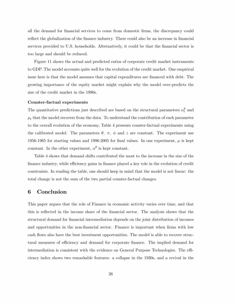
Figure 11 shows the actual and predicted ratios of corporate credit market instruments

to GDP. The model accounts quite well for the evolution of the credit market. One empirical

issue here is that the model assumes that capital expenditures are financed with debt. The

growing importance of the equity market might explain why the model over-predicts the

size of the credit market in the 1990s.

Counter-factual experiments

The quantitative predictions just described are based on the structural parameters αθt and

μt that the model recovers from the data. To understand the contribution of each parameter

to the overall evolution of the economy, Table 4 presents counter-factual experiments using

the calibrated model. The parameters θ, π, α and z are constant. The experiment use

1956-1965 for starting values and 1996-2005 for final values. In one experiment, μ is kept

constant. In the other experiment, αθ is kept constant.

Table 4 shows that demand shifts contributed the most to the increase in the size of the

finance industry, while efficiency gains in finance played a key role in the evolution of credit

constraints. In reading the table, one should keep in mind that the model is not linear: the

total change is not the sum of the two partial counter-factual changes.

6 Conclusion

This paper argues that the role of Finance in economic activity varies over time, and that

this is reflected in the income share of the financial sector. The analysis shows that the

structural demand for financial intermediation depends on the joint distribution of incomes

and opportunities in the non-financial sector. Finance is important when firms with low

cash flows also have the best investment opportunities. The model is able to recover struc-

tural measures of efficiency and demand for corporate finance. The implied demand for

intermediation is consistent with the evidence on General Purpose Technologies. The effi-

ciency index shows two remarkable features: a collapse in the 1930s, and a revival in the

26

1990s.

The quantitative predictions of the model regarding the size of the corporate credit

market and the income share of the financial sector are also supported by the data, except

for the most recent period. The model cannot account for the growth of the financial sector

between 2001 and 2006 based on the fundamental needs of the corporate sector.

There are several areas for future research. First, the model does not take into account

the services offered to households. Second, this paper does not address the issue of the

overall efficiency of the allocation of human capital between the financial and non-financial

sectors.22 Finally, future research should extend the quantitative analysis outside the US,

and take into account international trade.22Philippon and Reshef (2007) and Goldin and Katz (2008) document that finance attracts a growing

share of the economy’s top students. This prompts the question of the efficiency of this allocation.

27

References

Baumol, W. J. (1967): “Macroeconomics of Unbalanced Growth: The Anatomy of the

Urban Crisis,” American Economic Review, 57, 415—426.

Bekaert, G., C. R. Harvey, and R. Lumsdaine (2002): “Dating the Integration of

World Capital Markets,” Journal of Financial Economics, 65, 203—249.

Bencivenga, V. R., and B. D. Smith (1991): “Financial Intermediation and Endogenous

Growth,” Review of Economic Studies, 58, 195—209.

Biais, B., C. Bisière, and J.-P. Décamps (2000): “A Structural Econometric Investi-

gation of the Agency Theory of Financial Structure,” mimeo IDEI Toulouse University.

Carter, S., S. Gartner, M. Haines, A. Olmstead, R. Sutch, and G. Wright (eds.)

(2006): Historical Statistics of the United States Millennial Edition OnlineCambridge

University Press.

Comin, D., and M. Gertler (2006): “Medium-Term Business Cycles,” American Eco-

nomic Review, 96, 523—551.

Comin, D., and T. Philippon (2005): “The Rise in Firm-Level Volatility: Causes and

Consequences,” in Macroeconomics Annual, ed. by M. Gertler, and K. Rogoff. NBER.

David, P. A. (1990): “The Dynamo and the Computer: An Historical Perspective on the

Modern Productivity Paradox,” American Economic Review, 80(2), 355—361.

Davis, S., J. Haltiwanger, R. Jarmin, and J. Miranda (2006): “Volatility and Dis-

persion in Business Growth Rates: Publicly Traded versus Privately Held Firms,” in

Macroeconomics Annual, ed. by D. Acemoglu, K. Rogoff, and M. Woodford. NBER.

Diamond, D. W. (1984): “Financial Intermediation and Delegated Monitoring,” Review

of Economic Studies, 51, 393—414.

Do, Q.-T., and A. A. Levchenko (2007): “Comparative Advantage, Demand for Exter-

nal Finance, and Financial Development,” Journal of Financial Economics, 86, 796—834.

28

Fama, E. F., and K. R. French (2001): “Disappearing Dividends: Changing Firm

Characteristics or Lower Propensity to Pay?,” Journal of Financial Economics, 60, 3—43.

Fink, J., K. Fink, G. Grullon, and J. Weston (2005): “Firm Age and Fluctuations

in Idiosyncratic Risk,” Working Paper.

Franco, F. (2007): “Economic Change and the Aggregate Production Function,” mimeo

Universidade Nova de Lisboa.

Freixas, X., and J.-C. Rochet (1997): Microeconomics of Banking. MIT Press, Cam-

bridge.

Goldin, C., and L. F. Katz (2008): “Transitions: Career and Family Lifecycles of the

Educational Elite,” AEA Papers and Proceedings.

Gorton, G., and A. Winton (2003): “Financial Intermediation,” in Handbook Ot the

Economics of Finance, ed. by G. M. Constantinides, M. Harris, and R. Stulz, pp. 431—552,

North Holland. Elsevier.

Greenwood, J., and B. Jovanovic (1990): “Financial Development, Growth, and the

Distribution of Income,” Journal of Political Economy, 98, 1076—1107.

Greenwood, J., J. M. Sanchez, and C. Wang (2007): “Financing Development; The

Role of Information Costs,” Working Paper, University of Pennsylvania.

Hennessy, C. A., and T. M. Whited (2007): “How Costly Is External Financing?

Evidence from a Structural Estimation,” Journal of Finance, 62, 1705—1745.

Holmström, B., and J. Tirole (1997): “Financial Intermediation, Loanable Funds and

the Real Sector,” Quarterly Journal of Economics, 112, 663—691.

Jovanovic, B., and P. L. Rousseau (2001): “Why Wait? A Century of Life Before

IPO,” AER paper and proceedings, pp. 336—341.

Jovanovic, B., and P. L. Rousseau (2005): “General Purpose Technologies,” in Hand-

book of Economic Growth, ed. by P. Aghion, and S. Durlauf. Elsevier, Chapter 18.

29

King, R. G., and R. Levine (1993): “Finance and Growth: Schumpeter Might Be Right,”

Quarterly Journal of Economics, 108(3), 717—737.

Kuznets, S. (1941): “National Income and Its Composition, 1919-1938,” Discussion paper,

National Bureau of Economic Research.

Levine, R. (2005): “Finance and Growth: Theory and Evidence,” in Handbook of Eco-

nomic Growth, ed. by P. Aghion, and S. N. Durlauf, vol. 1A, pp. 865—934. Elsevier,

Amsterdam.

Martin, R. F. (1939): National Income in the United States, 1799-1938. National Indus-

trial Conference Board,.

Merton, R. C. (1995): “A Functional Perspective of Financial Intermediation,” Financial

Management, 24, 23—41.

Obstfeld, M., and A. M. Taylor (2002): “Globalization and Capital Markets,” NBER

Working Paper 8846.

Philippon, T. (2007): “Financiers versus Engineers: Should the Financial Sector Be Taxed

or Subsidized?,” Working Paper, NYU.

Philippon, T., and A. Reshef (2007): “Skill Biased Financial Development: Education,

Wages and Occupations in the U.S. Financial Sector,” NBER Working Paper 13437.

Philippon, T., and Y. Sannikov (2007): “Financial Development, IPOs, and Business

Risk,” mimeo, NYU.

30

A Appendix

Comparative staticsLet ∆ [.] denote the total difference of a function or a variable of interest. To prove thevarious propositions, I differentiate equation (21):

∆hμπ

i=³∆h απv

i−∆

hF θi(αl)

´m(αl) +

³ α

πv+ 1− F θ(αl)

´∆ [ml]−

Z αh

αl

∆hmdF θ

i,

and equation (22):µZ αh

αl

mdF θ +μ

π

¶∆ [n]

n=1− n

n∆hμπ

i−Z αh

αl

∆hmdF θ

i+m(αl)f

θ(αl)∆ [αl] .

These formula hold because the boundary terms with αl cancel out and becausem (αh) = 0.The monitoring function from equation (18) can be written as:

m (α) = z − θ + (ρ+ δ) (1− α) .

The total difference of this equation is:

∆ [m] = ∆ [z]−∆ [θ]− (ρ+ δ)∆ [α] +∆ [ρ+ δ] (1− α) .

Proof of proposition 1Consider first the limit when μ→ 0. First, rewrite (20) as

μ

πm(αl)=

α

πv+ 1− F θ (αl) +

Z αh

αl

µ1− m (α)

m(αl)

¶dF θ (α) .

As μ goes to zero, m(αl) also goes to zero and αl → αh. We need to evaluate the limit ofthe integral. For all α ∈ [αl, αh], we know that 0 < m (α) < m(αl) and therefore:°°°°Z αh

αl

µ1− m (α)

m(αl)

¶dF θ (α)

°°°° ≤ F θ (αh)− F θ(αl).

We can see that the integral goes to zero as μ goes to zero and:

limμ→0

μ

πm(αl)=

α

πv+ 1− F θ (αh) .

Using equation (22), we see that (1− n) /n = π/μR αhαl

mdF θ. Since the monitoring functionm is decreasing in α, it follows that°°°°Z αh

αl

m (α) dF θ (α)

°°°° ≤ m(αl)³F θ (αh)− F θ(αl)

´.

Since we have shown that μ/m(αl) has a finite limit, it follows that 1 − n → 0. In theother limit when μ → ∞, the result is clear from equation (22) since the integral of theright-hand-side is bounded by

R αh0

m (α) dF θ (α).Consider the impact of a change in μ. From equation (21), we see that

∆hμπ

i= − (ρ+ δ)

³ α

πv+ 1− F θ(αl)

´∆ [αl]

31

So it is clear that αh decreases with μ. The effect on the size of the finance industry,however, is ambiguous. From the monitoring market clearing (22), we see thatµZ αh

αl

mdF θ +μ

π

¶∆ [n]

n=1− n

n∆hμπ

i+m(αl)f

θ(αl)∆ [αl]

The sign of the RHS clearly depends on the value of n. QED.

For a change in z, we get

(ρ+ δ)³ α

πv+ 1− F θ(αl)

´∆ [αl] =

³ α

πv+ 1− F θ (αh)

´∆ [z]

So an increase in z increases αh. The effect on the size of the financial sector is ambiguous:

∆ [n]

n

µZ αh

αl

m (α) dF θ (α) +μ

π

¶= m(αl)f

θ(αl)∆ [αl]−³F θ (αh)− F θ (αl)

´∆ [z]

On the one hand, it takes more resources to monitor a given set of firms. On the otherhand, the pool of firms that are monitored shrinks.

32

PeriodGDP share of

corporate financial services

Investment share of low cash firms

Non financial corporate credit over

GDP

1860 1.13% 10.01% 14.41%

1870 1.01% 11.97% 17.94%

1880 1.02% 13.08% 25.54%

1890 1.58% 14.52% 32.22%

1900 2.27% 17.45% 36.24%

1910 2.22% 14.59% 45.53%

1920 2.51% 16.53% 44.49%

1930 3.39% 24.70% 57.31%

1940 2.42% 16.23% 50.31%

1950 2.03% 14.30% 41.83%

1960 2.61% 18.24% 41.66%

1970 2.87% 20.14% 49.87%

1980 3.31% 26.00% 68.48%

1990 4.24% 34.41% 78.65%

2000 5.21% 39.51% 86.75%

2007 5.57% 36.28% 87.52%

Notes: GDP share of corporate finance servies is 0.7 times the GDP share of all financial services. Investment share of low cash firms is the fraction of all capital expenditures in Compustat accounted for by firms whose income is less than one third of their capital expenditures. Before 1955, the investment share of low cash firms is estimated from turnover of industry leaders using CRSP. Before 1952, non financial corporate credit market is estimated using total corporate credit. Sources: National Income and Product Accounts, Annual Industry Accounts, CRSP, Compustat, Flow of Funds, and Historical Statistics of the United States.

Table 1: Data

GDP share of corporate financial

services

Investment share of low cash firms

Non financial corporate credit over GDP

Aggregate Investment over GDP

2.61% 18.24% 41.66% 11%

Severity of Micro Moral Hazard

Efficiency of Corporate Finance

Technological Parameter

Distribution of Entrepreneur's Cash

Flows

z/θ μ/π E[α]/π αθ

0.75 3.67 5.04 1.09

Table 2: Estimation of Model Parameters

Notes: See Table 1 for a description of the data. The aggregate investment to GDP ratio is set at its post war average. Notice that 1-0.5αθ is the financing need for the median potential entrepreneur. Source: National Income and Product Accounts, Compustat, and Flow of Funds, NBER.

Empirical Moments (1956-1965)

Implied Parameters

Periods Extra Prediction

10-year moving

averages around:

z/θ E[α]/πInvestment

Share of Low Cash

Firms

Aggregate Investment over GDP

μ/π αθCorporate Finance

GDP Share

Corporate Credit over

GDP

Corporate Finance

GDP Share

Corporate Credit over

GDP

Fraction of Credit

Constrained Firms

1860 0.75 5.04 10.0% 6.0% 2.39 0.86 1.45% 24.3% 1.13% 14.4% 20.0%

1870 0.75 5.04 12.0% 5.5% 2.51 0.84 1.40% 23.0% 1.01% 17.9% 17.8%

1880 0.82 4.87 493.2% 7.6% 2.54 0.82 2.04% 32.7% 1.02% 25.5% 25.1%

1890 0.75 5.04 14.5% 7.2% 2.52 0.76 2.15% 32.8% 1.58% 32.2% 26.4%

1900 0.75 5.04 17.5% 7.8% 2.60 0.72 2.57% 36.9% 2.27% 36.2% 29.4%

1910 0.75 5.04 14.6% 7.5% 2.55 0.77 2.20% 33.8% 2.22% 45.5% 26.4%

1920 0.75 5.04 16.5% 9.0% 3.25 1.00 2.17% 35.2% 2.51% 44.5% 16.6%

1930 0.75 5.04 24.7% 8.7% 3.04 0.70 3.21% 44.5% 3.39% 57.3% 26.6%

1940 0.75 5.04 16.2% 8.0% 2.63 0.76 2.44% 36.7% 2.42% 50.3% 27.7%

1950 0.75 5.04 14.3% 9.7% 3.27 1.13 2.03% 33.1% 2.03% 41.8% 15.5%

1960 0.75 5.04 18.2% 11.0% 3.67 1.09 2.61% 41.7% 2.61% 41.7% 14.7%

1970 0.75 5.04 20.1% 11.0% 3.75 1.04 2.82% 44.7% 2.87% 49.9% 14.7%

1980 0.75 5.04 26.0% 11.5% 4.43 1.01 3.37% 52.7% 3.31% 68.5% 9.0%

1990 0.75 5.04 34.4% 11.3% 4.37 0.79 4.35% 64.1% 4.24% 78.7% 11.5%

2000 0.75 5.04 39.5% 11.7% 4.87 0.77 4.92% 72.1% 5.21% 86.8% 5.9%

2007 0.75 5.04 36.3% 11.6% 4.74 0.81 4.54% 67.8% 5.57% 87.5% 7.3%

Notes: See Table 1 and 2 for a complete description of the data. The moral hazard and technology parameters are estimated in 1956-1965 (see Table 2), and are kept constant over time. The two implied parameters (efficiency of financial intermediation and structural financing needs of entrepreneurs) are estimated by matching two time-varying inputs: investment over GDP and the investment share of low cash firms. The model is then used to predict the size of the credit market and the share of income devoted to corporate finance services. The actual values are from Table 1. The corporate finance income share is the finance income share minus a fixed fraction of 1.51% corresponding to other financial services.

Realized Values

Table 3: Testing the Model's Predictions

Fixed parameters Inputs Implied Time-Varying Parameters Predicted Values

μ/π αθ Corporate Finance GDP Share

Fraction of Constrained Firms

Starting Values (from model) 2.63 0.76 2.25% 17.27%

Final Values (from model) 3.11 0.62 4.92% 5.94%

Predicted by demand shift only 3.16 0.59 3.47% 24.58%

Predicted by efficiency gains only 3.23 0.63 3.25% 4.77%

Table 4: Counter- Factual Experiments

Notes: Starting values correspond to 1956-1965. Final values correspond to 1996-2005. See Table 3. The model is non linear, so the effects are not additive.

Figure 1: GDP Share of U.S. Financial Industry

.08

.06

.04

.02

0

1860 1880 1900 1920 1940 1960 1980 2000

Source: Author’s estimation based on U.S. Annual Industry Accounts, Kuznet (1941), Martin (1939), U.S. Census, and Historical Statistics of the U.S. (2006).

Figure 2: GDP Shares of Finance Industries

0.045Credit Inter. Insur. Trusts & Funds Priv. Eq & Inv Bk

0.03

0.035

0.04

0.015

0.02

0.025

0

0.005

0.01

0.015

0

1977

1979

1981

1983

1985

1987

1989

1991

1993

1995

1997

1999

2001

2003

2005

Source: U.S. Annual Industry Accounts, Bureau of Economic Analysis

Figure 3: Allocations within the Financial Sector (2005)

0 5

0.6 Share of Finance GDP

Share of Finance Assets

0.4

0.5

0.2

0.3

0.1

0Credit Intermed. Insurance Trusts & Funds Priv. Eq & Inv Bk

Reading: The insurance industry accounts for 14.6% of the assets of the financial sector, and for 30.9% of its value added, in 2005. Source: Author’s calculations, U.S. National Income and Product Accounts, and Flow of Funds.

Figure 4: Estimates of the Share of Finance Activity related to Corporate FinanceCorporate Finance.

0 8

0.9

0.5

0.6

0.7

0.8

BASELINE

0.2

0.3

0.4

BASELINEBASE-ADMIN

0

0.1

1967

1970

1973

1976

1979

1982

1985

1988

1991

1994

1997

2000

2003

Notes: The baseline share is computed as one minus the compensation share of insurance specialists; traders of stocks, bonds,commodities and other assets; personal financial advisors; janitors, private security and miscellaneous employees. The second

b h h f d i i i k d l k S C P l i S d Phili d R h fmeasure subtracts the share of administrative workers and clerks. Source: Current Population Surveys, and Philippon and Reshef (2007).

Figure 5: Investment Shares of Low Cash Firms

0.5

0.6

s15 s25 s33

0.4

0.2

0.3

0

0.1

Notes: Sum of capital expenditures by firms whose income is less than 15% 25% or 33% of their capital

1955

1957

1959

1961

1963

1965

1967

1969

1971

1973

1975

1977

1979

1981

1983

1985

1987

1989

1991

1993

1995

1997

1999

2001

2003

2005

Notes: Sum of capital expenditures by firms whose income is less than 15%, 25% or 33% of their capital expenditures, divided by the sum of capital expenditures by all the firms in the sample. Source: Author’s calculations, Compustat sample of non financial firms.

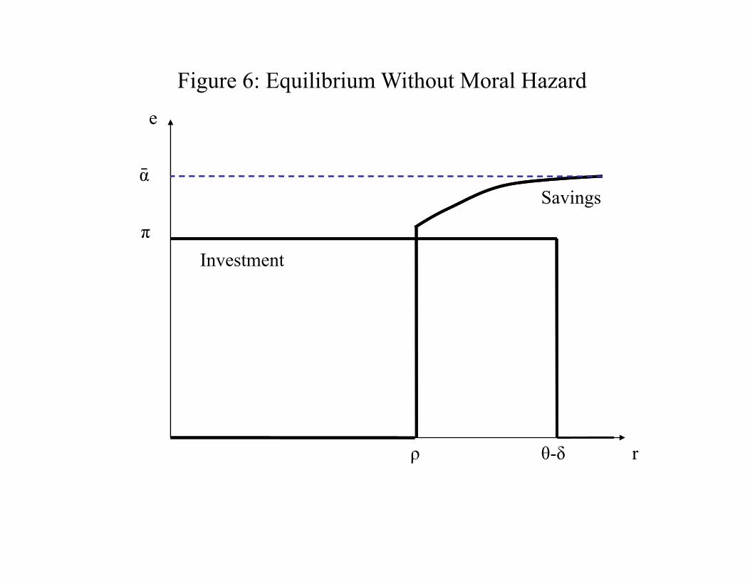
Figure 6: Equilibrium Without Moral Hazard

ᾱ

e

Savingsᾱ

πInvestment

rθ-δρ

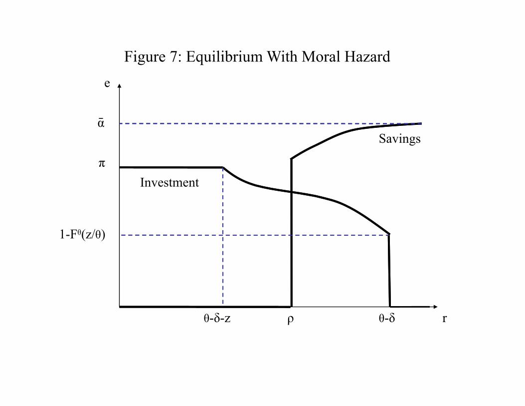
Figure 7: Equilibrium With Moral Hazard

ᾱ

e

Savingsᾱ

πInvestment

1-Fθ(z/θ)

rθ-δρθ-δ-z

Figure 8: Equilibrium With Monitoring

Density function fθ(α)

Constrained Invest

0 αl 1αh

αα

Monitored Direct Self-FinanceMonitoredFinance

DirectFinance

Self Finance

Figure 9a: Implied Structural Efficiency of U.S. Financial Industryp y y

2 10

Efficiency Index

1.70

1.90

2.10

1 10

1.30

1.50

0.70

0.90

1.10

0.501860 1870 1880 1890 1900 1910 1920 1930 1940 1950 1960 1970 1980 1990 2000 2007

Notes: The efficiency index is μ/π normalized to one in 1956-1965. The demand index is the external finance needed for the median project, 1-αθ/2.

Figure 9b: Implied Structural Demand for Corporate Financial Services

0 65

Demand Index

0.55

0.60

0.65

0.40

0.45

0.50

0.25

0.30

0.35

0.201860 1870 1880 1890 1900 1910 1920 1930 1940 1950 1960 1970 1980 1990 2000 2007

Notes: The efficiency index is μ/π normalized to one in 1956-1965. The demand index is the external finance needed for the median project, 1-αθ/2.

Figure 10: Predicted Size of Financial Sector

0.060

Income Share of Financial Sector(Corporate Finance Only)

0 040

0.050 Actual

Predicted

0.030

0.040

0.010

0.020

0.0001860 1870 1880 1890 1900 1910 1920 1930 1940 1950 1960 1970 1980 1990 2000 2007

Notes: Actual share is income share of finance and insurance minus the fraction that does not reflect corporate finance services (see Table 3). Predicted value constructed from estimated model using aggregate investment rate and s33 (investment share of low cash firms, and its predicted value before 1955) as inputs.

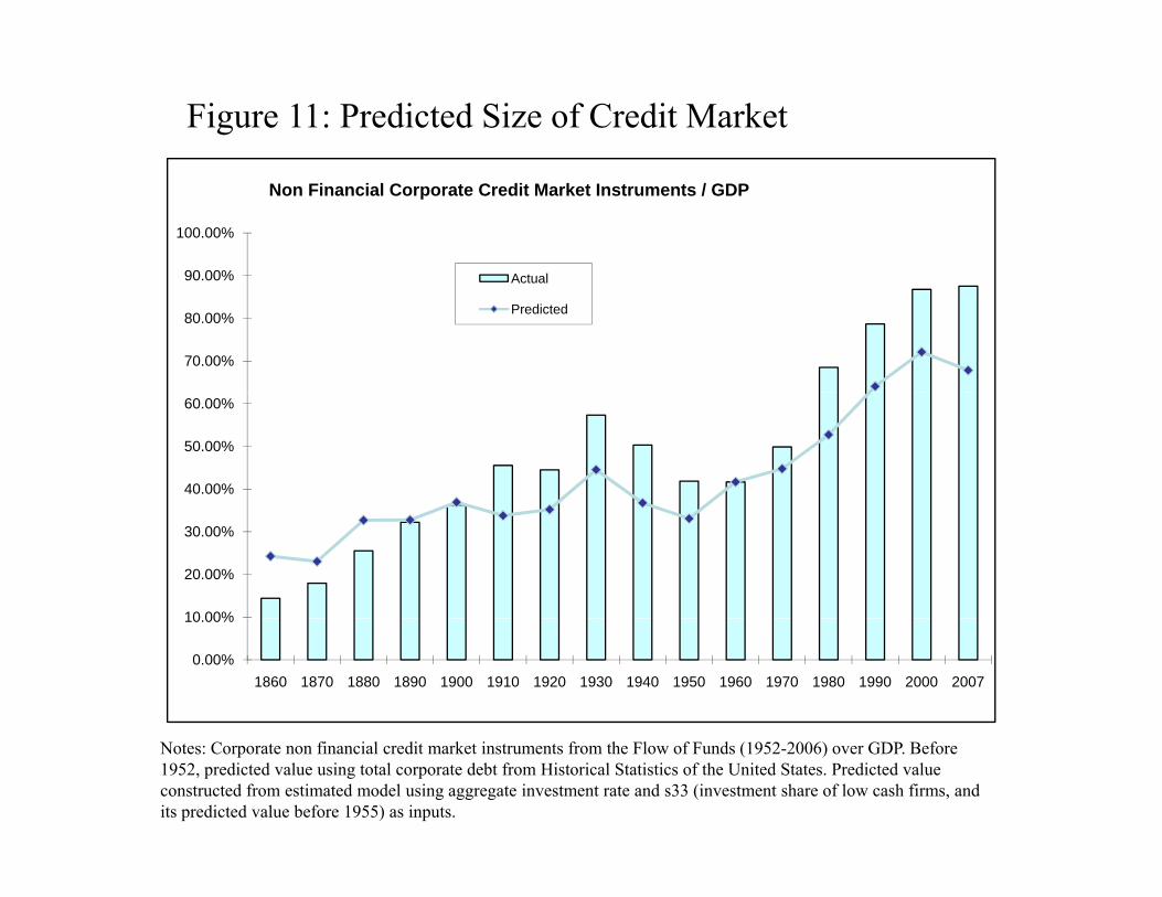
Figure 11: Predicted Size of Credit Market

90.00%

100.00%

Non Financial Corporate Credit Market Instruments / GDP

Actual

70.00%

80.00%

90.00% Actual

Predicted

40.00%

50.00%

60.00%

10 00%

20.00%

30.00%

0.00%

10.00%

1860 1870 1880 1890 1900 1910 1920 1930 1940 1950 1960 1970 1980 1990 2000 2007

Notes: Corporate non financial credit market instruments from the Flow of Funds (1952-2006) over GDP. Before 1952, predicted value using total corporate debt from Historical Statistics of the United States. Predicted value constructed from estimated model using aggregate investment rate and s33 (investment share of low cash firms, and its predicted value before 1955) as inputs.