THE EVOLUTION OF CENTRAL BANKING PRACTICES IN DEVELOPING

COUNTRIES: AN EFFECTIVENESS ANALYSIS ON THE POST-CRISIS

POLICY MIXES OF SELECTED COUNTRIES

A THESIS SUBMITTED TO

THE GRADUATE SCHOOL OF SOCIAL SCIENCES

OF

MIDDLE EAST TECHNICAL UNIVERSITY

BY

ZEYNEP BOZKURT

IN PARTIAL FULFILLMENT OF THE

REQUIREMENTS

FOR

THE DEGREE OF MASTER OF

SCIENCE IN

THE DEPARTMENT OF ECONOMICS

AUGUST 2015

Approval of the Graduate School of Social Sciences

Prof. Dr. Meliha Altunışık

Director

I certify that this thesis satisfies all the requirements as a thesis for the degree

of Master of Science.

Prof. Dr. Nadir Öcal

Head of Department

This is to certify that we have read this thesis and that in our opinion it is fully

adequate, in scope and quality, as a thesis for the degree of Master of Science.

Assist. Prof. Dr. Hasan Cömert

Supervisor

Examining Committee Members

Assoc. Prof. Dr. Şirin Saraçoğlu (METU,ECON)

Assist. Prof. Dr. Hasan Cömert (METU,ECON)

Assoc. Prof. Dr. Gökçer Özgür (Hacettepe, ECON)

iii

I hereby declare that all information in this document has been obtained

and presented in accordance with academic rules and ethical conduct. I

also declare that, as required by these rules and conduct, I have fully

cited and referenced all material and results that are not original to this

work.

Name, Last name: Zeynep Bozkurt

Signature :

iv

ABSTRACT

THE EVOLUTION OF CENTRAL BANKING PRACTICES IN DEVELOPING

COUNTRIES: AN EFFECTIVENESS ANALYSIS ON THE POST-CRISIS POLICY

MIXES OF SELECTED COUNTRIES

Bozkurt, Zeynep

MSc, Department of Economics

Supervisor: Assist. Prof. Dr. Hasan Cömert

August 2015, 169 pages

Implying an expansion in the central bank mandates and policy tools, the post-

crisis understanding of central banking brought a challenging task for

policymakers, particularly for those of developing countries. The main purpose of

this study is to assess the effectiveness of some selected post-crisis policy

mixes. To this end, two methodologies are used: event analysis and index

analysis. The former reveals that the overall design of the policy mix requires

more attention than the selection of certain tools – a fact that has been ignored

by the literature until this date. The study later digs deeper by introducing the

latter method. The Central Banking Effectiveness Index is developed in order to

obtain information where event analysis and empirical analysis fall short to

explain. Besides being one of the first attempts in the literature with such

purpose, the main contribution of this approach is the incorporation of the

interactions within the policy toolkit. The results from both analyses match. In

this respect, this study intends to fill an important gap in the literature and open

a way for prospective studies. The study also presents some important

implications upon the use of capital flow management tools and the patterns in

the selected developing countries – South Korea, Turkey and Brazil.

Keywords: Central Banking, Macroprudential Policy, Developing Countries

v

ÖZ

GELİŞMEKTE OLAN ÜLKELERDE MERKEZ BANKACILIĞININ EVRİMİ: SEÇİLEN

ÜLKELERİN KRİZ SONRASI POLİTİKA ÇERÇEVELERİ ÜZERİNE BİR ETKİLİLİK

ANALİZİ

Bozkurt, Zeynep

Yüksek Lisans, İktisat Bölümü

Tez Yöneticisi: Yard. Doç. Dr. Hasan Cömert

Ağustos 2015, 169 sayfa

Kriz sonrası merkez bankacılığı anlayışı merkez bankası hedefleri ve politika

araçlarında bir genişlemeye yol açmıştır. Böylelikle, başta gelişmekte olan

ülkelerde olmak üzere, merkez bankacılarının görevini daha zor hale getirmiştir.

Bu çalışmanın temel amacı kriz sonrasında oluşturulan bazı politika çerçevelerinin

etkililiğini değerlendirmektir. Bu amaç doğrultusunda iki yöntem kullanılmıştır.

Bunlar vaka analizi ve indeks analizidir. İlk yöntem, belirli araçların seçiminden

ziyade politika çerçevesinin genel tasarımına daha fazla önem atfetmek

gerektiğini ortaya koymaktadır. Günümüze kadar uzanan ilgili yazın bu noktayı

göz ardı etmiştir. Çalışma bir sonraki aşamada daha derinlemesine bir

değerlendirme yapmak amacıyla ikinci yöntemle devam etmektedir. Merkez

Bankacılığı Etkililik Endeksi, vaka analizi ve ampirik çalışmaların yetersiz kaldığı

koşullarda bilgi edinmek amacıyla oluşturulmuştur. Bu amaç için geliştirilmiş

öncü bir yöntem olmasının dışında, politika araçları arasındaki etkileşimleri

dikkate alması da bu yöntemin ilgili yazına önemli katkılarındandır. Yürütülen iki

analizin sonuçları birbiriyle örtüşmektedir. Bu bağlamda, bu çalışma yazındaki

önemli bir eksikliği giderme ve gelecek çalışmaların yolunu açma niyetindedir.

Çalışma ayrıca sermaye akımları yönetim araçlarının kullanımı ve seçili ülkeler

olan Güney Kore, Türkiye ve Brezilya’da görülen trendler hakkında da önemli

sonuçlar ortaya koymaktadır.

Anahtar Kelimeler: Merkez Bankacılığı, Makroihtiyati Politikalar, Gelişmekte

Olan Ülkeler

vi

To My Parents

vii

ACKNOWLEDGMENTS

I wish to express my deepest gratitude to my supervisor Asst. Prof. Dr. Hasan

Cömert for his guidance, advice, encouragements and insight throughout the

research.

I would like to thank Assoc. Prof. Dr. Şirin Saraçoğlu for her comments and

feedback.

The criticism and suggestions of Assoc. Prof. Dr. Gökçer Özgür are gratefully

acknowledged.

I also wish to express my sincere gratitude to my family and friends for their

support and trust throughout the process.

viii

TABLE OF CONTENTS

PLAGIARISM……………………………………………………………………………………………………………iii

ABSTRACT……………………………………………………………………………………………………………… iv

ÖZ…………………………………………………………………………………………………………………………… v

DEDICATION……………………………………………………………………………………………………………vi

ACKNOWLEDGMENTS…………………………………………………………………………………………… vii

TABLE OF CONTENTS……………………………………………………………………………………………viii

LIST OF TABLES………………………………………………………………………………………………………x

LIST OF FIGURES……………………………………………………………………………………………………xi

INTRODUCTION ........................................................................................ 1

2. THE EVOLUTION OF CENTRAL BANKING PRACTICES IN DEVELOPING

COUNTRIES: THE EMERGENCE OF THE NEED FOR MACROPRUDENTIAL POLICIES

2.1 OVERVIEW ................................................................................... 6

2.2 GREAT MODERATION: THE PATH TO THE GLOBAL FINANCIAL CRISIS .. 9

2.3 AFTER THE GLOBAL FINANCIAL CRISIS: THE RISE OF

MACROPRUDENTIAL POLICY ................................................................... 19

2.4 CLASSIFYING THE TOOLKIT: WHERE DO THEY STAND IN THE CYCLE? ..

.................................................................................................. 28

2.5 CHALLENGES FOR IMPLEMENTATION AND THE WAY AHEAD .............. 38

2.6 CONCLUSION............................................................................... 40

3. POST-CRISIS MONETARY POLICY FRAMEWORKS IN DEVELOPING COUNTRIES:

A CROSS-COUNTRY ANALYSIS ON THE NEW POLICY MIXES

3.1 OVERVIEW .................................................................................. 42

3.2 NEW POLICY MIXES ...................................................................... 45

3.3 LITERATURE REVIEW ON EFFECTIVENESS ANALYSIS ........................ 51

3.4 ASSESSING THE EFFECTIVENESS OF THE POST-CRISIS MONETARY

POLICY FRAMEWORKS IN THE SELECTED DEVELOPING COUNTRIES ............ 57

3.4.1 Volatility of Capital Flows and Exchange Rate............................. 58

3.4.2 Acceleration of Credit Growth and Asset Price Inflation ............... 71

ix

3.4.3 Overall Effects of the Policy Mixes on Financial Stability and Price

Stability ............................................................................................80

3.5 CONCLUSION ...............................................................................89

4. ASSESSING POST-CRISIS MONETARY POLICY FRAMEWORKS WITH A

CENTRAL BANKING EFFECTIVENESS INDEX: A COMPASS FOR THE UNCHARTED

TERRITORY

4.1 OVERVIEW ..................................................................................95

4.2 LITERATURE REVIEW ON INDICES ..................................................97

4.3 DATA AND METHODOLOGY .......................................................... 110

4.3.1 Standard CBRI ..................................................................... 111

4.3.2 Augmented CBRI and CBEI .................................................... 118

4.4 RESULTS ................................................................................... 126

4.5 ROBUSTNESS CHECKS ................................................................ 130

4.6 CONCLUSION ............................................................................. 137

5. CONCLUDING REMARKS ...................................................................... 141

REFERENCES .......................................................................................... 145

APPENDICES .......................................................................................... 152

APPENDIX A: THE TRENDS IN THE MAIN INDICATORS AMONG DEVELOPING

COUNTRIES ........................................................................................ 152

APPENDIX B: CORRELATION VALUES ...................................................... 155

APPENDIX C: RESULTS FOR THE ANALYSIS WITH FSI ............................... 157

APPENDIX D: TURKISH SUMMARY .......................................................... 158

APPENDIX E: TEZ FOTOKOPİSİ İZİN FORMU ............................................ 169

x

LIST OF TABLES

TABLES

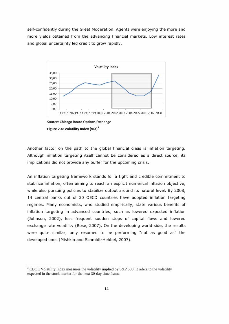
Table 2.1: The Expected Impacts of Some Selected Tools on the Steps of the

Cycle ...................................................................................................... 33

Table 2.2: Frequently Used Macro-prudential Tools in Some Developing Countries

.............................................................................................................. 35

Table 3.1: Coefficient of Variations for Gross Financial Inflows ....................... 60

Table 4.1: Monetary Policy Tools included in the Monetary Policy Index ......... 122

Table 4.2: CBRI and CBEI results (monthly) .............................................. 128

Table 4.3: CBEI results for Turkey computed with and without ROM ............. 131

Table 4.4: CBEI Values for Three Sub-Sample Periods ................................. 132

xi

LIST OF FIGURES

FIGURES

Figure 2.1: Real GDP Growth During Great Moderation ..................................11

Figure 2.2: Inflation Rates During Great Moderation ......................................12

Figure 2.3: The Relevance of New Consensus with the Global Financial Crisis ...13

Figure 2.4: Volatility Index (VIX) ................................................................14

Figure 2.5: Real Effective Exchange Rates in Some Developing Countries ........16

Figure 2.6: FX Reserves in Advanced and Developing Countries ......................17

Figure 2.7: Current Account Balance in Developing Countries .........................18

Figure 2.8: Credit and Residential Property Prices in Developing Countries .......18

Figure 2.9: Main Macroeconomic Indicators in Developing Countries (EM10) ....23

Figure 2.10: Inflation Rate in Developing Countries .......................................24

Figure 2.11: International Reserves in Developing Countries ..........................24

Figure 2.12: External Debt Indicators in Developing Countries .......................25

Figure 2.13: Credit and Asset Prices in Developing Countries .........................26

Figure 2.14: The Effects of Capital Inflows in Developing Countries .................31

Figure 3.1: Detailed Presentation of the New Policy Mixes of Selected Countries

..............................................................................................................45

Figure 3.2: Macroprudential Tools in Selected Developing Countries ................47

Figure 3.3: Net Capital Inflows over GDP in Selected Developing Countries ......59

Figure 3.4: Gross External Debt in Selected Countries ...................................62

Figure 3.5: Short-term Foreign Debt in Selected Developing Countries ............63

Figure 3.6: Effective Exchange Rates in Developing Countries ........................65

Figure 3.7: International Reserves as % of Gross External Debt .....................66

Figure 3.8: Volatilities of Selected Domestic Currencies .................................68

Figure 3.9: ROM Utilization Rate .................................................................69

Figure 3.10: Credit in Selected Developing Countries ....................................72

Figure 3.11: Loan Composition in S.Korean and Turkish Banking Systems .......73

Figure 3.12: Credit Growth in Selected Developing Countries .........................75

Figure 3.13: Residential Property Prices in S.Korea .......................................77

Figure 3.14: Residential Property Prices Indicators of Selected Developing

Countries .................................................................................................79

xii

Figure 3.15: The Gross Capital Inflows and Current Account Balances over GDP

.............................................................................................................. 81

Figure 3.16: Indicators for Currency and Maturity Mismatch in Selected

Developing Countries ................................................................................ 83

Figure 3.17: Investment Income in Selected Countries .................................. 84

Figure 3.18: CPIs of Selected Developing Countries ...................................... 85

Figure 3.19: Inflation Targets and Realized Inflation in Selected Developing

Countries................................................................................................. 87

Figure 3.20: GDP Growth Rates in Selected Developing Countries ................... 88

Figure 3.21: Total Unemployment Rates in Selected Developing Countries ....... 89

Figure 4.1: The Impossible Trinity .............................................................. 98

Figure 4.2: The Bell-Curves and Skewness Values for the Standard PTI’s of

Turkey and Brazil ................................................................................... 117

Figure 4.3: Z-values for the Standard PTI’s of Turkey and Brazil .................. 117

Figure 4.4: The Bell-Curve and Z-values for the Augmented PTI of Turkey..... 120

Figure 4.5: The Bell-Curve and Z-values for the Augmented PTI of Brazil ...... 121

Figure 4.6: The reasoning of CBRI and CBEI .............................................. 123

Figure 4.7: Co-movement of the sub-indices for responsiveness and

effectiveness analysis.............................................................................. 127

Figure 4.8: The Reasoning of the Main Indices ........................................... 131

Figure 4.9: The Strength of the Relationship Between the Turkish and Brazilian

PTI’s with VIX ........................................................................................ 133

Figure 4.10: Global Uncertainty in the Sub-Sample Periods Under Investigation

............................................................................................................ 135

1

CHAPTER 1

INTRODUCTION

After the global financial crisis hit the world economy, central banking took a

giant step forward in its evolutionary history. The implications of the crisis and

the circumstances of post-crisis environment forced policymakers to change their

previous perspective towards central banking practices.

The pre-crisis dominant view over the understanding of central banking, which is

known in the literature as the ‘New Consensus’, supported the idea that

managing solely price stability through short-term interest rates was sufficient to

promote both macroeconomic and financial stability. This simple way of

conducting monetary policy worked out fairly well during the ‘Great Moderation’

years, which led the support for the ‘New Consensus’ to gain strength and its

opponents to be neglected. By the same token, the stronger the ‘New

Consensus’ got, the more favorable conditions for the ‘Great Moderation’ took

place. By encouraging the neglect of financial stability and reluctance to react

against asset bubbles, this feedback loop set the stage for the global financial

crisis.

When the global financial crisis proved that this simple way of conducting

monetary policy was not sufficient to promote overall stability, policymakers had

to rethink their understanding of central banking. First, it was understood that

financial stability could not be considered as a second-order issue. Second,

indicators such as asset prices could not be neglected. Promoting a stable

inflation does not guarantee a well-functioning financial system. Counting on the

efficient market hypothesis lead policymakers lose time before intervening in any

disruptive trend within the financial markets. In line with these important

2

changes, an emerging consensus on central banking practices was born. Among

its multiple implications, this study focuses on three crucial ones. Firstly,

financial stability was included in the central banking mandates. Secondly, this

new mandate required some additional economic and financial indicators in the

control panels of central bankers. The pre-crisis set of targeted indicators –

inflation and GDP – widened significantly. Thirdly, the expansion of the set of

monitored indicators brought the need for additional tools in the policy toolkits of

central banks. Macroprudential policies were introduced or bolstered by the

central bankers worldwide with the aim of affecting a wide set of indicators which

are deemed to represent the circumstances in macroeconomic and financial

systems. These three major highlights of the post-crisis understanding of central

banking brought a difficult joint optimization problem for central bankers in

pursuit of overall stability. While transforming from the ‘New Consensus’ to the

emerging one, the understanding of central banking practices led a challenging

task for the policymakers worldwide.

Another implication of the global financial crisis is the need for advanced

countries to conduct non-conventional monetary policies. The post-crisis

environment in the wake of the crisis led central bankers of advanced countries

to develop exit strategies that were based on quantitative easing policies. These

policies formed an excess global liquidity. Similar to the case during the Great

Moderation, the excess liquidity ended up as capital flows into developing

countries. However, unlike the pre-crisis period, the excess liquidity entered into

the developing countries through capital inflows with a fluctuating global

uncertainty. Having already witnessed the bitter consequences of reliance on

global factors during the global financial crisis, the post-crisis economic

environment and the associated vulnerabilities had to be carefully dealt with.

Therefore, central bankers of developing countries were faced with even a more

challenging joint optimization problem which also had to take external conditions

into account. Considering the little experience with these tools and almost no

knowledge upon the interactions among them, the post-crisis era formed an

‘uncharted territory’ for central bankers.

The focus of this study is the challenging task of central bankers of developing

countries. The following Chapters assess this new era of central banking in

3

developing countries starting from mapping the risks for developing countries in

two integrated cycles: domestic and global. The first step is to determine the

reasons why developing countries needed differentiated policy mixes. It further

elaborates on the transmission channels that macroprudential tools are supposed

to overcome these problems. The assessment puts forward that each tool has

primary and secondary effects over the steps of the integrated cycles that

represents how risks are transmitted throughout the economy.

Another implication of this mapping is that central bankers may either suffer or

benefit from these secondary effects. A well-designed policy mix can achieve

efficacy and effectiveness by benefiting from the interactions within the toolkit.

Taking this crucial implication as a point of departure, Chapter 3 assesses the

post-crisis monetary policy frameworks of three selected developing countries:

Brazil, South Korea (S.Korea) and Turkey. These economies are both in the G20

and the “Fragile Five”, sharing some distinguishing features. Moreover, central

banks of all these three countries adopted and announced their adoption of new

policy mixes after the global financial crisis. Chapter 3 first aims to identify the

policy mixes adopted by each country and then to conduct a cross-country

analysis over the effectiveness of these policy mixes. The method for

assessment is event analysis. Although event analysis is a very conventional way

to conduct such an assessment, it still contributes to the literature in certain

ways. First, the analysis attempts to assess the effectiveness of post-crisis policy

mixes in a cross-country perspective. Related studies in the literature lack a

cross-country based perspective and rather focus on the case of a single country

in general. Secondly, none of the studies in the literature intends to take policy

interactions into account. The analysis provides some important findings. First,

the choice over the implementation of capital flow management tools appear to

be essential in countries with such economic and financial characteristics.

Second, in line with the implication from Chapter 3, the analysis in Chapter 4

also concludes that the design of the policy mix is more important than the

choice of individual tools. Some tools are found to be in interaction with others

that may have weakened the effectiveness of the toolkit in Turkey and Brazil

whereas S.Korean authorities enjoy more effectiveness and efficacy due to the

use of complementary tools. The findings also reveal that S.Korean economy has

significantly diverged from the trend observed in Brazil and Turkey, mainly after

4

2012. In terms of financial soundness, this can be considered as a divergence in

the positive direction. However, S.Korean policymakers seem to have neglected

the primary indicators – inflation and GDP – while having committed to promote

financial soundness.

Although Chapter 3 utilizes event analysis approach, the concluding remarks

over the trade-off within the policy mixes have some intuitive components. In

order to conduct an analysis that would enable us to quantitatively compute the

effectiveness that takes policy interactions1 into account, Chapter 3 develops a

new method. Taking the reasoning of Taylor rule as a point of departure, two

new indices to the literature are developed: A Central Banking Responsiveness

Index and Central Banking Effectiveness Index. The former assesses the extent

which central banks manage to cover the risks arisen in the monitored

indicators. In this sense, it puts forward the intuitive analysis in the previous

chapter that was conducted upon the mapping of macroprudential tools over the

integrated cycles. The latter, on the other hand, investigates the effectiveness of

the policy mixes, in other words, the numerical measure of the effectiveness of

the adjustments in the policy tools in addressing the movements in the

monitored indicators. The uniqueness of this approach is that this is the only

instrument in the literature that is developed to measure the effectiveness of

central banking practices. Moreover, it also takes the targets set by central

banks into account, which enables a realistic cross-country assessment with

customized indices. Regarding that the post-crisis conditions form an ‘uncharted

territory’ for central banking practices, the indices developed in this Chapter

carry an intention to be a ‘compass’ for policymakers in this ‘uncharted territory’.

Since Chapter 3 reveals that S.Korea has been following a significantly

differentiated trend mainly after 2012, the analysis in the last Chapter focuses

on the other two countries: Turkey and Brazil. These countries form an

appropriate base for comparative analysis regarding the risks faced by these

economies in the exchange rate, credit and capital flows fronts. The main

difference appears to be their use of tools in the capital flow management front.

While Brazilian authorities use capital flow management tools that were

1 The interactions cover both those within the macroprudential tools and conventional monetary

policy.

5

previously known as capital controls, Turkish policymakers prefer more market-

friendly measures. The findings reveal that Brazilian policy choices resulted in

more effectiveness, mainly by reducing the reliance on global factors. Moreover,

Chapter 4 also complements the results in Chapter 3 that the undesired policy

interactions between Turkish ROM, ended up with ineffectiveness of the tool. In

addition, further elaboration on the comparative analysis provided some other

findings upon the timely-implementation, commitment to targets and the

emphasis put on financial soundness.

In brief, the study is structured as follows: the first chapter is based on the

intention to point out the relevance of the Great Moderation and the New

Consensus with the global financial crisis. Focusing mainly on the case of

developing countries, the aim is to make clear how the pre-crisis conditions led

the emergence of need for macroprudential policy. Then the Chapter intends to

identify the steps of the risk cycle in developing countries and place

macroprudential tools in accordance with the transmission channels which they

are designed to block within the given cycle. Chapter 3 continues with the cross-

comparison of the policy mixes adopted by three selected developing countries:

Brazil, Turkey and S.Korea. The event analysis covers the indicators that stand

out to be the most common ones monitored by central banks according to

central bank reports and the related literature. The indicators are expected to

represent the conditions in both price and financial stability fronts. While trying

to assess the effectiveness of macroprudential tools individually, the Chapter

also makes an attempt to reach some insights upon the interactions of certain

tools. Finally, the last Chapter attempts to dig deeper by developing a Central

Banking Responsiveness Index and a Central Banking Effectiveness Index to

assess the extent of the coverage of risks and the effectiveness of the post-crisis

policy mixes in selected two countries: Turkey and Brazil. The aim is to conduct

a comprehensive quantitative assessment on the new policy mixes, while taking

policy interactions also into account.

6

CHAPTER 2

THE EVOLUTION OF CENTRAL BANKING PRACTICES IN

DEVELOPING COUNTRIES: THE EMERGENCE OF THE NEED FOR

MACROPRUDENTIAL POLICIES

2.1 OVERVIEW

Central banking has recently entered into a new era worldwide. This substantial

change occurred mainly due to the evolution in the understanding of central

banking. Driven by a rapid and giant step in the understanding, this change also

had massive impacts on the composition of central bank mandates, the policy

toolkit and the institutional framework. The importance of international

cooperation is highlighted. More importantly, unlike before, central banks

adopted new policy mixes that are designed to address the risks that are specific

to their economies, especially in developing countries. The particular focus of

this Chapter is the policy toolkit in developing countries that has been enhanced

in line with the extension of central bank mandates.

The Chapter first focuses on the pre-crisis period known as the ‘Great

Moderation’, which set the stage for the new era in central banking. A few years

ago, when central bankers used to control price stability only through short-term

interest rates, the common view implied that this was the best way to implement

monetary policy. Pleasant trends in the main indicators of the time also helped

this view which is known as the ‘New Consensus’ to gain strength. On the other

hand, as the New Consensus became more widespread, fewer concerns were

raised about the execution of monetary policy. A feedback loop between these

two concepts eventually brought the most drastic punctuation in the equilibrium

– the global financial crisis. In this respect, one of the main attempts of this

7

study is to shed light on the Great Moderation which prepared the conditions for

the global financial crisis and led a drastic change in central banking. Having

already been studied extensively in the literature, the points mentioned above

still require emphasis since they form a basis for the rest of the study to

elaborate further on the case of developing countries.

With the global financial crisis taking place, the most commonly accepted views

on the execution of monetary policy were proven to be wrong, or insufficient at

least. Following the collapse of the New Consensus, a new one emerged. The

understanding of central banking practices of the post-crisis period differs from

that of the pre-crisis in several ways. Nevertheless, this Chapter focuses on two

main ones that came along with the collapse of the pre-crisis consensus. First,

the importance of financial stability was highlighted. It was understood that

financial stability could not be considered as a second-order issue while pursuing

an overall stability. Although central banks have always had a microeconomic

function in addition to their macroeconomic duty, financial stability took its place

near price stability in the list of central bank mandates for the first time in the

history of central banking. Second, the need to monitor and manage the

movements in the asset prices was underlined as a lesson from the global

financial crisis. Along with the inclusion of financial stability in the central bank

mandates, adding asset prices in the control panel of central bankers brought

the need for additional tools to deal with multiple goals. The use of

macroprudential policies have become much more widespread, being introduced

or bolstered by the central banks of almost every country as well as some

measures that are taken at the international level. Therefore, another attempt of

this Chapter is to elaborate on these massive changes with a particular focus on

the extended use of macroprudential policies.

While central banks worldwide are in the course of adapting to this new

understanding and its implications, the task of the central bankers in developing

countries is even more challenging. The global financial crisis drew attention

back to a well-known struggle for developing countries – minimizing the

dependence on external conditions. The magnitude and composition of capital

flows into developing countries have crucial impacts on the domestic

macroeconomic and financial systems. Moreover, the transmission of volatility

8

between the domestic and global conditions has been a major source of problem

for central bankers in pursuing their policies. These challenges were highlighted

both during and after the global financial crisis with frequent fluctuations in the

global uncertainty. Therefore, policymakers of developing countries have been

working on, or already introduced a set of macroprudential tools to deal with the

specified issues. To fully understand these integrated cycles and the tools that

are designed to mitigate the risks arising from them, the last attempt of this

Chapter is to develop a new classification method for macroprudential policies.

Unlike other classification models in the literature, the one presented in this

Chapter lists the tools according to the step in the cycle that they are designed

to address, instead of listing them only by their types. This way of classification

is more beneficial while studying the impacts of the tools on the monitored

indicators. It allows us to observe the multiple steps of the cycle that a tool is

capable to affect through indirect impacts as well as the step that a tool is

designed to address in a direct manner. This way, the Chapter can draw a

detailed picture on the way which macroprudential tools are expected to help

policymakers to deal both with macroeconomic and financial systems.

Having these three main attempts to explain in its focus, this Chapter is

structured as follows: The first section explains the main characteristics of the

Great Moderation. Its main components and neglects which gave birth to the

crisis are presented. Section three focuses on the post-crisis period, particularly

on the main changes occurred in the understanding of central banking and the

reasons that brought the rise of macroprudential policy. The fourth section

elaborates further on the case of developing countries, investigating the standing

of macroprudential tools in the policy toolkits. The integrated external and

domestic cycles for developing countries are presented. Macroprudential tools

are mapped within the cycle, according to their main purposes. Lastly, the

challenges for the implementation of macroprudential policies are underlined and

a conclusion is given to resume the highlights of the Chapter.

9

2.2 GREAT MODERATION: THE PATH TO THE GLOBAL FINANCIAL

CRISIS

In the mid-2000s, almost the whole world was experiencing a period called the

“Great Moderation” which implied low volatility, controlled inflation and growing

economies. This bright atmosphere led the view that managing inflation by

simply manipulating the overnight interest rates was sufficient to promote

overall macroeconomic stability. This dominant view is referred as the ‘New

Consensus’. The credit for the favorable conditions of Great Moderation was

given to successful monetary policy by the supporters of the New Consensus. In

Bernanke's (2004) words, “the improvements in the execution on monetary

policy can plausibly account for a significant part of the Great Moderation”.

Another similar view resumed that “the worldwide progress in monetary policy is

a great achievement that, especially when viewed from the perspective of 30

years ago, is a remarkable story” (Goodfriend 2007:65).

Although the ‘New Consensus’ was the dominant view, there were some debates

over its main assumptions. There were some cautious approaches upon the

effectiveness of the monetary policy and studies asserting that this picture might

be illusive. However, the favorable conditions of mid 2000s caused central

bankers to stick with their existing policies and therefore led some crucial

neglects.

To explain the main characteristics and the debates over them, first of all the

time span of Great Moderation should be determined. It is possible to consider

Great Moderation in two separate phases: the first phase of 1990s and the

second phase of 2000s. As the date of its end, this study takes the first quarter

of 2007, following the study of Aizenman et al. (2010)2.

The first phase of 1990s has two main implications. First, world economies

entered into a new era of more open capital accounts and deep financial

integration. These developments set the stage for availability for higher yields.

The second implication is the crises that took place in developing countries.

2 They set the last quarter of the Great Moderation based on the movements in the CBOE S&P 500

VIX, LIBOR-IO Spread, EMBI.

10

Crises such as the Mexican in 1994-95 and East Asian in 1997 led policymakers

to promote stronger economic and financial fundamentals. During the first

phase, advanced countries have already entered into an era of lowered volatility

and pleasant macroeconomic indicators.

In the second phase, with the promotion of stronger economic and financial

fundamentals in developing countries, low volatility and pleasant trends in

macroeconomic indicators became widespread worldwide. Moreover, the central

banking practices have almost harmonized in both developing and advanced

countries. This harmonization was due to some widely accepted views – “ New

Consensus” – over the understanding of central banking practices. It is possible

to summarize the main characteristics of the New Consensus under three main

headings, that the major neglects of the era can be discussed: the dichotomy

between price stability and financial stability; the ‘Lean vs. Clean’ debate; and

inflation targeting frameworks with floating exchange rate regimes. To better

understand how these characteristics gave rise to the global financial crisis, the

links between these main points and the components of Great Moderation should

be investigated.

The macroeconomic view during the Great Moderation regarded price stability

and financial stability as two separate matters. In fact, most of the central banks

were aware of the problems arisen from financial frictions and a large number of

them were already publishing Financial Stability Reports. However, the

Tinbergen rule –which implied the need for the use of separate tools for different

objectives - was highly accepted as a principle for central banking practices

among policymakers. The Tinbergen rule required monetary policy to address

price stability and prudent regulation and supervision -especially microeconomic

policy which aims to mitigate risks at an individual institution level- to address

financial stability. The general equilibrium modelling frameworks of most central

banks did not consider financial frictions as a major source of business cycle

fluctuations. An inflation-targeting central bank could assert that it coped with

credit market excesses automatically insofar since higher asset prices boost

aggregate demand and create inflationary pressures (Eichengreen et al., 2011).

Therefore, price stability was deemed to be sufficient in the promotion of

financial stability and macroeconomic stability.

11

Other economists and central bankers, who do not share the perspective of the

New Consensus, were concerned that financial markets, being more integrated,

competitive and innovative, were reducing the effectiveness of the monetary

policies of the central banks. The influence of central banks on long-term interest

rates seemed to be weakening (Cömert, 2012; Rudebush et al., 2006) The main

drawback of this rapid integration was the central banks’ weakness on controlling

financial markets.

The following figures demonstrate the main macroeconomic variables that were

closely monitored during Great Moderation. Figure 2.1 shows that during the

period from early 2002 to mid-2007 the real GDP growth in emerging and

developing economies rose by nearly 122%. Similarly, advanced countries

enjoyed an almost doubled GDP growth rate through the end of the given period.

Source: IMF World Economic Outlook Database

Figure 2.1: Real GDP Growth During Great Moderation

Furthermore, Figure 2.2 clearly demonstrates that during the same time span

inflation was remarkably controlled worldwide. The average inflation rate

worldwide remained below 5% during the years under investigation. Within the

same time span, the rate was around 6% in developing and 2-3% in advanced

countries.

12

Source: IMF World Economic Outlook Database

Figure 2.2: Inflation Rates During Great Moderation

Another component of the consensus of “Great Moderation” is the Greenspan

doctrine. During the Great Moderation years, there had been a heated debate

over whether and how central banks should respond to asset price bubbles.

Greenspan (2002) was a strong opponent of such response by central banks,

stating that monetary policy should clean up after an asset price bubble bursts,

rather than leaning against them. This view has been supported by several

arguments in the literature.

The first and the most common argument against leaning a bubble is that an

asset price bubble is hard to detect. The assumption that central banks have

such an informational advantage over private markets to identify a bubble in

progress is highly dubious (Hahm et al.,2012). Secondly, bubbles are defined as

deviations from fundamentals, which make them unlikely to respond to usual

tools of monetary policy. Asset prices bubbles may not respond to moderate

changes in interest rates whereas drastic changes may cause more harm than

good by depressing economic growth and increasing output volatility

(Eichengreen et al., 2011). Moreover, leaning against a specific type of asset

price bubble would also have unintended effects on other types of asset prices.

Lastly, as Giavazzi and Mishkin(2006) put it, addressing asset prices may lead

confusion of central bank objectives in public and cause a weakening of

confidence.

13

Although the Greenspan doctrine was widely adopted by central bankers in

pursuit of monetary policy decisions, there is a wide literature in favor of leaning

against asset price bubbles. Cecchetti et al.(2000), Borio and Lowe(2002) and

White (2004) are some of the studies which argue that central banks should

raise interest rates to slow down accelerating asset prices and thus save the

economy from getting damaged at least up to some extent.

Figure 2.3: The Relevance of New Consensus with the Global Financial Crisis

The chain of events given Figure 2.3 above summarizes how the impacts of the

two main components of the New Consensus turned out to be the background

for the global financial crisis. As an implication of the New Consensus, central

bankers remained reluctant to react against the extreme movements in credit

growth and asset prices. This led an expansion in the balance sheets of financial

institutions and encouraged lending and borrowing behavior further. While the

circumstances for a housing bubble were being set, the fact that central bankers

also neglected the need for sufficient financial regulation and supervision

speeded the process up. Apart from these two points of departure, there were

also some other factors contributing the uncontrolled subprime lending.

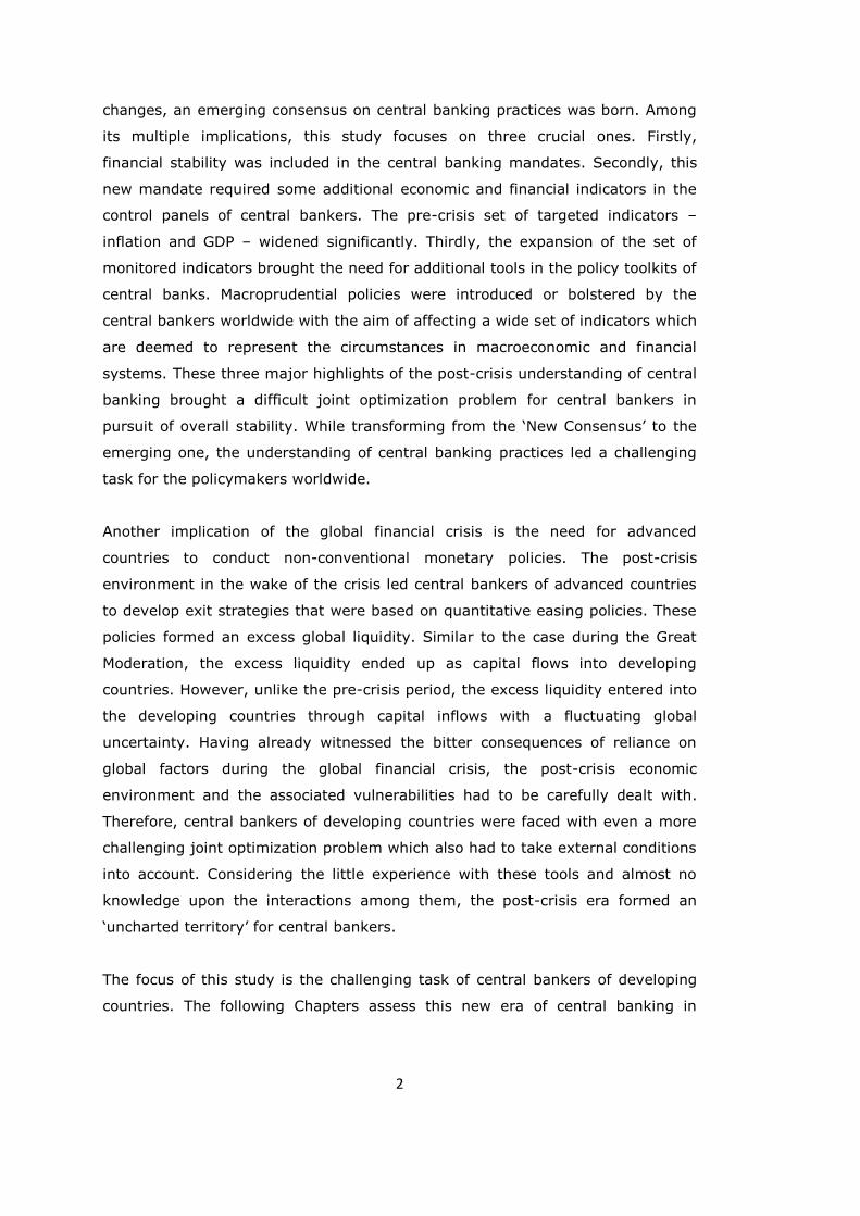
The favorable conditions of Great Moderation also led a gradual decline in the

global uncertainty. By the same token, the fall in the VIX encouraged agents in

the economy to take broader risks. Policymakers allowed credit growth to run

free, promoting the appetite for further risk for yield. The volatility in the world

markets had reached the lowest values just before the global financial crisis, in

2005 and 2006 (Figure 2.4). Furthermore, the central bank of the most

advanced financial market in the world, Fed, was providing low interest rates,

Subprime Lending

Further lending/borrowing

No need to react against bubbles

Lean vs Clean Debate

Lack of regulation No need for

financial regulation and supervision

The Dichotomy Between Price Stability and

Financial Stability

14

self-confidently during the Great Moderation. Agents were enjoying the more and

more yields obtained from the advancing financial markets. Low interest rates

and global uncertainty led credit to grow rapidly.

Source: Chicago Board Options Exchange

Figure 2.4: Volatility Index (VIX)3

Another factor on the path to the global financial crisis is inflation targeting.

Although inflation targeting itself cannot be considered as a direct source, its

implications did not provide any buffer for the upcoming crisis.

An inflation targeting framework stands for a tight and credible commitment to

stabilize inflation, often aiming to reach an explicit numerical inflation objective,

while also pursuing policies to stabilize output around its natural level. By 2008,

14 central banks out of 30 OECD countries have adopted inflation targeting

regimes. Many economists, who studied empirically, state various benefits of

inflation targeting in advanced countries, such as lowered expected inflation

(Johnson, 2002), less frequent sudden stops of capital flows and lowered

exchange rate volatility (Rose, 2007). On the developing world side, the results

were quite similar, only resumed to be performing “not as good as” the

developed ones (Mishkin and Schmidt-Hebbel, 2007).

3 CBOE Volatility Index measures the volatility implied by S&P 500. It refers to the volatility

expected in the stock market for the next 30-day time frame.

15

Inflation targeting regime contributed to the set-up of the global financial crisis

in the sense that it required only the monitoring of inflation and real GDP

growth. Central banks were deemed to be successful depending on whether they

hit their pre-announced targets. As stated before, central bankers were

responsible from the extreme movements of the asset prices only if they had

significant effects on the inflation rate. To this end, the limited control panel

required by an inflation targeting regime of the time led crucial neglects.

The conditions that facilitated the subprime lending were further promoted by

the developments in the financial instruments. US, having the most advanced

but also complex financial market continued improving with financial

innovations, particularly with the integration of derivatives to this leading

market. However, as indicated before, this complex market lacked sufficient

regulations. The tools available fell short in measuring the risk arising from those

financial instruments properly. Brokers who were providing credits had no

responsibility afterwards, which gave rise to the possibility of uninformed

homeowners misunderstanding some crucial terms and proceeding problems in

payments. Furthermore, mortgages were repacking over and over to other

banks. Eventually, these collateralized debt obligations have formed the grounds

of the global financial crisis.

As in advanced countries, central bankers of developing countries were also

celebrating since they were able to hit their inflation targets, promote high

growth rates and low volatility. By 2008, nearly 20 developing countries adopted

inflation targeting regimes. As clearly seen from the two main indicators to

monitor at that time (Figure 2.1&2.2 earlier), they assumed that they were doing

well. However, several studies reveal that their success may not have been

achieved only by effective control of short-term interest rates and promoting

price stability does not mean that they reached an overall macroeconomic

stability.

In a study upon the success of South African inflation targeting, Comert and

Epstein (2011) argue that the South African experience with inflation targeting

was not successful when considered in terms of achieving low employment and

higher economic growth. In other words, even though they were able to hit the

16

targets, the main macroeconomic variables were not doing well. Furthermore,

Heintz and Ndikumana (2011), questioning the performance of developing

countries on the inflation targets, state that during the period in which inflation

targets were met, the real exchange rate was persistently appreciating.

In the same vein, the success of another developing country, Turkey, in inflation

targeting is also being questioned. Benlialper and Comert (2013) argue that

tolerating Turkish lira when it appreciated and intervening when it depreciated,

which they call “implicit asymmetric exchange rate peg” under the inflation

targeting regime, is the main reason that inflation targets were hit at that time.

In other words, the Turkish central bank has benefited from the appreciation in

Turkish lira as an implicit tool, to hit their inflation targets.

The findings of these studies are also supported by the study of Aizenman et al.

(2008). In their study conducted on 17 emerging market countries, they find

strong evidence that inflation targeting emerging economies have been following

a mixed inflation targeting strategy whereby central banks respond to both

inflation and real exchange rates in setting policy interest rates.

Source: BIS

Figure 2.5: Real Effective Exchange Rates in Some Developing Countries

Figure 2.5 verifies the fact that developing countries, some significantly and

some moderately experienced an appreciation trend during Great Moderation.

Considering the evidence from the literature and the appreciation trend which

lasted until around the last quarter of 2008, it is likely that the well performance

17

of central banks with their inflation targets might have been provided by the

appreciation of domestic currency. The appreciation trend is likely to be

associated with international capital flows led by expanding balance sheets in

advanced countries. Moreover, Figure 2.6 below demonstrates that the foreign

exchange reserve accumulation followed a significant upward trend, which

strengthens the given argument. Figure 2.7 also supports the findings that the

current account surplus in developing countries was rising for the given time

frame. If developing countries used exchange rates as an implicit tool, it is very

likely again, that most of them have ignored the undesired consequences of

over-appreciation in developing countries (Benlialper, Comert, 2013).

Source: IMF

Figure 2.6: FX Reserves in Advanced and Developing Countries

In this respect, an implication of the Great Moderation for developing countries

was their standing in the middle ground of the challenging ‘impossible trinity’.

The large accumulation of reserves provided them to enjoy some degree of

monetary autonomy and open capital accounts. At the same time, the underlying

factors that enable this large reserve accumulation as well as the availability of

open capital accounts led the currency appreaciation and therefore a successful

record of inflation targeting.

18

Source: IMF

Figure 2.7: Current Account Balance in Developing Countries

The excess global liquidity driven by the expanding balance sheets in advanced

countries had significant impacts also on the domestic credit cycles of developing

countries as well. Within the same time framework, the credit provided to

private sector increased by 48% and residential property prices rose by 34%

(Figure 2.8).

Source: WorldBank, BIS

Figure 2.8: Credit and Residential Property Prices in Developing Countries

Since increasing short-term interest rates as a measure would lead further

fueling of the cycle, developing economies experienced a serious policy dilemma

and had to let procyclicality persist. Only some East Asian countries adopted

19

some measures in order to curb the mortgage lending and addressed the

housing sector explicitly.

As stated in the beginning of this section, developing countries strengthened

their main macroeconomic and financial fundamentals after their own financial

crises in 1990s. This amelioration made these countries more investable for

international investors. With more open capital accounts and more levered

system, developing countries attracted large capital inflows during the second

phase of the Great Moderation. This allowed their domestic currencies to

appreciate and facilitated the task of policymakers to hit the preannounced

inflation targets. Moreover, with the acceleration in credit growth and asset price

inflation to some degree, the real GDP growth was fueled. Nevertheless, these

favorable conditions made emerging economies dependent on the global

conditions. Becoming dependent on international capital inflows in order to

promote domestic macroeconomic stability brings the risk for developing

countries to be extremely sensitive to a sudden stop or reversal. Counting only

on the surge of capital inflows and the accumulation of international reserves

proved to be insufficient with the onset of the global financial crisis.

2.3 AFTER THE GLOBAL FINANCIAL CRISIS: THE RISE OF

MACROPRUDENTIAL POLICY

The global financial crisis has been a dramatic challenge to central banks,

shaking the foundations of the pre-crisis consensus (Goodhart, 2010).

Economists and central bankers have realized that financial stability should have

counted more than a second-order issue, a fact that they have been ignoring in

the course of Great Moderation. Central banks thought that financial instability

could endogenously be managed due to the efficient market hypothesis and its

effects on the real economy could be handled the by monetary policies

implemented mainly for the price stability (Carré, 2013). These were proven to

be wrong. The crisis clearly underlined the importance of financial stability and

the need to more pay attention to it. In this vein, central banks started to seek

appropriate ways to manage both price stability and financial stability.

20

Besides these massive changes in the understanding of central banking practices

after the global financial crisis, there have also been some views that haven't

changed. First, a majority of central bankers and economists share the idea that

price stability should still serve as the primary objective (IMF 2010, De Gregorio,

2010). Secondly, the policy framework with flexible inflation targeting is still

seen as valid since the goal of maintaining low inflation is inescapable and the

pre-announced target establishes a benchmark for accountability (Mminele,

2010). However, although the basic central banking paradigm of flexible inflation

targeting is still valid, the form of its flexibility requires substantial rethinking

(Mishkin, 2012).

Due to some reasons driven by this massive change, the policy toolkit of central

bankers required an expansion. First, since monetary policy failed to meet the

policy needs of central banks in dealing with the global shock after the crisis,

central bankers used unconventional monetary policy tools as an exit strategy.

Many advanced economies cut policy rates at historical low levels for prolonged

periods and expanded systemic liquidity. They also adopted the role in the

resolution of systemically important institutions. On the other hand, facing with

the bitter consequences of financial imbalances and procyclicality, they realized

the importance of monitoring financial stability and countercyclical policies. The

challenge faced by central banks was the fact that monetary policy was not

sufficient in pursuing both price stability and financial stability. Monetary policy

can be constrained by the exchange rate regime, the prevalence of foreign

currency lending or an inefficient policy transmission mechanism (Lim et al.,

2013). Furthermore, using simply short-term interest rates prevents central

banks from addressing specific sectors such as housing market. In addition,

solely regulating individual institutions by microprudential policies also did not

guarantee financial stability. To this end, central banks found the solution in an

alternative policy to prevent the build-up of systemic financial risks, which is the

macroprudential policy.

Therefore, in brief, the post-crisis central banking is associated with the following

highlights: financial stability complements price stability as a central bank

mandate whereas price stability continues to be the primary objective; inflation

targeting regimes remain in use as before, but with more flexibility; the control

21

panel of central banks no longer consists only of inflation and output but also

include some other crucial macroeconomic and financial indicators; pursuing

both mandates and monitoring a wider set of indicators bring the need for

additional policy tools in the toolkit of central bankers.

In the light of these recent developments, financial regulators of the developed

world, such as Bank for International Settlement (BIS), International Monetary

Fund (IMF), European Central Bank and the Bank of England started to discuss

the macroprudential framework after the global financial crisis. G20, announced

their adoption of financial stability as one of its priorities and the use of

macroprudential policy, at the London Summit of April 2009. Moreover, Financial

Stability Oversight Council was established in 2010, to identify and moderate

excessive financial risks. In U.K., Financial Policy Committee established as a

new body of the Bank of England in 2010. Similarly, the European Union

established The European Systemic Risk Board, to detect financial risks and

provide appropriate tools, in January 2011. A more active step has been the

establishment of international Basel requirements, which are recommended

globally.

In spite of the fact that the ESRB functions both for the entire Union and country

level, each country have featured financial structures. For example, in France,

banks play a greater role in financing of the economy whereas in U.K.

disintermediation is more developed (Banque de France, 2013). While some

countries like New Zealand announced their use of macroprudential policy to the

public, others like Australia remain reluctant to the public announcement, with

the concern that this would lead the central banks to feel obliged to carry on

with the policy. Thus, although there is a consensus between the developed

countries on the use of macroprudential policy, the tools they use and the

strategy they follow may differ depending on the structural circumstances in a

country or the choice of a central bank.

The macroprudential tools discussed by institutions such as International

Monetary Fund, Bank for International Settlement, Financial Stability Board, G20

and G30 are mostly concerned with the financial problems of the developed

world. However, the financial characteristics of the developed and developing

world differ significantly. The Basel requirements, for example, are designed

22

regarding the needs of the advanced economies. The financial systems in the

developing world are still far behind their developed counterparts and their

vulnerabilities against global uncertainties are significantly higher.

Thus, the developing world needs to go further than the recommendations of

international settlements and follow their own macroprudential frameworks,

regarding the individual risks in their financial systems (Akyüz, 2013). Having

realized the outcomes of the cycle, many developing countries took

macroprudential measures in order to counter the procyclicality or “to lean

against the wind”. While some of them transformed their existing tools, others

came up with a whole new set-up of macroprudential frameworks, each adding

the financial stability as a new mandate to complement their main objective, the

price stability.

Despite demonstrating a considerable resilience against the global financial crisis

(Ceballos et al., 2012, Colak and Comert, 2013, Kenc et al., 2012, De Gregorio,

2010), developing countries have faced a new problem due to the exit strategy

of the developed world. As stated before, the global financial crisis brought non-

conventional monetary policies in use. Developed countries have followed

quantitative-easing strategies and zero interest-rate policies to deal with the

liquidity shortage and credit crunch that took place after the global financial

crisis. The leading central banks in the world, such as Fed, European Central

Bank, Bank of Japan and Bank of England performed large asset purchases in

line with their expansionary policies. Regarding the excess global liquidity that

these policies created, capital flows to developing countries increased, arising

multiple vulnerabilities in their financial systems. These inflows typically lead

excess credit/leverage growth and asset price bubbles, accelerating the

procyclicality in the system as already partially faced in the pre-crisis period.

However, unlike in the pre-crisis period, the capital flows into developing

countries were subject to fluctuate in line with the movements in the global

uncertainty. To track these dynamics, the movements in the main indicators in

the wake of the crisis should be analyzed.

Figure 2.9 shows some main macroeconomic indicators for developing countries.

In the wake of the crisis, the rise in the real GDP and the appreciation in

23

domestic currencies remind the conditions in the Great Moderation. However,

unlike before, there is a significant worsening in the current account balances.

Moreover, the real growth rate falls immediately after 2010. Figure 2.9 also

demonstrates that although the global uncertainty seemed to follow a downward

trend in the wake of the crisis, a more volatile trend is observed with respect to

the Great Moderation era afterwards.

Another significant factor which leads central bankers to take additional

measures is the movements in the inflation rate. After the crisis, the average

inflation rate in developing countries was no longer stable. Following a significant

fall in 2009, the rate then exceeded the stable path of the average 6% rate

which was the trend during Great Moderation years (Figure 2.10).

Source: IIF

Note: IIF EM10 = BRICS, Turkey, Mexico, Chile, Poland and Indonesia

Figure 2.9: Main Macroeconomic Indicators in Developing Countries (EM10)

24

Source: IMF World Economic Outlook Database

Figure 2.10: Inflation Rate in Developing Countries4

Based on the literature we have focused on previously, developing countries may

have been benefiting from the appreciation trend in the world and used their

foreign exchange reserves as a buffer in a case of depreciation. The end of the

appreciation trend has left them with the only first-aid tool, buffering reserves.

Figure 2.11 below shows the net fall in the international reserves of developing

countries during the crisis. Standing on the middle ground provided them a

space within the trilemma for flexibility which was crucial in challenging

Source: IMF World Economic Outlook Database

Figure 2.11: International Reserves in Developing Countries

4 The ‘developing countries’ classification implied in the graphs is based on the categorization of IMF

whenever the source is stated accordingly. For the rest of the sources throughout this Chapter,

‘developing countries’ refer to the developing countries within G20 and based on the compilations of

the author, unless otherwise stated.

25

circumstances, but unfortunately insufficient. The risk of depletion has eventually

caused them to let depreciation which proved that buffering reserves solely is

not a sustainable way to fight against cross-border shocks. The need for new

methods to control the pressures over the exchange rate became obvious.

The cruciality of promoting a stable currency is more obvious when the

composition of external debt is taken into account. Figure 2.12 shows some

important information upon the external debt of developing countries. Figure on

the left shows that the total external debt had been falling since the beginning of

the Great Moderation. When co-assessed with the figure on the right, it is clearly

seen that there has been a significant shift towards short-term maturity in the

composition of external debt as of the global financial crisis.

Moreover, as seen earlier, the current account balances significantly worsened

too. This indicates that some countries might have been financing their current

account deficits with short-term external debt, which implies serious possible

maturity mismatch problems. The maturity mismatch related risks are likely to

lead vulnerabilities for these economies against sharp reversals in the global

conditions.

Source: WorldBank, IMF World Economic Outlook Database

Figure 2.12: External Debt Indicators in Developing Countries

Another worrisome front for the policymakers of developing countries is the

developments in credit and asset markets. Although credit and asset price

movements were managed to be held under control to some degree during the

Short-term to Total External Debt Stock

26

Great Moderation, the post-crisis global conditions required closer attention to

the developments in these fronts regarding the other additional risk factors. With

the other vulnerabilities given earlier, a sudden reversal in global conditions

became more likely to hit the domestic dynamics of a developing country. Figure

2.13 shows the persistent rise in credit to GDP level and real residential property

prices in developing countries, which accelerated after the global financial crisis.

Source: Worldbank, BIS

Figure 2.13: Credit and Asset Prices in Developing Countries

The given indicators throughout this section represent the general trend

observed in developing countries during and after the global financial crisis.

However, developing countries are heterogeneous among themselves. While

some countries suffered more from the unpleasant trends in inflation, other had

more worrisome record in GDP or credit fronts. Appendix A presents some of the

indicators given in this Chapter in a form that is decomposed for some sub-

groups within developing countries. Figure A.1 asserts that except the European

sub-group, inflation exceeded the pre-crisis trend of 6% in the wake of the crisis.

The rate remained 6% in Latin America and the Caribbean whereas it

persistently rose to a level exceeding 6% after the sharp decrease in 2009 to 3%

in the Asian group. The reversal has been less sharp in the sub-group of Asia,

the ASEAN Five5. However, the Asian Five appear to have been more negatively

affected in the GDP growth front with respect to the other Asian countries

(Figure A.2, Appendix A). The growth rate fluctuated sharply. Nevertheless, the

5 ASEAN Five is composed of Indonesia, Malaysia, Thailand, Brunei Darussalam, Cambodia, Lao

PDR, Myanmar, Philippines, Singapore and Vietnam.

Credit to GDP (%) Residential Property Prices (Index=2010, Real)

27

most disruptive impacts of the global financial crisis in the real GDP growth front

stand to have experienced by Europe as well as Latin America and the

Caribbean. Unlike the Asian countries, those in the two given sub-sample groups

had negative growth rates in 2009. This is likely to imply that the GDP growth in

the given countries is more dependent on global factors.

The general analysis earlier implies that the broad set of developing countries

have been experiencing a notable worsening of current account balances since

the onset of the global financial crisis. Figure A.3 in Appendix A demonstrates

that this case is not valid for the European sub-set. On the other hand, the

current account balance of the Asian sub-group recorded a significant worsening.

An average current account surplus of 6,5% in 2007 fell to 1% in 2011. The

ASEAN Five reflects a similar case. The sub-group of Latin America and

Caribbean stands to be the most negatively affected one among developing

countries. An average current account surplus in 2007 turned into an

unsustainable current account deficit at around 2,5-3% following the years after

the global financial crisis.

In the credit front, the decomposition of the aggregated group reveals again that

the findings for countries are heterogeneous. Since the related data in Figure A.4

of Appendix A is country-based instead of country groups, it is possible to

observe that the differentiation in the trend is not constrained within country

sub-groups. In Asia, while India and S.Korea have not experienced an upward

trend in the credit to GDP ratio, Indonesian ratio has been increasing persistently

since the global financial crisis. Nevertheless, in Latin America, three sample

countries of Argentina, Brazil and Mexico all experienced upward trends. The

evidence shows that each country has its own major risks together with the

common trend observed in developing countries.

In brief, the post-crisis macroeconomic and financial environment implied

acceleration in the credit growth rate and asset prices, high inflation, fluctuating

real GDP growth rates, worsening current account balances, as well as

shortening maturities in the composition of external debt stocks. If central

bankers of developing countries would have remained with their pre-crisis toolkit

consisted of short-term interest rates, they would have faced numerous policy

28

dilemmas that would eventually lead serious damage to their economies. An

interest rate hike to limit the credit growth and asset prices could lead a further

attraction of short-term capital flows and vulnerabilities to external factors. On

the other hand, a cut in the policy rate to prevent capital inflows could lead a

possible credit boom or a housing bubble. To promote overall macroeconomic

and financial stability, central bankers had to develop a toolkit that is able to

curb credit growth and asset price inflation, reach a sustainable current account

balance, ameliorate the composition of short-term debt and weaken the

pressures on the exchange rate. While doing so, they were also supposed to

monitor their main variables of inflation and GDP growth. Given the previous

discussion on the heterogeneity between developing countries, central bankers

of each country should also work on toolkits that are specifically designed to put

more emphasis on certain macroeconomic and financial risks.

The emerging consensus on central banking practices that was shaped due to

the lessons from the global financial crisis already required an expansion in the

policy toolkits of central bankers worldwide. In the light of all discussed above,

the need for a macroprudential framework for developing countries was

underlined once more with the post-crisis conditions that were heavily driven by

the global factors. As globalization, which empowers the financial integration and

capital flows -that causes the undesired volatility in emerging economies- is

increasing in an accelerated manner, the urgency of a reform in the central bank

policies becomes apparent.

2.4 CLASSIFYING THE TOOLKIT: WHERE DO THEY STAND IN THE

CYCLE?

The previous section underlines the emergence of the need to adopt or bolster

the use of macroprudential policies. They are expected to solve some policy

challenges that were faced by central bankers earlier and promote the

soundness of the financial system. However, to better understand how these

tools are supposed to serve for these needs, the transmission channels of their

impacts should be carefully investigated. In this section, this study attempts to

29

identify these transmission channels by determining their first and second-order

effects on different indicators. This method allow the following chapters to define

the new policy mixes of selected countries and is to be utilized to demonstrate

the extent that a central bank manage to cover the risks in the macroeconomic

and financial system. In this respect, this section first presents the classifications

methods in the literature that are most related to the purpose of this study.

Then, a new classification method is presented which takes transmission

channels into account.

The macroprudential tools are classified in various ways in the literature,

depending on their effects on the financial system or the side of the balance

sheet that they target as well as the systemic risk that they aim to mitigate.

Among these methods, this section presents the most relevant ones for the aim

of emphasizing the importance and necessity of developing a new method that

would serve best for the purposes of this study.

As stated before, there are numerous methods to classify macroprudential tools,

mainly conducted with simple categorization purposes. The IMF report (2011) on

capital flow management is particularly appropriate for the specific features of

developing countries. The three part taxonomy consists of prudential tools,

currency-based tools and, residency-based tools. Prudential tools are related to

domestic conditions rather than capital flow distortions, including loan-to-value

(LTV), loan-to-deposit (LTD) and leverage caps. The currency-based tools are

concerned with the vulnerabilities due to global factors, such as levy on short-

term foreign exchange denominated liabilities. Lastly, the residency-based tools

are designed to deal with capital flows, such as, taxes on portfolio flows.

Another widespread classification is the summary of the IMF survey (2010)

reported by Lim et al. (2011) dividing tools under three main categories: credit-

related, liquidity-related, and capital-related. The most common credit-related

tools are caps on loan-to-value (LTV) ratio, caps on debt-to-income(DTI) ratio,

caps on foreign currency lending and ceilings on credit and/or credit growth.

Liquidity-related tools are limits on net open currency positions or currency

mismatch, limits on maturity mismatch and reserve requirements. Lastly, the

most commonly used capital-related tools consist of countercyclical capital

30

requirements, dynamic provisioning and restrictions on capital distribution. There

are also other well-known categorizations of macroprudential tools in the

literature such as ‘rule vs discretion’ based tools and ‘price vs quantity’ based

tools, utilized by Borio and Shin (2007) and Perotti and Suarez (2010)

respectively.

There are also a few studies which explain macroprudential tools by classifying

them according to their purposes. The Financial Stability Board (FSB), who is the

orientor of the macroprudential policy recommendations worldwide, evaluates

macroprudential policies according to the type of risks that they aim to mitigate.

These risks covers two dimensions: the time dimension (procyclicality) and the

cross-sectional dimension (systemic risk). While the tools related to the latter

category were already in use prior to the crisis, tools related to the former

category have become more widespread in the post-crisis period. For example,

unlike Basel II, which was later blamed for fueling procyclicality, the Basel III

framework covers both dimensions.

Another approach by Lim et al. (2011), also classify macroprudential tools

according to the risk that is addressed. This more detailed approach covers tools

that aim to mitigate risks arising from: credit growth/asset price inflation; capital

flows/currency fluctuation; excessive leverage and systemic liquidity. These risks

are highly connected and in most cases initiated by credit inflows which are

mostly driven by global factors on which developing countries have no control

(Glosh et al., 2014). In the wake of the crisis, the quantitative easing exit

strategies of advanced countries ended up with an acceleration in the credit

growth that is more than desired in many developing countries. Without proper

measures, the currency and maturity mismatch problems arisen from the foreign

funding of the rising credit growth would lead vulnerabilities of financial systems.

Therefore, taking capital inflows as a point of departure may provide a useful

illustration of the chain of events in developing countries.

A more detailed approach is the one developed by BIS (2008). The tools are

classified under five main headings. Tools that are concerned with: credit

markets; balance sheet composition and expansion; capital flow volatility; risk

assessment; and macroprudential assessment. The first three categories are

31

particularly important for investigating the macroprudential toolkit in developing

countries. However, it is possible to expand the number of categories to fully

reflect the challenges for developing countries.

Hence, although all approaches are beneficial in some terms, a new method is

developed in this chapter. Rather than using a classification based on the

qualifications of the tools, mapping them according to their impact on the

monitored indicators of central banks is quite convenient for the aim of this

study. This method offer a clear view over the transmission channels of risk in

developing countries and the steps that macroprudential tools are designed to

block these channels. The next chapters benefit from this approach while

attempting to assess the central banking effectiveness in various countries.

Source: Compiled by the author

Figure 2.14: The Effects of Capital Inflows in Developing Countries6

6 There may be channels which may transmit the FX liquidity other than the banking sector. However,

developing countries compose mainly of banking-based financial systems. Although the study

acknowledges that there may be other significant channels, it focuses on the banking sector for

simplicity.

32

The figure given above demonstrates the path of the impacts of capital inflows

focusing on developing countries. In fact, this path represents two inner cycles:

domestic and global. These two strictly integrated cycles are mainly linked by

the impacts of capital flows and any volatility arisen within each cycle. Each

phase of the capital flows within the cycle is represented by different steps in the

figure. Accordingly, macroprudential tools are designed to address one or more

steps represented in the cycle.

Step one indicates the capital flow attraction of developing countries from the

world. This attraction may also be caused by high domestic interest rates, low

foreign interest rates, expected appreciation of foreign currency or a low VIX

index which implies low investment risk. These factors contributed and have

been contributing to the carry trade problem of developing countries both before

and after the global financial crisis. When one or a combination of several of

these occur and lead attraction of capital flows into a developing country, it is

important for the authorities to control the magnitude and composition of these

flows. Developing countries have been following different capital flow

management strategies since the wake of the crisis. In Thailand, withholding

taxes for nonresident investors were imposed whereas Indonesian policymakers

put minimum holding periods in effect. Central Bank of Chile, that used to deal

with capital inflows by imposing taxes on short-term flows, intervened in the FX

market after the crisis. In Peru, some new regulations on the currency holdings

of residents and nonresidents became in effect. There are also some countries

that introduced some new tools into the macroprudential toolkit. Central Bank of

Turkey adopted interest rate corridor as a tool to manage capital flows. Interest

rate corridor refers to the wedge between the lending and borrowing rates.

When the lower bound of the corridor is lowered, foreign investors become

relatively uncertain for the yield of their investments and therefore be

discouraged. On the other hand, when policymakers want to attract more capital

flows they may encourage foreign investors by increasing the upper bound of the

interest rate corridor. In S.Korea and Brazil the new tools that are introduced

compose of taxes as capital flow management tools, known as capital controls. A

useful tool at this step of the path is a tax that can be imposed to foreign

investments. A financial transactions tax (IOF) was introduced in Brazil, which

acts as a capital flow management measure by raising the cost of foreign

33

purchases of domestic bonds. Korean authorities also adopted new measures to

address capital flows, mainly with the introduction of the Macroprudential

Stability Levy (MSL). This way, Korean authorities aimed to manage the growing

non-core liabilities problem of Korea. While the trend after the crisis seems to

have been tightening the capital controls, South African Reserve Bank eliminated

the controls on the outflow of capital and intervened in the FX market like Chile.

Instead of coping with the volume of gross inflows, South African policymakers

chose to reduce net inflows by encouraging gross outflows.

Although the tools explained above are specifically designed to manage capital

flows, they are also supposed to have positive impacts on the other steps of the

system, particularly related to exchange rates and financial soundness. By the

same token, other tools to be implemented throughout the mechanism are also

expected to have effects on this initial step of the path. Table 2.1 summarizes

the expected effects of some selected tools on different steps. Each tool has

first-order, second-order and some has third-order impacts over the stages in

the given cycle.

Table 2.1: The Expected Impacts of Some Selected Tools on The Steps of the Cycle

Interest

Rate

Corridor

Taxes on

Capital

Flows

MSL Minimum

Holding

Periods

Caps on

LTV/DTI

ROM Reserve

Req.

FX

Reserve

Req.

Leverage

Caps

Step 1

Step 2

Step 3

Step 4

Step 5

Step 6

Source: Compiled by the Author

Note: The darker colors on the Table imply the first-order impacts. The lighter the color gets, the

weaker impact is expected.

Moving along the given cycle, the need to effectively control each step becomes

apparent. In developing countries, financial intermediation is relatively weak. Not

34

having deep and complex financial markets, the economies of these countries

are mainly bank-based. Therefore, unless appropriate measures are taken, the

surge of capital inflows eventually results in an excess liquidity in the banking

sector.

At step two, banks with excess liquidity start providing loans to the agents in the

economy. In the wake of the crisis, the main challenge for developing countries

was to curb accelerating credit growth caused by quantitative easing strategies

of advanced countries. In each country, a different sector had been the driving

force of the overall accelerating credit growth. For example, the source of

acceleration had mainly been housing sector in S.Korea whereas it was

consumer loans in Turkey. At this point, choice of tools depends on the specific

features of an economy. If loans are provided mainly as mortgages,

policymakers tighten caps on loan-to-value (LTV) and caps on debt-to-income

(DTI), whereas if consumer loans are the driving force of an accelerating credit

growth they may impose restrictions on consumer loans. Caps on LTV and DTI

are two tools that complement each other. Since LTV caps address the wealth

aspect, its implementation alone dampens the procyclicality of credit growth. If

asset prices grow rapidly, caps on LTV will be ineffective as a countercyclical

tool. However, caps on DTI address the income aspect and complements the

countercyclical behavior. The joint use of these two measures acts as a brake on

both mortgage lending and housing price appreciation. As mentioned above,

depending on the requirements of the system, restrictions on consumer loans

may also be used for curbing credit growth. They may address specific type of

loan such as personal credits, payroll-deducted loans or vehicle financing. Higher

capital requirements on certain types of loans are also examples of the tools in

this category.

While these tools to curb credit growth in specific sectors are not very

widespread, reserve requirements – which address aggregate credit growth

acceleration- are widely adopted by developing countries’ central banks (Table

2.2). More recently, several central banks such as Banco Central do Brasil, Bank

Indonesia and Central Bank of Republic of Turkey introduced foreign exchange

reserve requirements too. Similar to domestic currency reserve requirements on

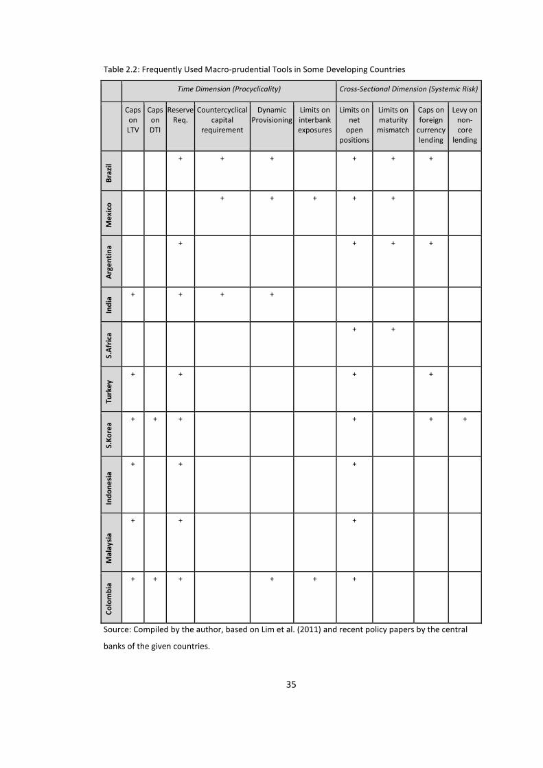
35

Table 2.2: Frequently Used Macro-prudential Tools in Some Developing Countries

Time Dimension (Procyclicality) Cross-Sectional Dimension (Systemic Risk)

Caps on LTV

Caps on DTI

Reserve Req.

Countercyclical capital

requirement

Dynamic Provisioning

Limits on interbank exposures

Limits on net

open positions

Limits on maturity

mismatch

Caps on foreign

currency lending

Levy on non-core

lending

Bra

zil

+ + + + + +

Me

xico

+ + + + +

Arg

en

tin

a + + + +

Ind

ia + + + +

S.A

fric

a + +

Turk

ey

+ + + +

S.K

ore

a

+ + + + + +

Ind

on

esi

a

+ + +

Mal

aysi

a

+ + +

Co

lom

bia

+ + + + + +

Source: Compiled by the author, based on Lim et al. (2011) and recent policy papers by the central

banks of the given countries.

36

demand and term deposits, FX reserve requirements also promote curbing

excessive credit growth. Moreover, foreign exchange reserve requirements also

limits domestic banks’ funding from abroad and supports the tools at the initial

stages of the mechanism. Together with these secondary effects, the main target

of foreign exchange reserve requirements is to control the volatility and the

pressures on the exchange rates.

Apart from the credit and asset markets another implication of financial inflows is

step three, the movements of the exchange rates. When there is an excess level

of financial inflows to a country, appreciation pressures on the exchange rate

tend to rise. In the opposite scenario, the exchange rate faces depreciation

pressures. These pressures generally have significant side-effects over the real

economy, particularly on the current account balance, inflation and real GDP

growth. Rather than buffering reserves, these pressures are aimed to be

weakened by the use of macroprudential tools. As indicated above, foreign

exchange reserve requirements are the more widespread tool to manage the

pressures. Moreover, Turkey introduced a tool called the Reserve Option

Mechanism (ROM) that is designed to control the pressures on the exchange

rate. While foreign exchange reserve requirements are compulsory, the ROM

mechanism is based on voluntarily terms.

Another implication of this step is its connection with the initial step of the path.

There is a strong link between the volatility of capital flows and exchange rates.

The clockwise transmission mechanism can clearly be seen on the cycle. The

volatility in the exchange rate that is mainly due to domestic factors may also

affect the investment decision of foreigners. Tools such as foreign exchange

reserve requirements and ROM are useful in this front also, by blocking the

direct transmission from step 3 to step 1 and vice versa. On one hand, the

volatility in the domestic currency is buffered while, on the other hand, the

volatility of capital inflows is controlled. In both ways, the domestic currency is

supposed to be stabilized and the pressures over the exchange rate are expected

to be lowered. Furthermore, as with the tools in the previous steps, these tools

also have impacts on the rest of the cycle, particularly on financial soundness.

37

Moving along step four, exchange rates and credit/asset markets may fuel each

other in a feedback loop which may at last lead to a further expansion of bank

balance sheets. When there is a significant asset price inflation in an economy,

the demand for credit rises. To provide credit, banks’ reliance for wholesale

funding increases. This cycle leads stretching in banks’ balance sheet and results

in several vulnerability problems in the banking sector. First, since banks often

provide the funding that they seek from outside in foreign exchange, the non-

core liabilities of the banking system tend to increase. A levy on non-core

liabilities aims to curb excessive increases in banks’ non-core liabilities by

reducing arbitrage margin and raising FX funding costs. Moreover, caps on loan-

to-deposit (LTD) ratios are also useful for reducing reliance on wholesale

funding. Secondly, if there is no levy imposed and no appropriate or adequate

measures are taken throughout the mechanism, the financial system most likely

ends up with currency mismatch and maturity mismatch problems, which may

lead bitter results following any shock to the system at any point of the

mechanism. Limits on currency and maturity mismatch may help moderating

these risks. However, these are not time-varying tools and should be backed up

with other ones in the earlier steps of the cycle.

Short-term capital flows are well-known to be subject to sudden stops or

reversals. A volatility of capital flows can be caused by shocks or the mechanism

itself. A change in the global liquidity, global uncertainty or a severe shock in

commodity prices, as well as political instability in the recipient country may

cause volatility in capital flows. Furthermore, an exchange rate misalignment

which proceeds surge of capital inflows may eventually cause volatility of

currency and increase risks for foreign investors. An excess amount of short-

term external debt may also have adverse effects on the foreign investors’

investment decision and cause capital flows to become more volatile.

Instead of limits on maturity and currency mismatches, the tendency of

developing economies after the global financial crisis have been adopting

measures that aim to mitigate the related risks at the initial stages of the path.

To this end, many central banks introduced FX reserve requirements or leverage

caps to limit the excessive leverage to be used for credit funding. Moreover,

minimum holding periods and the tools that can be differentiated according to

38

the maturity such taxes or levies on non-core liabilities aim to mitigate the

maturity related risks at various steps of the mechanism.

The tools explained above mainly address risks during a boom period. However,

there are other countercyclical tools that are defined as ‘automatic stabilizers’,

‘shock absorbers’ or ‘buffers’ that prepares the banks for a downturn and

enhances the resilience of the banking system. Countercyclical capital buffers

and dynamic provisioning are the most widespread ones among those tools. The

former promote banks to raise their capital in the run-up to a boom and lower it

after the bust. Similarly, the latter is the adjustment of banks provisions which

are to be increased during an upswing and decreased in the case of a downturn.

It is important to consider these tools at different stages of the mechanism as a

joint optimization problem. Macroprudential tools may address more than one

risk in the system and the tools may complement each other in mitigating risks.

For example, limits on maturity mismatch addresses credit growth/asset price

inflation, excessive leverage and also have slight effects on capital

flows/currency fluctuation. This emphasizes the importance of forming a well-

functioning policy framework since a simultaneous use of both macroprudential

tools itself and their use along interest rates will be required.

2.5 CHALLENGES FOR IMPLEMENTATION AND THE WAY AHEAD

Despite the consensus on the possible benefits of the use of macroprudential

policy, there are also various concerns upon the challenges of its

implementation. First, the experience with macroprudential policy and literature

on its effectiveness are still limited. Secondly, the joint optimization problem

requires central bankers to develop a well-balanced policy mix which is a hard

and meticulous task. Thirdly, there are still some moral problems upon the

implementation of such tools and there is no consensus on the institutional

framework.

39

Since empirical analysis requires a longer time span, measuring effectiveness of

macroprudential tools have only been possible by assessing the tools that were

adopted by developing countries prior to the crisis. After the financial crisis in the

1990s, developing countries took some macroprudential measures, mainly to

promote the stability of their banking system and to enhance their resilience

against cross-border spillovers. However, in several developing countries

macroprudential measures did not prevent rapid credit growth in the lead-up to

the crisis (Agénor, Pereira da Silva, 2011). In Latin America, for example, credit

growth was accelerating, reaching alarming rates before the crisis (IMF, 2011).

Regarding the post-crisis central banking practices, this can be considered as “a

call for using macroprudential tools more aggressively or for adding new tools to

the arsenal of policymakers” (Agénor, Pereira da Silva, 2011). However, without

solid knowledge on the effects of tools, their selection by central bankers seems

to remain challenging.

As the information and foresight is limited about the effectiveness of

macroprudential policies, it is also a hard task for policymakers to choose the

right combination of instruments. Since interest rates can affect financial stability

and macroprudential tools may have indirect impacts on price stability, the

macro-stabilization exercise must be thought carefully (Eichengreen et al.,

2011). The side effects of each tool must be identified carefully and minimized to

avoid unintended consequences. Macroprudential toolkit must be designed so

that tools would complement each other and therefore the efficacy of the toolkits

would be promoted.

Besides the uncertainty on its effectiveness, there are also some concerns that

extended use of macroprudential policy will lead becoming more subject to

lobbying and political pressure (Agénor, Pereira da Silva, 2011). Higher capital

requirements can bother the agents who had been providing high yields in the

financial sector. Furthermore, adoption of financial stability objective may

adversely affect central bank credibility (Agénor, Pereira da Silva, 2011). Since

there is no consensus yet on how to measure financial stability, there can be

new challenges for the central banks in terms of transparency and

communication of its policy decisions.

40

Lastly, although beyond the scope of this paper, one of the biggest challenges

appears to be institutional arrangements. From the lender of last resort, to the

guardian of price stability, and now having undertaken a mandate to promote

financial stability, much is expected from central banks. At this point, it may be

useful to remember the famous words of Walter Bagehot (1915): “’putting new

wine to old bottles’ is safe only when you watch the condition of the bottle, and

adapt its structure most carefully”. According to the study of Carré (2013)

although the need for the macropudential policy have been accepted by both

central bankers and economists, central bankers' answers reflect their reluctance

on changing the remaining system. There seems to be no consensus on the

structure, whether there should be two units in the central bank to pursue

macroeconomic and financial stability, or central bank can pursue both at the

same time. Some countries formed complementary bodies for monitoring

financial stability, whereas others gave additional responsibilities to central

banks in pursuing this complementary objective. The most common institutional

forms consist of single integrated regulator and twin-peaks model. Nevertheless,

the institutional transformation in many countries still continues.

2.6 CONCLUSION

The global financial crisis led central banking to take a giant step forward in its

evolutionary history. Following the lessons from the crisis, financial stability is

considered as an additional mandate and policy toolkits of central bankers are

expanded with the inclusion of macroprudential policies. These developments

also brought the need to monitor a wider set of indicators. With an expansion

both in the monitored indicators and in the policy tools, the task of central

bankers have turned into a joint optimization problem. For the policymakers of

developing countries, the problem becomes more challenging regarding the

vulnerabilities of these economies against global conditions.

As a first step to overcome this meticulous task, the risks that are faced and the

features of policy tools should be pointed out. In this vein, this Chapter

contributes to the existing literature by identifying risks and introducing a more

41

detailed approach to classify the macroprudential toolkit, while placing

developing countries in its focus. With this method, it is possible to observe how

effective central bankers are in covering the specified risks for a developing

country.

The rest of this study elaborates on some other aspects of this joint optimization

problem. Although there are multiple challenges related to the transformation

process, this study focuses on the first two challenges given earlier: the limited

experience with some macroprudential tools and the meticulous task of central

bankers in developing a well-balanced policy mix. The aim of the two following

chapters is based on the intention to shed light on two issues: the effectiveness

of macroprudential tools and the interaction among the toolkit. While doing so,

the cycle presented in this chapter is used to distinguish the policy mixes in

some selected countries. The next Chapter is designed to assess the

effectiveness of the new policy mixes adopted by some selected developing

countries. The cross-country analysis is beneficial in terms of demonstrating the

effectiveness of certain tools in different economies. Moreover, the common

characteristics of selected countries are also helpful when comparing the tools.

The last Chapter, on the other hand, digs deeper to investigate the tradeoff

within the toolkit. Unlike the previous approaches in the literature, it develops a

new method to measure the effectiveness of the new policy mixes by taking the

interactions of the impact of selected tools into account.

42

CHAPTER 3

POST-CRISIS MONETARY POLICY FRAMEWORKS IN DEVELOPING

COUNTRIES: A CROSS-COUNTRY ANALYSIS ON THE NEW POLICY

MIXES

3.1 OVERVIEW

The previous chapter explains the changes occurring in the understanding of

central banking from the early 2000s to today. The chapter particularly focuses

on the recent developments in central banking after 2008, when the global

financial crisis caused the most drastic punctuation in the equilibrium that had

been observed since the Great Depression. The need for the inclusion of financial

stability in central bank mandates is highlighted. Moreover, special attention is

paid to the emerging consensus on the monetary policy framework that was

shaped upon the lessons from the global financial crisis. This post-crisis

framework came along with multiple implications and challenges: the

introduction or bolstering of macroprudential tools; the interaction of financial

stability and price stability; and the optimal policy choice regarding the joint use

of monetary and macroprudential policy.

The urgency of a new monetary policy framework was emphasized by

international bodies such as the IMF and G20. The adoption of international

regulations such as the Basel requirements was promoted by these bodies.

Despite the international initiatives and co-operations for the promotion of sound

financial systems, there is much more work to do for the central banks of

developing countries. Developing countries, facing a broader set of challenges

regarding their vulnerabilities arising from unsustainable current account deficits,

43

highly volatile exchange rates and capital flows need further measures and

regulations.

In this respect, central banks of many developing countries adopted new policy

mixes that incorporate macroprudential policies in line with the specific risks to

their economies. However, regarding our very little experience with these tools,

we do not yet know where we stand in this “uncharted territory”. The extent of

effectiveness of macroprudential tools, interaction among the tools in the toolkit

as well as the distance taken so far with this new architecture of monetary policy

are almost unknown. Despite an explosion of studies upon the lessons from the

crisis, little attention has been paid to these issues. In line with this need, this

chapter now intends to dig deeper by attempting to assess the effectiveness of

the post-crisis monetary policy frameworks of some important developing

countries.

Three developing countries are selected for this purpose. These are: S.Korea7,

Turkey and Brazil. The selection of countries depends on three important factors.

First, this set of countries can be considered as a fair representation of

developing countries. The GDPs of these three countries form 46% of the total

GDP of the developing countries within G20 (World Economic Outlook, 2014).

Regarding their great potential for future growth and increasing

interconnectedness with the rest of the world, the developments in these

economies should be monitored closely. Secondly, the central banks of these

countries announced their adoption of financial stability as an additional mandate

and explicitly introduced new policy mixes following the global financial crisis. In

this respect, the toolkits and the risks that are addressed are clear. Lastly, their

post-crisis policy mixes form a useful set for a cross-country analysis since they

address similar risks with different macroprudential tools. This enables us to

observe the impacts on different tools on the same objectives.

With such an assessment, this study contributes to the existing literature by

seeking answers to some crucial questions: How do the new policy mixes differ

in the selected countries? Do these differences lead more or less effectiveness?

7 Even though S. Korea has recently started to be considered as a developed country by several

sources, this study takes UN Country Classification Report (2014) into account, where it is classified

as a developing country.

44

If they do, depending on the use of which tools? To this date, there has not been

such an attempt in the literature that focuses on a set of countries for the

assessment of post-crisis monetary policy frameworks.

The findings imply that different choice of tools led different outcomes in

selected countries. The case of S.Korea, in particular, significantly diverges from

the two other cases in several aspects. S.Korean policy mix appear to have

formed a sounder financial system with respect to the other two. Digging deeper,

the cases of Turkey and Brazil also tend to diverge due to different choice of

tools in the capital flow front. The capital flow management tools which were

previously known as capital controls seem to have increased the effectiveness of

the policy mixes in Brazil and S.Korea. However, the most important implication

of the findings is that rather than the choice of certain tools, the design of the

overall policy mix requires more attention. A successfully designed policy mix

should take the interactions among the tools into account.

To provide accurate conclusions upon the effectiveness of the post-crisis policy

mixes, this chapter is structured as follows: The following part presents the new

policy mixes of the three selected developing countries. Their aims and

transmission channels are highlighted. Then, the chapter moves on with the

examination of the literature on measuring the effectiveness of macroprudential

tools. Their scopes, aims and methodologies are presented. In the next part, the

chapter focuses on the assessment of the effectiveness of the post-crisis

monetary policy frameworks of the selected developing countries. The

assessment is conducted by an event analysis, regarding the top variables that

stand out in the literature for indicating overall macroeconomic stability -

financial stability as well as price stability - in conformity with the recent

emerging consensus on central banking. After completing the event analysis and

shaping broad view upon the new monetary policy frameworks’ effectiveness,

the chapter concludes with an overall discussion upon the success of these

frameworks as well as addressing some prospective adjustments.

45

3.2 NEW POLICY MIXES

Figure 3.1 summarizes the details of the new policy mixes utilized by three

selected countries. In Brazil and Turkey, the new policy mixes were introduced in

late 2010, whereas S.Korean policy mix was adopted only a few months before,

in mid-2010. All three policy frameworks consist of tools that cover both credit

and exchange rate related risks. Although the risks that they aim to mitigate are

similar, their toolkits differ significantly.

New Policy Mixes

Adoption Credit Front Exchange Rate/Capital Flows Front

Bra

zil

Late 2010 -Reserve Requirements (RR)

-Restrictions on Consumer Loans

-IOF on Consumer Loans

-IOF on Portfolio Investments by Non-

residents

-IOF on FX Derivatives

-IOF on External Credit Flows

-FX RR

S.K

ore

a

Mid 2010 -Loan-to-Value (LTV) Caps

-Debt-to-Income (DTI) Caps

-Leverage Caps (LC)

-Macroprudential Stability Levy (MSL)

-Taxation of Foreign Bond Investment

-Loan-to-Deposit (LTD) Caps

Turk

ey

Late 2010 -RR

-BRSA measures

-Interest Rate Corridor

-Reserve Option Mechanism (ROM)

-FX RR

Source: Compiled by the Author, based on Central Bank statements, reports, technical notes, etc.

Figure 3.1: Detailed Presentation of the New Policy Mixes of Selected Countries

Curbing the Acceration in Credit

Growth

Controlling Asset Price Inflation

Controlling the Volatility of Capital

Flows and Exchange Rates

Mitigating Currency/Maturity

Mismatch Related Risks

46

Chapter 2 explains the path of capital inflows in developing countries in detail.

Figure 3.2 demonstrates a simplified version of this cycle for each country under

investigation. The outer cycle can be interpreted as the vulnerability of an

economy to global factors, whereas the inner cycle represents the domestic

conditions, particularly the credit cycle. These two cycles have a tendency to fuel

each other or transfer the volatility arisen in a single step to the entire system.

To this end, effective control of each aspect within the cycle is crucial for a

central bank to promote the soundness of the macroeconomic system.

Regarding the excess global liquidity due to the quantitative easing strategies of

advanced countries after the global financial crisis, the primary concern of the

new policy mixes was to limit and/or control the capital inflows. For this purpose,

each central bank adopted measures that address the supply and/or demand-

side factors. Taking the supply-side factors as a point of departure, the list of

measures that are taken are macroprudential stability levy (MSL) in S.Korea,

financial transactions tax (IOF) in Brazil and interest rate corridor in Turkey.

Although discussed to some extent in the previous chapter, it may be useful to

focus more closely on these tools since they can be considered as the

cornerstones of the new policy mixes. While IOF and MSL are measures that aim

to control capital flows by increasing the cost of investment, interest rate

corridor functions by controlling the uncertainty for foreign investors.

Furthermore, IOF and MSL allow authorities to control the maturity of flows by

associating higher rates of charges to short-term flows. Interest rate corridor, on

the other hand, is expected to discourage short-term flows by creating

uncertainty about short-term yields (Aysan et al., 2014). Nevertheless, interest

rate corridor does not necessarily regulate the maturity of capital inflows. Central

Bank of Turkey (CBRT) aims to undertake this task mainly with foreign exchange

reserve requirements (FX RR). FX RR can be differentiated according to maturity

and they may be useful for preventing short-term flows to pass through the

domestic credit cycle. In this respect, effective use of FX RR is supposed to both

save the banking system from maturity mismatch problems and reduce

pressures on the exchange rate. Banco Central do Brazil (BCB), aiming to

mitigate these risks, also introduced FX RR in its new policy mix.

47

Figure 3.2.a: S.Korea

Currency

Mismatch

Maturity

Mismatch

MSL √ √

LC √

LTD √

Figure 3.2.b: Brazil

Currency

Mismatch

Maturity

Mismatch

IOF √ √

FX RR √ √

Figure 3.2.c: Turkey

Currency

Mismatch

Maturity

Mismatch

Int R.C. √ √

ROM √

FX RR √ √

Source: Compiled by the Author

Note: The arrows filled in grey represent the addressed channels by the macroprudential policy

indicated nearby.

Figure 3.2: Macroprudential Tools in Selected Developing Countries

MSL LC

LTV/DTI

LTD

IOF

RR FX RR

RR FX RR

ROM

Interest Rate

Corridor

48

Moreover, regarding the tight two-way relationship between exchange rate and

capital flow volatility, CBRT introduced a new tool – Reserve Option Mechanism

(ROM) – as a part of its new policy mix. As explained in the previous chapter,

this ‘automatic stabilizer’ allows banks to hold a certain fraction of their reserves

in terms of foreign currency. This fraction is called the Reserve Option Coefficient

and can be adjusted by CBRT.

The reserves of banks held within the ROM facility can be released during

stressful times to meet the foreign currency needs of banks. By giving flexibility

to banks in liquidity management, ROM aims to reduce the pressures on the

exchange rate. By doing so, it also aims to contain the transmission of volatility

between exchange rates and capital flows. Another benefit of the ROM

mechanism is further stated by Alper et al. (2012) that with the presence of ROM

accounts, CBRT relies less on direct FX interventions. To this end, the effective

use of ROM is supposed to reduces the need for direct FX purchases and

interventions which in turn minimizes possible undesired communicational

issues.

Another implication of excess capital inflows is the fueling of the domestic credit

cycles. The tools regarding the credit front are listed in Figure 3.1. In Brazil and

Turkey, the primary tool to curb the acceleration of credit growth is reserve

requirements. Additional measures consist of capital requirements and IOF on

consumer loans in Brazil. In Turkey, the Banking Regulation and Supervision

Agency (BRSA) took some tightening measures regarding the credit card

purchases and LTV ratios of vehicle loans, as well as the repayment periods of

several types of consumer loans. S.Korean authorities, on the other hand, focus

on housing price appreciation since early 2000s. Caps on loan-to-value (LTV)

and debt-to-income (DTI) ratios address residential loan growth on wealth and

income aspect respectively.

In a boom phase, banks tend to borrow from abroad. The reliance on wholesale

funding fuels the cycle with currency and maturity mismatch related risks. In this

respect, policy mixes are supposed to cover the demand-side factors too. For

this purpose, BOK adopted caps on loan-to-deposit (LTD) ratio and leverage

caps. The former tool is designed to limit loans to deposits. This way, the tool

49

both promotes financial soundness by improving banks’ liquidity conditions and

reduces the reliance on wholesale funding by preventing undesired expansion in

assets. Leverage caps, on the other hand, are a tool that limits asset growth to

bank equity. It directly affects FX balance sheets and limit banks’ FX borrowings.

Similarly, BCB also addresses the demand channel. An IOF on external credit

flows aims to reduce the reliance on external funding of the Brazilian banking

system. On the other hand, CBRT has not adopted a tool specific to this aspect

of the cycle. CBRT relies on the indirect effects of interest rate corridor, FX RR

and ROM. It is assumed that when domestic banks require further funding, their

reserves held in the ROM facility will enable them to rely less on non-core

funding (Alper et al., 2012).

To fully explain the design of the new policy mixes, the interactions among the

selected tools should be well understood. Each mix has similar aims to be

pursued by different tools. The choice of different tools forms different

interactions that lead benefits or drawbacks for policymakers. To design an

effective policy mix the interactions should be computed carefully. For example,

both ROM and MSL address vulnerabilities that may arise from the banking

sector, from very different aspects. MSL specifically addresses banks’ non-core

liabilities8 and therefore aims to reduce the procyclicality in the banking sector.

Moreover, unlike the examples in other countries such as UK, the proceeds of

the levy are held in a special segregated account of foreign exchange reserves,

called ‘Foreign Exchange Stabilization Fund’ (Bruno and Shin, 2013). In this

respect, MSL may also act as FX RR with regard to its stabilizing effect on the

exchange rate. Since S.Korean policymakers uses leverage caps to control the

FX liquidity that enters into the domestic economy, the interactions seem to

cover the benefits of FX RR without having it included in the toolkit. ROM, on the

other hand, is designed mainly as an automatic stabilizer. Since banks are not

obliged to but voluntarily hold a fraction of their reserves in FX, it significantly

differs from MSL and FX RR. With the use of this tool, CBRT aims to complement

the other tools in the mix - FX RR and interest rate corridor-. When CBRT

changes the FX RR, every bank in the system is obliged to adjust its FX liquidity

accordingly. Therefore, banks with limited access to FX may face difficulties. In

this respect, ROM helps to improve the soundness of the banking system and

8 Foreign exhange denominated liabilities of banks.

50

eliminate possible negative outcomes of the use the FX RR. While doing so, ROM

may also have stabilizing effects on the exchange rate.

However, rather than being a substitute, it stands to be a complement to the

interest rate corridor since their transmission channels differ significantly (Alper

et al., 2012). It is clear that ROM is designed to lower pressures on the

exchange rate through adjusting the use of capital flows received. Unlike ROM,

interest rate corridor aims to stabilize the exchange rate through controlling

investment decisions. To this end, ROM is expected to ease the reliance on the

interest rate corridor to some extent. Moreover, the interest rate corridor has

notable effects on the credit growth front. The credit conditions rely heavily on

the upper bound of the interest rate corridor (Alper et al., 2012). Although all of

the policies mentioned above – FX RR, MSL, leverage caps- have positive effects

in curbing credit growth, these are less direct than the impacts of interest rate

corridor since their transmission mechanism is through the limitation of FX

liquidity. Therefore it is possible to consider the interest rate corridor as an

additional tool for the Turkish toolkit in dealing with the credit cycle. However,

since it is designed to have a transmission channel mainly through managing

investment decisions, the joint optimization should be carefully computed in

order not to suffer from the side effects of certain tools.

IOF, on the other hand, is closer to leverage caps regarding its main

transmission channel. However, unlike leverage caps – which are quantity

based- IOF taxes are priced-based capital flow management tools. In a sense, FX

RR can also be regarded as price-based tools. The opportunity cost of the part of

inflow that is deposited in unremunerated accounts has similar effects with a tax

(Ostry, 2011). In the literature, quantity-based tools are considered to be more

effective than price-based tools. In this respect, the three policy mixes can also

be compared with regard to these features. S.Korean policymakers seem to have

designed a policy mix where quantity-based tools are associated with a larger

weight whereas more importance is attached to price-based tools in Turkish and

Brazilian policy mixes. In Brazil, there appears to be a joint use of the price-

based tools: the FX RR and IOF. As in the Turkish case, Brazilian policymakers

should also take policy interactions into consideration. FX RR is designed to

reduce the pressure on the exchange rate by the deposited amount in the FX

51

reserves. IOF, on the other hand, mainly aims to control the size and maturity

composition of capital flows. Unlike MSL the taxes obtained from the IOF are not

held in a special account. Instead, IOF taxes are converted into local currency.

This may lead pressures on the exchange rate. Hence, these two tools should be

adjusted carefully so that the undesired effects of IOF tax would not offset the

benefits of FX RR on the exchange rate.

When the three policy mixes are evaluated in a broader sense, the capital flow

management measures of BCB and BOK can be interpreted as capital controls

whereas Turkish toolkit seeks to control the cycle in a more market-friendly

manner. Moreover, the Turkish toolkit is narrower in terms of the number of

tools that CBRT relies on. This efficiency may be beneficial for market

communication which is in line with the market-friendly policy choices of CBRT.

Therefore, the effectiveness analysis in the following parts may provide crucial

implications upon these choices. While assessing the effectiveness of the new

framework, the findings can indicate whether the use of tools that are

traditionally known as capital controls is inevitable or it is possible to manage the

cycle without them.

3.3 LITERATURE REVIEW ON EFFECTIVENESS ANALYSIS

There are many studies in the literature assessing the effectiveness of

macroprudential tools, some focusing on certain ones and some on the

aggregate level. These studies also differ among the financial stability indicators

that are investigated and the methodology that they carry out. The most

common methodology is assessing the effectiveness with empirical analysis.

Since the experience of many developing countries with macroprudential tools

date back to early 2000s, the data usually extents to an 8-12 years period of

time. These studies are generally based on a cross-country dataset and focus on

a certain macroprudential tool. Some studies are carried out solely by empirical

analysis whereas some support their empirical work by event analysis. There are

also some studies in the literature that are conducted by event analysis only.

52

Lim et al. (2011), in their cross-country study with a data set of 49 countries for

the period of 2000-2010, use both event analysis and dynamic panel regression

to measure the effectiveness of eight macroprudential policies in limiting the

procyclicality of credit and leverage, and two other macroprudential policies in

reducing systemic risk. They conclude that caps on LTV and DTI, dynamic

provisioning and reserve requirements have been successful in curbing credit

growth. On the other hand, other tools such as caps on FX lending seem to have

had less obvious impacts. Another study conducted by Claessens, Glosh and

Mihet (2012) uses the same panel data set to analyze the effects of

macroprudential policies on banking system vulnerabilities. Both studies explore

the effects of the most commonly used macroprudential policies, but on different

aspects of financial stability and conclude that the policies are effective, at least

under some circumstances. The broad data set consists of developed and

developing countries, both the ones that have adopted macroprudential policy

and the ones that have not, with different policy frameworks and capital account

openness status. The diversity of the data enables them to carry out an

extensive comparison.

On the other hand, the IMF (2012) conducts a study to investigate the

interaction of monetary and macroprudential policies. In this study, they also

assess the effects of macroprudential tools on financial variables such as credits

and asset prices by using cross-country data on the use of macroprudential tools

from 2000 to 2011 in 36 countries. The macroprudential tools that are focused

on are capital requirements, limits on loan-to-value ratios, caps on debt-to-

income and reserve requirements, whereas monetary policy refers to the policy

interest rate. The results from their regression indicate that there is no

significant evidence upon the interaction between monetary and macroprudential

policies, a result verifying the study of Dell'Ariccia et al. (2012). The findings also

reveal that the effectiveness of a macroprudential policy does not depend on the

monetary or FX regime of the country under investigation, in line with the study

of Lim and others (2011). Furthermore, the results from the empirical study

emphasize that reserve requirements are successful in slowing down the credit

growth whereas caps on loan-to-value limits house price appreciation, and

capital requirements are successful in managing both.

53

There are also some country-, and region-specific studies sharing similar aims

with the ones mentioned above. For example, Tovar et al. (2012) analyze the

effectiveness of reserve requirements and other macroprudential policies on

credit growth in Latin America. The event analysis observes the data covering

the period of four months before and after the policy implementation. They

particularly focus on the data on annual credit growth provided to private sector,

policy rates, lending rates and exchange rates. Finding the results of the event

analysis inadequate in terms of not allowing extrication the shocks and the

effectiveness of policies, they complement their analysis with a dynamic panel

data vector auto-regression. The empirical analysis is based on a system

reached by using Generalized Method of Moments. They run the regression over

a vector of a macroprudential policy dummy9, policy interest-rate, level of

economic activity and private bank credit growth; and lags of this vector.

Concluding on the effectiveness of reserve requirements on the slowdown of

credit growth, they underline that “other tools are no less important, but their

role is examined here only tangentially”.

Furthermore, the study of Glocker and Towbin (2012b) explores the Brazilian

experience with reserve requirements by using a bayesian vector auto-

regression model. The model is constructed with a vector of endogenous

variables (unemployment, CPI inflation, current account, Selic rate, reserve

requirements, interest rate spread, loan and central bank reserves) and a vector

of exogenous variables (constant term, trend, dummy for time period, US federal

funds rate, commodity price index). According to the results of the regression,

they find out that reserve requirements complement monetary policy in

promoting financial stability.

In one of the case studies on Korea, Igan and Kang (2012) indicate that caps on

loan-to-value (LTV) and debt-to-income (DTI) limit mortgage credit growth in

Korea. To draw this conclusion, they use data from 2002 to 2010 where they use

an independent variable of interest in housing and mortgage markets, and two

independent variables: a control variable reflecting the general economic

9The macroprudential policy dummy is a cumulative dummy which consists of marginal reserve

requirements, average reserve requirements and private bank credit growth.

54

activity, monetary policy stance and measures of tightness and expectations in

housing markets; and a dummy that reflects the time of any rule change.

The literature puts forward the fact that the studies on measuring the

effectiveness of macroprudential tools generally focus on the tools such as caps

on LTV and DTI, dynamic provisioning and reserve requirements. These tools

stand out to be the ones that were generally adopted by developing and a few

developed countries before the global financial crisis. Thus, the sufficient data

which allows empirical work, is almost only upon these policies.

However, as implied in the previous chapter, together with the changing nature

of central banking, the new monetary policy frameworks have been adopted in

the world after the crisis, mostly in 2010 and 2011. Therefore, the available data

on the new monetary policy frameworks is inadequate for most empirical

approaches and thus the literature on the evaluation of the new monetary policy

frameworks generally relies on event analysis. Empirical studies are generally

conducted in a before-after manner in evaluating the effects of the new

frameworks.

Furthermore, the main implication of the emerging consensus, i.e.

macroprudential policy complementing monetary policy in pursuit of both price

and financial stability, suggests that this new era in central banking needs to be

evaluated differently from the past. Rather than focusing on the success of

certain tools and policies, the new monetary policy frameworks require a broader

assessment of the overall framework since the success of a single tool may have

reversed effects on other indicators due to the interaction between the policies

and objectives.

One example for the assessment of new policy frameworks has been conducted

for Turkey. Kenc et al. (2011) seek evidence from yield curves to show that the

reserve requirements hikes have led a tighter policy stance in Turkey. They also

benefit from event analysis to observe the impacts of the policy framework on

credit and loan growth. Another study (Kara, 2012), also carries out an event

analysis in order to assess the new monetary policy framework of Turkey. This

study, however, takes both financial stability and price stability into account.

55

Kara defines the transmission mechanism from policy tools to both stabilities as

being through the exchange rate and the credits. The study particularly

examines these two variables in assessing the effectiveness of the policies of the

CBRT. The results of the event analysis reveal that, in the financial stability side,

there was a slowdown in credit growth and an amelioration in the exchange rate

volatility relative to other developing economies at the end of 2011, after a year

that the new policy framework was adopted. On the other hand, pointing at the

significant deviation from the official inflation target at the last quarter of 2011,

Kara (2012) concludes that the CBRT policies haven't been that successful in the

price stability front.

Similar to the study of Kara, Pereira da Silva and Harris (2012) assess the

effectiveness of the new policy mix in Brazil by observing the changes in related

data. They also evaluate the toolkit based on the two transmission channels:

exchange rate channel and credit channel. Their analysis reveals that IOF and

other complementary tools have been effective in reducing the rate of carry

trade and lengthening the maturity composition of external loans. Moreover, the

study asserts that credit-related measures have also been successful by curbing

the growth of credit to a more sustainable pace.

Studies on Brazil focus more on the tools related to capital flow management.

Chamon and Garcia (2014) conduct an empirical analysis on the post-crisis

measures in Brazil. They conclude that capital flow management measures in

Brazil, particularly IOF have been effective in increasing the cost of domestic

assets for foreign investors. The effectiveness of Brazilian measures is also

pointed out in other studies. Baumann and Gallagher (2012) find evidence of an

amelioration in the maturity composition of capital inflows and reduced exchange

rate volatility after the introduction of the new policy mix. Furthermore, Forbes

et al. (2011) conclude that portfolio flows have been reduced. Jinjarak et al.

(2013), on the other hand, find out that the IOF measures do not have any

significant impact on the magnitude of capital inflows, instead there have been a

moderation in the magnitude of outflows during stressful times. Earlier studies

on the effectiveness of capital controls also drive some similar results. Binici et

al. (2009) put forward that debt and equity controls are successful in reducing

outflows whereas limited impact is observed on the volume of capital inflows.

56

Similarly, the studies of both Magud et al. (2011) and Ostry et al. (2010) reveal

that capital controls have positive impacts on the composition of flows, but

limited effects on the volume of flows.

Regarding its huge reliance on the external factors before and during the global

financial crisis, studies on Korean economy generally evaluate the performance

of the new policy mix in terms of its resilience on global risk factors. Ree et al.

(2012) conduct such a study focusing on the two well-known vulnerabilities of

the Korean financial system: currency mismatch and exchange rate volatility.

Their findings reveal that a significant reduction of Korean short-term external

debt weakened the link between exchange rate volatility and global risk factors

(proxied by VIX). Therefore, they assert that the resilience of Korean financial

system to external shocks have remarkably been reduced after the global

financial crisis. The empirical study of Bruno and Shin (2013), also reach similar

findings. They deal with 48 countries including Korea, and find out that after

2010 -the year which Korean authorities announced the adoption of new

macroprudential tools- Korea's sensitivity to global factors decreased, whereas

the findings draw an image in the opposite direction for other East Asian

countries, particularly the Big Five10. Furthermore, other studies focused on

Korea indicate that the new monetary policy framework of Korea has been

successful. The macroprudential levy, caps on loan-to-deposit and ceilings on

banks FX derivative positions are “effective in curbing banks' reliance on short

term FX funding and in reducing vulnerabilities from FX mismatches and

exchange rate volatility” (Bruno and Shin, 2012). A recent study of Baumann

and Gallagher (2013), however, finds limited evidence on the effectiveness of

the S.Korean capital flow management measures on exchange rate appreciation

and volatility.

Aysan et al. (2014) follow a similar strategy to Bruno and Shin (2013) in order

to assess the sensitivity of Turkish financial system to global factors. They use a

panel regression specification with a dependent variable of banking sector capital

inflows and an independent variable of the growth of interoffice assets of foreign

banks in US. The independent variable stands as a proxy for the rate at which

global banks are engaged in wholesale funding to the rest of the world. They

10

Indonesia, Malaysia, Philippines, Thailand and Vietnam.

57

also include the VIX variable that reflects the leverage of global banks and a

control variable as independent variables. The results reflect that capital flows to

Turkey has become less sensitive to cross-border global banking activities after

the implementation of the new monetary policy framework with macroprudential

policies.

3.4 ASSESSING THE EFFECTIVENESS OF THE POST-CRISIS MONETARY

POLICY FRAMEWORKS IN THE SELECTED DEVELOPING

COUNTRIES

The literature review shows that a vast majority of relevant studies are only

concerned with the effectiveness of certain macroprudential tools. They do not

possess the intention of assessing the effects of an overall monetary policy

framework. Furthermore, a limited number of studies being carried out with this

intention, focus only on a single country. The importance of this study is that this

section investigates the post-crisis monetary policy frameworks of a set of

developing countries, trying to figure out how effective they have been so far.

The similarities and differences of the three toolkits may enable us to draw some

conclusions on the characteristics of a correct policy toolkit for developing

countries. As far as the literature review indicates, the related literature does not

elaborate on an assessment with such a concern.

In order to provide such conclusions, this section assesses the effectiveness of

the post-crisis monetary policy frameworks of selected developing countries by

examining the trend of the available data on the countries’ macroeconomic and

financial systems. Indicators are examined regarding the time of the adoption

and adjustments of macroprudential measures. While conducting this analysis,

the study benefits from the indicators used both in the literature for similar aims

and in the financial stability or economic activity reports of central banks. Even

though the event analysis approach does not provide a deep examination in

terms of indicating comprehensive conclusions or extrication of the effects of

policies from shocks, it may still serve as a useful way to shape a broad view

58

over the effects of policies. Since the new policy frameworks address both

financial stability and price stability, the examination will concern both fronts.

It was already mentioned in the previous chapter that there is no absolute

consensus on which indicators should financial stability can be observed.

However, there are two main transmission channels addressed in the design of

the new policy mixes: capital flows /exchange rate and credit channels.

Therefore this section is structured to focus on these two transmission channels

closely. Lastly, the overall effects on the macroeconomic system and financial

soundness are examined.

3.4.1 Volatility of Capital Flows and Exchange Rate

After the global financial crisis, the primary concern of the central bankers of

developing economies has been to limit and regulate the surge of capital inflows

in order to prevent procyclicality. The procyclical behavior generally starts with

large surges of capital flows and causes vulnerabilities in financial and

macroeconomic stability. Excess capital inflows lead appreciation pressures on

domestic currency and worsen current account balance on one hand, while on

the other hand they fuel the domestic credit cycle by providing excess liquidity to

banks. Stretching bank balance sheets may encourage non-core funding11 and

cause further vulnerabilities. To this end, controlling maturity composition and

magnitude of capital inflows is crucial for developing economies.

11

Funding through FX denominated liabilities.

59

Source: IMF BOPS Statistics

Figure 3.3: Net Capital Inflows over GDP in Selected Developing Countries12

12

Financial derivatives and employee stock options form a significant part of flows only in S.Korea.

In Brazil and Turkey the share of the given category is negligible. Thus, the figures for Turkey and

Brazil do not include financial derivatives.

-3,50%

-2,50%

-1,50%

-0,50%

0,50%

1,50%

Figure 3.3.a: S.Korea

Fin. Acct., Fin. derivatives(other than reserves) andemployee stock optionsFin. Acct., Other invest.

Fin. Acct., Portfolio invest.

Fin. Acct., Direct invest.

-2,00%

-1,50%

-1,00%

-0,50%

0,00%

0,50%

1,00%

1,50%

2,00%

Figure 3.3.b: Brazil

Fin. Acct., Portfolio invest.

Fin. Acct., Other invest.

Fin. Acct., Direct invest.

-1,50%

-1,00%

-0,50%

0,00%

0,50%

1,00%

1,50%

2,00%

2,50%

Figure 3.3.c: Turkey

Fin. Acct., Other invest.

Fin. Acct., Portfolio invest.

Fin. Acct., Direct invest.

60

Figure 3.3 shows the vulnerability of capital inflows to global factors. All of the

three countries experienced large capital reversals during the peak of the global

financial crisis. There are several factors that may make an economy to be more

subject to such volatility of capital flows. These factors generally include large

external debts and unsustainable current account deficits for most of the

developing countries. The countries under investigation in this section suffer

from one or both of these factors which required them to adopt appropriate

measures after the global financial crisis.

Table 3.1: Coefficient of Variations for Gross Financial Inflows

From 2006 to late

2010

From late 2010 until

2015

All Period

Brazil 71% 25% 51%

S.Korea 139% 91% 136%

Turkey 85% 43% 66%

Table 3.1 shows the volatility of gross financial inflows for selected developing

countries. The coefficient of variation values indicate that the volatility of

financial inflows was higher before the new policy mixes were in effect. The

coefficient of variation values have been significantly reduced for all of the

countries, at varying rates. The different levels of amelioration in the volatility of

financial flows address the impacts of different policies that were put in effect.

Hence, a separate analysis for each policy mix is required.

In late 2010, Central Bank of Republic of Turkey (CBRT) introduced interest rate

corridor to manage the volatility of capital flows. Regarding the excess surge of

capital flows at the time of its introduction, the lower bound was cut and the

corridor was widened. The uncertainty promoted by the corridor discouraged

foreign flows. In late 2011 and early 2012, the Eurozone debt crisis intensified

and the rise of the global uncertainty implied volatility of capital flows. In

response, CBRT increased the upper bound to attract capital inflows. In the late

2012 and early 2013, the global uncertainty declined and CBRT again responded

61

with a decrease of the upper bound. Figure 3.3.c shows that the active use of

the interest rate corridor may have helped the volatility of capital inflows to

decline with respect to the pre-crisis period. However, in mid-2013, following the

US Fed announcement of tapering policy, capital inflows declined. Although CBRT

increased the upper bound and cut the lower bound in late 2013, Turkish

economy could not avoid a gradual decline in capital inflows.

Despite being successful in managing the capital flows during a period of

volatility, interest rate corridor became no longer effective after the economy

faced a larger shock in 2013. Furthermore, although interest rate corridor aims

to prevent excessive short-term flows by its nature, it does not necessarily

regulate the composition of flows. Figure 3.5 shows the share of short-term

foreign debt within gross external debt in three countries. While the Turkish

measures only incorporate foreign exchange reserve requirements, the tools that

are used for this purpose are numerous in other countries. CBRT’s first response

to the accelerating rate of short-term foreign debt was to increase foreign

exchange reserve requirements. In November 2010, the foreign exchange

reserve requirements were increased from 9 to 11. A few months later, CBRT

made an adjustment in foreign exchange reserve requirements according to

maturities so that short-term deposits were associated with the highest ratio.

Figure 3.5.c shows that following the implementation of these measures, the rise

in the short-term debt ratio slowed down until the end of 2011. However, a

gradual rise followed, from the beginning of 2012. Although CBRT cut the upper

bound and pulled the lower bound to discourage capital inflows, surges persisted

until the second half of 2013. Both gross external debt and the share of short-

term debt rose steadily (Figure 3.4, Figure 3.5.c). There appears to be a two-

way causality. When evaluated with the decline of short-term financial flows

shown in Figure 3.3.c, the slowdown in the rise of short-term foreign debt is

more likely to be associated with global factors rather than being under control

of CBRT.

Furthermore, the failure of interest rate corridor may have been caused by the

large accumulation of short-term foreign debt until 2013. Figure 3.4 shows that

Turkey had the largest external debt to GDP ratio among three selected

countries in 2013. Furthermore, Figure 3.5.c demonstrates that almost 35% of

62

this debt was with short-term maturity. Together with the uncertainty due to

Fed’s tapering policy, this large ratio may have discouraged international flows to

a larger extent than in the other selected countries.

Source: WorldBank, UNStats

Figure 3.4: Gross External Debt in Selected Countries

In fact, before the crisis hit developing countries, the short-term to total external

debt ratios of Turkey and Brazil were almost at the same level, around 17%.

However, after the introduction of new policy mixes, the ratios of the two

economies diverged significantly. In this respect, it may be useful to compare

the macroprudential tools implemented by CBRT and Banco Central do Brasil

(BCB).

BCB also responded its rising short-term external debt by increasing foreign

exchange reserve requirements. Introduced in January 2011 at a rate of 60%,

this tool particularly addressed short-term deposits. It remained in effect until

the second half of 2013. Unlike CBRT who only relied on the interest rate

corridor, BCB complemented its measures with several types of the financial

transactions tax- IOF- within this time frame. The first type of IOF is on portfolio

investments by non-residents, aiming to discourage carry trades in spot and

future markets. In March 2011, BCB introduced a second IOF measure on

external credit inflows. Moreover, a third type of IOF was introduced in July 2011

on FX derivatives. These set of measures seem to have helped Brazilian short-

term debt to decrease from 17% of GDP in late 2010 to 8% in late 2012.

63

When the Turkish and Brazilian cases are compared, it is clear that foreign

exchange reserve requirements are a useful tool to control the magnitude and

maturity of FX denominated debt and therefore the FX liquidity in the market.

However, the experiences under investigation reflect that this tool should be

complemented with more direct tools such as taxes or caps. The Korean example

reinforces this argument.

Source: CBRT, BCB, BOK

Figure 3.5: Short-term Foreign Debt in Selected Developing Countries

64

Before the global financial crisis, when Brazilian and Turkish short-term to total

external debt ratios were approximately around 17%, the data on Korean

economy reflected a ratio over 50%. In line with the possible vulnerabilities that

such ratio may cause, S.Korean economy faced the sharpest capital flow reversal

among the three selected economies during the peak of the crisis (Figure 3.3.a).

Accordingly, Table 3.1 clearly shows that the volatility of financial flows to

S.Korea have been the highest among three selected countries. Moreover, Figure

3.3.a also demonstrates that unlike in Brazil and Turkey, S.Korean financial

outflows offset financial inflows. This case is particularly persistent since the

beginning of 2012. There are several reasons for these distinguishing features of

the Korean financial system. First, Korean capital account openness is the

highest among the selected countries. As Ree et al. (2012) also indicate in their

study, the Korean capital account openness is placed at the top end of emerging

market economies by the Investment Freedom Index (Wall Street Journal,

Heritage Foundation) and even at the top end of the world by the Capital Access

Index (Milken Institute). Furthermore, during Great Moderation years, when the

S.Korean economy was receiving large capital inflow surges, authorities took

several measures to promote outflows (Kim, 2012). These measures succeeded

in making residents’ investments overseas to offset foreign capital inflows

(Figure 3.3.a). Lastly, S.Korean external borrowing was mainly driven by the

demand of exporters- particularly shipbuilders- for FX hedging. The expectations

of further appreciation of the Korean Won formed a cyclical lending behavior and

contributed the build-up of a large external debt, which is mainly composed of

non-core liabilities of banks. In this respect, before the introduction of its new

policy mix in mid-2010, the immediate response of Bank of Korea (BOK) after

the crisis was to introduce loan-to-deposit (LTD) caps. Introduced in December

2009, LTD caps aim to reduce the procyclicality of bank lending behavior by

limiting banks’ reliance on wholesale funding.

The BOK then announced its adoption of a set of measures in mid-2010. In

October 2010, when financial flows to developing countries had been increasing

in a worrisome manner, Korean authorities introduced caps on FX derivative

positions and leverage caps in order to curb banks’ short-term external debt.

These measures were actively used by tightening for several times. The new

policy mix also addressed the bond market with the reintroduction of the tax on

65

foreign investors’ bond investment. In August 2011, BOK adopted

macroprudential stability levy on non-core liabilities of the banks. The levy

implies a charge on foreign currency denominated liabilities of banks up to 12

months of maturity whereas maturities of over one year are associated with

lower rates (Bruno and Shin, 2013). In this respect, the macroprudential stability

levy aims to mitigate the risks arising from both maturity and mismatch

problems (effects on related indicators are given later). The levy has further

stabilizing effects since the charge from banks are held as foreign exchange

reserves in order to be released at stressful times. After the implementation of

these tools the short-term external debt ratio declined to a range of 30% of GDP

in 2013 and 2014. While gross external debt to GDP remained almost constant

as of late 2010, short-term over total external debt declined steadily. This

asserts that the maturity composition of Korean debt have been significantly

ameliorated proceeding the introduction of the new policy mix.

Source: BIS

Figure 3.6: Effective Exchange Rates in Developing Countries

The tools listed above also aim to control the volatility of exchange rates.

Controlling the risks that are associated with capital flows automatically provides

central banks to reduce the pressures on domestic currencies. The large capital

surges after crisis led appreciation pressures on the domestic currencies of

66

developing countries after the global financial crisis. Figure 3.6 shows the

exchange rate movements in the three selected countries with respect to the

average of developing countries.

After the introduction of the new policy mix in November 2010, Turkish lira

recorded a significant depreciation of 20% in less than a year (Figure 3.6). The

policy mix proves to have helped reducing the appreciation pressures on

domestic currency during a period of large capital flow surges. In September

2011, CBRT complemented its toolkit with an additional tool. As indicated

previously, Reserve Option Mechanism (ROM) was announced as an automatic

stabilizer and a market-friendly tool. It allows banks to hold a certain fraction

(determined by the reserve option coefficient) of their required reserves in

foreign currency or gold. This way, banks accumulate foreign exchange reserves

during large capital flow surges which are to be released in a case of capital

outflow. Therefore, the pressures on domestic currency can be lowered.

Although introduced in the second half of 2011, Alper et al. (2012) note that it

was in June 2012 when the tool became fully in effect. Accordingly, Figure 3.8

demonstrates that the official reserve assets recorded a noticeable increase

proceeding this date.

Source: IMF, WorldBank

Figure 3.7: International Reserves as % of Gross External Debt

67

The overall policy mix seems to have successfully reduced the risk of volatility of

Turkish lira during a period of global uncertainty due to the European debt crisis.

Turkish lira stands to be relatively more stable among others from late 2011 to

mid-2013 (Figure 3.8). This fact is highlighted in the studies of Aysan et al.

(2014) and Alper et al. (2013). The latter put forward that although CBRT did

not engage in direct FX interventions since the beginning of 2012, Turkish lira

remained stable throughout the year. However, with the Fed announcement of

tapering policy, the bright picture upon Turkish lira diminished. Figure 3.6 shows

that TL faced a notable depreciation of 20% while the developing countries’

average was approximately 10%. While Turkish lira was experiencing this

gradual depreciation, Brazilian real depreciated at a rate closer to the developing

countries average. Starting from May 2013- when Fed announced its possible

tapering policy- Turkish lira depreciated by 17% within a year. Brazilian Real, on

the other hand, depreciated much moderately by 6%. Within the same time

frame, Korean Won significantly diverged from other developing country

currencies with a 9% appreciation.

Although Brazilian exchange rate appears to have had responded to this shock

more moderately, the story underneath reveals some different implications on

the success of BCB. The framework of BCB indicated that IOF is supposed to

stabilize the currency by regulating the capital flows. Simple reasoning asserts

that when the maturity composition of capital flows is fixed, the pressures on the

exchange rate should be lowered. However, IOF may have other side effects on

the exchange rates as indicated in the earlier section where the policy mixes are

presented. IOF measures were introduced in period when no further appreciation

in the exchange rate was desired. By limiting capital inflows, IOF should have

helped a fair depreciation in the exchange rate. However, Figure 3.6 shows that

a significant appreciation occurred after the introduction of the new policy mix.

Although FX RR at a rate of 60% was introduced in 2011, the depreciation only

took place in late 2011 when the Eurozone debt crisis intensified. Moreover, in

early 2012 another IOF regulation took place mainly aiming to regulate the

maturity composition of capital inflows. However, through mid-2012, both capital

inflows shrank and exchange rate depreciated. Together with inflationary

concerns and low output levels in 2012, as well as the increasing current account

68

Source: BIS Exchange Rate Data

Note: The range in grey represents the volatility interval (+/- 2 st. deviations of the median) for

developing countries within G20. The mean for the interval calculation is based on 3 months moving

average standard deviation.

Figure 3.8: Volatilities of Selected Domestic Currencies

deficit and a large reduction in the Selic rate, further depreciation became

undesirable. Therefore, an initial response of BCB was to attract more capital

inflows by loosening of its IOF measures by the end of 2012. In 2013, IOF taxes

on fixed income and derivatives were eliminated. Starting from late 2013, Brazil

managed to attract more capital inflows. However, a joint observation of Figure

3.7 and 3.8 reveals that these policy adjustments were not effective in the

exchange rate front, since the relatively more stable trend in Brazilian Real in

the second half of 2012 was managed along with a large reduction in the

reserves. With the elimination of some of the IOF measures by early 2013, even

the relatively stable path of Real – controlled with interventions – no longer

existed.

69

Source: Alper et al. (2013)

Figure 3.9: ROM Utilization Rate

Focusing on the Turkish case, indicators demonstrate that CBRT started to lose

its control over capital inflows starting from 2012. Although the effects of this

loss of control were not clear in the exchange rate front during 2012, it became

obvious on various aspects of the financial and macroeconomic system after the

Fed announcement of tapering policy in 2013. It was already stated with the

ROM facility becoming in effect, the international reserves of CBRT increased

remarkably due to the rise of reserve holdings in the ROM accounts. However,

Figure 3.9 indicates that this facility hasn’t been used in a large scale during

periods of capital outflows. Therefore, the ROM may not have been used by

banks in the way that CBRT expects. Aslaner et al. (2014) explain this

ineffectiveness by the side effects of the use of the interest rate corridor on the

ROM facility. They assert that when there is an increase in the interest rates to

attract capital inflows, the cost of Turkish lira funding increases and it becomes

more profitable for banks to use ROM. To this end, the automatic stabilizer

feature of ROM becomes weakened. Accordingly, the volatility of Turkish Lira,

which was significantly dampened during 2012, worsened after mid-2013 with a

sharp depreciation.

While Turkish and Brazilian policymakers are trying to lessen the depreciation

pressures on their exchange rates in the past couple of years, the challenge of

S.Korea have been remarkably different. The Korean Won adopted a divergent

trend from the rest of the developing countries since mid-2012 and diverged in a

broader sense since the announcement of US tapering policy. The starting date

FX ROM Utilization in Turkey (percent)

70

of this divergent trend is in conformity with the Figure 3.3.c earlier, which

addresses the same date for S.Korean investments abroad significantly offsetting

the foreign capital inflows. The same date can also be distinguished from Figure

3.8 as the start of an increase in the reserve accumulation. Moreover, Figure 3.6

shows that in line with the gradual decline in the short-term external debt, the

resilience of Korean Won to external factors has risen. From the introduction of

the policy mix in mid-2010 to the date of Fed announcement of tapering policy in

mid-2013, Korean Won remained in a +/- 5% range of appreciation or

depreciation whereas the Turkish and Brazilian currencies experienced a

depreciation up to 20%. It is also clearly seen from Figure 3.8 that the Korean

Won remains as the most stable currency among the selected currencies.

While the Won remains relatively stable, after mid-2013, it started to appreciate

at a rate which is more than desired. During the Great Moderation years, BOK

saw such upswings as a threat to the export sector since the appreciation may

undermine the sector by weakening profitability. In 2013, the governor of Bank

of Korea, Kim Cehoong-soo said that the exchange rate should be left in the

market fundamentals, implying that they let the currency to appreciate. He also

added that the appreciation of Won would have moderate impacts on exports

since the export industry is now driven by goods based on advance technology.

From mid-2013 to mid-2014, the Won recorded an appreciation of 15% with a

significant risk for the Korean economy. In mid-2014 another interview was

given by the Governer Lee-Ju-yeol implying that the large current account

surplus leads some worries that the currency is bound to appreciate, along with

the increase in the current account surplus. A current account surplus may have

been a source of buffer against the global causes of domestic volatility. However,

a further reliance on this buffer may have led some concerns since the export-

oriented manufacturing industry remains as the cornerstone of the economic

growth in S.Korea. Therefore, a stable, but also a competitive exchange rate is

the essential policy goal of the authorities to maintain economic growth

(Leiteritz, 2014).

Another implication from the moderate volatility of Won is that BOK managed to

control the feedback loop between the volatility of capital flows and exchange

rate. The volatility of financial flows did not pass through the exchange rate

71

front. This successful barrier forms a supporting example for the discussion in

the previous section. The MSL may have acted as FX RR in restraining the FX

liquidity entering into the market by holding the excess FX in the Foreign

Exchange Stabilization Fund. Moreover, the rise in the current account surplus

(to be discussed further later in the Chapter) and large international reserves

(Figure 3.8 earlier) also should have contributed to the fall of volatility in the

exchange rate front.

3.4.2 Acceleration of Credit Growth and Asset Price Inflation

As discussed before, advanced countries followed quantitative easing strategies

after the crisis, which led an excess global liquidity. Unless appropriate measures

are taken, this global liquidity ends up in an acceleration of credit growth in

developing countries through surges of capital inflows. The control over credit

growth is important for the financial system as a whole, since banks tend to seek

foreign funding during the upswings, which may fuel foreign debt as well as

causing currency and/or maturity mismatch problems. If not managed properly,

episodes of excessive credit growth may lead to growing imbalances and tend to

end abruptly (Elekdag and Wu, 2011).

Figure 3.10 show that the selected countries experienced significant increases in

their credit to GDP ratios both before and after the global financial crisis.

Although the acceleration of credit was widespread among developing countries,

each economy has different driving forces behind its credit growth. In this

respect, central banks of developing countries adopted measures to curb the

credit growth both on the aggregate level and by addressing specific types of

loans.

72

Source: BIS

Figure 3.10: Credit in Selected Developing Countries

Figure 3.11 shows that the composition of household loans in S.Korea, Brazil and

Turkey. The mortgage loans forms around 61% of total loans on average in

S.Korea whereas their share among Turkish household loan form 42% of total

loans. The different composition of loans brings different challenges for

economies. While Korean credit related measures mostly cover the housing

sector, Turkish measures focus on other loans, particularly consumer loans.

While the share of mortgage loans among total loans remained almost stable in

Turkey and S.Korea for the period under investigation, Figure 3.11.c shows that

the ratio in Brazil followed an upward trend. Mortgage loans that formed 13% of

total loans in early 2008, reached 22% in early 2011 and 36% in early 2014.

Unlike S.Korea, the policy mix of Brazil have not specifically addressed the

housing sector, but aimed to curb the credit growth in an aggregate level. As will

be discussed later, the lack of policies addressing the housing sector is due to

the fact that the expansion of mortgage loans in Brazil does not only depend on

cyclical factors but also structural changes occurred towards the housing sector.

73

Source: BOK, IMF FSI Database, CBRT

Figure 3.11: Loan Composition in S.Korean and Turkish Banking Systems

In Turkey and Brazil, the primary tools to curb the accelerating credit growth

have been reserve requirements. BCB and CBRT also took additional measures

regarding the specific features of their loan compositions. Figure 3.12

demonstrates the movement of credit growth along with the measures taken.

Figure 3.11.a: Mortgage and Other Loans over GDP in S.Korea

Figure 3.11.b: Mortgage and Other Loans over GDP in Brazil

Figure 3.11.c: Mortgage and Other Loans over GDP in Turkey

74

After BCB adopted its new policy mix in late 2010, credit growth started to follow

a downward trend. BCB promoted this downward trend with the simultaneous

rise of reserve requirements and Selic rate until the second half of 2011. These

measures were also complemented with the increase of capital requirements on

consumer loans in December 2010. The Risk Weight Factor was increased for

consumer loans mainly for vehicle financing (which accounted for 25% of

outstanding household loans in December 2010) and consumer credit. This

measure did not include mortgage loans (Pereira da Silva and Harris, 2012).

Moreover, an IOF tax on consumer credit was introduced in April 2011. This set

of measures helped BCB to curb the credit growth from a rate of 24% in January

2011 to 18% in January 2012. In November 2011, when the credit growth first

reached the rate of 18%, Luiz Pereira from BCB stated that the credit growth

had slowed down to a sustainable pace. After that point, to avoid any further

slowdown in the growth rate The Risk Weight Factor and Selic Rate were lowered

in the second half of 2011 while reserve requirements were held constant.

However, the growth rate slowed down further to almost 15% in late 2012.

Another statement from BCB followed, declaring that “there is still room for

credit to expand further and that would be desirable”. Despite a notable cut in

the RRs and elimination of some IOF measures, credit growth continued to slow

down towards rates below 15% throughout 2013, simultaneously with the rise in

the Selic rate which was in fact adjusted to attract capital flows after the Fed

tapering talk. In this respect, although the Brazilian policy mix was successful in

curbing the credit growth, it fell short when policymakers started to seek further

expansion in credit.

CBRT also took several measures to address the acceleration of credit growth.

CBRT increased the reserve requirements substantially at several steps from

November 2010 to April 2011 and tightened the interest rate corridor by cutting

the lower bound in August 2011. Another measure followed the set of tools to

curb the accelerating credit growth in mid-2011. Regarding the large share of

consumer loans in this acceleration, Banking Regulation and Supervision Agency

(BRSA) took several measures. These included several types of limitations to the

monthly spending with credit cards. Furthermore, capital requirements for

consumer loans were raised. Figure 3.12.b clearly indicates that these measures

75

Source: BCB, CBRT

* Year-over-year.

Figure 3.12: Credit Growth in Selected Developing Countries

had been notably successful in curbing the credit growth after August 2011. In

conformity with the adjustments in the interest rate corridor, the decline in the

credit growth rate continued until late 2012. After 2012, CBRT remained

reluctant to use reserve requirements actively. The movements of credit growth

rate in 2013 and 2014 have been mainly associated with another episode of

BRSA measures and the interest rate corridor. In November 2013, BRSA

announced a new set of limitations to credit card purchases and the introduction

of LTV caps on vehicle loans. Furthermore, the repayment periods for vehicle

and housing loans were limited to 48 and 36 months respectively. Around the

same date, the interest rate corridor was also aggressively adjusted upwards in

0%

5%

10%

15%

20%

25%

30%

6

8

10

12

14

16

18

11

-20

10

02

-20

11

05

-20

11

08

-20

11

11

-20

11

02

-20

12

05

-20

12

08

-20

12

11

-20

12

02

-20

13

05

-20

13

08

-20

13

11

-20

13

02

-20

14

05

-20

14

08

-20

14

11

-20

14

Figure 3.12.a: Credit Growth in Brazil (y-o-y)*

Selic Rate

RR (weightedaverage)

CreditGrowth(Total) -rightaxisCreditGrowth(Households)-right axis

0%

5%

10%

15%

20%

25%

30%

35%

40%

45%

50%

0

2

4

6

8

10

12

14

11

-20

10

01

-20

11

03

-20

11

05

-20

11

07

-20

11

09

-20

11

11

-20

11

01

-20

12

03

-20

12

05

-20

12

07

-20

12

09

-20

12

11

-20

12

01

-20

13

03

-20

13

05

-20

13

07

-20

13

09

-20

13

11

-20

13

01

-20

14

03

-20

14

05

-20

14

07

-20

14

09

-20

14

11

-20

14

Figure 3.12.b: Credit Growth in Turkey (y-o-y)

Interest RateCorridor

RR (weightedaverage)

CreditGrowth(Total) - rightaxis

CreditGrowth(Households)-right axis

76

order to encourage capital flows, after the Fed tapering talk. As a result of these

policies the credit growth rate approached to more desired levels recently. The

set of BRSA measures can be seen as an exceptional attempt to promote

financial stability with regard to the “market-friendly” toolkit of CBRT. The policy

coordination between these two bodies appears to be successful in curbing the

undesired acceleration in the consumer credit front.

The credit growth performances of the countries under investigation reveal that

both central banks face different policy dilemmas. In Turkey, credit growth

seems to be in a negatively correlated co-movement with the upper bound of the

interest rate corridor. A significant decrease in the upper bound triggers an

undesired credit growth for CBRT. On the other hand, in Brazil, while a rise in

the Selic rate leads contraction in the credit growth, a cut does not seem to be

able to help fuel the growth rate through desired levels. Evidence from the above

analysis assert that a more active use of macroprudential tools that are not

directly related with interest rates may help central banks avoid such policy

dilemmas arising from the multilateral impacts of interest rates. When interest

rate related policies are implemented for attraction or limitation of capital flows,

the credit growth rates are affected too. Therefore, when the impact of the

interest rate related tool is negative with regard to the targets of central banks,

the use of other tools should be expanded. This is clearly seen from the Turkish

example in Figure 3.12.b that if Turkish authorities could have used reserve

requirements more aggressively in early 2013, credit growth might not have

risen back at a rate of 35% and could be curbed before the actions of BRSA and

an increase in the interest rate corridor.

A greater credit supply is associated with asset price inflation (Brunnermeier et

al., 2012; Borio and Disyatat, 2011). Regarding the acceleration of credit

growth, another concern of developing countries is the risk of a housing bubble

with residential price appreciation and high mortgage loan growth. Garber

(2000) defines a housing bubble as the part of the housing price movement that

cannot be explained by the fundamentals. On the other hand Shiller and Case

(2003) suggest that this term refers to a situation which excessive public

expectations for future price increases cause prices to be temporarily elevated.

More specifically, according to Mayer (2011) when housing prices rise rapidly,

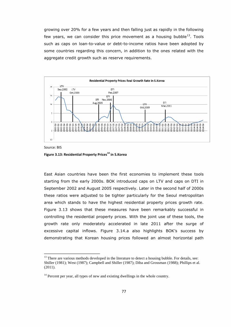
77

growing over 20% for a few years and then falling just as rapidly in the following

few years, we can consider this price movement as a housing bubble13. Tools

such as caps on loan-to-value or debt-to-income ratios have been adopted by

some countries regarding this concern, in addition to the ones related with the

aggregate credit growth such as reserve requirements.

Source: BIS

Figure 3.13: Residential Property Prices14

in S.Korea

East Asian countries have been the first economies to implement these tools

starting from the early 2000s. BOK introduced caps on LTV and caps on DTI in

September 2002 and August 2005 respectively. Later in the second half of 2000s

these ratios were adjusted to be tighter particularly for the Seoul metropolitan

area which stands to have the highest residential property prices growth rate.

Figure 3.13 shows that these measures have been remarkably successful in

controlling the residential property prices. With the joint use of these tools, the

growth rate only moderately accelerated in late 2011 after the surge of

excessive capital inflows. Figure 3.14.a also highlights BOK’s success by

demonstrating that Korean housing prices followed an almost horizontal path

13

There are various methods developed in the literature to detect a housing bubble. For details, see:

Shiller (1981); West (1987); Campbell and Shiller (1987); Diba and Grossman (1988); Phillips et al.

(2011).

14

Percent per year, all types of new and existing dwellings in the whole country.

78

after the crisis. Considering the upward trend in developing countries’ average,

BOK has been remarkably successful in controlling the housing prices.

On the other hand, in Brazil, where the signs of a “housing bubble” appeared

through early 2010, the residential property prices recorded the sharpest

upswing. Residential property prices increased by over 20% in real terms, from

early 2010 to mid-2012. The average appreciation rate in developing countries

was less than 10% for the same period (Figure 3.3.14.a). However, as implied

earlier, the fact that BCB have not adopted any measures regarding the

persistent upswing in the housing sector is due to the structural changes aiming

to expand the housing market rather than an ignorance. As Figure 3.11.b shows,

the share of mortgage loans among total loans provided to households was

around 13%, which is remarkably low with respect to other emerging market

economies. After various legal and structural changes15, Brazilians who had

stayed away from the housing market for decades, have started accessing the

housing market (Pereira da Silva and Harris, 2012). In line with these

encouragements for access, BCB also addressed in a statement given in late

2012 that the desired driving force for credit growth expansion is the housing

sector. After mid-2012, the appreciation of Brazilian residential property prices

almost stopped while the developing country average continued an appreciating

trend. Figure 3.14.c also demonstrates the diminishing rate of growth in

residential property prices in Brazil. The stable prices may have occurred due to

the measures of BCB on both capital inflows and credit growth front as well as a

slowdown in the demand after the first reaction to the structural and legal

changes.

However, as also indicated in this section earlier, the share of residential real

estate loan in total loans is still rising persistently (Figure 3.14.b). This may lead

further appreciation in the housing prices and increase in credit growth in the

near future as desired by BCB.

15

Some of the changes are a new mechanism called “alienação fiduciária” and the Law 109331/04

that amended the Civil Code. For details, see Pereira da Silva and Harris (2012).

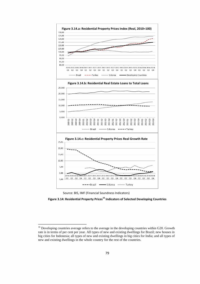
79

Source: BIS, IMF (Financial Soundness Indicators)

Figure 3.14: Residential Property Prices16

Indicators of Selected Developing Countries

16

Developing countries average refers to the average in the developing countries within G20. Growth

rate is in terms of per cent per year. All types of new and existing dwellings for Brazil; new houses in

big cities for Indonesia; all types of new and existing dwellings in big cities for India; and all types of

new and existing dwellings in the whole country for the rest of the countries.

Figure 3.14.a: Residential Property Prices Index (Real, 2010=100)

Figure 3.14.b: Residential Real Estate Loans to Total Loans

Figure 3.14.c: Residential Property Prices Real Growth Rate

80

In Turkey, although the share of residential property loans in total loans remain

almost constant (Figure 3.14.b), residential property prices index show a

persistent upswing (Figure 3.14.a). Mainly after early 2013, the rise in the prices

is above the average in developing countries. Figure 3.14.c also demonstrates

that the movements in the growth rate highly match with the developments in

the capital flows. The growth rate declines following the times when capital flows

wane –in late 2011 when Eurozone debt crisis intensify and in the second half of

2013 after the tapering talk – and rises during surges of capital inflows. Given

this volatility which addresses a sensitivity of domestic conditions to external

factors, the developments in the Turkish housing sector may require closer

attention.

In this light of the above discussions, the analysis on the housing sector implies

that both Brazilian and Turkish indicators seem to be under control for the time

being. However, if the upswing in the indicators persist and reach levels more

than desired, additional measures such as the ones in East Asia may be required

to be adopted.

3.4.3 Overall Effects of the Policy Mixes on Financial Stability and Price

Stability

Figure 3.15 shows financial flows and current account deficits in Brazil and

Turkey. Although the Brazilian current account deficit widened from 2% of GDP

in 2010 to 3.38% in 2013 (IMF, 2014), FDI flows have also followed an upward

trend. This indicates that the measures of BCB to regulate the financial flow

composition have been successful. The maturity of flows has lengthened and the

current account deficit is almost entirely financed by long-term flows. This

implies a narrowing of risks in the Brazilian financial system and less exposure to

the impacts of global factors.

On the other hand, in Turkey, the majority of capital flows to finance the current

account deficit are short-term flows. Although there had been a moderate

amelioration in the magnitude of FDI flows after the introduction of new policy

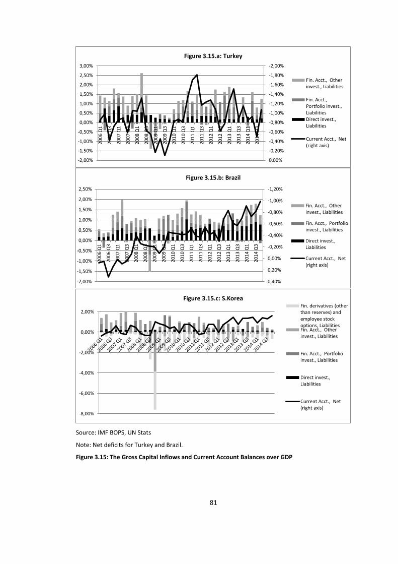
81

Source: IMF BOPS, UN Stats

Note: Net deficits for Turkey and Brazil.

Figure 3.15: The Gross Capital Inflows and Current Account Balances over GDP

-2,00%

-1,80%

-1,60%

-1,40%

-1,20%

-1,00%

-0,80%

-0,60%

-0,40%

-0,20%

0,00%-2,00%

-1,50%

-1,00%

-0,50%

0,00%

0,50%

1,00%

1,50%

2,00%

2,50%

3,00%

20

06 Q

1

20

06 Q

3

20

07 Q

1

20

07 Q

3

20

08 Q

1

20

08 Q

3

20

09 Q

1

20

09 Q

3

20

10 Q

1

20

10 Q

3

20

11 Q

1

20

11 Q

3

20

12 Q

1

20

12 Q

3

20

13 Q

1

20

13 Q

3

20

14 Q

1

20

14 Q

3

Figure 3.15.a: Turkey

Fin. Acct., Otherinvest., Liabilities

Fin. Acct.,Portfolio invest.,LiabilitiesDirect invest.,Liabilities

Current Acct., Net(right axis)

-1,20%

-1,00%

-0,80%

-0,60%

-0,40%

-0,20%

0,00%

0,20%

0,40%-2,00%

-1,50%

-1,00%

-0,50%

0,00%

0,50%

1,00%

1,50%

2,00%

2,50%

20

06 Q

1

20

06 Q

3

20

07 Q

1

20

07 Q

3

20

08 Q

1

20

08 Q

3

20

09 Q

1

20

09 Q

3

20

10 Q

1

20

10 Q

3

20

11 Q

1

20

11 Q

3

20

12 Q

1

20

12 Q

3

20

13 Q

1

20

13 Q

3

20

14 Q

1

20

14 Q

3

Figure 3.15.b: Brazil

Fin. Acct., Otherinvest., Liabilities

Fin. Acct., Portfolioinvest., Liabilities

Direct invest.,Liabilities

Current Acct., Net(right axis)

-8,00%

-6,00%

-4,00%

-2,00%

0,00%

2,00%

Figure 3.15.c: S.Korea Fin. derivatives (otherthan reserves) andemployee stockoptions, LiabilitiesFin. Acct., Otherinvest., Liabilities

Fin. Acct., Portfolioinvest., Liabilities

Direct invest.,Liabilities

Current Acct., Net(right axis)

82

mix, this trend did not last long. The share of FDI flows among other financial

flows to finance the current account deficit worsened after mid-2012. Moreover,

the composition of flows has also been deteriorated with respect to the pre-crisis

period. Relying on short-term financial flows to finance its current account

deficit, Turkish financial system and macro-economy possess a higher

dependence on global factors than the Brazilian example.

Proceeding the worsening of the financial flow composition in Turkey, the

indicators of currency and maturity mismatch have also been at alarming rates

for the past couple of years (Figure 3.16.c). The rate of net open position in

foreign exchange and the ratio of liquid assets to short-term liabilities of the

Turkish banking system worsened rapidly after 2012. Regarding the analysis in

the previous parts, this deterioration is likely to be picturing the unintended

results of the increase of short-term external debt in 2012 and the loss of control

of CBRT on the management of capital flows in after 2012.

Brazil, on the other hand, seems to have fixed the maturity and currency

mismatch problems of its financial system significantly. As discussed in the

previous sections, IOF measures have helped the decline of short-term external

debt and have reduced the vulnerabilities of Brazilian economy to external

factors. These developments are reflected in the balance sheets of banks with a

lag.

S.Korean indicators also show similar results to those of Brazil. Figure 3.16.a

demonstrates that the measures of BOK have especially been successful in

lengthening the maturities of bank liabilities. Since the primary concern of

policymakers in S.Korea has been the rate of non-core liabilities, these indicators

reflect the success of the policy mix of BOK.

83

Source: Financial Soundness Indicators, IMF

Figure 3.16: Indicators for Currency and Maturity Mismatch in Selected Developing Countries

84

Source: IMF BOPS Database

Figure 3.17: Investment Income in Selected Countries

-16,000

-14,000

-12,000

-10,000

-8,000

-6,000

-4,000

-2,000

0,000

2005Q1

2005Q4

2006Q3

2007Q2

2008Q1

2008Q4

2009Q3

2010Q2

2011Q1

2011Q4

2012Q3

2013Q2

2014Q1

2014Q4

Bill

ion

s

Figure 3.17.a: Investment Income in Brazil

Invest. Income, Direct Invest., Net Invest. Income, Portfolio invest., NetInvest. Income, Other invest., Net

-3,500

-3,000

-2,500

-2,000

-1,500

-1,000

-0,500

0,000

0,500

2005Q1

2005Q3

2006Q1

2006Q3

2007Q1

2007Q3

2008Q1

2008Q3

2009Q1

2009Q3

2010Q1

2010Q3

2011Q1

2011Q3

2012Q1

2012Q3

2013Q1

2013Q3

2014Q1

2014Q3

Bill

ion

s

Figure 3.17.b: Investment Income in Turkey

Invest. Income, Direct Invest., Net Invest. Income, Portfolio invest., NetInvest. Income, Other invest., Net

-10,000

-5,000

0,000

5,000

10,000

15,000

20,000

25,000

30,000

-6,000

-4,000

-2,000

0,000

2,000

4,000

6,000

2006Q1

2006Q3

2007Q1

2007Q3

2008Q1

2008Q3

2009Q1

2009Q3

2010Q1

2010Q3

2011Q1

2011Q3

2012Q1

2012Q3

2013Q1

2013Q3

2014Q1

2014Q3

Bill

ion

s

Bill

ion

s

Figure 3.17.c: Investment Income and Current Account Surplus in S.Korea

Invest. Income, Direct Invest., Net Invest. Income, Portfolio invest., Net

Invest. Income, Other invest., Net Current Acct., Net (right axis)

85

Although S.Korean indicators reveal positive implications upon its financial

fundamentals, there is an underlying problem for the future performance of the

economy. Figure 3.16 earlier shows that there is a persistent increase in the

current account surplus of the country. It is already stated in the earlier sections

that S.Korean authorities are not pleased with this rise. Although the S.Korean

economy have been experiencing net financial outflows recently, the level of the

surplus continues to rise, which implies that there should be other factors

underneath. Figure 3.17 shows the net investment income levels in the countries

under investigation. While the net investment income levels are negative in

Turkey and Brazil, Figure 3.17.c indicates that S.Korea has been receiving a

significant investment income since late 2011. It is clearly observable that the

persistent rise in the current account surplus follows the switch of the net

investment income to positive. Taking this into account one can conclude that

the income of residents from their investments abroad has significantly

contributed the rise in the current account surplus. Therefore, although some

positive impacts of these developments are observed in terms of lowering the

volatility of some indicators in response to global factors, the policies of

S.Korean authorities in mid-2000s to promote capital outflows might have

caused a new chain of problems for the Korean economy.

Source: UNStats

Note: HCPI for Turkey, CPI for the rest of the countries

Figure 3.18: CPIs of Selected Developing Countries

86

Figure 3.18 show that developing countries have not shown a good performance

on the price stability front, as of the date of introduction of the new policy mixes.

Similar to financial stability, price stability have also been affected by global

factors. The quantitative easing strategies of US FED in late 2008 caused

inflationary pressures in 2009 and 2010. In late 2011 and early 2012, the

European debt crisis intensified and caused a contraction in the world economy.

World economic growth declined to 3,2% in 2012 from a rate of 3,9% in 2011.

The decline of global demand also caused subdued inflationary pressures on

developing countries by reducing export levels. To this end, 2012 was a year of

lower growth and reduced inflationary pressures for developing countries. In

2013, although the effects of Eurozone crisis lessened, the announcement of US

FED tapering policy in May 2013, put depreciation pressures on domestic

currencies and stimulated inflationary pressures on economies. On the growth

side, advanced countries performed better than developing countries, causing

further capital outflows. Moreover, declining commodity prices caused additional

challenges for commodity exporters.

Turkey, after introducing new monetary policy framework in late 2010, recorded

an inflation rate of 10,5% in 2011, which is dramatically above the official target

of 5,5%. Despite attaining a rate within the uncertainty band in 2012, the rates

in 2013 and 2014 exceeded the upper band. Although the depreciation pressures

of 2013 and 2014 caused the Brazilian inflation rate also to rise, the inflation

rates in Brazil remained within the tolerance intervals. However, since the

tolerance interval of +/-2pp provide a notably wide range to target for the

authorities, these realized rates do not necessarily imply a very successful

performance of BCB on the price stability front.

S.Korea, on the other hand, maintaining the lowest point target of 3%, achieved

to realize inflation rates that fall within the tolerance interval of +/-1pp in 2011

and 2012. However, S.Korean economy faced dramatically low inflation rates

around 1,3% in 2013 and 2014, falling far behind the lower bound of the

tolerance interval.

87

Figure 3.19: Inflation Targets and Realized Inflation in Selected Developing Countries

While Brazil and Turkey faced increasing inflation rates during 2013 and 2014,

the Korean rates followed an opposite trend. These opposite movement are in

conformity with the appreciation trend of Korean Won, which accelerated

especially after mid-2013. Furthermore, the residents’ investments abroad

offsetting the foreign capital inflows, the divergence of the Won with respect to

other developing countries’ currencies and the first significant fall in the inflation

rate address 2012 as a turning point for the Korean economy. In this respect, it

is possible to conclude that even though the rise in the current account surplus

and the accumulation of large international reserves act as a buffer against

global shocks, the impacts of these measures in the macroeconomic front started

to become worrisome. The policy mix of S.Korea seems to have achieved its goal

in terms of promoting a sounder financial system. Nevertheless, the slow-down

in the real GDP growth and inflation rates requires more attention of the

policymakers in these fronts.

88

Source: OECD Statistics

Note: Growth rate compared to the same quarter of previous year, seasonally adjusted

Figure 3.20: GDP Growth Rates in Selected Developing Countries

Figure 3.20 shows that S.Korean GDP growth rate fell behind of those of Brazil

and Turkey. The relatively similar patterns among three cases started to

differentiate for the case of S.Korea, mainly after 2013. Before that date, the

Turkish GDP growth rate appears to be fluctuating sharply and revealing a

remarkably higher rate during 2011, with respect to the other countries. This

performance may have occurred due to the market-friendly strategies as well as

the sharp decline of the given rate in response to the global financial crisis.

Starting from 2012, Turkish growth rate moves along with the Brazilian growth

rate, remaining behind 5%. In this respect, although Turkish policymakers

enjoyed relatively better GDP growth rates on average after the global financial

crisis, the rate started to follow the same trend as in the other two cases after

2012. In S.Korea, the notable decline after the given year may have occurred

due to the sharp appreciation trend as indicated before.

As in the case with GDP growth rates, Turkish indicators followed a fluctuating

trend in the case of another ultimate target, unemployment rates. Turkish

unemployment rate have been by far the highest among the three selected

countries after the crisis (Figure 3.21). The rate recorded the sharpest upswing

during 2009 that it also experienced the most remarkable decline during 2010

and 2011. S.Korean unemployment rate remained almost stable while a

downward trend is observed in Brazil. The downward trend in the Brazilian

unemployment rate continued until 2014, whereas the Turkish rate switched to

89

an upward trend after the tapering talk. When considered altogether, one might

conclude that the Turkish economy have been hit by the impacts of the tapering

talk more significantly than the Brazilian economy. The results in the ultimate

targets front support the previous findings in terms of indicating that the

Brazilian economy has become less dependent on global factors after the global

financial crisis.

Source: OECD Statistics

Figure 3.21: Total Unemployment Rates in Selected Developing Countries

3.5 CONCLUSION

The analysis conducted in this chapter reveals important results on both the

effectiveness of certain macroprudential tools and the new policy mixes of the

selected developing countries. In line with the general view in the literature,

reserve requirements stand to be effective in curbing the credit growth.

Moreover, the analysis also demonstrates that caps on LTV and DTI are

successful tools in dealing with accelerating mortgage loans and housing prices

appreciation. Other policies such as capital requirements in Brazil and BRSA

measures in Turkey also appear to be effective in controlling the acceleration in

the credit growth.

While the tools in the credit front provide more straightforward conclusions, the

tools in the exchange rate/capital flows front are harder to draw conclusions on.

90

For example, while FX RR in Turkey have been initially effective at the time of its

introduction, its effects are less obvious in the proceeding periods. Brazilian FX

RR, on the other hand, has ambiguous effects on the Brazilian exchange rate and

the analysis particularly asserts that the impacts of this tool on the exchange

rate front could have been offset by the side effects of IOF measures. Therefore,

unlike some studies given in the literature review, the event analysis reveal no

significant findings of positive impacts of the new policy mix on the exchange

rate volatility front.

Nevertheless, in terms of dealing with the maturity composition of capital flows,

IOF measures reflect a successful record. The new policy mix seem to have had

a significant positive impact on the composition of the flows and very limited or

no impact on the magnitude of inflows. In this respect, the findings of the event

analysis are consistent with the conclusions of Jinjarak et al. (2013) and the

earlier literature on the effectiveness of the capital controls.

Examined together with S.Korean capital flow management measures, the

attempt to place capital flows management measures have helped both Brazil

and S.Korea to ameliorate their currency and maturity mismatch problems. Their

short-term external debt declined remarkably after the introduction of their new

policy mixes. Although the volatility of financial inflows to S.Korea remains

relatively high, the BOK has been significantly successful in controlling the

volatility of Won. This success may be due to the indirect stabilizing effects of its

capital flow management measures, particularly MSL. Despite the fact that

S.Korean authorities do not incorporate tools such as FX RR or ROM that directly

address the exchange rate front, it seems as a successful policy design brought

the most stable currency among the ones under investigation. The large current

account surplus and international reserves are other significant factors

contributing to the success of BOK in controlling the volatility of the domestic

currency. Taking these points into consideration, the analysis shows that

S.Korean indicators seem to be less dependent on global factors, in line with the

relevant literature.

In Turkey, where market-friendly policy choices are in place, the short-term

external debt has been steadily increasing. The effects of the new policy mix

91

were only initially observable. Moreover, the ROM facility seems to have helped a

significant reserve accumulation to take place after becoming fully in effect at

the first half of 2012. However, there are no significant findings which show that

banks benefited from their reserves held within the ROM facility in the periods

when capital inflows wane. This supports the findings of Aslaner et al. (2014)

that the use of interest rate corridor to attract more flows during stressful times,

may have lead banks to consider the high interest rates as an opportunity rather

than benefiting from their reserves in the ROM accounts.

The analysis in this chapter also provides implications for the selected countries

in terms of some possible adjustments or prospective tools to be included in

their policy mixes. For the case of Turkey, interest rate corridor almost proves to

fall short in regulating the maturity of capital inflows, leaving the risks ongoing

throughout the system. The fact that it may also have negatively affected the

functioning of ROM reinforces the case against the implementation of interest

rate corridor in the current manner. Since the undesired interaction of these two

tools is more likely to take place when there is a reversal in portfolio flows, a

measure which would specifically regulate these types of flows could both ease

the pressures on the interest rate corridor and mitigate the side-effects arising

from its joint use with ROM.

In the Brazilian policy mix, the major problem is the control of the pressures on

the exchange rate. Since the maturity composition of capital inflows have

successfully been managed, the case for the side effects of IOF taxes on

exchange rate reinforces. A possible suggestion for the solution of this problem

could be a more active use of the existing tools. From the time of their adoption

to elimination, the FX RR and several types of IOF were not adjusted.

Considering the large fall in the reserves after the Brazilian Real took a

depreciation trend, another suggestion could be that the adoption of ROM

facility. Such a policy could help BCB to intervene the FX market less frequently.

Moreover, although the Brazilian and Korean capital flow management

frameworks stand to be more effective than the Turkish market-friendly policy

mix, they also have had some costs. The Brazilian authorities could not manage

to accelerate the credit growth to the levels that they had desired. Furthermore,

92

both Korean and Brazilian real GDP growth rates fall behind the Turkish rate17.

The case of S.Korea has its own distinguishing features as stated throughout the

Chapter. However, it seems likely that Brazilian credit and GDP indicators may

have suffered from the distortionary effects of capital controls to some extent.

Another important finding is that mid-2012 has been the date for divergence of

the three sample countries. The individual problems of each economy arose

around this date. BCB lost its control over the exchange rate front. Its efforts to

keep the currency stable along with a significant reduction in international

reserves failed and the domestic currency depreciated sharply. The volatility of

the Real could also not been managed. Around the same date, S.Korean

authorities faced a problem of a persistently increasing current account surplus

heavily due to the received investment income from abroad. The international

reserves started to rise along with the sharp appreciation in Won. Inflation

remained below the target and GDP growth fell behind the desired rates. Almost

at the same date for the start of the chain of problems faced by BCB and BOK,

the success of CBRT started to weaken too. CBRT started loose its control over

the short-term external debt in mid-2012. This loss of control has many

implications since it means the maintenance on the dependence of the economy

on the external factors. Combined with a large current account deficit, the short-

term external debt stock resulted in serious maturity and currency mismatch

problems. The efforts to make the Turkish Lira stable failed which became

apparent after the tapering talk. Moreover, in addition to these multiple

vulnerabilities, inflation dampened remarkably. It should be noted that although

the findings upon the Turkish case do not reveal a bright picture, they do not

necessarily conflict with the relevant literature too. The time frame that is

covered in earlier analyses does not extend to the time frame of this study.

Considering the given chain of events in the countries under investigation, it is

possible to see examples which verify the fueling cycle given at the beginning of

this chapter.

It is also possible to detect some possible future challenges for the selected

economies from this analysis. For the case of Korea, it is already stated earlier

17

The rates are: 3,22 for Brazil; 3,74 for Korea and; 5,44 for Turkey on average for the years from

2010 to 2014 (based on data from WorldBank).

93

that the current picture in the current account surplus started to raise some

concerns for the policymakers. The recent efforts of BOK have been large cuts in

the policy rates to ameliorate the levels of GDP, inflation and other indicators

that may cause concerns for the export based growth model of Korea. Although

these efforts may moderate the current situation, a balanced policy is needed. It

should be taken into account that the current approach to cut interest rates may

fuel the historical problems of the Korean economy with household debt and

housing sector, unless appropriate measures are taken. For Brazil, it seems as

the distortionary effects of capital controls may further constrain credit growth

and GDP. The recent rise in the Selic rate may also worsen this situation. The

joint optimization should be managed meticulously so that BCB would not face a

future policy dilemma. Unlike Brazil and Korea, the possible future issues for

Turkey may arise from the currency and maturity mismatch problems, driven by

its large short-term external debt. Neglecting financial soundness may lead

undesired impacts on the entire financial and macroeconomic system.

In fact, besides the conclusions on the effectiveness of macroprudential tools,

the main implication of this chapter has been the importance of the joint

optimization problem that central bankers should deal with. The analysis shows

that rather than the choice of certain tool, the choice of the framework requires

more attention. The cases with MSL, IOF and ROM form examples for the

situations where the indirect effects of tools can either facilitate the task of

central banks by supporting each other or make it more difficult by limiting the

effectiveness of another by showing some side-effects.

Although this chapter contributes to the existing literature by pointing out the

problematic outcomes of the new policy mixes and suggesting some prospective

solutions them, there is still much to do. With the event analysis approach, we

can see the impacts of the tools on the primary indicators that they are designed

to address. However, although this chapter makes moderate attempts, the

indirect effects of each tool on different indicators should also be observable in

order to conduct a comprehensive analysis on the effectiveness of the new policy

mixes. The limited experience with the new policy mixes and the unknown

indirect effects of newly developed tools make this era of central banking

practices rather an “uncharted territory”. To this end, the next chapter aims to

94

carry out such a comprehensive analysis by developing a new method. This new

method should be able to demonstrate the extent of effectiveness of a policy mix

while also taking the interactions into account.

95

CHAPTER 4

ASSESSING POST-CRISIS MONETARY POLICY FRAMEWORKS

WITH A CENTRAL BANKING EFFECTIVENESS INDEX: A COMPASS

FOR THE UNCHARTED TERRITORY

4.1 OVERVIEW

Lessons from the global financial crisis brought a remarkable change in the

understanding of central banking. It was understood that financial stability

should have counted more than a second-order issue and the overall

macroeconomic stability could not be promoted without pursuing financial

stability in addition to the price stability. Indeed, the inclusion of financial

stability in central banking objectives led the requirement of additional tools for

central bankers, who were operating almost only through controlling short-term

interest rates a few years ago. Most developed and developing countries started

or bolstered the use of macroprudential tools. Therefore, as well as their control

panels the toolkits of central bankers were also expanded. Regarding the limited

experience with such tools, these developments have caused new struggles for

economists and central bankers in pursuit of conducting effective monetary

policy and its monitoring. Despite an explosion of studies conducted recently on

this area, this “uncharted territory” still requires further focus.

After this gradual change, the former ways of monitoring the effectiveness of

monetary policy are also no longer valid. An additional objective and new policy

tools, all in interaction with each other form a difficult task for central bankers

and economists to conduct a comprehensive assessment. In other words, the

96

previous approaches for assessment require an “update” for this new era of

central banking.

Nevertheless, unlike with price stability, the indicators over which the financial

stability could be monitored are rather vague. Furthermore, a vast majority of

the studies regarding this aim are conducted for developed countries. For

developing countries, the studies are mostly country-specific. Regarding this

need, this study seeks a way to assess and analyze the new path of central

banking practices in selected developing countries.

The countries under investigation are Brazil and Turkey. They are both within

G20 economies and the “Fragile Five”. Moreover, the previous Chapter

demonstrates that Turkish and Brazilian economies show remarkably similar

patterns in their economies, in terms of the risks they face with and the

measures that they adopt. They both face large current account deficits,

inflationary pressures and risks arising from large capital flows. Although the

macroprudential tools that were adopted to address their domestic credit cycles

are similar, their measures against the undesired results of capital flows differ.

Chapter 3 deeply examines the policies that are implemented in these countries

and their effectiveness in terms of achieving desired rates and levels for the

indicators that they monitor. However, the event analysis approach does not

allow a comprehensive assessment and only provides partial information.

Following such approach, monitoring the interactions between policies and

indicators is only possible with the intuitive support. Therefore, event analysis

mostly allows making conclusions upon the effectiveness of certain tools and a

comparison between similar tools that are implemented to address the same

indicators in the economy, rather than a comprehensive assessment of the

overall effectiveness of the monetary policy frameworks.

This study aims to investigate the effectiveness of the pre- and post-crisis

monetary policy frameworks by forming a Central Banking Effectiveness Index

for selected developing countries. The uniqueness of this approach is that former

studies with similar purposes were conducted mostly by empirical or event

analysis. There are indices constructed with the aim of informing about the

monetary stance. However, these take the previous consensus on monetary

97

policy into account. Moreover, information upon the monetary stance can only

form one side of the effectiveness analysis. This study undertakes a harder task

by not only being concerned with the monetary stance in the new era in central

banking but also assessing the extent of its effectiveness. It was mentioned

above that considering the limited experience with macroprudential tools and the

scarcity of research about the effectiveness of post-crisis monetary policy

frameworks, the new era in central banking practices is rather an “uncharted

territory”. In this respect, the Central Banking Effectiveness Index is designed to

be an appropriate “compass” by providing crucial information about the success

of the central banks of the countries under investigation, that have developed or

in the course of developing policies to deal with this “uncharted territory”.

The Chapter is organized as follows. Section II presents the frequently used

indices in the literature and summarizes the relevant work for the purpose of this

study. Special attention is paid to the financial stability indicators that should be

incorporated when assessing for developing economies. While doing so, their

scope, aim, methodology and contributions to the existing literature are

discussed. Next, in the light of the literature review, section III moves on with

the construction of the Central Banking Responsiveness Index step by step.

Definitions of selected indicators, description of the data and methodology are

presented. The Central Banking Effectiveness Index is formed following the same

methodology. The last section demonstrates the findings of the analysis that is

carried out with the indices that are developed in the previous section and draws

conclusions upon the success of the pre- and post-crisis monetary frameworks

both in a country-based and a cross-country-based manner.

4.2 LITERATURE REVIEW ON INDICES

Indices are frequently used tools in conducting quantitative analysis where

empirical data and event analysis cannot provide sufficient information. In this

study, since the post-crisis monetary policy frameworks do not provide us the

required data time frame to conduct an accurate empirical assessment, the aim

is to investigate the impacts of the emerging consensus on central banking

98

practices by constructing an index. In order to form a correct index and examine

its possible implications, this section first explores the previous indices in the

literature and provides a background for the formation of the Central Banking

Effectiveness Index. The indices that shed light on the way of constructing the

central banking effectiveness index are: the trilemma indices (monetary

independence index, exchange rate stability index and capital account openness

index), monetary conditions indices, financial conditions indices, aggregate

financial stability indices and some other indices related to the stress of the

financial or banking system. Moreover, the section also provides information on

how central banks decide upon their policies and which variables are observed

for this aim. Early warning indicators, financial stability indicators and their

relevance for the index construction will also be examined throughout this

section.

Figure 4.1: The Impossible Trinity

floating exchange rate regime must give up its monetary independence (Figure

4.1). For each trilemma aspect, an index has been formed:

The monetary independence index (MI), which is developed by Aizenman, Ito

and Chinn (2012), is the reciprocal of the annual correlation of the monthly

Trilemma measures are based on the three

corners of the concept “the impossible

trinity”. The three corners are: exchange

rate flexibility, monetary independence and

capital account openness. The trilemma

implies that these three macroeconomic

policy goals cannot be reached at the same

time. In other words, for example, a

country with full financial integration and a Exchange Rate Stability

99

interest rates between the home country and the base country. The formula is

constructed so that the values vary within the range of [0,1]18:

MI = 𝟏 − 𝒄𝒐𝒓𝒓(𝒊𝒊,𝒊𝒋)+𝟏

𝟐

where 𝑖𝑡 and 𝑖𝑗 represent the home country and base country interest rates

respectively. A higher value indicates higher degree of monetary independence.

On the other hand, regarding the second policy goal of the trilemma concept, the

exchange rate stability index (ERS) is constructed by Aizenman, Ito and Chinn

(2012). It assesses the exchange rate stability by calculating the annual

standard deviations of the monthly exchange rate between the home country

and the base country. By construction, the values computed by the index range

within [0,1] and the highest value indicates the greatest degree of exchange rate

stability. The formula for ERS is as follows:

ERS = 𝟎.𝟎𝟏

𝟎.𝟎𝟏+𝒔𝒕𝒅𝒆𝒗(𝜟(𝐥𝐨𝐠(𝒆𝒙𝒄𝒉_𝒓𝒂𝒕𝒆))

To measure the extent of exchange rate flexibility, a majority of the rest of the

literature addresses two indices based on the idea of exchange market pressure

(EMP). The theoretical foundation for EMP stems for a basic monetary model

incorporating the demand for money, its supply and relative PPP (Cavoli and

Rajan, 2006)19. The usual equation for EMP is as follows:

18

In the construction of the MI index, authors benefit from the following formula for transforming the

values that are within [-1,1] to [1,0]: 𝑪. [𝒙−𝑨

𝑩−𝑨] + D. [𝟏 −

𝒙−𝑨

𝑩−𝑨] where values of x within the range

[A,B] are transformed to be within the range [C,D] .

19

For details, see: Girton and Roper, 1977; Tanner, 2001; Pentecost et al. 2001, Guimaeres and

Karacadag, 2004).

100

𝐸𝑀𝑃1= 𝛥e −∆𝑓

With the use of this equation, the level of exchange rate flexibility is determined

regarding the relationship between the change in exchange rates (𝛥e) and

change in foreign reserves (∆𝑓). There are also two alternate index forms to

measure exhange rate flexibility.

𝐸𝑀𝑃2= 𝜎𝐸𝑅 𝜎𝐸𝑅 + 𝜎𝑁𝐹𝐴⁄

𝐸𝑀𝑃3= 𝜎𝐸𝑅 𝜎𝐸𝑅 + 𝜎𝑁𝐹𝐴 + 𝜎𝐼𝑅⁄

where 𝜎𝐸𝑅 is the annual standard deviation of monthly percentage difference in

the exchange rate, 𝜎𝑁𝐹𝐴 is the annual standard deviation of monthly percentage

difference in reserves and 𝜎𝐼𝑅 is the annual standard deviation of monthly first

differences in money market rates. 𝐸𝑀𝑃2 only takes reserve interventions into

account whereas 𝐸𝑀𝑃3captures both reserve and interest rate interventions. By

construction, values from both indices range from 0 to 1. For determining the

associated weights, some studies use theory (Girton and Roper, 1977) whereas

some others use empirical models (Pentecost et al, 2001).

On the other hand, there are many indices developed in the literature pursuing

the aim of measuring financial openness. Quinn et al. (2011) classify these

various measures into two categories: de facto and de jure indicators. De facto

indicators can be quantity-based, price-based or hybrid measures.

A quantity based measure is the index developed by Lane and Milesi-Ferretti

(2003). They use the following ratio to measure financial integration:

𝐼𝐹𝐼𝐺𝐷𝑃𝑖,𝑡 = (𝐹𝐴𝑖,𝑡+ 𝐹𝐿𝑖,𝑡)

𝐺𝐷𝑃𝑖,𝑡

101

where, FA is the stock of external assets, FL is the stock of external liabilities of

country i at time t. The extent of financial integration is computed by

investigating the size of foreign assets and liabilities relative to GDP.

The hybrid measure of Edison and Warnock (2003), Foreign Ownership

Restrictions Index (FOR) is a monthly measure of capital account liberalization.

It is based on two indices of the International Finance Corporation (IFC). IFC

computes a Global index (IFCG) and Investable index (IFCI) for each emerging

market economy. IFCG is designed in order to represent the market whereas

IFCI is designed to represent the portion of the market that is available to

foreigners. The reasoning behind their index is that the ratio of the market

capitalizations of a country’s IFCI and IFCG indices gives the availability of a

country’s equities to foreigners. Therefore, one minus this ratio indicates the

intensity of capital controls. The formula is presented below:

𝐹𝑂𝑅𝑖,𝑡 = 1 − 𝑀𝐶𝑖,𝑡

𝐼𝐹𝐶𝐼

𝑀𝐶𝑖,𝑡𝐼𝐹𝐶𝐺

where MC is the market capitalization of country i’s IFCI or IFCG indices at time

t. Values from the FOR index range from 0 to 1. A value of 0 indicates fully open

market whereas a value of 1 represents a completely closed market.

One of the most widely used de jure measures is the third trilemma index that is

developed by Chinn and Ito (2006,2008) to measure financial openness. The

capital account openness index (KAOPEN) “is based on the binary dummy

variables that codify the tabulation of restrictions on cross-border financial

transactions reported in the IMF's Annual Report on Exchange Rate

Arrangements and Exchange Restrictions (AREAER)”. The dummy variables

consist of the variables indicating: the presence of multiple exchange rates,

restrictions on current account transactions, restrictions on capital account

transactions and the requirement of the surrender of exports proceeds. After

forming a share of a five year window, KAOPEN is constructed as the first

102

standardized principal component of the above-mentioned variables and the

share of a five year window.

All three trilemma indices have the maximum value of 1 and the minimum value

of 0. Despite the first two indices are based on a simple reasoning, the

aggregate assessment of all three indices reveal important information.

Aizenman, Ito and Chinn (2012) show that the trilemma is “binding” by finding

evidence that the three aspects of trilemma are in a trade-off. They attempt to

show this by demonstrating that the weighted sum of the variables adds up to a

constant:

1= 𝒂𝒋𝑴𝑰𝒊,𝒕 + 𝒃𝒋𝑬𝑹𝑺𝒊,𝒕 + 𝒄𝒋𝑲𝑨𝑶𝑷𝑬𝑵𝒊,𝒕 + 𝜺𝒕

A high goodness of fit for the above regression indicates that the relationship is

linear and there exists a tradeoff between the three policy dimensions. On the

other hand, a low goodness of fit would suggest that there is no trilemma or the

relationship is nonlinear. Reaching an adjusted R-squared of 94%, the authors

conclude that the three policy dimensions are linearly related and that the

trilemma exists.

Another important index in the literature is the monetary conditions index, which

have been used frequently since the 1990s. The primary aim of this index is to

provide information about the monetary stance. It is a combination of the short-

term interest-rates and exchange rates, each with their assigned weights20.

Freedman (1994) addresses two ways for the construction of the index. If the

selected country's driving force for inflation is the exchange rate then the

exchange rate should be associated with a greater weight in the index, whereas

when the driving force is the output gap, the weights used in the index should be

obtained from the AD equation. For instance, in the case of the monetary

conditions index for Canada, Duguay (1994) indicates that the weights should be

20

𝑴𝑪𝑰𝒕 = 𝒘𝒆(𝒆𝒕 − 𝒆𝟎) + 𝒘𝒓(𝒓𝒕 − 𝒓𝟎), 𝑒𝑡, 𝑒0being the real effective exchange rate at time t and at

base period respectively; 𝑟𝑡, 𝑟0 the real interest rate at time t and at base period respectively; 𝑤𝑒and

𝑤𝑟the weights assigned for each variable respectively.

103

obtained from the AD equation since the driving force for the inflation is the

output gap in Canada. For the case of Turkey, on the other hand, Kesriyeli and

Koçaker (1999) point out the exchange rates as the driving force for inflation

and construct a monetary conditions index accordingly.

There are, however, some critics about the hazards in the implementation of the

monetary conditions index. Eika et al (1996) put forward the fact that the

underlying model for the weights of the index should be examined carefully in

terms of dynamics, co-integration, exogeneity, parameter consistency and

omitted variables. Criticizing the past monetary conditions indices in the sense

that they do not satisfy these assumptions, Eika et al. also add that even if they

were satisfied, there may be other factors affecting the variables other than the

policy instruments which the index remains insufficient to explain. Furthermore,

the study also underlines the fact that “the monetary conditions index, as a

univariate measure, may be conceptually inappropriate if the policymakers are

concerned with more than one objective”.

In line with its aim regarding the emerging consensus on central banking, this

study seeks ways to measure the effectiveness of central banking for both

objectives of financial stability and the price stability. For the assessment on the

central banking practices implemented towards the price stability side, monetary

conditions index may continue to form a valid form of measurement, in terms of

providing information about the monetary stance. However, as Eika et al.

pointed out in 1996, monetary conditions indices are inappropriate when

policymakers pursue more than one objective. Regarding today's emerging

consensus with financial stability being an additional objective, there must be a

more sophisticated measure to assess the effectiveness of central banks.

Monetary conditions indices are later criticized in terms of not considering other

important transmission channels such as asset prices (Goodhart and Hoffman,

2001) and house prices (Mayes and Virén, 2001). A broader monetary conditions

index, that includes a wider range of transmission channels, has become known

as a financial conditions index. In this regard, a financial conditions index can be

considered as a natural extension of the monetary conditions index (ECB, 2013).

Depending on their construction, some financial conditions indices can be

104

interpreted as summarizing the impact of financial conditions on growth,

whereas others can infer whether financial conditions have tightened or loosened

(Hatzius et al., 2010).

In constructing financial conditions indices, two methodologies stand out to be

the most common ones in the literature. These are the weighted-sum approach

and the principal component approach. In the former, the weights of each

variable in the index are determined upon their estimated impact on real GDP

growth. The estimation may be based on simulations with large-scale

macroeconomic models, unrestricted VAR models or reduced-form demand

equations. On the other hand, in the principal components approach, the

principal common factor is extracted from a set of indicators which captures the

common variation among variables.

Most of the financial conditions indices are used for the aim of forecasting

economic act, inflation investment or financial stress whereas others assess their

relevance for monetary policy in the context of augmented Taylor rules (ECB,

2013). Rather than informing about the monetary stance or forecasting, Taylor

principle is based on the idea that in each period the actual interest rate set by

the central bank should adjust towards the target value. Montagnoli and

Napolitano (2004) analyze the interactions between financial conditions indices

and monetary policy in USA, Canada and EU. They use the Taylor rule (standard

and augmented for financial stability index) to define the optimal monetary

policy and evaluate central bank reactions. Their FCI includes four asset price

indicators: short-term interest rate, the real effective exchange rate, real house

prices and real share prices. Their associated weights are determined by using

Kalman Filter algorithm. The findings of the study reveal that in all three cases

the inclusion of financial conditions index have a positive and significant value. It

is further stated that: “…if we accept that Central Banks do not only have the

objective of monetary stability but also of financial stability, then asset prices

can play an important role in monetary policy.”.

After the inclusion of financial stability into the central bank objectives, there has

been the need to assess the stability of the entire financial system. Van den End

(2010) points out that, unlike early warning indicators, financial conditions

105

indices do not incorporate the position of financial institutions. Therefore,

financial conditions indices do not cover the entire financial system. On the other

hand, aiming to forecast financial stress, early warning indicators are also far

from indicating the stability of the entire financial system. In this vein,

considering financial conditions indices as a useful point of departure for his

study, Van den End (2010) constructs a financial stability conditions index which

incorporates interest rates, effective exchange rate, real estate and stock prices,

solvency of the financial institutions and the volatility of the stock index of

financial institutions.

Aggregate financial stability indices are developed in order to monitor the

stability of the financial system. After Van den End's financial stability conditions

index for the Netherlands, many countries have adopted similar indices for their

economies such as: the aggregate financial stability index for Jamaica (2010),

the financial stress index for Greece (Louzis and Vouldis, 2013), the aggregate

financial stability index for Bangladesh (Nayn and Siddiqui, 2012), the financial

stability index for Israel (Cheang and Choy, 2011), financial conditions index for

Turkey (Kara et al., 2015) and financial activity indices for Japan (Ito et al.,

2014). The choice of variables for the formation of such indices is generally

based on the literature in early warning indicators.

In constructing aggregate financial stability indices, the first step is to convert

the values of selected variables into a common scale. There are two methods

that are used in the literature to eliminate disparity in units of measurement.

The first one is statistical normalization, which converts values into a common

scale with an average of zero and standard deviation of one. The formula for

statistical normalization is given below:

𝐙𝒕 =(𝐗𝒕−𝒖)

𝒔

where 𝑋𝑡 represents the value of indicator X in period t ; u and s are the mean

and standard deviation respectively recorded by indicator X in the analyzed

period; 𝑍𝑡 is the normalized value of the indicator. The zero average precludes

106

aggregation distortions caused by the differences among the means of the

indicators. The scaling factor for normalization is the standard deviation of the

indicator.

The second method for eliminating disparity in units of measurement is empirical

normalization. Empirical normalization converts selected variables into an

identical range of [0,1] with the formula presented below:

𝑰𝒊𝒕 𝒏 =

𝐈𝒊𝒕 − 𝐦𝐢𝐧(𝐈𝒊)

𝐦𝐚𝐱(𝐈𝒊) − 𝐦𝐢𝐧(𝐈𝒊)

where 𝐼𝑖𝑡 represents the value of the indicator at time t whereas max(𝐼𝑖) and

min(𝐼𝑖) show the most favorable and unfavorable values of the indicator

respectively. 𝐼𝑖𝑡𝑛 denotes the normalized value of the indicator. Unlike statistical

normalization, empirical normalization uses the range of min and max as the

scaling factor instead of standard deviation. Moreover, although not frequently

used in the relevant literature, a third scaling method is decimal scaling. This

method transforms the data into a range between [-1,1] with the following

formula:

𝒅′ =𝒅

𝟏𝟎𝒎

where, m is the smallest integer that max (|𝑑′|)<1.

After the normalization process, the next step is to construct a composite index

by aggregation. The aggregation may be executed by equal weighting of

variables or different weights can be assigned in accordance with the specific

features of the country under investigation.

While some composite indices are constructed by weighting the selected

variables, some are divided into sub-indices. The aggregate financial stability

107

index of Albulescu (2009) for Romanian financial system is composed of four

sub-indices. These sub-indices are concerned with development of the banking

sector, financial soundness, financial vulnerability and the world economic

climate. Twenty selected indicators are empirically normalized so that their

values range from 0 to 1 and aggregated by equal-weighting approach. Another

aggregate financial stability index, which is formed by Morris (2010) for

Jamaican financial system, also consists of four sub-indices. These sub-indices

are financial development index, financial vulnerability index, financial soundness

index and world economic climate index. Equal weights are assigned to the

indicators under sub-indices, whereas sub-indices are unevenly weighted in the

aggregation procedure. Another similar study is conducted by Cheang and Choy

(2011). Their aggregate financial stability index formed for Macao is composed of

3 sub-indices: the financial soundness index, financial vulnerability index and the

regional economic climate index. Like the precedent index example by Morris

(2010), the sub-indices are constructed by equal-weighting whereas the sub-

indices are associated with different weights in the aggregation. Differentiated

weights are assigned regarding the specific features of the financial system of

Macao. Following the same methodology with Cheang and Choy (2011), Nayn

and Siddiqui (2012) construct an aggregate financial stability index for

Bangladesh. They use the same sub-indices in the formation of the aggregate

index, with some modifications depending on data availability and some other

practical considerations.

A majority of the studies mentioned in this review generally concern with the

highly interconnected and advanced financial systems of developed countries.

However, the choice of variables should regard the structure of the financial

system of the country under investigation. In countries where bank

intermediation is more significant that market financing, banking system

indicators require more attention (ECB, 2007). Furthermore, Claeassens and

Glosh (2012) indicate that:

For emerging markets, with still less developed financial systems with

smaller, less systemic banks and fewer interconnections, the cyclical

risks, often related to global financial cycles, are likely to be the most

important to be concerned about from an overall risk point of view.

108

In this regard, financial stability reports of the selected countries focus more

intensively on financial indicators that inform about asset quality, market risk,

sensitivity to global factor etc. These variables form a significant part of the set

of financial soundness indicators that are developed by the IMF (2006).

In line with these, for aggregate financial stability indices, the review reveals

that while studies that are carried out upon advanced countries are more

concerned with asset prices such as housing and equity prices, studies that are

conducted upon developing countries focus more on the banking sector

indicators. Regarding the study of Montagnoli and Napolitano (2004), an FCI

which would incorporate the indicators for developing countries would be very

relevant with the aim of this study. If such study was conducted regarding the

circumstances in developing countries, the indicators for financial system would

most likely be concerned with banking system or vulnerability indicators.

However, in a Taylor equation, where the policy instrument is only formed by

short-term interest rates, a comparison of optimal and actual monetary policy

would be misleading. Therefore, rather than a modified Taylor-type equation, the

aim of this analysis is more compatible to be conducted with an index that brings

the above-mentioned indicators together.

Moreover, there are some other studies in the literature that modify Taylor rule

by directly incorporating other variables in addition to inflation and output gap.

For example, there are many studies in the literature to examine whether central

banks –especially in developing countries – respond to the changes in the

exchange rates. Some studies include an index or a variable to represent

external conditions (Aizenman, Hutchinson and Noy, 2008 for the former and

Comert et al. (2010) for the latter) whereas some other incorporate real or

nominal exchange rates (Filosa, 2001; Klau and Mohanty, 2004 for the former

and Benlialper and Comert, 2013 for the latter). In many of the cases, studies

concluded that central banks respond exchange rate changes either moderately

or significantly.

Regarding the selected countries for this study, central bank reports and policy

statements show that they also consider credit growth and current account

deficits while implementing monetary policy. As explained in the previous

109

chapters in detail, when macroprudential policies were not in use as intensively

as they are today, policymakers used to face some important challenges. Policies

that addressed one variable may lead deterioration on the other variable. When,

for example, policymakers tried to reduce the current account deficit by raising

interest rates, this would lead attraction of capital flows. Similarly, when credit

growth accelerated and policymakers increased interest rates, attraction of

capital flows would increase foreign borrowing and more funds would be

available. These problems, however, are thought to be more manageable with

the inclusion of macroprudential policies and thus should have been at least

partly overcome after the adoption of the new policy mixes.

There are also some studies in the literature that support the idea that monetary

policy should address these additional variables to which central bankers attach

importance. Berkelman (2005) asserts that central banks should respond to the

changes in credit growth. Since rapid credit growth can be inflationary, it may

elicit a higher interest rate response by the central bank. The study of

Christiano, Ilut, Motto and Rostagno (2007) also examines the relevance of

credit growth for monetary policy. They represent monetary policy in an

empirically estimated Taylor rule and find out that “a policy which not only

targets inflation, but also ‘leans against the wind’ by tightening monetary policy

when credit growth is strong would reduce some costs associated with pure

inflation targeting”. Furthermore, an appreciating currency and a large current

account deficit may represent higher demand and monetary policy may respond

with a tighter policy stance. Ferrero, Gertler and Svensson (2010) seek the

relevance of current account imbalances for monetary policy. They conclude that

“the current account imbalance may have implications for the natural rate of

interest rate that have to factor into central bank policy, one way or another”.

In brief, as mentioned before, although the indices presented in this review may

shed light on this study in terms of the selection of variables and a general

construction of an index, they do not directly serve as a measure to assess the

effectiveness of central banking by themselves. Monetary conditions indices and

financial conditions indices are operational targets that fall short in summarizing

the effects of central banking practices. Furthermore, aggregate financial

stability indices have to be simplified in terms of the included variables,

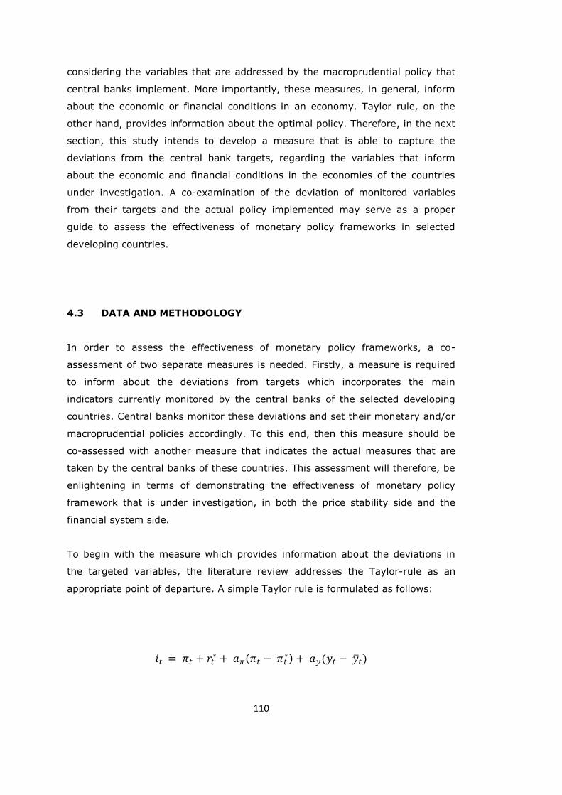
110

considering the variables that are addressed by the macroprudential policy that

central banks implement. More importantly, these measures, in general, inform

about the economic or financial conditions in an economy. Taylor rule, on the

other hand, provides information about the optimal policy. Therefore, in the next

section, this study intends to develop a measure that is able to capture the

deviations from the central bank targets, regarding the variables that inform

about the economic and financial conditions in the economies of the countries

under investigation. A co-examination of the deviation of monitored variables

from their targets and the actual policy implemented may serve as a proper

guide to assess the effectiveness of monetary policy frameworks in selected

developing countries.

4.3 DATA AND METHODOLOGY

In order to assess the effectiveness of monetary policy frameworks, a co-

assessment of two separate measures is needed. Firstly, a measure is required

to inform about the deviations from targets which incorporates the main

indicators currently monitored by the central banks of the selected developing

countries. Central banks monitor these deviations and set their monetary and/or

macroprudential policies accordingly. To this end, then this measure should be

co-assessed with another measure that indicates the actual measures that are

taken by the central banks of these countries. This assessment will therefore, be

enlightening in terms of demonstrating the effectiveness of monetary policy

framework that is under investigation, in both the price stability side and the

financial system side.

To begin with the measure which provides information about the deviations in

the targeted variables, the literature review addresses the Taylor-rule as an

appropriate point of departure. A simple Taylor rule is formulated as follows:

𝑖𝑡 = 𝜋𝑡 + 𝑟𝑡∗ + 𝑎𝜋(𝜋𝑡 − 𝜋𝑡

∗) + 𝑎𝑦(𝑦𝑡 − �̅�𝑡)

111

where 𝑖𝑡 is the short-term nominal interest rate (policy rate), 𝜋𝑡 is the realized

rate of inflation, 𝜋𝑡∗ is the desired inflation (inflation target), 𝑟𝑡

∗ is the assumed

equilibrium real interest rate, 𝑦𝑡 is the real GDP and �̅�𝑡 is the potential GDP.

Taylor (1993) proposes setting 𝑎𝜋 and 𝑎𝑦 as 0.5. Although there are different

approaches regarding the determination of these associated weights, it is certain

that the signs of these weights should be positive. The more these variables

deviate from the targets in the upward direction, the tighter the monetary policy

should become. When GDP is above its potential and inflation is higher than the

targeted level, a central bank would create a tighter policy environment whereas

when GDP is underperforming and inflation is behind the targeted level, central

bank would choose a more accommodative policy stance.

Considering Taylor’s reasoning as a useful point of departure, this study intends

to create a Policy Target Index which would incorporate the main variables that

are targeted and closely monitored by the central banks of the selected

countries. Regarding the changes occurred in the understanding of central

banking, this index is at first formed be formed for the pre-crisis period

(standard PTI) as an illustration of the reasoning and for the post-crisis period

(augmented PTI) to conduct the main analysis of this study. Then an index to

inform about the policy stance should be formed. This index should again be

differentiated for the pre- and post-crisis periods as an illustration of the

functioning of the indices and an instrument for the main analysis respectively.

The last step is to co-assess these indices.

4.3.1 Standard CBRI

The third Chapter explains the understanding of central banking practices during

the Great Moderation in detail. While constructing an instrument that intends to

evaluate central banking practices of the given era, the circumstances of the

time should be taken into account. The simplicity of the understanding of the

pre-crisis central banking practices facilitates the construction of the index to be

112

developed. Benefiting from the simplicity of the era, this section aims to form

the way of construction of the index approach which is to be used in the rest of

the study. The scaling, weighting and general reasoning that are shaped in this

section compose the basis for the analysis part in the following section.

Regarding the pre-crisis consensus on the monetary policy framework, a Policy

Target Index should then incorporate the following variables:

INF: This variable reflects the deviation of the realized inflation from the target

inflation which a central bank announces explicitly or implicitly. To avoid the

fallaciously pleasant results due to wide target ranges, all targets are set as a

point target by calculating the average of the target boundaries. The deviation

from the targeted inflation rate –either upward or downward- implies a need for

appropriate adjustments in the short-term interest rates.

GDP: The GDP variable is the remainder when the potential GDP growth

indicated by OECD (2012) is subtracted from the actual GDP growth recorded in

a country. The remainder stands for the output gap. The higher the real GDP

growth deviates away from its potential, the tighter measures are required to be

taken by the central bank.

Rather than an augmented Taylor equation, the study seeks an aggregated

index. This is because that the aim of this study is not the computation of the

exact optimal policy but to assess whether the policies implemented in selected

countries moves in conformity with the deviations of monitored indicators from

their targeted values. Therefore, to do such an assessment, another aggregated

index which indicates the overall policy stance is required. This index is the

Monetary Policy Index (MPI).

The policy toolkit of the central banks has expanded after the global financial

crisis. However, before the crisis, the characteristics of the Great Moderation

implied the control of GDP gap and inflation only through short-term interest

rates. Therefore, the standard MPI for the pre-crisis period should simply be

short-term interest-rates.

113

As indicated in the literature review, there are various ways to put the values

from different variables into the same scale. Throughout the rest of this section,

this analysis seeks ways to co-assess the deviations from targets with the

adjustments in the new policy mixes. Regarding this particular aim of this

analysis, all scaling methods can apply, however, each possessing some specific

benefits and drawbacks. The goal is to capture the method which applies the

best for this analysis.

The empirical normalization method, which scales the values according to the

min-max range functions well in terms of converting the recorded deviations

from 0 to 1. However, the background research for this study reveals that the

targets of central banks may not be adjusted so often (for example, while

inflation targets are announced each year, credit growth or current account

deficit targets are determined in line with the structure and fundamentals of the

economy and may apply for more than a year). Therefore, simply subtracting the

target from the realized value and the scaling the result (deviation from the

target) invalidates the incorporation of targets in the analysis (in the case when

targets are not adjusted frequently). The scaled values of the deviation values

give the same results when values are scaled before a normalization process.

A solution to this problem may be using absolute deviations. When absolute

deviations are applied to the analysis, the resulting values only imply the

deviations from targets, excluding an indication of the sign of the deviations. In

other words, this method allows us to only focus on the deviations regardless

whether they are upward or downward. This way, the problem with the

invalidation of the targets is fixed. However, fixing the target problem in this

manner is against the reasoning of the indices since different signs do not offset

each other. Therefore, the co-assessment with the adjustments in the policy mix

becomes unreasonable. For example, when credit growth is accelerating far

ahead of the target and real GDP growth is behind the potential, the deviations

are added regardless the signs they have. However, the expected policy

responses from a central bank would be cutting interest rates and increasing

reserve requirements. In this respect, the index for the policy mix would be

aggregated in a sense where different directions of policies offset each other

whereas the index formed for targets would stand for absolute deviations.

114

The second scaling method that is listed in the literature review is statistical

normalization (standardization). Standardized values are obtained by dividing

the difference between the given value and the mean by the standard deviation

of the data set. Similar to the case with empirical normalization, this method

also invalidates the incorporation of the targets. When a constant value

(unadjusted target in our case) is subtracted from each given value in the

dataset, the standardized values from the subtraction are equal to the directly

standardized original values. However, a simple modification fixes this problem.

The formula of standardization implies that the standardized values stand for the

distance of the original values from the mean in terms of standard deviation.

Then, if the formula incorporates the target value instead of the mean, the

obtained value is the distance from the original value from the target. Therefore,

with the mentioned modification to the standardization formula, this approach is

a simple way to measure the distance of a value from the target in terms of

standard deviations. This method, however, can no longer be defined as

standardization as known in the literature. It can rather be considered as a

transformation method to serve for the goal of this study. The formula is shown

below:

𝑇𝑟𝑎𝑛𝑠𝑓𝑜𝑟𝑚𝑒𝑑 𝑉𝑎𝑙𝑢𝑒𝑠 (𝑋𝑡,𝑖) = (𝑥𝑡,𝑖 − 𝑥𝑡,𝑖

∗ )

𝑠

Where x is the value of the variable i at time t, x* is the target value of variable i

at time t and s is the standard deviation of the x values. Since its reasoning

relies on a centralization of the deviations around the target, it is referred as the

‘Centralization Around Target’ method in the rest of the study.

After transforming the values of the selected indicators, a composite index is

formed by equal-weighting approach. There are several methods for determining

weights in the literature as indicated in this chapter earlier. However, a vast

majority of similar studies have applied equal weighting approach while

constructing their indices. Furthermore, in his study of a financial stability

115

conditions index, Van den End (2006) showed that there is a modest discrepancy

between equal weighting and weighting based on econometric validation. Illing

and Liu (2006) also put forward that equal weighting performs as well as

weighting that is predicated on economic fundamentals. Therefore the

formulations of standard and augmented PTI are given as follows:

𝑃𝑇𝐼𝑠𝑡 = 0,5 (𝑋𝑡,1) + 0,5 (𝑋𝑡,2)

where 𝑋1 is the transformed values of INF and 𝑋2 is the transformed values for

GDP.

For the construction of the standard MPI, the problem with the targets no longer

apply. Therefore, the values can be standardized with the given standardization

formula in the literature:

𝑆𝑡𝑎𝑛𝑑𝑎𝑟𝑑𝑖𝑧𝑒𝑑 𝑉𝑎𝑙𝑢𝑒𝑠 (𝑋𝑡,𝑖) = (𝑥𝑡,𝑖 − 𝑥�̅�)

𝑠

Having formed two measures that inform about the targets and the actual

monetary policy stance, the next step is the co-assessment. At this point, the

Monetary Independence (MI) index of Aizenman (2008) serves as a useful guide.

As indicated in the literature review, this is a measure which is developed to

provide information based on the extent of the relationship of two supposedly

interrelated variables. The correlation between the home and base country

interest rates are incorporated in a correlation analysis which reveals information

upon the degree of monetary independence.

In this sense, the correlation between PTI and MPI can be used to inform about

the strenght of the relationship between the aggregate deviations and the

aggregate policy stance. Following the Taylor reasoning, the closer the

movement of the actual policy to the deviations from the targets, the better the

116

central banks are responding. Rather than the effectiveness of the tools, this

relationship informs about the extent of success of the central banks in

responding the deviations in the monitored variables from their targeted values.

Therefore, a Central Bank Responsiveness Index (CBRI) should measure the

simple correlation between PTI and MPI. Since correlation analysis is invariant

to linear scaling methods, there is no need to rescale the aggregated values from

the indices.

For the formulation of the CBRI, the reasoning on the construction of the

Monetary Independence (MI) Index is followed. As stated earlier, the monetary

independence index examines the correlation between home country and base

country interest rates. The correlation that ranges between [-1,1] moves from

the lowest monetary independence to the highest. Aizenman (2008) converts the

simple correlation values that are within the range [-1,1] into the range [1,0] so

that values closer to one (zero) represents higher (lower)monetary

independence. The following formula is used for conversion:

𝑓(𝑥) = 𝐶 [1 −(𝑥−𝐴)

(𝐵−𝐴)] + 𝐷 [

(𝑥−𝐴)

(𝐵−𝐴] , where the values within the range [A,B] is

converted into the range [C,D]. In the CBRI, however, the simple correlation

values within the range [-1,1] are converted to the range within [0,1], while

lower (higher) values indicate lower (higher) responsiveness. In this respect, the

formula for the standard CBRI is given below:

𝐶𝐵𝑅𝐼𝑠𝑡 =𝑐𝑜𝑟𝑟 (𝑃𝑇𝐼𝑡,𝑖

𝑠𝑡, 𝑀𝑃𝐼𝑡+𝑚,𝑖𝑠𝑡 ) + 1

2

The data for standard CBRI is in monthly terms and covers the period from

2002M1 to 2010M10. As indicated while describing the formulation process, the

closer the values to 1, the better responding the monetary policy framework is.

For the values from the correlation analysis to be valid, the values from the two

indices should be normally distributed. For the standard MPI, we already know

that the values have a mean of zero and a standard deviation of one by

construction. However, for the PTI, a modified standardization technique is

117

applied. Therefore, the values obtained from the PTI should be checked whether

they are normally distributed. For this purpose, the bell-curves with skewness

values can be examined. A significant skewness can violate the assumptions for

the validity of the correlation analysis, and therefore the CBRI.

Figure 4.2: The Bell-Curves and Skewness Values for the Standard PTI’s of Turkey (left) and Brazil

(right)

Figure 4.2 shows the bell-curves for the standard MPI for Turkey and Brazil

respectively. The skewness values are not significant, so the data can be

assumed to be fairly symmetric. This can further be verified from Figure 4.3

which demonstrates the scatter plot diagrams obtained from the normality test.

The original values fairly coincide with the line of expected values.

Note: The black dots are plotted for z-values versus expected values and the grey ones

stand for z-values against the original sorted values.

Figure 4.3: Z-values for the Standard PTI’s of Turkey (left) and Brazil (right)

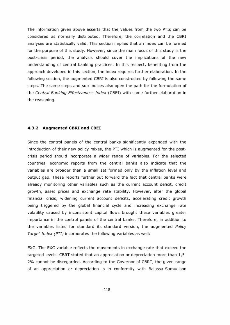
118

The information given above asserts that the values from the two PTIs can be

considered as normally distributed. Therefore, the correlation and the CBRI

analyses are statistically valid. This section implies that an index can be formed

for the purpose of this study. However, since the main focus of this study is the

post-crisis period, the analysis should cover the implications of the new

understanding of central banking practices. In this respect, benefiting from the

approach developed in this section, the index requires further elaboration. In the

following section, the augmented CBRI is also constructed by following the same

steps. The same steps and sub-indices also open the path for the formulation of

the Central Banking Effectiveness Index (CBEI) with some further elaboration in

the reasoning.

4.3.2 Augmented CBRI and CBEI

Since the control panels of the central banks significantly expanded with the

introduction of their new policy mixes, the PTI which is augmented for the post-

crisis period should incorporate a wider range of variables. For the selected

countries, economic reports from the central banks also indicate that the

variables are broader than a small set formed only by the inflation level and

output gap. These reports further put forward the fact that central banks were

already monitoring other variables such as the current account deficit, credit

growth, asset prices and exchange rate stability. However, after the global

financial crisis, widening current account deficits, accelerating credit growth

being triggered by the global financial cycle and increasing exchange rate

volatility caused by inconsistent capital flows brought these variables greater

importance in the control panels of the central banks. Therefore, in addition to

the variables listed for standard its standard version, the augmented Policy

Target Index (PTI) incorporates the following variables as well:

EXC: The EXC variable reflects the movements in exchange rate that exceed the

targeted levels. CBRT stated that an appreciation or depreciation more than 1,5-

2% cannot be disregarded. According to the Governor of CBRT, the given range

of an appreciation or depreciation is in conformity with Balassa-Samuelson

119

effects. Since there is not any rate stated by the BCB, this study considers the

same rate as the target rate for Brazil.

CRE: This variable shows the deviation of the realized credit growth rate from

the target. The credit growth data is based on the total credit provided by

domestic banks. CBRT focuses on the change in credit stock over GDP ratio –

which is approximately 55% - in determining the desired rate of credit growth.

Ranking countries according to their credit/GDP ratios, Alper et al.(2013) assert

that the 25 and 75 percent quartiles correspond to a range of 6.7-10.6 percent.

They further put forward that when Turkey’s high level of current account deficit

is also taken into account, the appropriate credit growth rate for Turkish

economy should be around 7.5% in the given range, which implies an annual

credit growth rate of 15%. In line with this reasoning, Turkish authorities

address a rate of 15% as the desired credit growth rate. On the other hand, BCB

stated the credit as growing at a sustainable pace at the level approximately

18%21. This rate is also consistent with the approach of CBRT in determining a

desirable credit growth rate. Credit/GDP ratio in Brazil was around 64%

(Worldbank, 2014) when the Turkish rate was at 55%. However, the Brazilian

current account deficit has been significantly lower than Turkeys’ with a rate

around 2,5% and 7,5% of the GDP respectively. Therefore, one would expect a

higher target for annual credit growth rate for Brazil which is in line with the

statement of the Brazilian authorities addressing an 18% target rate.

CAB: The CAB variable is the difference between the realized current account

deficit (surplus) and the targeted deficit (surplus) level. For both of the selected

countries, the current account balance for the post-crisis period record deficits.

The aim of both central banks in this front is to reduce their current account

deficit to a sustainable level. For the case of Turkey, a sustainable current

account deficit can be considered as the current account balance excluding

energy. The share of energy in the Turkish current account deficit has been

exclusively large with approximately 40% in 2011, 50% in 2012 and 30% in

2013 (CBRT). However, in Brazil, energy does not appear to be a driving force

for the current account deficit and therefore the aim of the central bank can be

21

The statements belong to Luiz Pereira, the Director of International Affairs of BCB (Bloomberg

Business, 2011) and Carlos Hamilton Araujo, Economic Policy Director of BCB (Mninews, 2012).

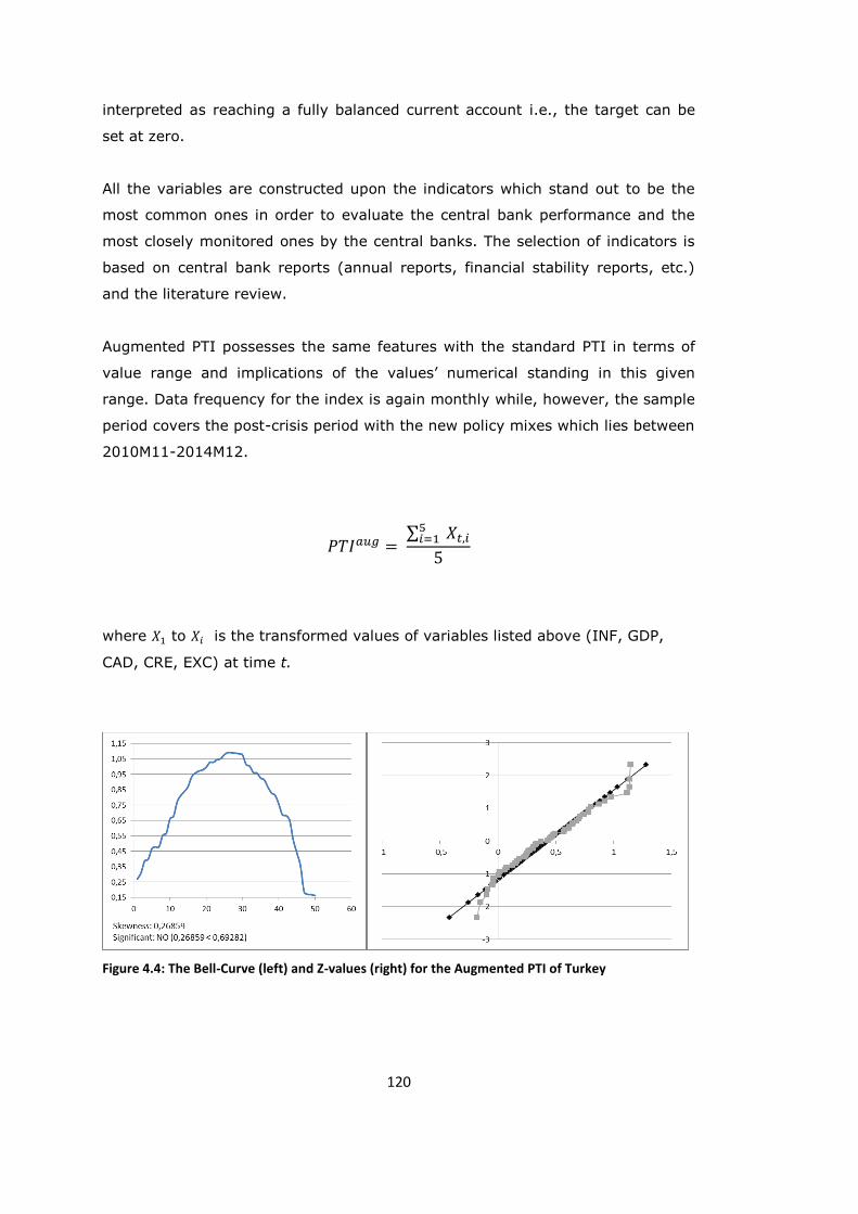
120

interpreted as reaching a fully balanced current account i.e., the target can be

set at zero.

All the variables are constructed upon the indicators which stand out to be the

most common ones in order to evaluate the central bank performance and the

most closely monitored ones by the central banks. The selection of indicators is

based on central bank reports (annual reports, financial stability reports, etc.)

and the literature review.

Augmented PTI possesses the same features with the standard PTI in terms of

value range and implications of the values’ numerical standing in this given

range. Data frequency for the index is again monthly while, however, the sample

period covers the post-crisis period with the new policy mixes which lies between

2010M11-2014M12.

𝑃𝑇𝐼𝑎𝑢𝑔 = ∑ 𝑋𝑡,𝑖

5𝑖=1

5

where 𝑋1 to 𝑋𝑖 is the transformed values of variables listed above (INF, GDP,

CAD, CRE, EXC) at time t.

Figure 4.4: The Bell-Curve (left) and Z-values (right) for the Augmented PTI of Turkey

121

Figures 4.4 and 4.5 indicate that the values from augmented PTI’s can also be

considered as normally distributed. Bell-curves for both Brazilian and Turkish PTI

imply skewness values that are not significant and original sorted values coincide

with the expected values.

Figure 4.5: The Bell-Curve (left) and Z-values (right) for the Augmented PTI of Brazil

While the control panels of the central banks have expanded, their toolkits to

control these variables have enhanced too. As with the standard analysis,

another aggregated index which indicates the overall policy stance is required for

the augmented analysis. The standard MPI for the pre-crisis period is simply

composed of short-term interest-rates. In line with the enhanced toolkits of the

central banks after the global financial crisis, the augmented MPI should

incorporate the tools in the new policy mixes of two selected countries as

summarized in Table 4.1 below.

For both countries, the policy rate and three macroprudential policy tools are

included. Values from each tool are statistically normalized so that they have a

mean of zero and a standard deviation of one. After the standardization process,

each indicator is associated with equal weights. Since policy rate covers a larger

part of a monetary policy framework and macroprudential policies are adjusted

less frequently, the study also attempts to associate policy rates with a higher

weight whereas macroprudential policies are assigned by a lower weight.

122

Table 4.1: Monetary Policy Tools included in the Monetary Policy Index

*Weighted average23

**The width of the corridor

However, as in the other studies in the literature summarized before, the two

methods reveal very similar results. Therefore, this analysis moves on with the

equal weighting approach. The final formulation of the MPI is given below:

𝑀𝑃𝐼𝑎𝑢𝑔 = 0,25 𝑃 + 0,25 𝑀𝐴𝑃𝑃1 + 0,25 𝑀𝐴𝑃𝑃2 + 0,25 𝑀𝐴𝑃𝑃3

Where P stands for short-term interest rates set by the central bank (policy rate)

and 𝑀𝐴𝑃𝑃 represents the three selected macroprudential policies being

implemented in a certain country (see Table 4.1). Having constructed the

augmented versions of PTI and MPI, the augmented CBRI is formed as the

standard version.

A CBRI based on Taylor-rule reasoning indicates about the success of central

banks in responding the deviations in the mainly monitored variables. However,

the primary aim of this study is to inform about the effectiveness of the new

policy mixes. This method allows us to conduct an effectiveness analysis too.

22

Although ROM is stated as an important tool in the Turkish policy mix by CBRT, it is not included

in the augmented MPI. Since ROM is a mechanism that its utilization is in voluntarily terms, the

adjustments of the CBRT do not necessarily imply that these given changes are in effect. Therefore,

rather than the adjustments of the CBRT, ROM functions depending on the utilization of banks. In

this respect, ROM is not included in order to keep the analysis as simple as possible at this point. The

case with ROM is discussed in the robustness checks section later.

23

While computing the weighted average, the weights are set as the maturities (in terms of days) that

the IOF ratios are designed to address. This method allows the overall values to both reflect the tax

ratios and the maturities.

Country Brazil Turkey22

Important Tools in the Policy

Toolkit

Selic Rate

IOF*

RR*

FX RR

Repo Rate

Interest Rate Corridor**

RR*

FX RR*

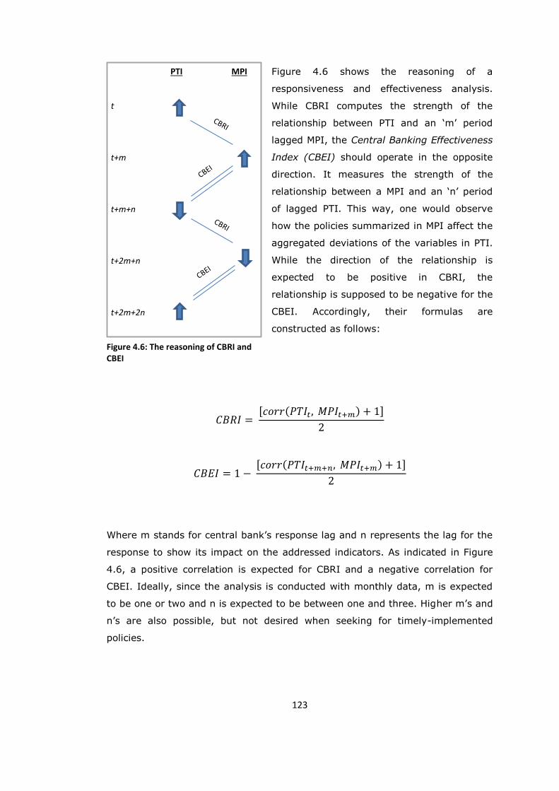
123

PTI MPI

t

t+m

t+m+n

t+2m+n

t+2m+2n

Figure 4.6: The reasoning of CBRI and CBEI

Figure 4.6 shows the reasoning of a

responsiveness and effectiveness analysis.

While CBRI computes the strength of the

relationship between PTI and an ‘m’ period

lagged MPI, the Central Banking Effectiveness

Index (CBEI) should operate in the opposite

direction. It measures the strength of the

relationship between a MPI and an ‘n’ period

of lagged PTI. This way, one would observe

how the policies summarized in MPI affect the

aggregated deviations of the variables in PTI.

While the direction of the relationship is

expected to be positive in CBRI, the

relationship is supposed to be negative for the

CBEI. Accordingly, their formulas are

constructed as follows:

𝐶𝐵𝑅𝐼 = [𝑐𝑜𝑟𝑟(𝑃𝑇𝐼𝑡, 𝑀𝑃𝐼𝑡+𝑚) + 1]

2

𝐶𝐵𝐸𝐼 = 1 − [𝑐𝑜𝑟𝑟(𝑃𝑇𝐼𝑡+𝑚+𝑛, 𝑀𝑃𝐼𝑡+𝑚) + 1]

2

Where m stands for central bank’s response lag and n represents the lag for the

response to show its impact on the addressed indicators. As indicated in Figure

4.6, a positive correlation is expected for CBRI and a negative correlation for

CBEI. Ideally, since the analysis is conducted with monthly data, m is expected

to be one or two and n is expected to be between one and three. Higher m’s and

n’s are also possible, but not desired when seeking for timely-implemented

policies.

124

The data for CBRI and CBEI is available for the post-crisis period starting from

the date of adoption of new policy mixes, 2010M11-2014M12. The data sources

are: IMF BOPS Database, UNStats, BIS Exchange Rate Database and the

websites of BCB and CBRT for monthly series included in the PTI; policy reports

and related speechs from central bank governors for targets settings; and again

websites of BCB and CBRT for the time-series data upon monetary and

macroprudential policies included in MPI.

There are several benefits of this approach. First of all, monetary policy cannot

be considered to be composed of simply policy rates anymore. The lessons from

the global financial crisis brought the introduction or bolstering of the

macroprudential policy. The policy responses of central banks should be

investigated at the aggregate level, covering both short-term policy interest

rates and macroprudential tools. In this respect, MPI is the first measure in the

literature with the intention of informing about the overall policy stance, covering

both monetary and macroprudential tools.

Secondly, central banks do no longer aim only to promote price stability and

control output gap. With the introduction of the financial stability into central

bank objectives, financial system indicators, which were partially monitored

before the global financial crisis, have also taken part in the control panels of the

central banks. The control panels of the developing countries are now broader to

include current account deficit, credit growth and exchange rate, especially for

the selected countries. Therefore, the PTI stands out to be an index broad

enough to cover almost all of the main indicators that are closely monitored by

the central banks. In addition to the five selected indicators, more indicators can

be included in the analysis when desired. In this vein, CBRI and CBEI are the

first indices in the literature that are capable to assess the relationship between

central bank reactions and the movements in an economy.

Thirdly, CBEI covers all interactions that occur within the sub-indices. When, for

example, monitored indicators deviate from targets in the opposite directions, it

is expected that this would be reflected as in an aggregate sign and size in the

policy target index. In other words, when GDP is far behind the potential rate

and credit growth is accelerating with a significant positive deviation from the

125

target, policy rates and reserve requirements are implemented in the opposite

ways too. As a response to the deviations from the targets, central banks would

supposedly cut interest rates and increase reserve requirements. The indicators

that move in the opposite directions are represented in the indices with the final

sign and magnitude of all indicators after the aggregation process. This enables

an analysis that does not only measure the effectiveness of certain policies on

certain indicators but also assesses the overall effectiveness which also takes

interactions into account. Therefore, with this reasoning, a monetary policy

framework which benefits from interactions in a correct way, are associated with

a higher effectiveness by the CBEI.

Lastly, this method intends to overcome the simultaneity problem arisen from

the correlation analysis. Correlation analyses typically do not inform about

causality. They rather observe the simultaneous movements among the

indicators. By incorporating lagged versions of PTI and MPI respectively, the

method attempts to overcome the simultaneity problem in the results obtained

from the CBRI and CBEI. This way, CBRI directly informs about the extent that

central banks can respond to the deviations of variables in their control panel

from their targets or trends. The ability of the central bank measures to capture

the deviations from their targets increases the responsiveness. In this case, the

values from the CBRI should approach through one. The same case applies for

the effectiveness analysis with CBEI.

There are also some limitations of this approach. Central banks may tend to

operate their policies in an asymmetric manner. A central bank, for example,

may intervene in the foreign exchange market in the case of a domestic currency

depreciation whereas it may tolerate a domestic currency appreciation (for the

Turkish, S.African, Brazilian and Mexican cases: see Benlialper and Comert,

2013;Heintz and Ndikumana, 2010; Barbosa-Filho, 2006 and Galindo and Ros,

2008, respectively). Implementing such type of a policy, central banks use

exchange rates as a tool to achieve their inflation targets rather than a

monitored indicator. The CBRI simply considers such an asymmetric behavior

towards any of the listed indicators as a lack of responsiveness and the values

will diverge from 1. The lack of responsiveness should also decrease the values

for CBEI.

126

Another shortcoming is that since MPI does not contain all central banking

practices such as open market operations, the measures taken by other

regulatory bodies (such as BRSA in Turkey) and the rest of the macroprudential

tools that are being implemented, the indices are not expected to be very close

to 1. Nevertheless, the measures that are included are the most frequently used

ones among the toolkits and stand out to be the ones that central banks attach

the most importance to. Therefore, even though the indices are not expected to

be very close to 1, the results still indicate crucial information upon the

effectiveness of pre- and post-crisis monetary policy frameworks. Other

drawbacks still exist, but tried to have been minimized. These are given

throughout the analysis and conclusion when relevant.

4.4 RESULTS

This approach allows us to make a detailed assessment. The results obtained

from the indices are interpreted in four main aspects:

Simultaneous assessment of responsiveness and effectiveness: The two separate

measures on the same data set allow us to easily investigate the standanding of

a central bank in terms of effectiveness. When responsiveness is high, but

effectiveness is not satisfactory, there might be an undesired interaction among

the policies which limits the effectiveness of the policy mix. Furthermore,

assessing effectiveness solely may be misleading. Other conditions may drive the

desired results rather than the policies of the central bank. A central bank can

take advantage of other conditions to reach their desired results. Co-assessment

with the resposiveness is more informative in that sense.

Examination of the resistence of policies against global conditions : Data is

divided into sub-periods. Two additional sub-sample periods are added to the

entire sample period: 2010M11-2013M5, 2013M5-2014M12 where 2010M11

stands for the time of adoption of the new policy mixes and 2013M5 represents

the time when US Fed announced the possible tapering of its QE policies in the

127

following months. Chapter 3 explains in detail how US tapering policy caused

capital outflows and depreciation pressures for developing countries. Regarding

the extent of the global shock, this date appears to be the first serious test for

the post-crisis policy mixes of developing countries.

Note: The horizontal axis represent the lagged time. Then t=49 above and t=47 below refers to

2014M12.

Figure 4.7: Co-movement of the sub-indices for responsiveness (above) and effectiveness (below)

analysis

Cross-country comparison: The central banks of both Brazil and Turkey

announced their adoption of new policy mixes in late 2010. Moreover, as

indicated in the previous Chapter in detail, their economies share similar risks.

Therefore, a cross-country comparison should reveal important implications upon

a successful policy mix. Moreover, the sub-sample periods mentioned in the

points above are also subject to a cross-country comparison, since the inequally

distributed length of data among periods may be misleading.

128

Figure 4.7 shows the co-movement of the PTI and MPI for both Turkish and

Brazilian cases. In the figures above where m=1, the MPI follows PTI with a one

month lag whereas the figures below where n=2, the PTI follows MPI with a

three months lag (m+n=3). From the first relationship, a positively co-

movement is observed. This is consistent with the reasoning of this study. The

second relationship is also in conformity with the expectations, since a fairly

negative co-movement is reflected.

Table 4.2: CBRI and CBEI results (monthly)24

Table 4.2 lists the results from the CBRI and CBEI. To begin with the

responsiveness analysis, BCB seems to have been more successful than CBRT.

Both of the central banks have better responsiveness values before the Fed

tapering talk. As stated before, the MPI for both countries do not include all the

measures implemented by their central banks. Therefore, these values only

represent the responds of the central banks for the included policy tools. In this

sense, the responsiveness values for the pre-tapering talk period are in

conformity with the expectations of this study.

The analysis in the responsiveness front let us assume that a timely-response

should take one month for a central bank after a non-negligible deviation takes

place. Taking this into account, it is reasonable to expect that the impacts of the

policies should become evident in the next two, three months or so on.

Nevertheless, the values with any lag provide results in a similar direction, i.e.,

24

Correlation values are given in Table B.1, Appendix B.

m=1 m=2 m=3 m=1 m=2 m=3

2010M11-2014M12 0,587303 0,617591 0,594821 0,653286 0,704824 0,755416

2010M11-2013M5 0,727787 0,769589 0,746682 0,600929 0,701744 0,791247

2013M5-2014M12 0,248748 0,307342 0,301206 0,457543 0,21883 0,249717

(assuming m is 1) n=1 n=2 n=3 n=4 n=1 n=2 n=3 n=4

2010M11-2014M12 0,494885 0,530978 0,527797 0,494626 0,516077 0,56027 0,599564 0,627783

2010M11-2013M5 0,511761 0,591321 0,611134 0,5612 0,647981 0,706616 0,772299 0,81704

2013M5-2014M12 0,464739 0,370626 0,400369 0,422383 0,345477 0,520959 0,455979 0,519498

CBRI

CBEI CBEI

CBRI

TURKEY BRAZIL

129

values computed with all lags decrease after the Fed tapering talk. This is

consistent with the findings in the previous Chapter. In the setting of lags, any

lag can be utilized regarding the circumstances of the specific economy and

policy mix, as long as the main reasoning (1≤m<m+n) holds.

For Turkey, both the response and effectiveness lags appear to be shorter. This

is consistent with the design of the Turkish policy mix. CBRT presents the

interest rate corridor as a tool which allows timely-implemented adjustments.

On the other hand, the examination of the Brazilian policy mix carried out in

Chapter 3 shows that the included tools are not easily adjustable or adjusted

frequently by BCB. The IOF measures, as includes the imposition of different

types of financial transactions taxes, are not easily adjustable. BCB imposes or

eliminates these measures rather than adjusting them at different rates.

Moreover, the FX RRs which can be easily adjusted as in the case of Turkey, are

also imposed at a high rate and then eliminated without being adjusted by BCB

within this time frame. Therefore, when these specific characteristics of the

policy mixes are also taken into account, it is reasonable to reach the conclusion

from the indices that CBRT obtains its desired results in a faster pace.

While the Turkish policy mix overperforms with respect to the Brazilian mix in

terms of timing, the effectiveness front reveal opposite findings. The values from

the CBEI demonstrate that the policies of BCB have been remarkably more

effective than those of CBRT. Especially in the last sub-sample period where both

effectiveness values are deteriorated significantly, BCB managed to maintain its

control over the targeted variables. For CBRT, the effectiveness values are

already unlikely to be meaningful since the responsiveness is almost vanished.

For an interaction analysis, the results do not directly assert any findings.

However, some implications can be reached. In the Brazilian values from late

2010 to mid-2013, the CBEI value exceeds the CBRI value. However, Turkish

CBEI falls way behind the CBRI for the same period. Although further

investigation is needed, this may be an indicator of an undesired interaction

within the Turkish policy mix.

130

4.5 ROBUSTNESS CHECKS

To check whether the results obtained from the CBRI and CBEI are accurate and

consistent with the facts revealed in the previous chapter, some further

investigation is required. First step is to conduct the same monthly analysis with

absolute deviations instead of total deviations. Secondly, the analysis is focused

on the Turkish case, particularly on the ROM. Furthermore, the relationship

between central bank effectiveness and global conditions is investigated. Finally,

the analysis further incorporates the financial soundness indicators into the PTI.

The first step is to conduct the same analysis with absolute deviations i.e.,

disregarding the signs of the deviations. The analyses until this point are

conducted with the assumption that central banks adjust their policies by taking

the aggregate sign and size of the deviations into account. This step is a useful

way to check the validity of this assumption. Since the sign of the deviations are

neglected, the original standardization formula is used for the calculation of PTI.

The results are given in Table B.2 in the B section of the Appendices. The

findings reveal significantly inconsistent results by giving same signs of

correlation values for both CBRI and CBEI. Therefore, it can be concluded that

absolute deviations are not taken into account by central banks and the main

assumption of this study is valid.

The second step is to elaborate on the Turkish case with ROM. While conducting

the analyses throughout this chapter, the Turkish policy mix has been simplified

by excluding ROM from the MPI. The reason to take the case of ROM separately

is because of the fact that its way of implementation and functioning may cause

some problems. ROM has been in effect since late 2011. However, its

introduction came in multiple steps and it became fully in effect after mid-2012.

Moreover, as explained in detail in Chapter 3, ROM’s utilization by banks is based

on voluntariness. CBRT sets the ROC (Reserve Option Coefficient) in response to

the developments in the economy whereas banks make their own decisions on

the utilization of the ROM accounts. The findings in Chapter 3 reveal that mainly

after the Fed tapering talk, banks have not been utilized the ROM facility in line

131

with the CBRT’s expectations. Therefore, the results with ROM are not expected

to have a positive impact on our indices after the tapering talk.

PTI MPI

t

t+m

t+m+n

Figure 4.8: The Reasoning of the Main Indices

To include ROM in the MPI, its functioning

should be consistent with the reasoning of

the CBRT and CBEI. When there is a large

surge of capital inflows and domestic

currency is appreciating (Figure 4.8, time t),

banks are expected to use the ROM facility

by holding extra surges in ROM accounts.

Central bank decides on the size of reserves

that can be held in FX by adjusting ROC

(reserve option coefficient).

This way, the appreciation pressures on the domestic exchange rate is supposed

to be reduced (Figure 4.8, time t+m+n). Hence, the functioning of ROM is

consistent with the reasoning of CBRI and CBEI. As already mentioned, its

introduction came in multiple steps. Therefore, since the results from CBRI are

not likely to yield any meaningful findings, the analysis is conducted solely with

the CBEI.

Table 4.3: CBEI results for Turkey computed with and without ROM2526

25

Correlation values are given in Table B.3, Appendix B.

26

It is already stated in earlier that all lag settings lead similar conclusions. For simplicity, the values

represent the lag setting of three (m+n=3) for CBEI analysis after this point, unless otherwise stated.

2011M10-2013M5

WITHOUT ROM

WITH ROM

2013M5-2014M12

0,412781754 0,37062551

0,487399224 0,368791757

132

The findings from CBEI that is computed with and without ROM are listed in

Table 4.3. The findings are consistent with the expected results. Before the Fed

tapering talk, when banks used the ROM facility as desired by the CBRT, the

inclusion of ROM seems to have led an increase in the effectiveness. However,

after May 2013, effectiveness decrease since banks used ROM in contrast to its

aim of design. These findings support the conclusion in Chapter 3 that the

benefits of ROM may have been weakened by its joint use with the interest rate

corridor. Until mid-2013, when capital inflows persisted, the utilization of ROM

facility helped the control of exchange rate volatility by reducing appreciation

pressures. On the other hand, after mid-2013, when capital outflows took place,

CBRT increased the upper bound of the interest rate corridor and thus made the

utilization of ROM facility more profitable for banks. Although banks were

expected to withdraw their FX reserves in ROM and decrease depreciation

pressures on TL, this undesired behavior caused further depreciation of TL.

Another implication from Chapter 3 is that CBRT mainly lost its control on the

targeted indicators after mid-2012. The Chapter also asserts that although the

loss of control date back to mid-2012, the observable disruption on the main

monitored indicators took place with the Fed tapering talk. To test whether this

conclusion is consistent with the index approach, the data should be divided into

further sub-sample periods.

Table 4.4: CBEI Values for Three Sub-Sample Periods27

Figure 4.9 and Table 4.4 divide the data into three sub-sample periods. First

period is from the introduction of the new policy mixes to mid-2012, where the

Turkish policy mix is deemed to be most effective. Results from Table 4.4 verify

that the first sub-sample period was the most effective period of the Turkish

policy mix. Although the Brazilian value exceeds the Turkish CBEI result, it

27

Correlation values are given in Table B.4, Appendix B.

2010M11-2012M6 2012M6-2013M5 2013M5-2014M12

Turkey

Brazil

0,37062551

0,785975761 0,930415143 0,520958981

0,758108054 0,700446607

133

should be noted that the BRSA measures which were very effective in this

period28 is excluded from this analysis.

Figure 4.9: The Strength of the Relationship Between the Turkish (left) and Brazilian (right) PTI’s

with VIX

Furthermore, the co-analysis of Table 4.4 and Figure 4.9 also put forward the

fact that this is a period where the deviations from Turkish targets were almost

independent from global factors. This can be clearly seen from Figure 4.9 which

demonstrates the strength of the relationship between PTI and VIX. In Brazil, on

the other hand, the deviations were extremely dependent to the global factors in

this period, which addresses the fact that the effectiveness of the BCB may have

owed to global conditions to some extent.

For the second sub-sample period from mid-2012 to mid-2013, CBEI values

assert that this period may have been the breaking point for the success of the

two central banks. As indicated before, Turkish CBEI value is not deteriorated

significantly. However, Figure 4.9 reflects interesting results for this period. The

strength of the relationship between the Turkish PTI and VIX increased

significantly whereas in Brazil, the relationship seems to have almost vanished.

28

See Chapter 3.

Correlation Values for PTI (Absolute Deviations) and VIX

(Denklemi buraya yazın.

134

According to the facts that are put forward in Chapter 3, this opposite movement

of the correlation in Turkey and Brazil may mostly be due to their levels of short-

term external debt and the interrelated capital flow management strategies that

they have been following.

Taking this implication into account, one can conclude that the fairly good

effectiveness value of CBRT is mostly supported by the global factors. The capital

inflows persisted in the sub-sample period under investigation, which led the

effectiveness value to be fallaciously high. On the other hand, it would be fairly

reasonable to put forward that BCB showed a remarkable success in this period,

since PTI was not driven by the external factors.

Figure 4.9 draws an even more interesting picture for the last sub-sample period

which is from mid-2013 to the end of 2014. For this period, looking back to the

main analysis of this study with two sub-sample periods, we know that both

central banks failed to be effective to some degree. This lack of effectiveness is

also clearly seen in the current analysis. Figure enriches the analysis with more

informative results. While the sign of correlation between the Turkish PTI and

VIX was positive in the second sub-sample period, the sign becomes negative in

the third sub-sample period. The change in the sign of the correlation has

important implications when interpreting the effectiveness results for Turkey.

After 2013, the decline in the global uncertainty implied the end of the easy

money era, unlike the previous period. Figure 4.10 demonstrates the evolution

of VIX. In the second sub-sample period, a fall (rise) in the global uncertainty

would often imply more capital inflows (outflows) for a developing country. In

Turkey, where the policy mix is designed to be more market-friendly and have

less controls on the financial flows, the surges are more likely to cause

deviations. However, this positive relationship may not hold in the last sub-

sample period. After mid-2013, a decline in the global uncertainty does not

necessarily lead capital inflow surges.

Therefore, while the global conditions helped the CBRT to reach its pre-

determined targets from mid-2012 to mid-2013, the correlation having an

opposite direction in the third sub-sample period made the task of CBRT harder.

135

As a result, the effectiveness value of CBRT falls remarkably and to a larger

extent when compared with the Brazilian example.

Source: Chicago Board Options Exchange

Note: The dates associated with capital inflows and outflows can be

found in Figure 3.3 in Chapter 3

Figure 4.10: Global Uncertainty in the Sub-Sample Periods Under Investigation

In Brazil, where the correlation of PTI and VIX is still at a very low level, the

effectiveness has been reduced. Even though the credit growth level have fallen

significantly below the target and Brazilian Real have been following a sharp

depreciation trend, CBEI value decreases in a smaller extent. These findings are

likely to assert that Brazilian authorities have formed a much resistant

macroprudential framework with respect to their Turkish peers, verifying the

results from Chapter 3. Brazil had already implemented aggressive capital

control measures until 2012 so that the easy money of the date was not allowed

to enter in the country at the levels received by the Turkish economy. Therefore,

the end of the easy money era did not hit the effectiveness of BCB as

experienced by CBRT.

As the last step of robustness checks, financial soundness indicators are included

in the analysis. Since the data obtained from the IMF Financial Soundness

Indicators Database are in quarterly frequency, the analysis has to be conducted

with the quarterly version of the indices. A background analysis with quarterly

136

data reveals that the Brazilian case is more appropriate for such analysis29.

Therefore, the analysis to observe the impacts of the inclusion of financial

soundness indicators should be carried out on the Brazilian case.

There are a wide set of financial soundness indicators listed in the IMF database.

Here, a sub-set is incorporated for the construction of a Financial Soundness

Index (FSI). The FSI is based on six different financial soundness indicators

namely: i) non-performing loans to gross total loans; ii) liquid assets to short-

term liabilities; iii) net open position in foreign-exchange to capital; iv) foreign

currency denominated liabilities to total liabilities; v) household debt to GDP and

lastly; vi) residential real estate loans to total loans. These indicators allow us to

track the asset quality, covering currency and maturity mismatch problems.

Moreover, deposit takers’ exposure to exchange rate related risks and the

household indebtedness are also covered. A significant deviation in these

variables may lead potential vulnerabilities in the financial system.

Since central banks do not announce any pre-determined targets for the

indicators mentioned above, the deviations are computed with respect to the

trend. Rather than a linear trend function, a logarithmic trend line is utilized to

obtain the deviations, due to computational reasons. The remaining values are

then converted into the same scale by simple standardization and aggregated by

taking their arithmetic mean to form the FSI. The FSI is then included in the PTI

as a sixth variable.

Results are given in C section of the Appendices part. The findings reveal that

the Brazilian policy mix have been effective in controlling financial soundness.

The effectiveness values from CBEI rise for each period with the introduction of

FSI into the PTI. The most remarkable rise takes place in the last sub-sample

period, asserting that even though the Brazilian authorities have not been able

to handle the post-tapering talk period as successfully as before, they managed

to control the financial soundness effectively. This is again likely to be due to the

effectiveness of BCB curbing the short-term external debt in the previous period

29

The Turkish quarterly data does not yield accurate results. This inaccuracy may arise from shorter

response lags of the Turkish mix or simply the lack of sufficient sample periods due to quarterly

frequency.

137

and therefore having managed to establish sound macroprudential

fundamentals.

4.6 CONCLUSION

The analysis conducted in this Chapter fairly match with the implications in the

earlier Chapters. Providing a numerical value upon the responsiveness and

effectiveness, the findings are more precise and complement the intuitions

throughout the study. Moreover, the method developed in this Chapter also

leads a more detailed assessment by providing further implications on the extent

of timely-implementation, commitment to targets and dependence on external

conditions.

The CBEI show that the Brazilian policy mix has been more effective than the

one developed by CBRT. Evidence asserts that this is most likely to be a result of

the weakening of the dependence on external factors in Brazil. The earlier

analysis on the policy mix implies that this success is due to the use of capital

flow management tools that were previously known as capital controls. Yet, the

effectiveness values do not exceed the Turkish values in a remarkable manner.

Turning again back to the previous analysis in Chapter 3, it is possible to

conclude that the effectiveness of the Brazilian policy mix may have been

constrained by the distortionary effects of the capital controls. However, the

comparison with the Turkish case asserts that the benefits of the capital controls

have been more significant than their drawbacks. Even though the volatility of

the exchange rate could also have not been managed, Brazilian effectiveness

value is still higher than the Turkish.

The results obtained from the indices also assert that the Turkish policy mix

have been implemented more timely that the Brazilian mix. This is in line with

the intentions of the design of the Turkish policy mix. In this respect, CBRT have

achieved one of its goals. The interest rate corridor and ROM are tools that are

easy to respond to the changes in the monitored indicators in a timely-manner.

Moreover, evidence from Chapter 3 shows that the Turkish credit growth has not

138

been subject to any distortionary effects. Instead, the acceleration was slowed-

down by the policies of CBRT that addressed the domestic credit cycle. However,

as stated above, the effectiveness values for the Turkish policy mix are found to

be lower than the Brazilian case. This asserts that although the Turkish mix

stands to be successful in the ways given earlier, the drawbacks of the market-

friendly design exceed its benefits. The analysis which incorporates the VIX imply

that the success of the Turkish policy mix have become highly dependent on

external factors after mid-2012. The relationship was in positive terms from mid-

2012 to mid-2013, i.e. regarding the high effectiveness value for this sub-period,

Turkish policy mix may have been benefiting from the global conditions until Fed

tapering talk in May, 2013. After the given date, the relationship appears to be

negative, the exact same time that the effectiveness of the policy mix weakens.

Furthermore, the weakening of the effectiveness of ROM after Fed tapering talk

is verified by the CBEI where MPI also incorporates the ROM. Chapter 3 asserts

that this weakening may have arisen from the undesired interactions among the

Turkish policy toolkit.

This Chapter also verifies the argument presented throughout the study that the

design of the policy mix requires more attention than the selection of certain

tools. With this method, the interactions occurring in the policy mix are taken

into account. This is the first methodology that is developed in the literature with

such concern.

Although this method has important benefits, the indices can be developed

further by elaborating on certain issues so that the functioning and explanation

power of the indices can be enhanced. These issues are composed of several

points.

Firstly, some tools are excluded from PTI and MPI for computational reasons and

simplicity. PTI does not incorporate all the indicators monitored by central banks.

The indicators are selected carefully from a large set so that they would not

eliminate the significance of each other within the index. To avoid any undesired

invalidation within the index, the indicators do not reflect the complete set of

monitored indicators by central banks. For example, even though the ratio of

short-term over total external debt is an important indicator to monitor, the

139

background analysis shows that its inclusion weakens the explanation power of

the indices. This may most likely be a result of the interaction of the given ratio

with another indicator within the index, particularly the current account deficit

and/or the exchange rate. Furthermore, any indicator related to reserves is also

not included regarding the close relationship of such indicator with exchange

rates and current account balance. Moreover, FX interventions are also not

included in the PTI. Such tools can be converted into a dummy structured

variable to be incorporated by the index. In addition, the literature review earlier

underlines the importance of the banking sector indicators for assessing the case

of developing countries. In this respect, an FSI constructed with monthly data

may be included for the coverage of the entire financial system.

Secondly, although this study checks for basic statistical properties, further

investigation may be needed. This study only checks for normal distribution of

the values obtained from the `centralization around target` method.

Furthermore, the indices developed in this study may suffer from the criticisms

of Eika et al. (1996) regarding the Monetary Conditions Indices. Although their

first criticism that ‘indices may be inappropriate when policymakers have more

than one objective’ is overcome in this study, their other criticisms may remain

valid. These consist of the need for detailed examinations such as co-integration

and omitted variables. Moreover, since the formation of the CBRI and CBEI is

based on the reasoning of the Taylor rule and the construction of the Aizenman’s

Monetary Independence Index, criticisms on these studies may apply to the

indices formulated in this study as well.

Thirdly, attempts to formulate the indices show that equal-weighting method

provides more or less similar results to those when weights are differentiated for

variables. However, weights can be calculated by different empirical methods

that are used in the literature. These are simulations with macroeconomic

models, VAR models, reduced-form demand equations or the principal

components approach. This way of weight setting may be more reasonable since

central banks tend to put more emphasis on certain tools and/or may monitor

some indicators. Moreover, the associated weights can vary over time. In this

case, the Kalman filter method which is used by Montagnoli and Napolitano

(2004) in determining the associated weights for their FCI can be applied. Other

140

methods in the literature may also apply as long as they are appropriate to

reflect the choices of central banks changing through time.

As a first attempt, this Chapter contributes to the existing literature by opening a

way for the assessment of the post-crisis policy mixes. The methodology allows

a comprehensive evaluation over the central bank performance. With further

elaboration on the given issues above, the functioning of the indices can be

enhanced and they can be developed to provide more information.

141

CHAPTER 5

CONCLUDING REMARKS

Throughout this study, the design and effectiveness of the new policy mixes in

the post-crisis era of central banking are assessed. The first Chapter emphasizes

the emergence of the need for customized policy mixes in developing countries.

The last two Chapters attempt to evaluate the cases of some selected countries.

While Chapter 3 forms a basis for Chapter 4, the event analysis in the former

and the index analysis in the latter complement each other in reaching some

important conclusions upon the effectiveness of the new policy mixes.

Firstly, a policy mix should be comprehensive. Neglecting one important step of

the risk cycle may lead worsening in other steps. In the case of S.Korea the lack

of efforts to control the rise of the current account surplus led an over-

appreciating domestic currency. In turn, real GDP growth rate and inflation fell to

undesired levels. Similar chains of events are also observable in the cases of

other countries under investigation. The lack of efforts to fix the maturity

composition of capital flows into Turkey led significant worsening of the maturity

mismatch related risks which may lead abrupt results in a case of volatility in

any step of the risk cycle. Secondly, the comparison between the use of capital

controls and market-friendly policies reveals some implications. Both the event

and the index analyses assert that the capital flow management tools, which

were previously known as capital controls are more successful in controlling the

maturity composition of capital inflows. In this sense, they are more effective in

reducing the vulnerabilities of an economy against global conditions. However,

there are also some findings that these tools may lead distortionary effects over

credit and real GDP growth. Thirdly, the assessment put forward that efficacy

does not necessarily guarantee effectiveness. Even though the Turkish policy

toolkit benefits from efficacy, Brazilian policy mix appears to be more effective

142

than the Turkish policy toolkit. However, when the S.Korean policy mix is

assessed in the financial stability front, it is possible to state that S.Korean

policymakers achieved to develop a toolkit that is both efficient and effective.

Fourthly, side effects of the included tools should be investigated carefully and

complemented with additional tools where necessary. The Brazilian case related

to the side effects of IOF over exchange rate form the basis for this conclusion.

The side effects of IOF measures over the exchange rate could have been

compensated with more active use of FX RRs or the introduction of Turkish ROM

tool. The last but not the least, although complementary tools should be used

where necessary, the interaction between tools should be carefully assessed so

that no undesired interactions to take place. The implication from Chapter 3 is

supported by the findings of Chapter 4, in the sense that the effectiveness of

ROM is constrained by its interaction with another cornerstone of the Turkish

policy mix, the interest rate corridor.

The findings explained above are crucial since they attempt to form a basis for

the possible adjustments to the policy mixes of the selected developing

countries. They also intend to form some possible guidelines for policymakers of

countries where the design of the new policy mixes is yet in progress. With

further elaboration on these issues, toolkits that are optimized to enhance

macroeconomic and financial stability may become more likely to be promoted.

Nonetheless, the main contribution of this study to the existing literature is the

new approach that is developed to assess the central bank responsiveness and

effectiveness in the post-crisis era. The two indices –Central Bank

Responsiveness Index and Central Bank Effectiveness Index – are constructed

upon a wide review on the indices that are developed in the literature until this

date. Yet, they are based on a simple reasoning. The findings from the indices

imply similar or complementary findings to those from the event analysis.

Moreover, they also provide some additional information where event analysis

falls short to compute such as: the extent of timely-implementation of the

policies or commitment of central bank to its pre-determined targets.

Nevertheless, the most important feature stands out to be providing numerical

values upon the effectiveness of overall policy frameworks. This feature

facilitates to conduct a comprehensive assessment and also a cross-country or

cross-period comparison.

143

Since this is a very first attempt to conduct such an analysis, the methodology

can be subject to some adjustments in order to enhance the explanation power

of the indices. First, the sub-indices may suffer from excluded variables. PTI can

incorporate some additional indicators that central banks monitor. A more

sophisticated MPI can also be developed by taking the excluded tools into

account. Further elaboration on the sub-indices may help the main indices to

better function and provide more precise results. Moreover, the determination of

targets in this study is based on non-official statements in some cases.

Availability of official central bank statements, policy reports or speeches from

governors may optimize the target setting and lead healthier information to be

provided by the indices upon the effectiveness of central banks. Lastly, a more

detailed assessment on the statistical properties of the indices and further

considerations on the setting of the weights for the variables that compose the

sub-indices may be possible.

Taking the given possible adjustments to the indices into account, this first

attempt opens a way for prospective studies that would benefit from the given

approach. First, the simplicity of the approach makes them possible to be

adjusted for any country. The indicators in PTI and the tools in MPI can be

selected in accordance with the circumstances in a country. Second, the indices

can be simplified, enhanced or modified in any sense as long as the alterations

are in line with the reasoning behind the construction of the indices. The indices

are incorporated to enlighten the post-crisis era of central banking in this study.

However, they can also be adjusted for studies that would seek historical

findings. In addition, they can also be enhanced or modified for any

developments that would occur in central banking practices in the future. Third,

in empirical studies where the time span of the data is sufficient, both the main

and sub- indices can be incorporated so that they would yield aggregated

information. MPI can be used as a representation of the overall policy stance

which takes both monetary and macroprudential policies into account. Moreover,

PTI can be used as a macroeconomic and financial stability index. The targets

can be eliminated or kept in the formulation regarding the aim of the prospective

studies. In addition, the ‘centralization around target’ method can be used in any

study with any aim where information upon the deviations from a given target is

144

required without giving some vital statistical properties up. The last suggestion

would be the use of the indices in assessing timely-implementation of the

policies. Although this study hints that the indices may have such a function, it

does not elaborate on the issue.

In brief, the most common implication from the findings of this study is that,

policymakers of developing countries should develop comprehensive policy mixes

that takes both the risks specific to their economies and the interactions

between the tools that are included in the toolkit. Regarding the little experience

of central bankers with the use of multiple tools and limited studies in the

literature, this new era of central banking is rather an ‘uncharted territory’. With

the expansion of the set of monitored indicators and policy tools, policymakers

are faced with a difficult task. In this respect, this study stands as a very first

attempt to develop a ‘compass’ for central bankers in the post-crisis era of

central banking practices. Although there are some findings which imply that the

policy mixes have been evolving in the right direction, the conclusion from the

overall analysis is that there is no perfect policy mix yet, at least in the countries

under investigation. Nevertheless, the findings and the methodology of this

study can be considered as a useful point of departure for prospective studies

that would further elaborate on this area. An expansion of the literature

conducted on this issue may help central bankers to overcome the challenging

task of designing an optimized policy mix that is in line with the post-crisis

understanding of central banking.

145

REFERENCES

Aizenman, J., Chinn, M., Ito H., 2012, “ The “Impossible Trinity” Hypothesis in

an Era of Global Imbalances: Measurement and Testing” La Follette School of

Public Affairs Working Paper Series No. 2012-007.

Aizenman, J., Hutchinson, M., Noy, I., 2008, “Inflation Targeting and Real

Exchange Rates in Emerging Markets” NBER Working Paper No. 14561.

Akyüz, Y., 2013, “Waving or Drowning: Developing Countries After the Financial

Crisis” South Centre Research Paper No. 48.

Alper, K., Kara, H., Yörükoğlu, M., 2013, “Alternative Tools To Manage Capital

Flow Volatility” BIS Papers No. 73, pp. 335-352.

Angelopoulou, E., Balfoussia H., Gibson H., 2013, “Building a Financial

Conditions Index for the Euro Area and Selected Euro Area Countries: What Does

It Tell Us About the Crisis?” ECB Working Paper Series No. 1541.

Aysan, F., Fendoğlu, S., Kılınç, M., 2013, “Macroprudential Policies as a Buffer

Against Volatile Cross-Border Capital Flows”, Central Bank of the Republic of

Turkey.

Banque de France, 2013, “Financial Stability and Macroprudential Policy” Banque

de France, Focus, No.9.

Baumann, B., Gallagher K.P., 2012, “Navigating Capital Flows in Brazil and Chile”

Initiative for Policy Dialogue Working Paper, New York, Columbia University.

Baumann, B., Gallagher, K.P., 2013, “Post-Crisis Capital Account Regulation in

South Korea and South Africa” Political Economy Research Institute, UMASS,

Working Paper Series No. 320.

Benlialper, A., Cömert, H., 2013, “Implicit Asymmentric Exchange Rate Peg

under Inflation Targeting Regimes: Case of Turkey” ERC Working Papers in

Economics 13/08.

Berkelman, L., 2005, “Credit and Monetary Policy: An Australian SVAR” Reserve

Bank of Australia Research Discussion Paper.

146

Binici, M., Hutchison, M., Schindler, M., 2009, “Controlling Capital? Legal

Restrictions and the Asset Composition of International Financial Flows” IMF

Working Paper 09/208.

Borio, C., Disyatat, P., 2011, “Global Imbalances and The Financial Crisis: Link or

No Link?” BIS Working Papers No. 346.

Borio, C., Lowe, P., 2002, “Asset Prices, Financial and Monetary Stability:

Exploring the Nexus” Bank for International Settlements Working Paper 114.

Brunnermeier, M., De Gregorio, J., 2012, “Banks and Cross-Border Capital

Flows: Policy Challenges and Regulatory Responses” Committee on International

Economic Policy and Reform.

Bruno, V., Shin H.S., 2013, “ Assessing Macroprudential Policies: Case of Korea”

Scandinavian Journal of Economics.

Carré, E., Couppey-Soubeyran, J., Plihon, D., Pourroy, M., 2013, “Central

Banking after the Crisis: Replies to a questionnaire sent to central bankers and

economists” http://www.cae.gouv.fr/Banques-centrales-et-stabilite-

financiere,180.html

Case, K.E., Robert, J.S., 2003, “Is There a Bubble in the Housing Market? An

Analysis” Brookings Papers on Economic Activity, 2003:2, pp. 299-342.

Cavoli, T., Rajan R.S., 2005, “Have Exchange Rate Regimes in Asia Become More

Flexible Post Crisis? Re-Visiting the Evidence” University of Adelaide Working

Paper 2005-06.

Ceballos, F., Didier, T., Schmukler, S.L., 2012, “Financial Globalization in

Emerging Countries: Diversification vs. Offshoring” Policy Research Working

Paper 6105.

Cecchetti, S., Genberg, H.,Lipsky, J., Wadhwani, S., 2000, “Geneva Reports on

the World Economy2: Asset Prices and Central Bank Policy” Centre for Economic

Policy Research.

Chamon, M., Garcia, M., 2014, “Capital Controls in Brazil: Effective?” IMF, 15th

Jacques Polak Annual Research Conference Nov 13-14.

147

Cheang, N., Choy, I., 2011, “Aggregate Financial Stability Index for an Early

Warning System” Research and Statistics Department, Monetary Authority of

Macao.

Chinn, M. and Ito, H., 2008, “A New Measure of Financial Openness” Journal of

Comparative Policy Analysis.

Christiano, L., Ilut, C., Motto R., Rostagno, M., 2007, “Monetary Policy and Stock

Market Boom-Bust”, Journal of Money, Credit and Banking.

Claeassens, S., Glosh, S.R., 2012, “Macro-Prudential Policies: Lessons for and

from Emerging Markets” KDI/EWC conference “Financial Regulations on

International Capital Flows and Exchange Rates”.

Cömert, H., 2012, “Decoupling between the Federal Funds Rate and Long-Term

Interest Rates: Decreasing Effectiveness of Monetary Policy in the U.S.” Political

Economy Research Institute, UMASS, Working Paper Series No.295.

Cömert, H., Çolak, S., 2013, “Gelişmekte Olan Ülkelerdeki Kriz Sırası ve

Sonrasındaki Trendleri Açıklamakta ‘Güvenli Liman Faktörü’ ve Finansal Şokların

Boyutunun Önemi: Türkiye Örneği” Economic Research Center Working Papers in

Economics 13/09.

Cömert, H., Epstein, G., 2011, “Inflation Targeting in South Africa: Friend or Foe

of Development?” Economic History of Developing Regions Vol. 26 pp. 94-113.

Cömert, H., Yeldan, A.E., Olçum, G.A., 2010, “ Interest Rate Smoothing and

Macroeconomic Instability under Post-Capital Account Liberalization Turkey”

Canadian Journal of Development Studies 31 No. 3-4, pp. 459-482.

Crowe, Christopher W., Giovanni Dell'Ariccia, Deniz Igan, Paul Rabanal, 2011,

“Policies for Macrofinancial Stability: Options to Deal with Real Estate Booms”,

Staff Discussion Note No. 11/02 (Washington International Monetary Fund).

De Gregorio, J., 2010, “The Role of Central Banks After the Financial Crisis”

Keynote speech delivered at the Bank of Korea Internacional Conference 2010,

May 31-June 1, Seoul, Korea.

Edison, H.J., Warnock, F.E., 2003, “A Simple Measure of the Intensity of Capital

Controls” Journal of Empirical Finance.

148

Eichengreen, B. et al., 2011, “Rethinking Central Banking” Committee on

International Economic Policy and Reform.

Eika, H., Ericsson, N., Nymoen R., 1996, “Hazards in Implementing a Monetary

Conditions Index” Board of Governors of the Federal Reserve System,

International Finance Discussion Papers No. 568.

Elekdag, S., Wu, Y., 2011, “Rapid Credit Growth: Boon or Boom-Bust” IMF

Working Paper No. 11/241.

Ferrero, A., Gertler, M., Svensson, L.E.O., 2010, “Current Account Dynamics and

Monetary Policy” NBER International Dimensions of Monetary Policy, pp. 199-

244.

Filosa, R.,2001, “Monetary Policy Rules in Some Mature Emerging Economies”

BIS Papers No. 8, pp. 39-68.

Forbes, K., Fratzscher, M., Kostka T., Straub, R., 2011, “Bubble Thy Neighbor:

Direct and Spillover Effects of Capital Controls” IMF, 12th Jacques Polak Annual

Research Conference Nov 10-11.

Garber, P., 2000, “Famous First Bubbles: The Fundamentals of Early Manias”

Cambridge, Mass, MIT Press.

Giavazzi, F., Mishkin, F.S., 2006, “ An Evaluation of Swedish Monetary Policy

between 1995 and 2005” SverigesRiksdag.

Glocker, C., Tobwin B., 2012, “The Macroeconomic Effects of Reserve

Requirements”, Austrian Institute of Economic Research, Working Paper No.

420/2012.

Glosh, A.R., Qureshi, M.S., Sugawara, N., 2014, “Regulating Capital Flows at

Both Ends: Does It Work?” IMF Working Paper 14/188.

Goodfriend, M., 2007, “How the World Achieved Consensus on Monetary Policy”

Journal of Economic Perspectives, 21(4): 47-68.

Hahm, J., Mishkin, F.S., Shin, H.S., Shin, K., 2012, “Macroprudential Policies in

Open Emerging Economies” NBER Working Paper Series No.17780.

149

Hatzius, J. and others, 2010, “Financial Conditions Indexes: A Fresh Look After

the Financial Crisis”, National Bureau of Economic Research, Working Paper

Series No. 16150.

Heintz, J., Ndikumana, L., 2010, “Is There a Case For Formal Inflation Targeting

in Sub-Saharan Africa?” African Development Bank Group Working Papers No.

108.

Igan, D., Kang, H., 2011, “ Do Loan-to-Value and Debt-to-Income Limits Work?

Evidence from Korea”, IMF Working Paper No. 11/297 (Washington:

International Monetary Fund).

IMF, 2012, “The Interaction of Monetary and Macroprudential Policy: Background

Paper” IMF Policy Paper.

Ito, H., Kawai M., 2014, “Determinants of the Trilemma Policy Combination”,

ADBI Working Paper Series.

Jinjarak, Y., Noy, I., Zheng, H., 2012, “Capital Controls in Brazil: Stemming a

Tide with a Signal?” NBER Working Paper No. 19205.

Johnson D.R., 2002, “The Effect of Inflation Targeting on the Behavior of

Expected Inflation: Evidence from an 11 Country Panel” Journal of Monetary

Economics Vol.49(8), 1521-1538.

Kara, H. 2012, “Küresel Kriz Sonrası Para Politikası”, Central Bank of the

Republic of Turkey.

Kara, H., Ozlu P., Unalmis, D., 2012, “Financial Conditions Indices for the

Turkish Economy” CBRT Research Notes in Economics No 2012-31.

Kara H., Ozlu, P., Unalmis, D., 2015, “Financial Conditions Index for Turkey”

CBRT Working Papers 15/13.

Kenc, T. et al., 2011, “The Experience with Macroprudential Policies of the

Central Bank of the Republic of Turkey in Response to the Global Financial

Crises” Policy Research Working Paper 5834.

Kesriyeli, M., Koçaker, İ., 1999, “ Monetary Conditions Index: A Monetary Policy

Indicator for Turkey” The Central Bank of the Republic of Turkey Research

Department.

150

Kim, K.,2012, “ A Macro-Prudential Assessment for Korea” Framework for

Macro-Prudential Policies for Emerging Economies in a Globalized Environment,

The SEACEN Center, Chapter 4 pp.59-76.

Klau, M., Mohanty, M.S., 2004, “Monetary Policy Rules in Emerging Market

Economies: Issues and Evidence” BIS Working Papers 149.

Lane, P.R., Milesi-Ferretti G.M., 2006, “The External Welath of Nations Mark II:

Revised and Extended Estimates of Foreign Assets and Liabilities, 1970-2004”

IMF Working Paper 06/69.

Lim, Cheng H., Francesco Columba, Alejo Costa, Piyabha Kongsamut, Akira

Otani, Mustafa Saiyid, Torsten Wezel, Xiaoyong Wu, 2011, “Macroprudential

Policy: What Instruments and How Are They Used? Lessons from Country

Experiences”, IMF Working Paper 11/238 (Washington: International Monetary

Fund).

Lim, C.H., Krznar, I., Lipinsky F., Otani, A., Wu, X., 2013, “The Macroprudential

Framework: Policy Responsiveness and Institutional Arrangements” IMF Working

Paper 13/166.

Magud, Nicolas E., Carmen M. Reinhart, and Kenneth S. Rogoff. 2011. ”Capital

Controls: Myth and Reality-A Portfolio Balance Approach,” NBER Working Paper

16805.

Mayer, C., 2011, “Housing Bubbles: A Survey” Annual Review of Economics,

Vol.3, pp. 559-577.

Mishkin, F.S., 2012, “Central Banking After the Crisis” Graduate School of

Business, Columbia University, NBER.

Mishkin, F.S., Schmidt-Hebbel, K., 2007, “Does Inflation Targeting Make a

Difference?” NBER Working Paper No.12876.

Mminele, D., 2010, “A Perspective on S.African Monetary Policy” Rand Merchant

Bank Fixed Income Seminar, Cape Town.

Montagnoli, A., Napolitano O., 2004, “Financial Condition Index and Interest

Rate Settings: A Comparative Analysis” Working Paper.

151

Morris, V.C., 2010, “Measuring and Forecasting Financial Stability: The

Composition of an Aggregate Financial Stability Index for Jamaica”, Bank of

Jamaica, Financial Stability Department.

Ostry, J.D., Glosh, A.R., Habermeier K., Laeven, L., Chamon M., Qureshi M.S.,

Kokenyne A., 2011, “Managing Capital Inflows: What Tools to Use?” IMF Staff

Discussion Note SDN/11/06.

Pereira da Silva, L.A., Harris, R.E., 2012, “Sailing Through the Global Financial

Storm: Brazil’s recent experience with monetary and macroprudential policies to

lean against the financial cycle and deal with systemic risks” Banco Central do

Brazil, Working Paper Series 290.

Quinn, D., Schindler, M.,Toyoda, M., 2011, “Assessing Measures of Financial

Openness and Integration” IMF Economic Review Vol. 59, No.3.

Ree, J.J.K., Yoon K., Park, H., 2012, “FX Funding Risks and Exchange Rate

Volatility – Korea’s Case” IMF Working Paper WP/12/268.

Rose, A.K., 2007, “A Stable International Monetary System Emerges: Bretton

Woods, Reversed”, Journal of International Money and Finance, 26(5), 663-81.

Rudebusch, G. D., Swanson, E. T., Wu, T.,2006, “The bond yield ‘conundrum’

from a Macro&Finance perspective” FRB of San Francisco Working Paper, no.

2006-16.

Taylor, J.B., 1993, “Discretion Versus Policy Rules in Practice” Carnegie-

Rochester Conference Series on Public Policy no 39, pp. 195-214.

Tovar, C., Garcia-Escribano, M., Vera, M., 2012, “Credit Growth and the

Effectiveness of Reserve Requirements and other Macroprudential Instruments in

Latin America”, IMF Working Paper No. 142.

Van den End, J.W., 2006, “Indicator and Boundaries of Financial Stability”, DNB

Working Paper No. 97.

White, W., 2004, “Making Macroprudential Concerns Operational” Speech at

Financial Stability Symposium organized by the Bank of Netherlands,

Amsterdam.

152

APPENDICES

APPENDIX A: THE TRENDS IN THE MAIN INDICATORS AMONG

DEVELOPING COUNTRIES

FIGURE A.1: Inflation Rates in Some Developing Country Sub-Groups

Source: IMF, World Economic Outlook Database

153

FIGURE A.2: Real GDP Growth Rates in Some Developing Country Sub-Groups

Source: IMF, World Economic Outlook Database

FIGURE A.3: Current Account Balance to GDP Ratios in Some Developing Country Sub-Groups

Source: IMF, World Economic Outlook Database

154

FIGURE A.4: Domestic Credit to Private Sector (% of GDP) in Selected Developing Countries

Source: Worldbank, World Development Indicators

155

APPENDIX B: CORRELATION VALUES

TABLE B.1: Correlation Values for the Monthly Analysis (‘Centralization Around Target Method’)

TABLE B.2: Correlation Values for Absolute Deviations Method (Monthly)

TURKEY BRAZIL

CBRI CBRI

m=1 m=2 m=3 m=1 m=2 m=3

2010M11-2014M12 0,581341 0,543633 0,478105 -0,57273 -0,6032 -0,58976

2010M11-2013M5 0,756591 0,709773 0,645968 -0,57432 -0,66007 -0,64539

2013M5-2014M12 0,471891 0,618772 0,600338 0,746515 0,67051 0,78004

CBEI CBEI

(assuming m is 1) n=1 n=2 n=3 n=1 n=2 n=3

2010M11-2014M12 0,666917 0,630913 0,630913 -0,48646 -0,50113 -0,50113

2010M11-2013M5 0,821483 0,779119 0,761592 -0,25055 -0,20996 -0,20785

2013M5-2014M12 0,15443 0,025448 -0,14687 0,830772 0,654553 0,447931

m=1 m=2 m=3 m=1 m=2 m=3

2010M11-2014M12 0,174607 0,235182 0,189641 0,306572 0,409649 0,510831

2010M11-2013M5 0,455575 0,539178 0,493364 0,201857 0,403488 0,582494

2013M5-2014M12 -0,5025 -0,38532 -0,39759 -0,08491 -0,56234 -0,50057

(assuming m is 1) n=1 n=2 n=3 n=4 n=1 n=2 n=3 n=4

2010M11-2014M12 0,01023 -0,06196 -0,05559 0,010748 -0,03215 -0,12054 -0,19913 -0,25557

2010M11-2013M5 -0,02352 -0,18264 -0,22227 -0,1224 -0,29596 -0,41323 -0,5446 -0,63408

2013M5-2014M12 0,070522 0,258749 0,199261 0,155235 0,309045 -0,04192 0,088041 -0,039

TURKEY BRAZIL

CBRI CBRI

CBEI CBEI

156

TABLE B.3: Correlation values for the monthly CBEI analyses conducted with and without ROM

(‘centralization around target method’)

TABLE B.4: Correlation Values for 3 sub-sample period analysis

2011M10-2013M5

WITHOUT ROM

WITH ROM

2013M5-2014M12

0,174436491 0,25874898

0,025201552 0,262416487

2010M11-2012M6 2012M6-2013M5 2013M5-2014M12

Turkey

Brazil

-0,516216107

-0,571951523

-0,400893214

-0,860830287

0,25874898

-0,041917961

157

APPENDIX C: RESULTS FOR THE ANALYSIS WITH FSI

TABLE C.1: Results for the CBEI analysis with and without the Financial Soundness Index

WITHOUT FSI

m+n=2

CORR. CBEI

2010Q4-2015Q1 -0,31765 0,658823

2010Q4-2013Q2 -0,62217 0,811087

2013Q2-2015Q1 -0,14974 0,574868

WITH FSI

m+n=2

CORR. CBEI

2010Q4-2015Q1 -0,37018 0,685089

2010Q4-2013Q2 -0,67044 0,835218

2013Q2-2015Q1 -0,41351 0,706753

158

APPENDIX D: TURKISH SUMMARY

Bu çalışmanın amacı gelişmekte olan ülkelerdeki kriz sonrası merkez bankacılığı

anlayışına ışık tutmaktır. Kriz sonrası oluşan riskler, alınan tedbirler, en önemlisi

de bu tedbirlerin bahsi geçen riskler üzerindeki etkileri incelenmektedir. Bu

çalışma, seçilen ülkelerde kriz sonrası uygulamaya giren para politikası

çerçevelerini kıyaslayarak incelemesi bakımından ilgili yazına önemli bir katkı

sunmaktadır. Bu inceleme iki yöntem kullanılarak yapılmıştır. İlki olan vaka

analizi ilgili yazında sıkça başvurulan bir metottur. İkinci olan endeks analizi ise

bu çalışmanın amacına özel olarak geliştirilmiş bir yeni bir yoldur. Bu iki analiz

birbirini tamamlamakta ve kriz sonrası para politikalarının etkililiği konusunda

birtakım önemli sonuçlara varmayı mümkün kılmaktadır.

Çalışmanın ilk bölümü olan giriş, bu çalışmanın gerekliliğini ve genel çerçevesini

anlatmaktadır. İzlenecek yol ve bu yola başvurulmasının nedenleri açıklanmıştır.

İkinci bölümde ise kriz öncesi ve kriz sonrası koşullar araştırılmaktadır. Krizle

birlikte merkez bankacılığında iki önemli gelişme olmuştur. İlki finansal istikrarın

öneminin kavranması ve finansal istikrarın merkez bankası hedefleri içinde yerini

anlamasıdır. İkincisi ise merkez bankalarının varlık fiyatlarındaki gelişmeleri takip

ve kontrol etmesinin gerekliliğinin anlaşılmasıdır. Söz konusu olan değişiklikler

para politikası üzerinde de yeni etkiler doğurmuştur. Merkez bankalarının kontrol

panelleri genişlemiş, kullandığı politika araçları artmıştır. Bu bağlamda, makro-

ihtiyati politikalar tüm dünya merkez bankaları için önem kazanmıştır. Krizden

çıkarılan derslerin yanı sıra gelişmiş ülkelerin kriz sonrası uyguladıkları parasal

genişleme stratejileri ve küresel belirsizlikteki dalgalanma gibi sebepler bu yeni

politika araçlarına atfedilen önemin gelişmekte olan ülkelerde daha geniş

anlamda artmasında rol oynamıştır.

Gelişmekte olan ülkelerde risk, iç ve dış döngülerin birbirine bağlı oluşuyla tüm

sisteme yayılabilir. Dış döngü genellikle sermaye akımlarıyla birlikte gelen

yabancı paranın bankacılık sistemine doğrudan aktarımı ve bankaların sağladığı

kredilerle bilançoların genişleme eğilime girmesiyle iç sisteme aktarılır. Bu likidite

aynı zamanda kurda değer kazanma ve varlık fiyatlarında artışa da sebep

olmaktadır. Önlem alınmadığı takdirde genişleme eğilimindeki bilançolar yabancı

para ile borçlanmayı tetikleyebilir. Herhangi bir dış şok bu kanal üzerinden iç

159

döngüye yansıyacağı gibi, bir iç şok da yabancı yatırımcıların kararlarını

etkileyerek şokun etkisini arttırabilir ve etki bahsi geçen döngü üzerindeki diğer

adımlara sirayet edebilir. Makro-ihtiyati tedbirler bu döngüdeki basamaklar

arasındaki bağlantıları engellemek, riskin veya istenmeyen eğilimlerin tüm

sisteme yayılmasını önlemek amacıyla yeni politika çerçevelerine dahil edilmiştir.

İlgili yazın bu araçları sınıflandırırken daha ziyade ayırt edici özelliklerinden yola

çıkmış, aktarım mekanizmaları üzerinde durmamıştır. Bu bölümdeki anlatım,

araçların birinci ve ikinci derece etkilerini tanımlayarak, araçları risk döngüsünde

bloke etmeye çalıştıkları kanallara göre sınıflandırmıştır. Örneğin, ilk adımda

küresel likidite arzının kontrolünü amaçlayan araçlar bulunurken, ileriki

adımlarda kredi büyümesini amaçlayan araçlar yer almaktadır. Bu araçların farklı

adımlar üzerinde de riski azaltıcı etkileri bulunsa da, sınıflandırma ana

hedeflerine göre yapılmıştır. Araçların risk döngüsü üzerinde nerede

konumlandığını görmek, ikincil etkilerinin muhtemel adreslerini görmeyi de

kolaylaştırmaktadır. Bu yöntem araçların etkilerinin daha iyi anlaşılması ve

etkileşimlerin daha kolay takip edilebilmesini sağlamayı amaçlamıştır. Çalışmanın

daha sonraki bölümlerinde buradaki mantıktan sıkça faydalanılmıştır.

Üçüncü bölüm vaka analizine ayrılmıştır. Bu bölüm seçilen üç gelişmekte olan

ülkenin kriz sonrası para politika çerçevelerini bir önceki bölümdeki bilgilerin

ışığında detaylı ve karşılaştırmalı olarak incelemektedir. Seçili ülkeleri Güney

Kore, Türkiye ve Brezilya oluşturmaktadır. Bu ülkelerin seçiminde birkaç önemli

etken öne çıkmaktadır. Bu ülkeler Birleşmiş Milletler sınıflandırmasına göre

(2014) G20 içerisinde bulunan gelişmekte olan ülkelerdendir. Ayrıca, “Kırılgan

Beşli” olarak bilinen, küresel şoklara karşı daha savunmasız olarak tanımlanan

beş ülkenin üçünü oluşturmaktadırlar. Dahası, bu ülkelerin merkez bankaları kriz

sonrasında yeni para politika çerçeveleri geliştirmiş, benimsedikleri çerçeveyi

kamuoyuyla paylaşmışlardır. Bahsi geçen politikaların uygulama konma tarihi

Güney Kore’de 2010 ortasında, Brezilya ve Türkiye’de 2010 sonlarındadır.

Seçili ülkelerde uygulamaya konan para politikası çerçeveleri kredi ve döviz

kuru/sermaye akımları kanallarını hedeflemektedir. Kredi kanalındaki araçları

zorunlu karşılık oranları gibi kredi büyümesini genel anlamda yavaşlatmayı

amaçlayan araçlar olduğu gibi, seçili ekonomide daha fazla risk yarattığı görülen

kredi bileşenlerini hedefleyen araçlar oluşturmaktadır. Bunlar Türkiye ve

Brezilya’da tüketici kredilerini hedefleyen araçlarken, Güney Kore’de konut

160

sektörünü hedefleyen araçlardır. Döviz kuru/sermaye akımları kanalındaki araçlar

da ülkelerin kendine has risklerini hedefler. Ancak karşılaştırmalı olarak

incelendiğinde burada bir tercihin söz konusu olduğu görülmektedir. Güney Kore

ve Brezilya’da “sermaye akımı yönetimi araçları” (SAY) öne çıkarken, Türkiye’de

daha “piyasa dostu” olarak bilinen bir çerçeve benimsenmiştir. Brezilya’da IOF

olarak bilinen finansal işlemler vergisi, Güney Kore’de ise makro-ihtiyati istikrar

vergisi uygulanmaktadır. Buna karşılık, Türkiye’de bu kanalın faiz koridoru ve

rezerv opsiyon mekanizmasıyla kontrol altında tutulması hedeflenmektedir.

Politika çerçevelerindeki bu farklar, ülkelerin maruz kaldığı risklerdeki

farklılıklarla birleşerek, merkez bankalarının performanslarında değişik tablolar

meydana getirmiştir.

Makro-ihtiyati araçların etkililik derecesi ilgili yazında çokça incelenmiştir. Ancak

bu çalışmalar genellikle tek bir aracın ampirik olarak etkililik analizine tabi

edilmesi şeklinde yürütülmüştür. Bazı çalışmalar ise birkaç araç üzerine

yoğunlaşmış, uygulamaya girmelerinden öncesi ve sonrası arasında

karşılaştırmalı bir değerlendirme yaparak bazı sonuçlara ulaşmışlardır. Bu

çalışmalar daha ziyade sermaye kontrolleri üzerinde durmuş ve bu araçların

özellikle sermaye akımı vadelerini düzenlemede başarılı olduğu sonucuna

varmıştır. Kur ve sermaye akımı hacmine etkileri üzerindeki bulgular ise daha

kısıtlıdır. Bu çalışmalar daha önce de belirtildiği gibi sınırlı araçlar üzerine

yoğunlaşmış ve ampirik analizle incelenmiştir. Yazında tüm politika çerçevesini

inceleyen çalışmalar da nadir olmakla birlikte bulunmaktadır. Bu çalışmalar,

politika çerçeveleri kısa süredir uygulamada oldukları için ampirik analizden

ziyade vaka analiziyle yürütülmüştür. Türkiye’de uygulanmakta olan politika

çerçevesi bu yöntemle incelenmiş ve genel anlamda başarılı bulunmuştur. Ancak

bu çalışmalar 2013’ten sonraki dönemi değerlendirmemektedir. Güney Kore ve

Brezilya için ise çalışmalar genellikle SAY araçları üzerine yoğunlaşmış, sonuçlar

ise daha önce sermaye kontrolü üzerine yürütülen çalışmalarla benzer bir tablo

ortaya çıkartmıştır. Bu çalışmanın ilgili bölümünde yürütülen vaka analizi,

yazında ulaşılan sonuçlarla büyük ölçüde örtüşmektedir. Ancak karşılaştırmalı bir

çalışma olması ve daha geniş bir zaman dilimini incelemesi bakımından bazı ek

bilgiler elde edilmiş, daha detaylı ve derinlemesine sonuçlara ulaşılmıştır.

Vaka analizi sonucunda elde edilen farklı tabloları ve nihai sonuçları birkaç başlık

altında özetlemek mümkündür. Varılan birincil sonuç, en etkili aracın seçiminden

161

ziyade, politika çerçevesinin genel tasarımının daha büyük önem taşımasıdır.

İkinci önemli nokta, ülkeler arasındaki trendlerde belli ayrışmalar gözlenmiş

olmasıdır. Bu ayrışmaların özellikle 2012 ortasında meydana gelmiş olduğu

görülmüştür. Ülkeler arasındaki farkları gözlemlerken 2012 ortası bu nedenle

önemli bir tarih olarak göze çarpmıştır. Diğer bir önemli tarih ise Amerikan

Merkez Bankası Fed’in mevcut parasal genişleme politikasını sonlandırabileceği

açıklamasını yaptığı Mayıs 2013 tarihidir. Bu açıklamanın yarattığı şok,

gelişmekte olan ülkelerin dış faktörlere karşı gösterdikleri kırılganlığın ne

seviyede olduğunu belirlemede önemlidir.

Sermaye akımlarını kontrol etmeyi amaçlayan Güney Kore ve Brezilya merkez

bankaları ekonomilerindeki kısa vadeli dış borcun toplam dış borca oranını

kademeli olarak düşürmeyi başarmışlardır. Türkiye’de ise aynı oran, yeni politika

çerçevesinin uygulamaya konmasından itibaren belirgin bir artış göstermiştir.

Kriz öncesinde söz konusu olan oranın oldukça yakın seyrettiği Türkiye ve

Brezilya’da sermaye akımları kıyaslandığında da önemli sonuçlar elde

edilmektedir. Brezilya Merkez Bankası’nın (BCB) IOF politika aracı hem sermaye

akımlarının hacmini hem de vadesini düzenlemeyi hedeflemektedir. Faiz koridoru

ise yabancı yatırımcıların kısa vadeli yatırım kararlarını etkilemeyi amaçlar.

Ancak özellikle vade düzenlemek gibi bir özelliği bulunmamaktadır. Bu

doğrultuda, iki ekonominin 2010 sonrası aldığı net sermaye akımlarının vadeleri

incelendiğinde Brezilya ekonomisinin daha uzun vadeli akımları çektiği

gözlenmiştir. Türkiye ekonomisine yönelen finansal akımların vadesi 2010

sonrası bir derece düzelme gösterdiyse de 2012 ortasından itibaren vade tekrar

kısalmıştır. TCMB’nin sermaye akımları üzerindeki kontrolünü yitirmesi 2013

ortasında FED’in mevcut parasal genişleme politikasını bitirebileceği yönündeki

açıklamayla belirgin hale gelmiştir. Mayıs 2013’te meydana gelen bu şokla

Brezilya ekonomisine gelen net finansal akımlar %6 düşüş gösterirken Türkiye’de

bu oran %15 olmuştur. Bu örnekten yola çıkarak BCB’nin Brezilya ekonomisini

dış şoklara karşı daha dayanıklı hale getirmeyi başardığı sonucuna varılabilir.

TCMB’nin sermaye akımları üzerindeki etkisini kaybetmesi 2012 yılı boyunca

diğer önemli finansal göstergelere yansımamıştır. Bunun önemli sebeplerinden

bir tanesi 2011’de kademeli 2012 ortasında ise tam olarak devreye giren Rezerv

Opsiyon Mekanizması (ROM) olabilir. ROM’un devreye girmesiyle birlikte merkez

bankası rezervlerinde kayda değer bir artış gözlenmiştir. Türk Lirası’nda da ciddi

162

bir oynaklık meydana gelmemiş ve kur üzerinde önemli bir baskı görülmemiştir.

Ancak 2013 ortasında TCMB kur üzerindeki etkisini de yitirmiştir. Alper ve

diğerleri (2013) ROM aracının 2013 ortasından itibaren faiz politikasıyla

istenmeyen bir etkileşime girerek etkisini yitirdiği kanısı savunmaktadır. Vaka

analizinin çizdiği tablo da bu kanıyı destekler niteliktedir.

Brezilya ekonomisindeki başlıca sorunlar da döviz kurundan kaynaklanmaktadır.

IOF politika aracı her ne kadar sermaye akımları üzerinde etkili olmuşsa da, bu

etkiyi döviz kuru alanında gösterememiştir. Brezilya Real’i ilk bakışta gelişmekte

olan ülke kurlarıyla aynı trendi paylaşmaktadır. Ancak ülkenin döviz kuru

oynaklık açısından incelenmekte olan ülkeler bazında en zayıf performansı

göstermiştir. Dahası, rezervlerle birlikte incelendiğinde, BCB’nin döviz kurunu

2012 ortasından itibaren rezervlerde ciddi bir düşüşle kontrol edebildiği

görülmektedir. Yani, BCB’nin para politikası çerçevesi 2012 ortasından itibaren

döviz kuru alanındaki etkisini kaybetmiştir. Bunun sebeplerinden bir tanesi olarak

IOF politika aracı ile elde edilen dövizin yerli para birimine dönüştürülmesi

gösterilebilir. Güney Kore’de kullanılan makro-ihtiyati istikrar vergisinden elde

edilen döviz “Exchange Rate Stabilization Fund” yani “Döviz Kuru İstikrar Fonu”

olarak adlandırılan hesapta toplanmaktadır. Bu hesap döviz kuru için bir tampon

etkisi görmekte, oynaklığı gidermede yardımcı görev görmektedir. Bu

doğrultuda, Kore Won’u incelenen üç döviz kuru arasından en az oynaklık

gösteren kur durumundadır.

Özetle SAY araçları piyasa dostu araçlardan daha başarılı bir performans çizse de

bu araçlar da tüm riskleri kapsamamaktadır. Ayrıca vaka analizi çalışması bu

araçların büyüme ve kredi üzerinde de olumsuz etkileri olabileceğini ortaya

koymuştur. SAY araçlarının kullanılmadığı Türkiye’de büyüme oranları diğer ülke

oranlarının belirgin düzeyde üzerindedir. Kredi büyümesinde de Türkiye

büyümeyi yavaşlatmayı amaçlarken, 2012 sonrasında Brezilya’da kredi büyümesi

arzu edilen oranların altında kalmıştır. Bu noktalar ışığında varılan sonuç, en

etkili politika araçlarının seçiminden ziyade politika çerçevesinin genel tasarımı

daha büyük önem teşkil etmesi gerektiğidir. Politika çerçevesini meydana getiren

araçlar arasında etkileşimler görülmektedir. Bu etkileşimler araçların yan etkileri

veya tamamlayıcı etkileri anlamına gelmektedir. Etkinin yan veya tamamlayıcı

olması merkez bankacılarının işini güçleştirmekte veya kolaylaştırabilmektedir.

163

Bu bağlamda Türkiye ve Brezilya’da yan etkilerden bahsetmek mümkünken,

Güney Kore örneğinde araçlar arası tamamlayıcı etkilerden söz edilebilir.

Daha önce de bahsedildiği gibi incelenmekte olan üç ülkede de 2012 ayrışma için

önemli bir tarih olarak göze çarpmaktadır. Ancak en keskin ayrışma Güney Kore

örneğinde görülmektedir. Ülkenin cari fazlası 2012 ortalarından itibaren büyük

bir artış göstermiştir. Bunun altında yatan sebeplere bakıldığında, yatırım gelirleri

kalemi göze çarpar. Net finansal akımların negatif seyrettiği bu ekonomi, net

yatırım gelirlerinin ciddi bir artışa geçmesiyle diğer gelişmekte olan ülke

ekonomilerinden ayrışmıştır. Cari fazladaki artışı takiben rezervler yükselmiş,

Won değer kazanma eğilimine girmiştir. Bu durum her ne kadar Güney Kore

ekonomisini dış şoklara karşı daha dayanıklı bir hale getirse de olumsuz etkileri

de olmuştur. Ekonomide 2012 ortasından itibaren başlayan bu zincirleme etki

enflasyona olumsuz yansımıştır. Sonraki yıllarda enflasyon oranları önceden

belirlenen hedeflerin bariz bir biçimde gerisinde kalmıştır. Ayrıca, Won’un değer

kazanması, ihracat odaklı bir büyüme modelini benimsemiş Güney Kore

ekonomisi için bir tehdit haline gelme potansiyeli taşımaktadır.

Vaka analizi her ne kadar önemli sonuçlara ulaşmayı sağlasa da, bu sonuçların

önemli kısmı yorumlarla desteklenmiştir. Bunun sebebi aynı anda takip edilecek

çok fazla gösterge ve politika aracının söz konusu olmasıdır. Bu noktada,

destekleyici bir yönteme ihtiyaç duyulmaktadır. Kullanılacak yöntem sayısal ve

tüm politika çerçevesini kapsayıcı nitelikte olmalıdır. Günümüze kadar yapılmış

ampirik çalışmalar kapsayıcı olmaktan uzaktır. Dahası, yeni politika

çerçevelerinin yürürlükte olduğu süreler ampirik çalışmalarda kullanılacak yeterli

örneklem sayısına ulaşmayı güçleştirmektedir. Dolayısıyla, bu çalışma yeni bir

yöntem geliştirmeye çalışmaktadır.

İlgili yazın incelendiğinde, endeks analizinin bazı göstergeleri bir araya getirme

veya göstergeler arası ilişkiyi basit şekilde göstermede sıkça başvurulan bir

yöntem olduğu ortaya konmuştur. Üzerinde durulan ve oluşturulma yöntemleri

incelenen endekslerin başında Parasal Koşulları Endeksleri, Finansal Koşullar

Endeksleri ve Finansal İstikrar Endeksleri gelmektedir. Ayrıca imkansız üçleme ya

da üçlü açmaz endeksleri de incelenmiştir. İncelenen endeksler oluşturulma

yöntemleri açısından aydınlatıcı olduysa da mantık bakımından bu çalışmanın

amacına en uygun örnek çalışmanın Taylor kuralı olduğu görülmektedir. Taylor

kuralı, değişkenlerin hedeflenen değerlerden sapmaları ve politika araçlarının

164

yönleri arasında pozitif bir ilişki olduğunu ortaya koyar. Bu kural kriz öncesi

merkez bankacılığı anlayışına uygun geliştirildiği için göstergeler ve politika

araçları sınırlıdır.

Ancak Taylor kuralının işaret ettiği pozitif ilişki, günümüz merkez bankacılığı

koşullarında test edilebilir. Bu ilişkiyi görmek için merkez bankalarının izlediği

değişkenlerin önceden belirlenmiş hedeflerden sapmalarını ve politika araçlarını

iki ayrı değişken haline getirmek gerekmektedir. İlgili yazın bu tip bir işlem için

endeks analizini işaret etmektedir. Endeksler birden fazla değişkeni bir araya

getirip tek bir gösterge olarak sunmayı mümkün kılar.

Çalışmanın üçüncü bölümü endeks analizine ayrılmıştır. Öncelikle merkez

bankalarının kriz sonrasında izledikleri değişkenler belirlenmiştir. Daha sonra bu

değişkenlerin merkez bankalarınca belirlenen hedeflerden sapmaları Politika

Hedef Endeksi’inde bir araya getirilmiştir. Sapma değerleri, bu çalışma için özel

olarak geliştirilen “Hedef Etrafında Ortalama” yöntemiyle ölçeklendirilmiştir. Bu

yönteme istatistiksel normalleştirme (standardizasyon) yöntemindeki ortalama

değerinin yerinin hedef değerle değiştirilmesiyle ulaşılmıştır. Dönüşümden geçen

değerler eşit ağırlıklar atanarak Politika Hedef Endeksinde toplanmıştır.

Nihai sapma hakkında bilgi veren bu endeksle birlikte, merkez bankalarının

politika duruşunu gösterecek bir diğer endekse daha gerek duyulmaktadır. Kriz

öncesi merkez bankacılığı anlayışına göre bu endeks sadece kısa vadeli faiz

oranlarından oluşacak iken kriz sonrasında politika araçlarına makro-ihtiyati

araçlar eklenmiştir. İncelenmekte olan her ülke için dört adet politika aracı

seçilmiştir. Bunlar Türkiye için repo faizi, faiz koridoru, TL zorunlu karşılık

oranları ve YP zorunlu karşılık oranlarından; Brezilya için ise Selic oranı, Real

zorunlu karşılık oranları, YP zorunlu karşılık oranları ve IOF’ten oluşmaktadır.

Değerler standardize edildikten sonra eşit ağırlıklandırma yöntemiyle her bir ülke

için ayrı oluşturulan Para Politikası Endeks’inde bir araya getirilmiştir.

Bir sonraki adım, elde edilen iki endeksin arasındaki ilişkinin yönünü ve kuvvetini

ölçmektir. Bu noktada, ilgili literatürdeki Aizenman’ın MI endeksini oluştururken

izlediği yol takip edilmiştir. İki endeksin arasındaki ilişki korelasyon yardımıyla

ölçülebilmektedir. Ancak korelasyon bu iki endeksin incelenmesinde bir

eşzamanlılık problemi ortaya çıkarmaktadır. Çalışma bu problemi zaman

gecikmesi kullanarak aşmayı hedeflemektedir. Taylor kuralı mantığı kullanılarak

165

gecikme Politika Hedef Endeksine uygulandığında analiz bir cevap verebilirlik

endeksine dönüşmektedir. Bu doğrultuda meydana getirilen endeks “Merkez

Bankacılığı Cevap Verebilirlik Endeksi” adını almıştır. Gecikme tam tersi yöne,

yani Para Politikası Endeksine uygulandığında ise elde edilen endeks etkililiği

ortaya koymaktadır. Bu yöntemle oluşturulan endeks ise “Merkez Bankacılığı

Etkililik Endeksi” adını almıştır. Oluşturulan her iki endeks de [0,1] aralığında

değerler sağlamaktadır. Elde edilen değerler bire yaklaştıkça incelenmekte olan

merkez bankasının daha iyi cevap verebildiği veya daha etkili olduğu

anlaşılacaktır.

Kullanılan veri yeni politika çerçevelerinin uygulamaya giriş tarihi olan Kasım

2010 tarihinden 2014 sonuna kadar uzanmaktadır. Elde edilen verilere

Uluslararası Para Fonu (IMF), Dünya Bankası (World Bank) gibi uluslararası

kuruluşların yanı sıra ilgili merkez bankalarının kendi veri tabanlarından da

faydalanılarak erişilmiştir.

Analiz sonuçları üç temel noktayı işaret etmektedir. Birincisi, genel olarak

bakıldığında BCB’nin politika çerçevesinin TCMB’ninkinden daha etkili olduğu

görülmüştür. İkincisi, 2013 ortasından sonra her iki merkez bankasının da cevap

verebilirlik ve etkililik değerleri düşmüştür. Sonuncusu, 2013 sonrasında

değerlerde gözlenen düşüş Brezilya örneğinde daha sınırlı olmuştur. Tüm bu

sonuçlar, vaka analizinin çıkarımları ile örtüşmektedir. Ayrıca farklı periyodlara

göre gecikme uygulandığında da aynı yönde sonuçlara ulaşılmış, tutarlılık

gözlemlenmiştir.

Sağlamlık testleriyle 2012 ortasının ayrışmada önemli bir tarih olduğu

doğrulanmış, Brezilya’da dış faktörlerin izlenen göstergeler üzerinde daha sınırlı

etkide bulunduğu gösterilmiştir. Ayrıca ROM politika aracının 2013 ortasından

itibaren etkili olmadığı yönündeki yorum endeks analiziyle doğrulanmıştır.

Endekslerin mantığını sorgulamaya yönelik testler olumlu sonuçlar vermiştir.

Brezilya analizi bir Finansal Sağlamlık Endeksi geliştirilerek zenginleştirilmiştir.

Bu endeks IMF finansal sağlamlık indikatörleri veri tabanında listelenen

göstergelerin bir araya getirilmesiyle oluşturulmuştur. Sonuçlara göre BCB

politika çerçevesi kur ve vade uyuşmazlığı, konut kredilerinin toplam kredi

stokuna oranı gibi finansal sistem göstergelerini de dikkate almaktadır. Bu sonuç

vaka analizindeki yorumlarla örtüşmektedir.

166

Çalışmanın son bölümünde ise elde edilen sonuçlar özetlenmiş, çalışmanın zayıf

ve güçlü noktalarının altı çizilmiş ve ilgili yazına sağladığı katkılar anlatılmıştır.

Endeks analizi yöntemi sayısal sonuçlar sağlayarak kriz sonrası para politika

çerçevelerinin başarısını incelemeyi kolaylaştırmıştır. Elde edilen sonuçların vaka

analiziyle örtüşmesi, endekslerin arzu edilen sonuçlara daha kolay ulaşmayı

mümkün kıldığını göstermiştir. Endeksler geniş bir yazın taramasına dayanarak

oluşturulmuş olmalarına rağmen basit bir mantığa dayandırılmıştır. En önemlisi

de, bu alanda yapılan ilk çalışma olması dolayısıyla yazındaki önemli bir eksikliği

gidermektedir.

Ancak bu yöntemin bazı zayıflıkları veya açıklamada yetersiz olduğu noktalar da

söz konusu olabilmektedir. Öncelikle ana endeksleri oluşturan alt endeksler bazı

önemli değişkenleri içermeyebilir. Politika Hedef Endeksi rezervler, kısa vadeli dış

borcun toplam dış borca oranı, kur oynaklığı gibi bazı önemli değişkenleri

içermemektedir. Aynı zamanda Para Politikası Endeksi de döviz müdahaleleri ve

politika çerçevesi içindeki ikincil önem taşıyan bazı araçları dikkate

almamaktadır.

İkinci olarak merkez bankası hedeflerinin belirlenmesinde daha güvenilir

kaynaklara erişim endekslerin güvenilirliğini arttırabilir. Bu çalışma hedeflerin

belirlenmesinde resmi açıklamalardan faydalandığı kadar merkez bankası

yetkililerinin medyaya verdikleri beyanatları da kullanmaktadır. Bu sebeple,

resmi kaynaklardan alınacak kesin hedefler daha sağlıklı sonuçlara ulaşılmasını

mümkün kılabilir.

Bir diğer nokta da istatistiksel testlerin çeşitlendirilmesi olabilir. Bu çalışma

korelasyon analizi için gerekli olan normal dağılım testlerini gerçekleştirmiştir.

Ancak gerekli görülebilecek diğer testler de uygulanabilir. Bunlar içsellik, eş

bütünleşme ve dışlanan değişken analizleri olabilir.

Son olarak, ağırlıklandırma yönteminde değişikliğe gidilebilir. Bu çalışma

endekslerin oluşturulmasında eşit ağırlıklandırma yöntemini benimsemiştir.

Ancak merkez bankaları bazı ekonomik ve/veya finansal göstergelere daha çok

önem verebilmektedirler. Bu durumda simülasyon modellemeleri katsayıların

belirlenmesinde fayda sağlayabilir. Ayrıca, merkez bankalarının belli değişkenlere

atfettiği önem zaman içerisinde değişebilmektedir. Böyle bir durumda ise Kalman

filtresi yönteminin kullanımı uygun olabilecektir.

167

Yukarıda bahsi geçen zayıf noktaları veya geliştirebilecek noktalarına rağmen bu

iki endeks ilgili yazında kriz sonrası merkez bankası pratiklerini değerlendirmeye

imkan sağlamada ilk örnekler olması bakımından büyük önem taşımaktadır.

Politika araçları arasındaki etkileşimleri ve merkez bankası hedeflerini dikkate

alması bakımından da bu çalışma alana değerli katkılar sunmaktadır. Çalışmada

kullanılan yöntem ve varılan sonuçlar sonraki çalışmalara da temel oluşturacak

niteliktedir.

Gelecek çalışmalar için öneriler birkaç başlık altında açıklanabilir. Öncelikle bu

çalışmanın endeks bölümünde bulunan sayısal sonuçlar farklı gecikme

değerleriyle sunulmuştur. Farklı periyodlarda gecikme uygulanan değerler

merkez bankalarının politikalarının zamanlaması hakkında önemli bilgiler

içermektedir. Bu çalışmada böyle bir zamanlama analizi hakkında ipuçları

verilmiş olsa da, konu derinlemesine incelenmemiştir. Gelecekteki çalışmalar bu

değerler üzerinde daha derinlemesine bir inceleme yaparak merkez bankalarının

ne kadar bir sürede sapmalara tepki verdiğini ve/veya bu tepkilerin ne kadar

sürede değişkenler üzerinde etki gösterdiğini sorgulayabilirler. Böylelikle, merkez

bankalarının ve onların politika çerçevelerinin zamanlama açısından ne derece

başarılı oldukları saptanabilir.

Diğer bir öneri ise geliştirilen endekslerin ampirik çalışmalarda da kullanılabilecek

olmasıdır. Endeksler birçok önemli bilgiyi tek bir gösterge halinde sunarak

çalışmalara katkıda bulunabilirler. Veri zaman aralığı yeterli örneklem sayısını

sağladığı takdirde ampirik çalışmalar ana ve alt endekslerden faydalanabilirler.

Ayrıca alt endeksler ampirik çalışmalar dışında da önemli göstergeler olarak

kullanılabilirler. Politika Hedef Endeksi hedeflerden arındırılarak kullanıldığında

finansal koşullar veya finansal istikrar endeksi olarak geliştirilebilir. Para

Politikası Endeksi ise makro-ihtiyati politikaları içeren ilk politika duruşu

göstergesidir. Bu bilgi yazındaki kriz sonrası dönem araştırmalarını

zenginleştirebilir.

Daha önce de bahsedildiği gibi, endeksler basit bir mantık üzerine kuruludur. Bu

özellikleri sayesinde endekslerin istenilen zaman aralığı veya ülkeler için

kullanımı da kolaylaşmaktadır. Basit adaptasyonlarla kriz öncesi süreç

değerlendirilebilir. Dahası, daha geniş ülke grupları üzerine daha detaylı bir

karşılaştırmalı analiz yürütülebilir. Yapılacak araştırmaların amacına göre bazı

değişkenler çıkartılabilir veya eklenebilir.

168

Son olarak, Politika Hedef Endeksi’nin oluşturulmasında kullanılan ölçeklendirme

yöntemi başka çalışmalarda da kullanılabilir. “Hedef Etrafında Ortalama” yöntemi

olarak adlandırılan bu ölçeklendirme tekniği, sapmaların ölçeklendirilmesi için

özel olarak geliştirilmiştir. Çalışmanın amacı farketmeksizin, bir değişkenin belli

bir hedeften sapmasının ölçeklendirilmesi gerektiği durumlarda kullanılabilir.

Özetle bu çalışma, belli kısıtları olmasına rağmen kriz sonrası para politikalarını

değerlendirme amacıyla gerçekleştirilmiş öncü çalışmalardan biri olarak ilgili

yazındaki önemli bir eksikliği gidermekte, ileride bu konu üzerine

gerçekleştirilecek olan çalışmalara bir yol açmaktadır. Bu çalışmadaki sonuçların

gelecekte yürütülecek çalışmalarla geliştirilerek, merkez bankalarına kriz sonrası

koşullarda oluşan yeni ortama uygun politikalar geliştirmede ışık tutması

mümkün olabilecektir.

169

APPENDIX E: TEZ FOTOKOPİSİ İZİN FORMU

ENSTİTÜ

Fen Bilimleri Enstitüsü

Sosyal Bilimler Enstitüsü

Uygulamalı Matematik Enstitüsü

Enformatik Enstitüsü

Deniz Bilimleri Enstitüsü

YAZARIN

Soyadı : Bozkurt

Adı : Zeynep

Bölümü : İktisat

TEZİN ADI (İngilizce) : THE EVOLUTION OF CENTRAL BANKING

PRACTICES IN DEVELOPING COUNTRIES: AN EFFECTIVENESS ANALYSIS

ON THE POST-CRISIS POLICY MIXES OF SELECTED COUNTRIES

TEZİN TÜRÜ : Yüksek Lisans Doktora

1. Tezimin tamamından kaynak gösterilmek şartıyla fotokopi alınabilir.

2. Tezimin içindekiler sayfası, özet, indeks sayfalarından ve/veya bir

bölümünden kaynak gösterilmek şartıyla fotokopi alınabilir.

3. Tezimden bir (1) yıl süreyle fotokopi alınamaz.

TEZİN KÜTÜPHANEYE TESLİM TARİHİ: