Embed Size (px)
Citation preview

THE EVOLUTION AND DETERMINANTS OF FRONTIER TOTAL
FACTOR PRODUCTIVITY GROWTH IN TUNISIA
Sofiane GHALI*
University of 7 November at Carthage, UAQUAP, ERF.
Pierre MOHNEN**
Maastricht University, UNU-MERIT and CIRANO
* Corresponding author:
Faculté des Sciences Economiques et de Gestion de Nabeul
Université du 7 Novembre à Carthage
Route de Mrezga, 8000, Nabeul, Tunisia
Fax : 00216 72 232 318
E-mail : [email protected]
**UNU-MERIT,
University of Maastricht,
P.O. Box 616
6200 MD Maastricht
The Netherlands
E-mail: [email protected]
The authors wish to thank for their critical comments H. Fehri, M. Goaied , F. Kriaa,
M. Lahouel, F. Lakhoua, and T. ten Raa.

1
Abstract
In this paper we aim to measure and to explain the frontier total factor productivity
(TFP) growth in Tunisia over the period 1983-1996. We do not measure TFP growth
by the conventional Solow residual. Instead we define TFP growth as the shift of the
economy’s production frontier, which we obtain year by year by solving a linear
program, a sort of aggregate DEA analysis. We then decompose this aggregate TFP
growth into changes of technology, terms of trade, efficiency and resource utilization.
We can also attribute TFP growth to its main beneficiaries: labor, decomposed into
five types, capital, decomposed into two types, and the allowable trade deficit.
We find that potential TFP has been growing after 1986. Labor, in particular machine
operators, would be the main source and beneficiary of TFP growth, were resources
allocated optimally according to our model. It is only after 1991 that capital, in
particular equipment, has been contributing positively to frontier TFP growth. The
Solow residual, reflecting technological change, was the main driver of TFP growth.
Over the whole period, changes in the terms of trade were detrimental to TFP growth.
The Tunisian economy moved closer to its TFP frontier after 1986, but efficiency has
again taken a beating after 1991.
JEL code: O47, O55
Keywords: total factor productivity growth, efficiency, frontier analysis, Tunisia

2
Introduction.
Research on the determinants of economic growth and productivity growth suggests
that there is a three way complementarity between physical capital, human capital and
technical progress in the growth process. All are necessary ingredients for improved
productivity performance. The new equipment that investment puts in place requires a
well trained workforce for efficient operation. Technical progress is embodied in new
equipment. Trained workers can only be fully productive if they have the appropriate
equipment with which to work.
De Long and Summers (1992) estimated that 80 per cent of technical change is
embodied in new capital equipment, particularly machinery. Without gross
investment, technical progress would be difficult if not impossible. De Long and
Summers (1991) found that machinery and equipment investment has a strong
association with growth and that the social return to equipment investment in well-
functioning market economies was in the order of 30 percent per year over the 1960-
1985 period. This relationship was confirmed at the level of the developing economies
in De Long and Summers (1993).
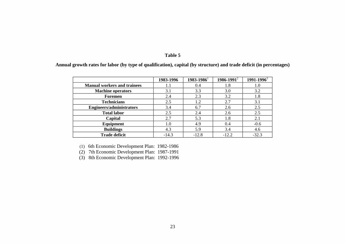
In the last decades Tunisia followed a policy of sustained capital accumulation with
an investment rate of 30% of GDP on average over the period 1981-1986. As a result
of this, the capital stock grew on average by 6.9% per year over this period compared
to 2.4% for labor. The growth rate in capital dropped to 2.4% during the adjustment
period (1987-1991) following the slowdown in investment by state enterprises. In
1992-1996 it started growing again to 2.7% per annum in the wake of the push in
investment contained in the structural adjustment program. However, the components
of capital did not always grow at a uniform rate. In 1992-1996 buildings grew by
4.8% whereas equipment declined by 1%.
Building on Ghali and Mohnen (2003), a general equilibrium model of the Tunisian
economy is used to estimate the TFP (total factor productivity) growth rate at the
sectoral and at the aggregate levels between 1983 and 1996. This TFP measure
indicates the potential of the Tunisian economy in each year of the period under
analysis and its evolution over time. It also indicates the sources of strength and of
efficiency.
Conventionally, TFP is defined as the ratio of an output index to an input index (see
Diewert (1992)). Its growth therefore represents the growth of output that goes
beyond what can be explained by the growth in the inputs. Under certain conditions,
among which constant returns to scale, optimal factor holdings and marginal cost
pricing, TFP growth as measured by the Solow residual captures the technology shift.1
It is, however, debatable whether these restrictive conditions hold. In an open
1 The Solow residual is defined as
t
t
L
t
t
K
t
t
t
t
L
LS
K
KS
Q
Q
A
A
tt
....
where K and L represent capital, labor, SK and SL their respective output elasticities, and At measures
the shift of the production function (here specified in terms of value added, Q).

3
economy it makes sense to redefine productivity as the final demand achievable with
the domestic resources and the extent of the trade deficit (Diewert and Morrison
(1986)). Another strand of literature turning around the Malmquist index distinguishes
between movements of and towards the frontier, splitting TFP growth into changes in
efficiency and changes in technology (see Caves, Christensen and Diewert (1982)).
The debate about how TFP should be measured and what it actually means is far from
being settled (see Lipsey and Carlaw (2001) for a provoking list of alternative
interpretations). We shall adopt a new approach for measuring and interpreting TFP,
entrenched in a general equilibrium model of an open economy, that does not rely on
observed market prices to infer marginal productivities, but only on the fundamentals
of the economy, i.e. technologies, preferences and endowments. The approach was
developed by ten Raa and Mohnen (2002). We apply it to the case of Tunisia for the
period 1983-1996.
We shall proceed as follows. In section II we briefly review the various measures and
interpretations of TFP. After that, in section III, we present our model of the Tunisian
economy, the calculation of the efficiency frontier and the data sources. We then turn
to the application of this model to the Tunisian economy. In section IV we analyse
Tunisia’s TFP growth first at a macro level and then at the sectoral level. We
conclude by summarizing our main findings and suggesting further lines of research.
I. The measurement and meaning of TFP
TFP has been measured and interpreted in many different ways (for some surveys, see
Diewert (1992), Balk (1998), Grosskopf (2001)). The first choice is with respect to
the number of inputs. Materials are sometimes ignored or factored out by an
assumption of separability of materials and primary inputs so that output is defined as
value-added. Each individual input might itself result from the aggregation of many
heterogeneous parts. If the input components are given the same marginal
productivities in the face of heterogeneity, we have a measurement error, akin to the
measurement error due the non-accounted for quality change. Our model has many
intermediate inputs and five different types of labor.
Most of the time TFP is measured in closed economies, ignoring possible
substitutions between domestically produced and imported inputs. In an open
economy it is possible to increase output without producing more inputs, simply by
increasing the amount of imported inputs. It is therefore important in open economy
models to adjust TFP to allow for imports, by redefining it as the growth in final
domestic demand minus the growth of the primary inputs, which include the
allowable trade deficit. As a result, TFP can now be affected by changes in the terms
of trade. TFP accounting in open economies have been handled by Diewert et
Morrison (1986) and Kohli (1991). Our model recognizes the openness of the
Tunisian economy.
In the productivity literature there are two ways to measure marginal productivities
and hence TFP. The first one is the index number approach where observed prices are
supposed to equate marginal values. The second one is the parametric approach where
4
marginal productivities are estimated from a production function or a dual
representation of it. TFP measurement in the former rests on the assumption of
constant returns to scale, optimal factor holdings and marginal cost pricing. The latter
approach in principal eschews these restrictions, although in practice it rarely happens
that all three assumptions are relaxed at the same time. On the other hand, the latter
approach requires the use of specific functional forms whereas the former approach
does not, unless it uses index numbers that are exact for specific functional forms.
A third strand of literature, starting with Farell (1957), distinguishes between
technology shifts and changes in efficiency by using the concept of a distance
function. The output distance function measures the greatest possible expansion of
output for given inputs, and the input distance function measures the greatest possible
contraction in inputs for a given output. The distance function and the resulting
Malmquist productivity index can again be obtained non-parametrically by using
linear programming techniques, known as « Data Envelopment Analysis » (DEA) or
be estimated through a stochastic frontier with an asymmetrically distributed random
error term (for a recent example of DEA and stochastic frontier analysis, see Färe,
Grosskopf, Norris and Zhang (1994) and Fuentes, Grifell-Tatjé and Perelman (2001)
resp.).
We shall depart from all four approaches : the index-number approach, the parametric
production function with technology shift specification, the DEA approach and the
estimation of a stochastic frontier specification. We follow the approach proposed by
ten Raa and Mohnen (2002), which combines input-output analysis and linear
programming. It is close in a sense to the DEA approach, except that it defines a
frontier for the entire economy, given its interrelationships in sectoral production, the
sectoral technologies, the final demand preferences and the endowments of primary
inputs. Using this approach we can follow the evolution of (in)efficiency in the use of
primary inputs and factor allocations (the distance to the frontier) and the evolution of
the production possibility frontier, in other words the potential of the Tunisian
economy.
Besides measuring correctly TFP, it is of course also rewarding to be able to explain
the fluctuations of TFP. Senhadji (1999), for instance, defines five types of
determinants : 1) the endowments in labor, capital and human capital ; 2) the terms of
trade ; 3) the macroeconomic environment ; 4) the trade regime ; and 5) the political
stability. There are many ways to decompose TFP growth. We propose two
decompositions, one in terms of the individual productivities of the primary inputs
and one in terms of changes in technologies (Solow residual), the terms of trade,
efficiency and resource utilization.
II. The model
We adopt the measure of TFP growth defined in ten Raa and Mohnen (2002) and we
apply it to the model for Tunisia used in Ghali and Mohnen (2003). The idea is to
determine the frontier of the economy by sectoral reallocation, international
specialization, and full resource utilization. For that we define a competitive
benchmark obtained by a sort of DEA analysis at the macro level. Technology,
5
preferences and factor endowments are taken as exogenous. The aim is not to
determine how the economy evolves following some kind of shock (as in computable
general equilibrium models) but simply to determine what the economy’s frontier
would be in a world of perfect competition.
On the basis of the fundamentals of the economy, i.e. the technologies, the
preferences, the endowments of labor and capital, and the world prices of tradable
commodities (because we assume that Tunisia is a small open economy), we set up a
linear programming problem or activity analysis model designed to maximize
domestic final demand given those fundamentals. For each year we solve such a linear
programming problem, which determines the optimal allocation of resources among
the various sectors of the economy, the optimal production pattern and the optimal
trade in tradable commodities. In this general equilibrium shadow prices support the
optimal quantities. In this way we trace the economy’s frontier in terms of possible
production and consumption and its evolution over time. From these optimal
quantities and shadow prices we measure potential TFP growth and we decompose it
in its constituent parts. Observed prices and quantities do not enter the TFP expression
directly. They only serve as basic inputs into the computation of the economy’s
efficiency frontier. This frontier corresponds to a hypothetical competitive world
where technology, preferences and endowments are exogenous. It corresponds thus to
a short-term optimum. Adjustment costs from the observed to the optimal allocation
of resources are not taken into account. We could conceive of a dynamic
programming problem where technologies, preferences and endowments are
endogenized with given initial conditions and with adjustment costs or other rigidities
constraining the immediate adjustment to a long-run equilibrium. We leave this
complication for future work.
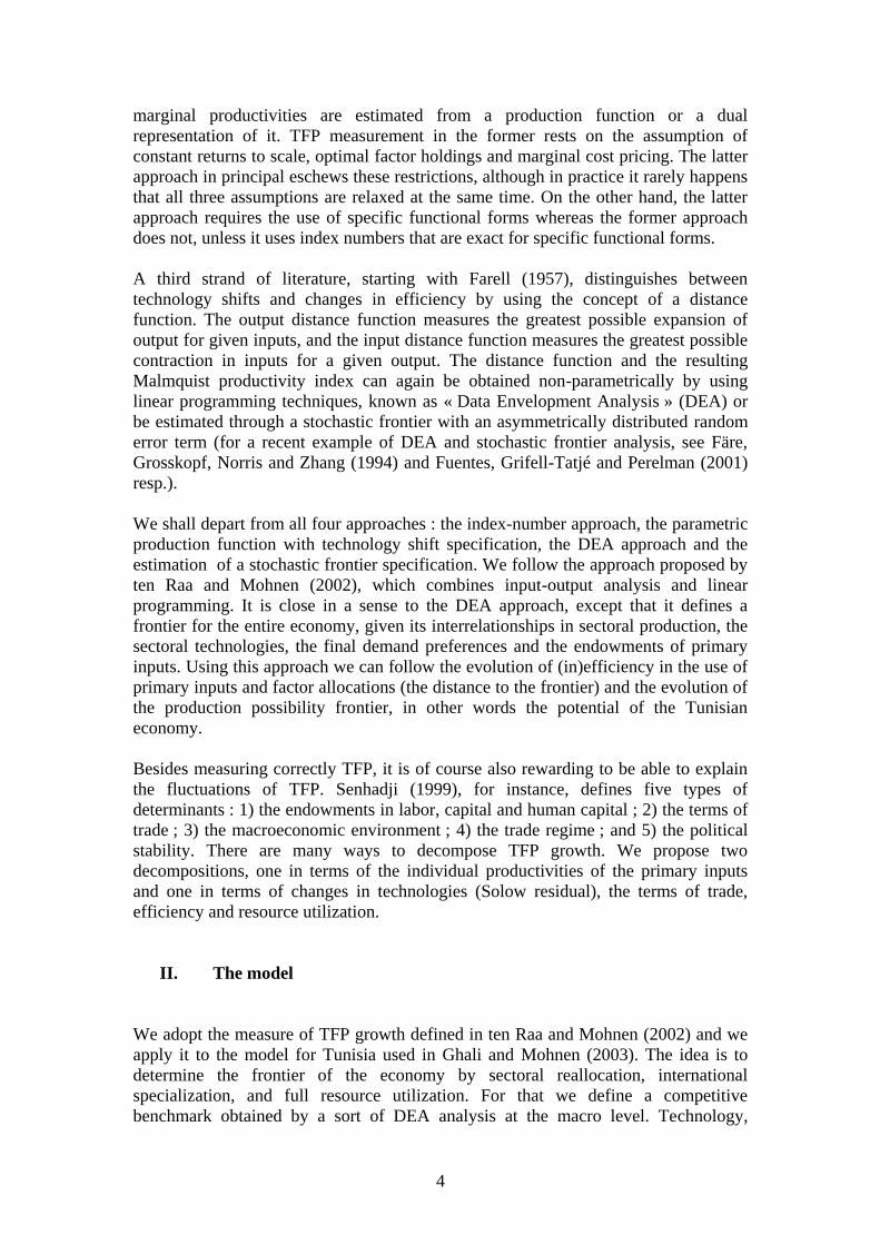
Formally, the efficient state of the economy is obtained by solving the following
linear programming problem:
tDFD
gst
)(max,,
subject to the following constraints:
JgftsUV )(' (1)
543215432154321 )()'( NNNNNtlllllsLLLLL (2)
543254325432 )()'( NNNNtllllsLLLL (3)
543543543 )()'( NNNtlllsLLL (4)
545454 )()'( NNtllsLL (5)
555NtlsL
' (6)
ee KsCK
^^
(7)
es KK ss)()(
'' (8)
Dg ' (9)
0s
Where
lwfPDFD ''~~

6
t = (Scalar) level of domestic demand;
s = (nx1) vector of activity levels, where n is the number of sectors;
g = (mT x 1) vector of net exports, where T indices tradable commodities;
V = make matrix (nxm), indicating how much of each commodity is produced in
each sector;
U = use matrix (mxn), indicating how much each commodity is used in each sector as
intermediate inputs;
J = (nxmT) matrix selecting tradables;
iL = employment of labor type i, i=1,…5, where manual workers/trainees are
indexed by 1, machine operators by 2, foremen by 3, technicians by 4, and
engineers/administrators by 5;
iN = labor force of type i, i= 1,…,5;
eK = (nx1) vector of available capital equipment stocks in each sector;
sK = (nx1) vector of available capital structure stocks in each sector;
C = (nx1) vector of capacity utilization rates in each sector;
= (mTx1) vector of world prices for tradable commodities relative to a domestic-
final-demand-weighted average of world prices;
D observed trade deficit = )( ''T
feUeV
e = unity vector of appropriate dimension; ~
P = (mx1) vector of observed commodity prices, where m is the number of
commodities;
f = ( mx1) vector of domestic final demand;
il = (5x1) vector of employment in the non-business sector for each type labor type; ~
w = (5x1) vector of observed annual labor earnings per worker by qualification in the
non-business sector;
^ = diagonalization operator.
The decision variables are the level of domestic final demand (t), the sectoral activity
levels (s) and net exports (g). They are determined so as to maximize domestic final
demand subject to three sets of constraints. The first set are the commodity balances
(1) which stipulate that net production in each sector has to be sufficient to satisfy
domestic final demand and net exports. The second set, (2) to (8), states that the
inputs used in each sector may not exceed total disposable inputs. Equipment is taken
to be sector-specific. In other words, we assume putty-clay technologies. Once
installed in one sector, equipment cannot be disassembled and affected somewhere
else. In contrast, buildings are assumed to be malleable. A sectoral capital constraint
is binding when a sector reaches full capacity utilization. For labor, we distinguish
five different types, each corresponding to a certain level of qualification and
expertise. Workers can always be affected to jobs requiring lower but not higher
qualifications. Part of the labor force is affected to the non-business sector, which
essentially comprises services directly consumed by final demand (government
services, services provided by non-profit institutions). The last constraint (9) posits
that the trade deficit at optimal activity levels may not exceed the observed trade
deficit. To increase their level of consumption, Tunisians can import from abroad, but
7
only up to a certain level, which is conservatively taken to be the observed trade
deficit. Without constraint (9), Tunisia could reach an infinite value for its objective
function by importing without limits. The assumption of a small open economy with
exogenous world prices for the tradable commodities is not unrealistic in the case of
Tunisia. The observed activity levels correspond to the following values: t=1, s=e, and
D = -’(V’e-Ue-f)T. The observed state of the economy is thus our point of reference.
Efficiency derives from full capacity utilization, optimal factor allocations across
sectors, and international specialization.
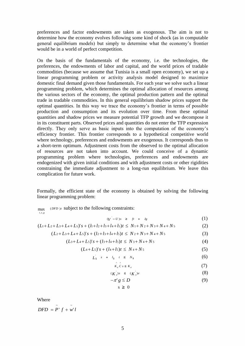
The prices sustaining this general equilibrium resource allocation are derived from the
dual program :
sconstraint following the tosubject ''min,,,
DMrNwrwp
'''')'(' KrLwUVp (10)
DFDlwfp '' (11)
'' Jp (12)
.0;0;0,012345
rwwwwwp (13)
where p, w, r and are respectively the shadow prices of commodities, of the five
types of labor, of the sectoral equipment capital stocks and the overall buildings
capital stock, and of the trade deficit2, L’ is a 5xn matrix of sectoral labor employment
by type of labor, M= ])(|['
eKK se, K= ]|[
^^
seKCK , and | is the vertical concatenation
operator. By the theorem of complementary slackness, a shadow price is positive only
if the corresponding constraint in the primal is binding. The shadow prices w and r
denote the marginal values of an additional unit of the respective inputs. If at a certain
level of qualification the labor constraint is tight, it earns a markup over the level of
qualification just below. A sector with less than full capacity utilization earns a zero
rate of return on a marginal capital investment, for the very simple reason that it is in
no excess demand, as unused capital is still available. The shadow price of the trade
balance indicates the marginal value in terms of attainable domestic final demand of
an additional allowed dinar of trade deficit. The inequalities (10) indicate that at the
optimal solution of the linear program the prices of active sectors equal average cost,
and hence that the optimal solution can be obtained as a competitive equilibrium. By
the complementary slackness conditions, it can also be said that a sector is active only
if it makes no loss. Condition (11) is a normalization condition akin to the choice of a
numeraire. At this point it should be noted that the observed prices p and w in no way
affect the optimal activity levels, they affect the shadow prices only through the
normalization rule (11), i.e. shadow prices are such that on average they reproduce the
existing prices. By equality (12) domestic prices for tradable commodities may differ
from world prices only by a certain constant , which can be interpreted as the
exchange rate compatible with the purchasing power parity. All quantities are
expressed in constant dinars, except labor, which is denoted in man-years. Hence, all
2 Notice that the shadow price of the highest qualified labor type is the sum of the shadow prices of
constraints (2) to (6).

8
shadow prices are relative constant prices, except the shadow prices of labor which
are in constant dinars per man-year.
We now turn to the definition and decomposition of TFP growth. We define TFP
growth as the growth of final demand of business and non-business goods and
services (where business goods and services refer to those for which there is an
intermediate demand) minus the growth in the primary inputs (the endowments of the
five types of labor, the sectoral capital stocks and the current trade deficit):
DMrNw
DMrNw
lwfp
lwfpTFP
''
)''(
''
)''(.....
.
(14)
where dots denotre growth rates. We can decompose TFP growth by starting from the
equality the optimal value from the primal and the optimal value of the dual, as stated
by the first theorem of linear programming :
DMrNwDFDt '' . (15)
If we totally differentiate (15), and make use of the normalization rule (11), we can
obtain, as derived by ten Raa and Mohnen (2002), that TFP growth can be written as
the sum of factor productivity growth, the weighted sum of the input prices minus a
weighted sum of the commodity prices, and efficiency change:
/])''()''(''[.......
tlwfpltwftpDMrNwTFP ( DMrNw '' ). (16)
Notice that the last term is positive if t declines, i.e. when the economy moves closer
to the efficiency frontier. We here recover a decomposition of TFP growth in terms of
movements of and towards the frontier of the economy.
By using constraints (1) to (8) and equality (11) we can decompose TFP growth in a
]})'([''
)]'([')'('])'([')'('
'''])()'[')'('{
)]''/(1[
....
......
......
.
gDgg
sKMrsKrltsLNwltsLw
tlwtfpgJpJgftUssVpUssVp
ltwftpTFP
which after simplification yields the following decomposition of TFP growth:

9
SLECTTSRTFP .
(17)
where
)]''[(/)}'(')'('){(...
ltwftpsKrsLwJgftSR
)''(/'.
ltwftpgTT
EC .
t
)]''[(/]})'([)]'(['])'(['{......
ltwftpgDsKMrltsLNwSL .
According to (17) TFP growth can be decomposed into four terms: the Solow residual
(SR), the terms of trade effect (TT) , the efficiency change effect (EC), and the change
in the slack in the use of primary inputs (SL).
The Solow residual is the traditional measure of TFP growth (value added growth
minus the growth in the conventional inputs, labor and capital), except that here it is
measured at optimal activity levels and shadow prices. The second term represents the
terms of trade effect. An appreciation in the terms of trade gives the economy the
opportunity to increase its final demand without augmenting the use of its primary
inputs. The third term is the efficiency change : a decrease in the expansion factor of
final demand implies a closer position to the efficiency frontier and translates into a
higher TFP growth. The fourth term is the change in the slack factor: an increase
[decrease] in slack, i.e. less than full resource utilization, decreases [increases] TFP
growth.
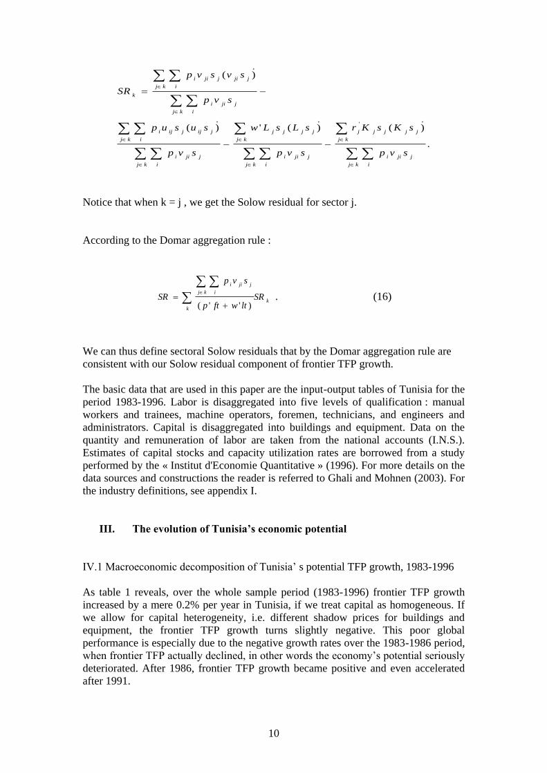
This decomposition of TFP growth, and in particular the Solow residual portion of it,
is a macroeconomic one, in a general equilibrium context. However, we can define
sectoral Solow residuals consistent with the macroeconomic Solow residual by the
Domar aggregation rule (see Hulten (1978)). Let j stand for sectors, i for
commodities, and k for groups of sectors. The Solow residual for sector-group k can
then be written as :
10
.
)()(')(
)(
'
kj i
jjii
kj
jjjjj
kj i
jjii
kj
jjjj
kj i
jjii
kj i
jijjiji
kj i
jjii
kj i
jjijjii
k
svp
sKsKr
svp
sLsLw
svp
susup
svp
svsvp
SR
Notice that when k = j , we get the Solow residual for sector j.
According to the Domar aggregation rule :
k
k
kj i
jjii
SRltwftp
svp
SR
)''( . (16)
We can thus define sectoral Solow residuals that by the Domar aggregation rule are
consistent with our Solow residual component of frontier TFP growth.
The basic data that are used in this paper are the input-output tables of Tunisia for the
period 1983-1996. Labor is disaggregated into five levels of qualification : manual
workers and trainees, machine operators, foremen, technicians, and engineers and
administrators. Capital is disaggregated into buildings and equipment. Data on the
quantity and remuneration of labor are taken from the national accounts (I.N.S.).
Estimates of capital stocks and capacity utilization rates are borrowed from a study
performed by the « Institut d'Economie Quantitative » (1996). For more details on the
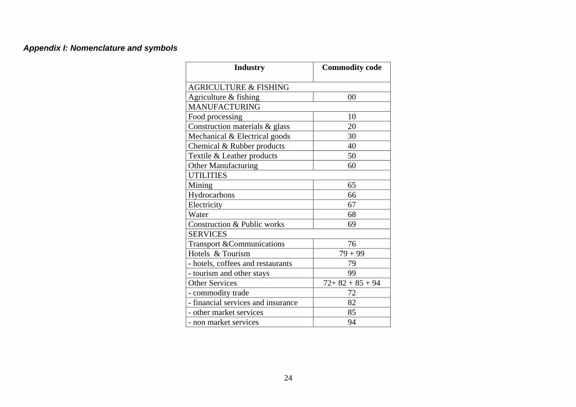
data sources and constructions the reader is referred to Ghali and Mohnen (2003). For
the industry definitions, see appendix I.
III. The evolution of Tunisia’s economic potential
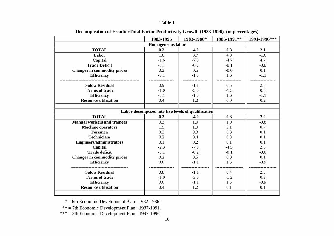
IV.1 Macroeconomic decomposition of Tunisia’ s potential TFP growth, 1983-1996
As table 1 reveals, over the whole sample period (1983-1996) frontier TFP growth
increased by a mere 0.2% per year in Tunisia, if we treat capital as homogeneous. If
we allow for capital heterogeneity, i.e. different shadow prices for buildings and
equipment, the frontier TFP growth turns slightly negative. This poor global
performance is especially due to the negative growth rates over the 1983-1986 period,
when frontier TFP actually declined, in other words the economy’s potential seriously
deteriorated. After 1986, frontier TFP growth became positive and even accelerated
after 1991.

11
The model proposes two decompositions of frontier TFP growth. The first one
decomposes it according to the marginal productivities of the individual primary
inputs. The second one decomposes it according to the variations of the exogenous
variables in the model. The results we obtain are pretty robust to the alternative
specifications on factor disaggregation: homogeneity in labor and capital,
heterogeneity in labor and homogeneity in capital, and heterogeneity in both labor and
capital. In the sequel of the paper, we report the results with five levels of labor
qualification and two types of capital stock, i.e. the bottom panel of table 1.
Regarding the input sources and beneficiaries of TFP growth, we notice that among
the workers, only manual workers and machine operators play a major role. The
action lies with the unskilled workers and not the highly skilled. The shadow price of
machine operators increased in all four subperiods, for manual workers, the least
qualified workers, it was positive in 1986-91 but dropped in the following period. The
other categories of workers contributed slightly to frontier TFP growth. From this we
can conclude that unskilled workers, especially machine operators, are the crucial
bottleneck for improved growth performance in Tunisia. The excessive wage rates for
the more qualified workers are not justified according to our activity analysis. It is a
fact that qualified labor is in excess supply in Tunisia. Highly qualified workers are
more likely to be demanded by large firms and those are few in numbers in Tunisia. In
1996, according to a study of the World Bank (World Bank (2000a), vol II, table 2.3,
p.6) 82.4% of Tunisian enterprises had less than 6 workers, while only 1.6%
employed more than 100 workers and a few dozens more than 500.
On the whole, capital, especially equipment, had a negative contribution to TFP
growth. Tunisia overinvested in equipment. This was especially so during the 1983-
1986 subperiod. The decline in equipment in 1991-1996 was beneficial to aggregate
TFP growth. The capital stock in buildings increased by 4.3% on average over the
whole period (see table 5). This increase was justified in terms of increasing potential
TFP in 1983-1986, but no more afterwards. It must be recalled that in the period
stretching from 1972 to 1985 real interest rates were negative in selected key sectors
(Morrisson and Talbi (1995), World Bank (1996)). Investment policy changed in
1987. Investment which previously had to be approved was now given financial and
fiscal incentives in some priority sectors. In 1993 a more unified code of investment
was promulgated which was based on export promotion, regional development, and
technological development. Before the structural adjustment program, the price-fixing
policy (Ghali (1995), Morrisson and Talbi (1996)), which got revised in 1986 and
then again in 1991, depressed competition in many sectors and discouraged
innovation. Protectionism was classified at level 8 out of 10 by the IMF (IMF (1999)).
The last primary input in our open model is the allowable trade deficit. Over the
whole period it played a slightly negative but modest role in frontier TFP growth
(minus one tenth of a percentage point). The marginal value in terms of domestic final
demand of an additional dinar of foreign deficit decreased over time.
We now turn to the decomposition of frontier TFP growth in terms of the growth in
the quantities of the exogenous variables. The Solow residual grew by 0.5% per year
over the whole period. In 1983-1986 it actually regressed but then it rose in the next
two sub-periods to reach an annual growth rate of 2.1% in 1991-1996. The
improvement in the Solow residual coincides with the structural adjusment program

12
started in 1987. This policy aimed at increasing competition, liberalizing prices, the
financial sector and foreign trade, reforming public enterprises, and privatizing certain
sectors like the textile and the hotel industries.
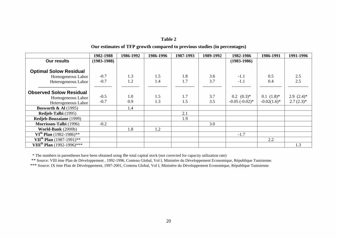
To contrast our results with other results reported in the literature, we also computed
the Solow residual at observed quantities and prices (see table 2). For that we used the
utilized capital stock as the capital input. Paquet and Robidoux (2001) have shown
with Canadian data that computing TFP growth without correcting for changes in
capacity utilization leads to a procyclical Solow residual as compared to the Solow
residual based on utilized capital stocks. To compute the observed Solow residual we
have not disaggregated the capital stock and we have calculated the user cost of
capital residually. We first notice that our observed Solow residuals are in accordance
with those reported in other studies. Only the Solow residuals implicit in the 6th to 8th
plans of economic development are somewhat out of line with our computations.
Second we notice that the optimal Solow residuals follow over time the same
movement as the observed Solow residuals but with greater variation. It is useful to
recall here that the optimal Solow residual measures the potential shift of the
production possibility frontier, whereas the usual Solow residual, evaluated at
observed prices and activity levels, measures the shift of the production function
passing through observed points.
What is striking is the strong negative effect the terms of trade exerted on frontier TFP
growth in the two sub-periods prior to 1991. In the third sub-period it turned into a
positive but minor contribution. Given the structure of Tunisia’s net exports, the
evolution of world prices was not favorable to Tunisia. On average the price of
imported goods rose more than the price of exported goods. In the end the Tunisian
economy experienced over the whole period a significant drop in its purchasing power
on world markets. The terms of trade effect almost neutralized the Solow residual
effect.
The adjustment program was successful in increasing the efficiency of the Tunisian
economy. In 1991-1996, Tunisia moved closer to its efficiency frontier. Changes in
the slacks in resource utilization played only a minor role.
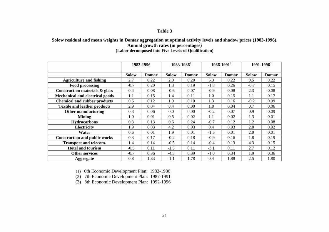
IV.2 Sectoral decomposition of Tunisia’s TFP growth, 1983-1996
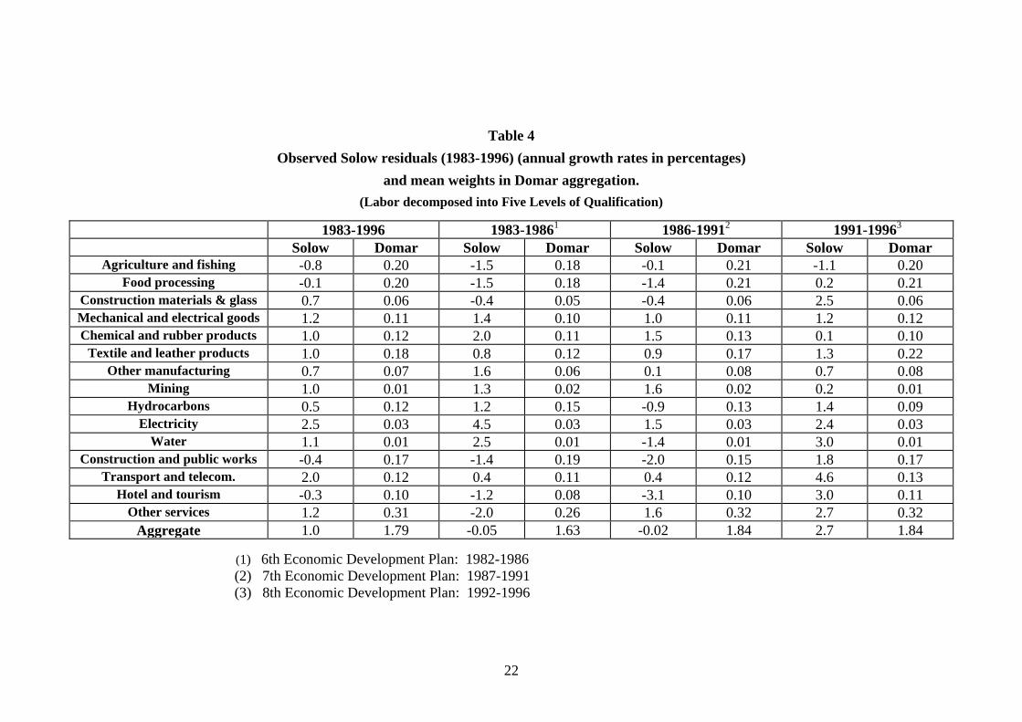
In table 3 we report the sectoral Solow residuals calculated at optimal activity levels
and shadow prices and in table 4 we report the Solow residuals calculated at observed
activity levels and prices. The observed and optimal Solow residuals follow in the
aggregate a similar evolution, but the details are quite different, and reflect the
evolution at factor scarcities. The greatest difference is visible in agriculture and
fishing. It had the high Solow residual when evaluated at optimal activity levels, but a
permanent negative Solow residual when evaluated at observed prices and quantities.
Mining had a positive (minor at the end) contribution to the observed Solow residual,
but overall a negative one with the optimal prices and quantities. Petroleum and gas,
electricity, transport and telecommunications, and other services had a strong positive
effect in both cases, even stronger at observed activity levels.

13
We also notice some significant changes in sectoral productivity performances. The
industries of construction materials, textiles and leather, petroleum and gas,
construction and public works, transport and telecommunication became more
productive in each sub-period, and hotel and tourism and other services substantially
in the last sub-period. Negative productivity trends occurred in food processing,
chemicals, mining, electricity and water utilities. Tunisia seems to be moving from a
resource-based to a services economy.
Tables 3 and 4 also give the weights used in the Domar aggregation of sectoral Solow
residuals (at optimal and observed activity levels and prices) to get to the aggregate
Solow residual. If we look at the mid sub-period, the greatest weights were attached to
other services, agriculture and fishing, construction and public works within the
utilities, and food processing within manufacturing. Observed and optimal weights
sometimes differ substantially, for example when a sector like textiles and leather
becomes inactive in the linear program. Petroleum and gas is a sector that saw a
steady decline of its importance over the sample period.
IV. Conclusion
In this study we have examined the evolution of frontier TFP in Tunisia over the
period 1983-1996 using the framework of ten Raa and Mohnen (2002). Frontier TFP
growth captures the shift in the production frontier of the economy as well as
variations in efficiency movements with respect to the frontier. The location of the
frontier is obtained by the resolution of a linear program (or activity analysis) at the
level of the whole economy, taking into account factor resource constraints, inter-
industry linkages, preferences and world prices. We have proceeded to various
decompositions of TFP growth. One decomposes it with respect to the individual
marginal productivities : capital subdivided into buildings and equipment, labor
subdivided into five levels of qualification, and the allowable trade deficit. The
second one is with respect to the exogenous variables of the model, yielding four
terms : the usual Solow residual (but evaluated at frontier quantities and supporting
prices), the terms of trade effect, the economy’s efficiency and the extent of
incomplete resource utilization.
The main results of our analysis can be summarized in the following points:
1. Over the whole sample period (1983-1996) frontier TFP growth hardly increased in
Tunisia. This poor global performance is especially due to the negative growth rates
over the 1983-1986 period, where frontier TFP actually declined, in other words the
economy’s potential deteriorated.
2. In the two sub-periods 1983-1986 and 1986-1991, corresponding to the 6th and 7th
plan of economic development, labor was the main contributor to frontier TFP
growth, and in particular machine operators. In the 1991-1996 sub-period capital (and
particularly equipment) took over from labor the positive contribution to frontier TFP
growth. The allowable trade deficit played a slightly negative but modest role in
frontier TFP growth over the whole period.
3. The Solow residual computed at frontier levels grew by 0.5% per year over the
whole period. In 1983-1986 it actually regressed but then it rose in the next two sub-

14
periods to reach an annual growth rate of 2.1% in 1991-1996. The improvement in the
Solow residual coincides with the structural adjustment program started in 1987.
What is striking is the strong negative effect the terms of trade exerted on frontier TFP
growth in the two sub-periods prior to 1991. Given the structure of Tunisia’s net
exports, the evolution of world prices was not favorable to Tunisia. In 1991-1996
Tunisia became more efficient in managing its resources.
4. Over the whole period, agriculture and fishing experienced a high Solow residual if
evaluated at optimal activity levels. The other strong performers in the frontier
allocation of resources are hydrocarbons, electricity, transport and telecommunication.
However, we also notice some significant changes in sectoral productivity
performances. The industries of construction materials, textiles and leather, petroleum
and gas, construction and public works, transport and telecommunication became
more productive in each sub-period, and hotel and tourism and other services
substantially in the last sub-period. Negative productivity trends occurred in food
processing, chemicals, mining, electricity and water utilities. Tunisia seems to be
moving from a resource-based to a services economy.
These results while suggestive of changing trends and deep restructurings in the
Tunisian economy should nevertheless be taken with some reservations. Nugent
(1970) already pointed out that activity analysis models like this one may depend
heavily on model and data imperfections. Data on capacity utilizations and labor force
by type of qualification are partly constructed and hence particularly subject to
measurement errors. Quantities are hard to measure in the service sectors and future
studies will certainly improve our measure of productivity in services. The same could
be said about quality changes with possible mismeasurement of output, especially in
high-tech commodities. It would be more rewarding to have a disagregation of labor
by skills rather than by occupations. To assume sector-specific capitals might be too
restrictive. It might be more realistic to assume different types of capital with
substitution across industries. At the other extreme it is also too restrictive to assume
perfect labor mobility. Finally, time, adjustment lags and expectations are completely
absent from this essentially static model. Introducing these elements into the model
would call for an intertemporal optimization model.

15
Bibliography
Balk, B. (1998), Industrial Price, Quantity, and Productivity Indices: The Micro-
Economic Theory and an Application. Kluwer Academic Publishers, Boston.
Barro, R. J. (1999), "Notes on Growth accounting", Journal of Economic Growth, 4,
119-137.
Ben Slama et al. (1996), “Relations technologiques intersectorielles et décomposition
des sources de la croissance”, cahiers de l’I.E.Q., no. 12.
Bosworth, B., S. Collins and Y. C. Chen (1995), "Accounting for differences in
economic growth", Brookings Discussion Papers in International Economics, No 115.
Caves, D.W., L.R. Christensen and W.E. Diewert (1982), “The economic theory of
index numbers and the measurement of input, output, and productivity”,
Econometrica, 50, 1393-1414.
De Long, J. Bradford and L. Summers (1991), “Equipment Investment and Economic
Growth”, Quarterly Journal of Economics, 106 (2), 445-502.
De Long, J. Bradford and L. Summers (1992), “Equipment Investment and Economic
Growth: How strong is the nexus.”, Brookings Papers on Economic Activity, Vol
1992 (2), 157-199.
De Long, J. Bradford and L. Summers (1993), “How Strongly do Developing
Economies Benefit from Equipment Investment ?”, Journal of Monetary Economics,
32, 395-415.
Diewert, W. E. (1976), "Exact and Superlative Index Numbers", Journal of
Econometrics, 4, 115-145.
Diewert, W. E. (1981), "The theory of total factor productivity measurement in
regulated industries", in Cowing, T. and R. Stevenson (eds.), Productivity
measurement in Regulated Industries, Academic Press, New York, 1981.
Diewert, W. E. and C.J. Morrison (1986), "Adjusting output and productivity indexes
for change in the terms of trade", Economic Journal, 96, 659-679.
Diewert, W. E. (1992), "The measurement of productivity", Bulletin of Economic
Research, 44(3), 163-198.
Domar, E. (1961), "On the measurement of technical change", Economic Journal, 70,
710-729.
Färe, R., Grosskopf S., Norris M. and Zhang Z. (1994), "Productivity growth,
Technical progress, and Efficiency change in Industrialized Countries", American
Economic Review, 84, 1, March, 66-83.
Farrell, M. J. (1957), "The measurement of productivity efficiency", Journal of Royal
Statistical Society A, 120, 253-281.
Fuentes, H.J., E. Grifell-Tatjé, and S. Perelman (2001), “A parametric distance
function approach for Malmquist productivity index estimation”, Journal of
Productivity Analysis, 15, 79-94.
Ghali, S. (1995), "Régimes des prix et organisation de la concurrence", in Schéma
Global de Développement de l'Economie Tunisienne à l' Horizon 2010, Etude
stratégique No 3, Vol III, Institut d'Economie Quantitative, Novembre.
Ghali, S. and P. Mohnen (2003), "Restructuring and Economic Performance: The
Experience of the Tunisian Economy", in Trade Policy and Economic Integration in
the Middle East and North Africa: Economic Boundaries in Flux, (Hassan Hakimian
and Jeffrey B Nugent, eds), London: Routledge-Curzon, 2003.
Griliches, Z. (1996), "The discovery of the residual: A historical note", Journal of
Economic Literature, 34, September, 1324-1330.

16
Grosskopf, S. (2001), “Some remarks on productivity and its decompositions”,
mimeo.
Hall, R.E. (1988), "Invariance properties of Solow's Residual", in Diamond, P. (ed.),
Growth / Productivity / Unemployment, M.I.T Press, Cambridge, M.A.
Hulten, C. R. (1978), "Growth accounting with intermediate inputs", Review of
Economic Studies, 45, 511-518.
Hulten, C. R. (1986), "Productivity change, capacity utilization and the sources of
efficiency growth", Journal of Econometrics, 33, 31-50.
Hulten, C. R. (1987), "Divisia Index Numbers", Econometrica, 41, 1017-1025.
Institut d’Économie Quantitative (1996), Étude stratégique No. 8, compétitivité,
restructuration, diversification et ouverture sur l’extérieur des industries
manufacturières et des services, 8622/96.
Institut National de la Statistique, Les comptes de la nation.
International Monetary Fund (1999), Tunisia: Staff Report for the Article IV
Consultation, IMF Staff Country Report No. 99/104, September, Washington D.C.
Jorgenson, D. W. and Z. Griliches (1967), "The explanation of productivity change",
Review of Economic Studies, 34(3), 308-350.
Jorgenson, D. W. and Z. Grliches (1972), "Issues in growth accounting: A reply to
Edward F. Denison", Survey of Current Business, 52, 65-94.
Kohli, U. (1991), Technology, Duality, and Foreign Trade: The GNP Function
Approach to Modeling Imports and Exports, Ann Arbor: University of Michigan
Press.
Lipsey, G. L. and K. Carlaw (2000), "What does Total Factor Productivity measure?",
International Productivity Monitor, Fall, 1, 31-40.
Morrisson, C. and B. Talbi (1996), La croissance de l’économie tunisienne en longue
période. Centre de développement de l’OCDE.
Nugent, J. (1970), “Linear programming models for national planning: demonstration
of a testing procedure”, Econometrica, 38(6), 831-855.
Paquet, A. and B. Robidoux (2001), "Issues on the measurement of the Solow residual
and the testing of its exogeneity: Evidence for Canada", Journal of Monetary
Economics, 47, 595-612.
Rama, M. (1998), "How bad is unemployment in Tunisia? Assessing labor market
efficiency in a developing country", The World Bank Research Observer, 13(1).
Redjeb, M.S. et B. Talbi (1995), "Performance de l'Economie Tunisienne durant la
Période 1961-1993", in Schéma Global de Développement de l'Economie Tunisienne
à l' Horizon 2010, Etude stratégique No 3, Vol II, Institut d'Economie Quantitative,
Novembre.
Redjeb, M. S. et L. Bouzaiane (1999), "Contribution du secteur privé à la croissance
économique en Tunisie", in L'entreprise au seuil du troisième millénaire: Défis et
Enjeux, Institut Arabe des Chefs d'Entreprises, Novembre.
Senhadji, A. (1999), "Sources of economic growth: An extensive growth accounting
exercise", I.M.F Working Paper, WP/99/77, June.
Solow, R. (1957), "Technical change and the aggregate production function", Review
of Economics and Statistics, 39, 312-320.
Ten Raa, T. and P. Mohnen (2002), " Neoclassical Growth Accounting and Frontier
Analysis : A Synthesis ", Journal of Productivity Analysis, 18, 111-128.
Wolff, E. N. (1985), "Industrial composition, interindustry effects, and the U.S
productivity slowdown", Review of Economics and Statistics, 67, 268-277.
World Bank (1996), Tunisia's global integration and sustainable development,
strategic choices for the 21. Washington D.C.

17
World Bank (2000a), Tunisia-Private sector assessment update, meeting the
challenge of globalization, report No.20173-TUN, December.
World Bank (2000b), Republic of Tunisia. Social and Structural Review 2000.
Washington D.C.
18
Table 1
Decomposition of FrontierTotal Factor Productivity Growth (1983-1996), (in percentages)
1983-1996 1983-1986* 1986-1991** 1991-1996*** Homogeneous labor
TOTAL 0.2 -4.0 0.8 2.1
Labor
Capital
Trade Deficit
Changes in commodity prices
Efficiency
-------------------------------------------------------
Solow Residual
Terms of trade
Efficiency
Resource utilization
1.8
-1.6
-0.1
0.2
-0.1
-----------------
0.9
-1.0
-0.1
0.4
3.7
-7.0
-0.2
0.5
-1.0
-----------------
-1.1
-3.0
-1.0
1.2
4.0
-4.7
-0.1
-0.0
1.6
-----------------
0.5
-1.3
1.6
0.0
-1.6
4.7
-0.0
0.1
-1.1
-----------------
2.5
0.6
-1.1
0.2
Labor decomposed into five levels of qualification
TOTAL 0.2 -4.0 0.8 2.0
Manual workers and trainees
Machine operators
Foremen
Technicians
Engineers/administrators
Capital
Trade deficit
Changes in commodity prices
Efficiency
---------------------------------------
Solow Residual
Terms of trade
Efficiency
Resource utilization
0.3
1.5
0.2
0.2
0.1
-2.3
-0.1
0.2
0.0
-----------------
0.8
-1.0
0.0
0.4
1.0
1.9
0.3
0.4
0.2
-7.0
-0.2
0.5
-1.1
-------------------
-1.1
-3.0
-1.1
1.2
1.0
2.1
0.3
0.3
0.1
-4.5
-0.1
0.0
1.5
-------------------
0.4
-1.2
1.5
0.1
-0.8
0.7
0.1
0.1
0.1
2.6
-0.0
0.1
-0.9
-------------------
2.5
0.3
-0.9
0.1
* = 6th Economic Development Plan: 1982-1986.
** = 7th Economic Development Plan: 1987-1991.
*** = 8th Economic Development Plan: 1992-1996.

19
Table 1 (con'd)
Decomposition of Total Factor Productivity Growth (1983-1996), (in percentages)
1983-1996 1983-1986* 1986-1991** 1991-1996***
Labor decomposed into five levels of qualification and capital decomposed into buildings and equipment
TOTAL -0.2 -4.7 0.8 1.6
Manual workers and trainees
Machine operators
Foremen
Technicians
Engineers/administrators
Equipment
Buildings
Trade deficit
Changes in commodity prices
Efficiency
---------------------------------------
Solow Residual
Terms of trade
Efficiency
Resource utilization
0.0
1.7
0.3
0.3
0.1
-2.1
-0.6
-0.1
0.2
0.1
-----------------
0.5
-0.6
0.1
-0.0
-0.1
1.3
0.2
0.3
0.1
-10.1
2.2
-0.1
0.6
0.9
-------------------
-2.5
-2.7
0.9
-0.2
1.6
2.2
0.3
0.3
0.2
-2.6
-2.2
-0.1
0.1
1.0
-------------------
0.6
-0.6
1.0
-0.2
-1.5
1.4
0.2
0.2
0.1
3.2
-0.6
-0.0
-0.0
-1.3
-------------------
2.1
0.6
-1.3
0.2
* = 6th Economic Development Plan: 1982-1986.
** = 7th Economic Development Plan: 1987-1991.
*** = 8th Economic Development Plan: 1992-1996.
20
Table 2
Our estimates of TFP growth compared to previous studies (in percentages)
1982-1988 1986-1992 1986-1996 1987-1993 1989-1992 1982-1986 1986-1991 1991-1996
Our results
Optimal Solow Residual Homogeneous Labor
Heterogeneous Labor
------------------------
Observed Solow Residual Homogeneous Labor
Heterogeneous Labor
(1983-1988)
-0.7
-0.7
------------
-0.5
-0.7
1.3
1.2
------------
1.0
0.9
1.5
1.4
-------------
1.5
1.3
1.8
1.7
-------------
1.7
1.5
3.6
3.7
-------------
3.7
3.5
(1983-1986)
-1.1
-1.1
-------------
0.2 (0.3)*
-0.05 (-0.02)*
0.5
0.4
---------------
0.1 (1.8)*
-0.02(1.6)*
2.5
2.5
--------------
2.9 (2.4)*
2.7 (2.3)*
Bosworth & Al (1995) 1.4
Redjeb-Talbi (1995) 2.1
Redjeb-Bouzaiane (1999) 1.9
Morrisson-Talbi (1996) -0.2 3.0
World-Bank (2000b) 1.8 1.2
VIth
Plan (1982-1986)** -1.7
VIIth
Plan (1987-1991)** 2.2
VIIIth
Plan (1992-1996)*** 1.3
* The numbers in parentheses have been obtained using the total capital stock (not corrected for capacity utilization rate)
** Source: VIII ème Plan de Développement , 1992-1996, Contenu Global, Vol I, Ministère du Développement Economique, République Tunisienne.
*** Source: IX ème Plan de Développement, 1997-2001, Contenu Global, Vol I, Ministère du Développement Economique, République Tunisienne.
21
Table 3
Solow residual and mean weights in Domar aggregation at optimal activity levels and shadow prices (1983-1996),
Annual growth rates (in percentages) (Labor decomposed into Five Levels of Qualification)
1983-1996
1983-19861 1986-1991
2 1991-1996
3
Solow Domar Solow Domar Solow Domar Solow Domar
Agriculture and fishing 2.7 0.22 2.0 0.20 5.3 0.22 0.5 0.22
Food processing -0.7 0.20 1.3 0.19 -1.8 0.26 -0.7 0.15
Construction materials & glass 0.4 0.08 -0.6 0.07 -0.9 0.08 2.3 0.08
Mechanical and electrical goods 1.1 0.15 1.4 0.11 1.0 0.15 1.1 0.17
Chemical and rubber products 0.6 0.12 1.0 0.10 1.3 0.16 -0.2 0.09
Textile and leather products 2.9 0.04 8.4 0.00 1.8 0.04 0.7 0.06
Other manufacturing 0.3 0.06 0.0 0.00 -0.2 0.07 0.9 0.09
Mining 1.0 0.01 0.5 0.02 1.1 0.02 1.3 0.01
Hydrocarbons 0.3 0.13 0.6 0.24 -0.7 0.12 1.2 0.08
Electricity 1.9 0.03 4.2 0.03 0.4 0.03 2.0 0.02
Water 0.6 0.01 1.9 0.01 -1.5 0.01 2.0 0.01
Construction and public works 0.3 0.17 -0.2 0.18 -0.9 0.16 1.8 0.19
Transport and telecom. 1.4 0.14 -0.5 0.14 -0.4 0.13 4.3 0.15
Hotel and tourism -0.5 0.11 -1.5 0.11 -3.1 0.11 2.7 0.12
Other services -0.7 0.36 -4.5 0.39 -1.0 0.34 1.9 0.36
Aggregate 0.8 1.83 -1.1 1.78 0.4 1.88 2.5 1.80
(1) 6th Economic Development Plan: 1982-1986
(2) 7th Economic Development Plan: 1987-1991
(3) 8th Economic Development Plan: 1992-1996
22
Table 4
Observed Solow residuals (1983-1996) (annual growth rates in percentages)
and mean weights in Domar aggregation.
(Labor decomposed into Five Levels of Qualification)
1983-1996 1983-19861 1986-1991
2 1991-1996
3
Solow Domar Solow Domar Solow Domar Solow Domar
Agriculture and fishing -0.8 0.20 -1.5 0.18 -0.1 0.21 -1.1 0.20
Food processing -0.1 0.20 -1.5 0.18 -1.4 0.21 0.2 0.21
Construction materials & glass 0.7 0.06 -0.4 0.05 -0.4 0.06 2.5 0.06
Mechanical and electrical goods 1.2 0.11 1.4 0.10 1.0 0.11 1.2 0.12
Chemical and rubber products 1.0 0.12 2.0 0.11 1.5 0.13 0.1 0.10
Textile and leather products 1.0 0.18 0.8 0.12 0.9 0.17 1.3 0.22
Other manufacturing 0.7 0.07 1.6 0.06 0.1 0.08 0.7 0.08
Mining 1.0 0.01 1.3 0.02 1.6 0.02 0.2 0.01
Hydrocarbons 0.5 0.12 1.2 0.15 -0.9 0.13 1.4 0.09
Electricity 2.5 0.03 4.5 0.03 1.5 0.03 2.4 0.03
Water 1.1 0.01 2.5 0.01 -1.4 0.01 3.0 0.01
Construction and public works -0.4 0.17 -1.4 0.19 -2.0 0.15 1.8 0.17
Transport and telecom. 2.0 0.12 0.4 0.11 0.4 0.12 4.6 0.13
Hotel and tourism -0.3 0.10 -1.2 0.08 -3.1 0.10 3.0 0.11
Other services 1.2 0.31 -2.0 0.26 1.6 0.32 2.7 0.32
Aggregate 1.0 1.79 -0.05 1.63 -0.02 1.84 2.7 1.84
(1) 6th Economic Development Plan: 1982-1986
(2) 7th Economic Development Plan: 1987-1991
(3) 8th Economic Development Plan: 1992-1996
23
Table 5
Annual growth rates for labor (by type of qualification), capital (by structure) and trade deficit (in percentages)
1983-1996 1983-19861 1986-1991
2 1991-1996
3
Manual workers and trainees 1.1 0.4 1.8 1.0
Machine operators 3.1 3.3 3.0 3.2
Foremen 2.4 2.3 3.2 1.8
Technicians 2.5 1.2 2.7 3.1
Engineers/administrators 3.4 6.7 2.6 2.5
Total labor 2.5 2.4 2.6 2.5
Capital 2.7 5.3 1.8 2.1
Equipment 1.0 4.9 0.4 -0.6
Buildings 4.3 5.9 3.4 4.6
Trade deficit -14.3 -12.8 -12.2 -32.3
(1) 6th Economic Development Plan: 1982-1986
(2) 7th Economic Development Plan: 1987-1991
(3) 8th Economic Development Plan: 1992-1996
24
Appendix I: Nomenclature and symbols
Industry Commodity code
AGRICULTURE & FISHING
Agriculture & fishing 00
MANUFACTURING
Food processing 10
Construction materials & glass 20
Mechanical & Electrical goods 30
Chemical & Rubber products 40
Textile & Leather products 50
Other Manufacturing 60
UTILITIES
Mining 65
Hydrocarbons 66
Electricity 67
Water 68
Construction & Public works 69
SERVICES
Transport &Communications 76
Hotels & Tourism 79 + 99
- hotels, coffees and restaurants 79
- tourism and other stays 99
Other Services 72+ 82 + 85 + 94
- commodity trade 72
- financial services and insurance 82
- other market services 85
- non market services 94