The Evidence Framework Applied to Classification Networksauthors.library.caltech.edu/13796/1/MACnc92d.pdfThe Evidence Framework Applied to Classification Networks David J. C. MacKay"

Communicated by John Bridle

The Evidence Framework Applied to Classification Networks

David J. C. MacKay" Computation and Neural Systems, California Institute of Technology, Pasadena, C A 91125 U S A

Three Bayesian ideas are presented for supervised adaptive classifiers. First, it is argued that the output of a classifier should be obtained by marginalizing over the posterior distribution of the parameters; a simple approximation to this integral is proposed and demonstrated. This involves a "moderation" of the most probable classifier's outputs, and yields improved performance. Second, it is demonstrated that the Bayesian framework for model comparison described for regression models in MacKay (1992a,b) can also be applied to classification problems. This framework successfully chooses the magnitude of weight decay terms, and ranks solutions found using different numbers of hidden units. Third, an information-based data selection criterion is derived and demonstrated within this framework.

1 Introduction

A quantitative Bayesian framework has been described for learning of mappings in feedforward networks (MacKay 1992a,b). It was demonstrated that this "evidence" framework could successfully choose the magnitude and type of weight decay terms, and could choose between solutions using different numbers of hidden units. The framework also gives quantified error bars expressing the uncertainty in the network's outputs and its parameters. In MacKay (1992~) information-based objective functions for active learning were discussed within the same framework.

These three papers concentrated on interpolation (regression) problems. Neural networks can also be trained to perform classification tasks.' This paper will show that the Bayesian framework for model comparison can be applied to these problems too.

*Current address: Darwin College, Cambridge CB3 9EU, U.K. 'In regression the target variables are real numbers, assumed to include additive

errors; in classification the target variables are discrete class labels.

Neural Computation 4,720-736 (1992) @ 1992 Massachusetts Institute of Technology

Evidence Framework Applied to Classification Networks 721

Assume that a set of candidate classification models is fitted to a data set, using standard methods. Three aspects of the use of classifiers can then be distinguished:

1. The individual classification models are used to make predictions

2. The alternative models are ranked in the light of the data.

3. The expected utility of alternative new data points is estimated for the purpose of "query learning" or "active data selection."

about new targets.

This paper will present Bayesian ideas for these three tasks. Other aspects of classifiers use such as prediction of generalizatim ability are not addressed.

First let us review the framework for supervised adaptive classification.

1.1 Derivation of the Objective Function G = Ct In p . The same notation and conventions will be used as in MacKay (1992a,b). Let the data set be D = {x(") , t,}, rn = 1 . . . N. In a classification problem, each target t , is a binary (0/1) variable [more than two classes can also be handled (Bridle 1989)], and the activity of the output of a classifier is viewed as an estimate of the probability that t = 1. It is assumed that the classification problem is noisy, that is, repeated sampling at the same x would produce different values of t with certain probabilities; those probabilities, as a function of x , are the quantities that a discriminative classifier is intended to model. It is well known that the natural objective function in this case is an information-based distance measure, rather than the sum of squared errors (Bridle 1989; Hinton and Sejnowski 1986; Hopfield 1987; Solla et al. 1988).

A classification model '?i consists of a specification of its architecture A and the regularizer R for its parameters w. When a classification model's parameters are set to a particular value, the model produces an output y (x ; w, A) between 0 and 1, which is viewed as the probability P(t = 1 1 x , w, A). The likelihood, i.e. the probability of the data' as a function of w, is then

P ( D I W, A) == Hy' ' ' ' (1 - Y)'-''~ in

= expG(D I w,A)

where

G(D Iw,A)=Ct, , logy+(1-tm)log(l-y) (1.1) m

2Strictly this is the probability of {t ,n} given {x'")}, w, A; the density over {x} is not modeled by the "discriminative" classifiers discussed in this paper.

722 David J. C. MacKay

This is the probabilistic motivation for the cross-entropy objective function Cplogq/p. Now if we assign a prior over alternative parameter vectors w,

where Ek) is a cost function for a subset (c) o f the weights and cy, is the associated regularization constant (see MacKay 1992b), we obtain a posterior:

(1.3) exp( -C,a,E$ + G)

ZM P(w 1 D , {ac}. A, R) =

where Zw and ZM are the appropriate normalizing constants. Thus the identical framework is obtained to that in MacKay (1992b) with -G re- placing the term PED. Note that in contrast to the framework for regression in MacKay (1992b) there is now no free parameter [j and no Z D ( a ) . If, however, a teacher were to supply probability estimates t instead of binary targets, then a constant equivalent to /3 would appear, expressing the precision of the teacher's estimates. This constant would correspond to the effective number of observations on which the teacher's opinion is based.

The calculation of the gradient and Hessian of G is as easy as for a quadratic E D , if the output unit's activation function is the traditional logisticf(a) = l/(l+e-'), or the generalized "softmax" in the case of more than two classes (Bridle 1989). The appropriateness of a logistic output function for a classifier is well known; it is the function that converts a log probability ratio a into a probability f ( a ) .

1.1.1 Gradient. If y[x(")'] =f[a(x("))] as defined above, the gradient of G with respect to the parameters w is

1.1.2 Hessian. The Hessian can be analytically evaluated (Bishop 1992),

VVG - Cf'g(m)gT,n, (1.5)

where f ' = Bf/aa. This approximation is expected to be adequate for the evaluation of error bars, for use in data selection and for the evaluation of the number of well-determined parameters y. A more accurate evaluation of the Hessian is probably needed for estimation of the evidence. In this paper's demonstrations, the Hessian is evaluated using second differences, i.e., numerical differentiation of VG with respect to w.

but a useful approximation neglecting terms in $a/d2w is

m


1.2 Validity of Approximations. On account of the central limit the- orem, we expect the posterior distribution to converge to a set of locally gaussian peaks with increasing quantities of data. However, the quadratic approximation to G is expected to converge more slowly than the quadratic approximation to E D , the error function for regression models, because (1) G is not a quadratic function even for a linear model [a model for which a = C W ~ $ ~ ( X ) ] : each term in G has the large scale form of a ramp function; and (2) only inputs that fall in the “bend” of the ramp contribute curvature to G. If we have the opportunity for active data selection we could improve the convergence of this quadratic approximation by selecting inputs that are expected to contribute maximal curvature. A related data selection criterion is derived in Section 4.

2 Every Classifier Should Have Two Sets of Outputs

Consider a classifier with output y(x;w) = f[a(x;w)]. Assume that we receive data D and infer the posterior probability of the parameters w (i.e., we perform ”learning”). Now if we are asked to make predictions with this classifier, it is common for the most probable parameter vector WMP to be used as the sole representative of the posterior distribution. This strategy seems unwise, however, since there may be regions in input space where the posterior ensemble is very uncertain about what the class is; in such regions the output of the network should be y N 0.5 (assuming equiprobable classes a priori), whereas typically the network with parameters WMP will give a more extreme, unrepresentative, and overconfident output. The error bars on the parameters should be taken into account when predictions are made.

In regression problems, it is also important to calculate error bars on outputs, but the problem is more acute in the case of classification because, on account of the nonlinear output, the mean output over the posterior distribution is not equal to the most probable network’s output. To obtain an output representative of the posterior ensemble of networks around WMP, we need to moderate the output of the most probable network in relation to the error bars on W M ~ .

Of course this idea of averaging over the hidden parameters is not new: marginalization goes back to Laplace. More recently, and in a con- text closer to the present one, the same message can be found for example in Spiegelhalter and Lauritzen (1990). But it seems that most practitioners of adaptive classification do not currently use marginalization.

I suggest that any classifier should have two sets of outputs. The first set would give the usual class probabilities corresponding to W M ~ , y(x; WMP); these outputs would be used for learning, i.e., for calculating the error signals for optimization of WMP. The second set would be the moderated outputs y[x;P(w I D)] = J dkwy(x;w)P(w I D); these outputs would be used for all other applications, e.g., prediction, evaluation of


test error, and for evaluating the utility of candidate data points (Sec- tion 4). Let us now discuss how to calculate the moderated outputs. It will then be demonstrated that these outputs can indeed provide better estimates of class probabilities.

2.1 Calculating the Moderated Outputs. If we assume a locally gaussian posterior probability distribution3 over w =: WMP + Aw, P(w I D ) N

P ( w M ~ ) exp( -1/2 Aw~AAw), and if we assume that the activation a(x; w) is a locally linear function of w with aa/dw = g, then for any x, the activation a is approximately gaussian distributed:

1 (a - aMP)2 P ( a ( x ) I D ) = Normal(aMP,s2) = - exp [- 2s2 ] (2.1) w

where aMP = a(x; WMP) and s2 = gTAp'g. This means that the moderated output is

P ( f = 1 1 x , D ) = .41i(aMp,s2) E daf(a)Normal(aMP,s2) (2.2) J This is to be contrasted with the most probable network's output, y(x; WMP) = f ( a M p ) . The integral of a sigmoid times a gaussian cannot be solved analytically; here I suggest a simple numerical approximation to it:

(2.3)

with IE. = l/J1+.rrS2/8. This approximation is not globally accurate over (aMp,s2), (for large s2 > a the function should tend to an error function, not a logistic) but it breaks down gracefully. The value of K was chosen so that the approximation has the correct gain at aMP = 0, as s2 -+ m. A representative of this approximation is given in Figure 1, which compares 4 and 4' with numerical evaluations of $ and I$. A similar approximation in terms of the error function is suggested in Spiegelhalter and Lauritzen (1990).

If the output is immediately used to make a (0/1) decision, then the use of moderated outputs will make no difference to the performance of the classifier (unless the costs associated with error are asymetrical), since both functions pass through 0.5 at aMp = 0. But moderated outputs will make a difference if a more sophisticated penalty function is involved. In the following demonstration the performance of a classifier's outputs is measured by the value of G achieved on a test set.

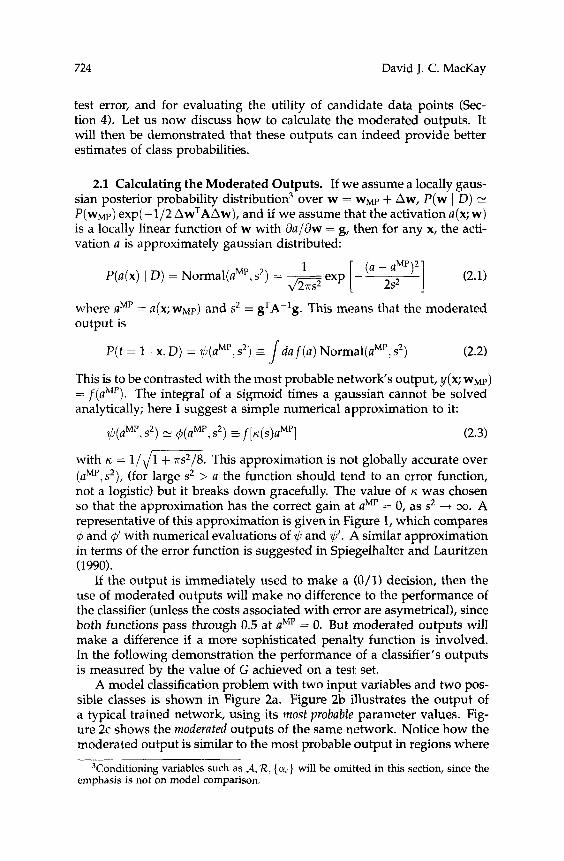
A model classification problem with two input variables and two pos- sible classes is shown in Figure 2a. Figure 2b illustrates the output of a typical trained network, using its most probable parameter values. Fig- ure 2c shows the moderated outputs of the same network. Notice how the moderated output is similar to the most probable output in regions where

$ ( a M P , s2) N 4(aMP, S*) = f[.(s)n"P]

3Conditioning variables such as A, R, {aC} will be omitted in this section, since the emphasis is not on model comparison,


Figure 1: Approximation to the moderated probability. (a) The function $(a, s2), evaluated numerically. In (b) the functions $(a, s2) and $(a, s2) defined in the text are shown as a function of a for s2 = 4. In (c), the difference 4 - $ is shown for the same parameter values. In (d), the breakdown of the approximation is emphasized by showing log$’ and log$’ (derivatives with respect to a). The errors become significant when a >> s.

the data are dense. In contrast, where the data are sparse, the moderated output becomes significantly less certain than the most probable output; this can be seen by the widening of the contours. Figure 2d shows the correct posterior probability for this problem given the knowledge of the true class densities.

Several hundred neural networks having two inputs, one hidden layer of sigmoid units and one sigmoid output unit were trained on this problem. During optimization, the second weight decay scheme of MacKay (1992b) was used, using independent decay rates for each of three weight classes: hidden weights, hidden unit biases, and output weights and biases. This corresponds to the prior that models the weights in each class as coming from a gaussian; the scales of the gaussians for different classes are independent and are specified by regularizing constants a,. Each regularizing constant is optimized on line by intermittently updating it to its most probable value as estimated within the “evidence” framework.

The prediction abilities of a hundred networks using their ”most probable’’ outputs and using the moderated outputs suggested above are compared in Figure 3. It can be seen that the predictions given by the moderated outputs are in nearly all cases superior. The improvement is most substantial for underdetermined networks with relatively poor performance. In a small fraction of the solutions however, especially among the best solutions, the moderated outputs are found to have slightly but significantly inferior performance.


Figure 2: Comparison of most probable outputs and moderated outputs. (a) The data set. The data were generated from six circular gaussian distributions, three gaussians for each class. The training sets for the demonstrations use between 100 and 1000 data points drawn from this distribution. (b) (upper right) ”Most probable” output of an eight hidden unit network trained on 100 data points. The contours are equally spaced between 0.0 and 1.0. (c) (lower left) “Moderated” output of the network. Notice that the output becomes less certain compared with the most probable output as the input moves away from regions of high training data density. (d) The true posterior probability, given the class densities that generated the data. The viewpoint is from the upper right corner of (a). In (b,c,d) a common gray scale is used, linear from 0 (dark gray) to 1 (light gray).

3 Evaluating the Evidence

Having established how to use a particular model H = {d, R} with given regularizing constants {a,} to make predictions, we now turn to the question of model comparison. As discussed in MacKay (1992a1, three levels


3600

3400

3200

3000

U

U Ll

. - Alternati+ solutions 0 -

Y‘X

/’ -

0 ,/ -

0 ,

,/b 0 0 - 0

/‘ 0 0 0

m Y

0 3 U

C

:: E U

a I:

2500 3000 3500 4000 4500 Test error for most probable parameters

Figure 3: Moderation is a good thing! The training set for all the networks contained 300 data points. For each network, the test error of the ”most probable” outputs and the “moderated” outputs were evaluated on a test set of 5000 data points. The test error is the value of G. Note that for most solutions, the moderated outputs make better predictions.

of inference can be distinguished: parameter estimation, regularization constant determination, and model c~mpar ison .~ The second two levels of inference both require “Occam’s razor”; that is, the solution that best fits the data is not the most plausible model, and we need a way to balance goodness of fit against complexity. Bayesian inference embodies such an Occam’s razor automatically.

At the first level, a model ‘FI, with given regularizing constants {a,}, is fitted to the data D. This involves inferring what value the parameters w should probably have. Bayes‘ rule for this level of inference has the form:

Throughout this paper this posterior is approximated locally by a gaussian:

where Aw = w - w M ~ , M(w) = Cco,Ef - G, and A = VVM.

4The use of a specified model to predict the class of a datum can be viewed as the zeroeth level of inference.

728 David J. C . MacKay

At the second level of inference, the regularizing constants are optimized:

The data-dependent term P(D I {ac}, Y) is the “evidence,” the normalizing constant from equation 3.1. The evaluation of this quantity and the optimization of the parameters {a,} is accomplished using a framework due to Gull and Skilling, discussed in detail in MacKay (1992a,b).

Finally, at the third level of inference, the alternative models are compared:

(3.4)

Again, the data’s opinion about the alternatives is given by the evidence from the previous level, in this case P(D I 3-1).

Omitting the details of the second level of inference, since they are identical to the methods in MacKay (1992b), this demonstration presents the final inferences, the evidence for alternative solutions. The evidence is evaluated within the gaussian approximation from the properties of the ”most probable” fit WMP, and the error bars A-’, as described in MacKay (1 992a).

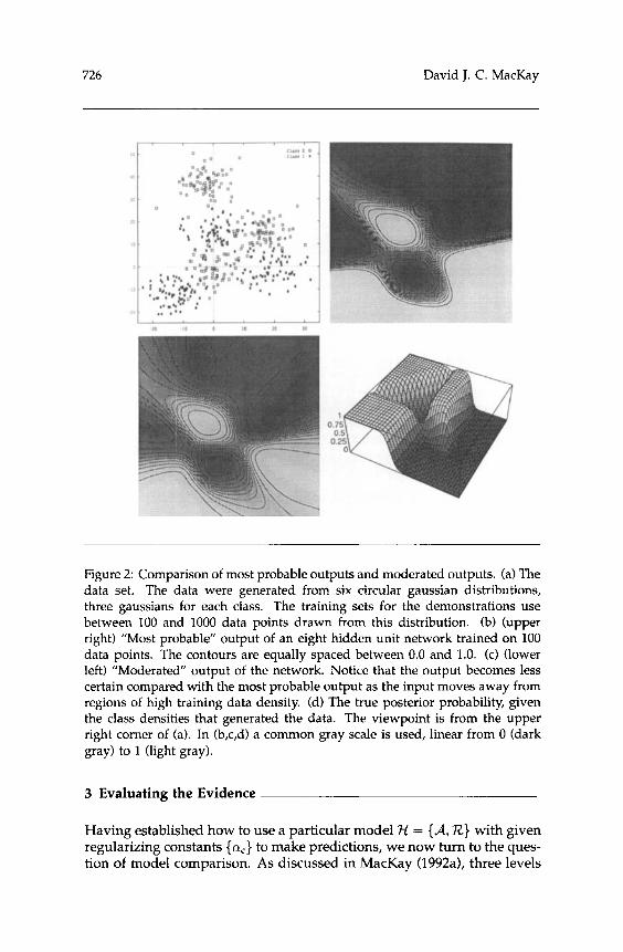
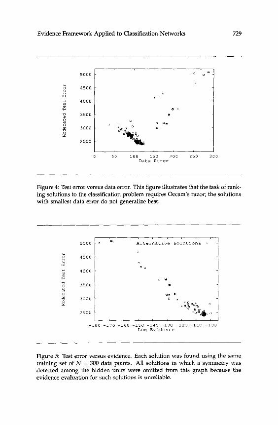
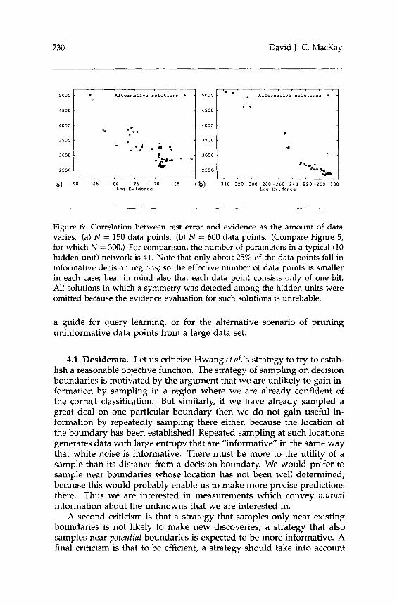
Figure 4 shows the test error (calculated using the moderated outputs) of the solutions against the data error, and the ”Occam’s razor” problem can be seen: the solutions with smallest data error do not generalize best. Figure 5 shows the log evidence for the solutions against the test error, and it can be seen that a moderately good correlation is obtained. The correlation is not perfect. It is speculated that the discrepancy is mainly due to inaccurate evaluation of the evidence under the quadratic approximation, but further study is needed here. Finally, Figure 6 explores the dependence of the correlation between evidence and generalization on the amount of data. It can be seen that the correlation improves as the number of data points in the test set increases.

pm I D) 0; w I 3-1)P(3-1)

4 Active Learning

Assume now that we have the opportunity to select the input x where a future datum will be gathered (“query learning”). Several papers have suggested strategies for this active learning problem, for example, Hwang etal. (1991) propose that samples should be made on and near the current decision boundaries. This strategy and that of Baum (1991) are both human-designed strategies and it is not clear what objective function if any they optimize, nor is it clear how the strategies could be improved. In this paper, as in MacKay (199213, the philosophy will be to derive a criterion from a defined sensible objective function that measures how useful a datum is expected to be. This criterion may then be used as


5000

2 4 5 0 0 U W

u 4000

01 H

p 3 5 0 0 u U $ 3 0 0 0

s 2 5 0 0

- a D o -

-

-

810

- U

0 O P -

-

Figure 4: Test error versus data error. This figure illustrates that the task of rank- ing solutions to the classification problem requires Occam’s razor; the solutions with smallest data error do not generalize best.

5 0 0 0

U 4 5 0 0

U W

CI

m H

vl 4 0 0 0

2 3 5 0 0 u U m U 3 0 0 0 B

2 5 0 0

- 0 % Alternative solutions 0 -

-

0 0 -

o m

- a

BJO

- 0 0

.%..., 0

- n.%& -

Figure 5: Test error versus evidence. Each solution was found using the same training set of N = 300 data points. All solutions in which a symmetry was detected among the hidden units were omitted from this graph because the evidence evaluation for such solutions is unreliable.


4500

4000

3500

3000

2500

L I D t

a) -90 -85 -80 - 7 5 -10 -65 -6b) -340 -320 -300 -280 -260 -240 -220 -200 -100 Log Evldence Lag Evidence

Figure 6: Correlation between test error and evidence as the amount of data varies. (a) N = 150 data points. (b) N = 600 data points. (Compare Figure 5, for which N = 300.) For comparison, the number of parameters in a typical (10 hidden unit) network is 41. Note that only about 25% of the data points fall in informative decision regions; so the effective number of data points is smaller in each case; bear in mind also that each data point consists only of one bit. All solutions in which a symmetry was detected among the hidden units were omitted because the evidence evaluation for such solutions is unreliable.

a guide for query learning, or for the alternative scenario of pruning uninformative data points from a large data set.

4.1 Desiderata. Let us criticize Hwang et al.'s strategy to try to estab- lish a reasonable objective function. The strategy of sampling on decision boundaries is motivated by the argument that we are unlikely to gain information by sampling in a region where we are already confident of the correct classification. But similarly, if we have already sampled a great deal on one particular boundary then we do not gain useful information by repeatedly sampling there either, because the location of the boundary has been established! Repeated sampling at such locations generates data with large entropy that are "informative" in the same way that white noise is informative. There must be more to the utility of a sample than its distance from a decision boundary. We would prefer to sample near boundaries whose location has not been well determined, because this would probably enable us to make more precise predictions there. Thus we are interested in measurements which convey mutual information about the unknowns that we are interested in.

A second criticism is that a strategy that samples only near existing boundaries is not likely to make new discoveries; a strategy that also samples near potential boundaries is expected to be more informative. A final criticism is that to be efficient, a strategy should take into account

Evidence Framework Applied to Classification Networks 73 1

how influential a datum will be: some data may convey information about the discriminant over a larger region than others. So we want an objective function that measures the global expected informativeness of a datum.

4.2 Objective Function. This paper will study the "mean marginal information." This objective function was suggested in MacKay (1992~1, and a discussion of why it is probably more desirable than the joint information is given there. To define this objective function, we first have to define a region of interest. (The objective of maximal information gain about the model's parameters without a region of interest would lead us to sample at unsampled extremes of the input space.) Here this region of interest will be defined by a set of representative points x('), u = 1 . . . V, with a normalized distribution P, on them. P, can be interpreted as the probability that we will be asked to make a prediction at x('). [The theory could be worked out for the case of a continuous region defined by a density p(x), but the discrete case is preferred since it relates directly to practical implementation.] The marginal entropy of a distribution over w, P(w), at one point x(,) is defined to be

(4.1)

where y, = y[x(");P(w)] is the average output of the classifier over the ensemble P(w). Under the gaussian approximation for P(w), y, is given by the moderated output (equation 2.2), and may be approximated by @(a:', s!) (equation 2.3).

s i ) = yu logy, + (1 - y u ) log(1 - yu)

The mean marginal entropy is

The sampling strategy studied here is to maximize the expected change in mean marginal entropy. (Note that our information gain is minus the change in entropy.)

4.3 Estimating Marginal Entropy Changes. Let a measurement be made at x. The result of this measurement is either t = 1 or t = 0. Assuming that our current model, complete with gaussian error bars, is correct, the probability of t = 1 is $[uMp(x), s2(x)] 11 @(aMP, s2). We wish to estimate the average change in marginal entropy of t , at x(") when this measurement is made.

This problem can be solved by calculating the joint probability distribution Pjt, tu ) of t and f,, then finding the mutual information between the two variables. The four values of P ( t , t,) have the form

P(t=l,t,=l)=//dada,f(a)f(a,)-exp Z


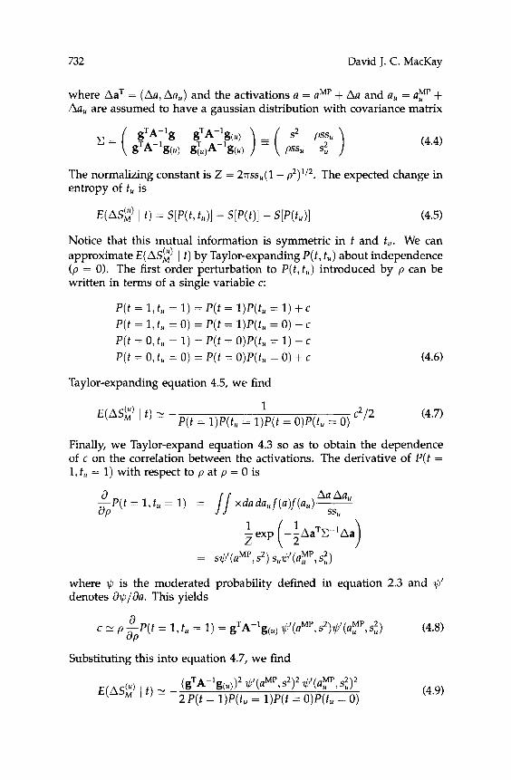
where AaT = (Aa, Aa,) and the activations a = aMP + Aa and a, = ayp + Aa, are assumed to have a gaussian distribution with covariance matrix

(4.4)

The normalizing constant is Z = 2nss,(l - p2)1/2. The expected change in entropy of t, is

E ( A S ~ ) I t ) = q q t , t,)] - S[P(~)I - sp(t,)l (4.5)

Notice that this mutual information is symmetric in t and t,. We can approximate E( Ask) I t) by Taylor-expanding P( t , t,) about independence (p = 0). The first order perturbation to P(t , t , ) introduced by p can be written in terms of a single variable c:

P ( t = 1, t, = 1) = P ( t = l)P(t, = 1) + c P ( t = 1, t, = 0) = P(t = l)P(t, = 0) - c P ( t = 0, t, = 1) = P(t = O)P(t , = 1) - c P ( t = 0, t, = 0) = P ( t = O)P(t, = 0) + c

Taylor-expanding equation 4.5, we find

c2/2 1 E ( A S ~ ) I t ) 21 - P ( t = l)P(t, = l)P(t = O)P(t, = 0)

(4.6)

(4.7)

Finally, we Taylor-expand equation 4.3 so as to obtain the dependence of c on the correlation between the activations. The derivative of P(t = 1, t, = 1) with respect to p at p = 0 is

d Aa aa, -P(t = l , t , = 1) = 11 xdada,f(a)f(a,)--- &J ss,

MI' 2 MP 2 = s$'(a , s ) s,?ll(au rsu)

where $ is the moderated probability defined in equation 2.3 and $' denotes a$/&. This yields

(4.8) c N p ,P(t a = 1, t, = 1) = gTA-'gcu, $'(aMp, S ~ ) $ ( U , MP , s,) 2 dP

Substituting this into equation 4.7, we find

(gTA-'g(,,))' $'(aMP, s ' )~ $'(UYI', ~ 2 ) ~ E ( A S ~ ) 1 t ) = - 2P(t = l)P(tU = l)P(t = O)P(t, = 0) (4.9)


Assuming that the approximation $ 'v q!~ 5 f [ ~ ( s ) a ~ ' ] is good, we can numerically approximate d$(uMP, s')/13u by K ( s ) ~ ' [ K ( s ) u ~ " ] . ~ Using f ' = f(1 - f ) we obtain

E(AS&) I f) N - K ( s ) ~ ~ ; ( s , ) ' ~ ' [ K ( s ) u MP I f / [ K ( s , ) u ~ ~ " ] (gTA-'g[,))'/2 (4.10)

The two f ' terms in this expression correspond to the two intuitions that sampling near decision boundaries is informative, and that we are able to gain more information about points of interest if they are near boundaries. The term (gTA-'g[,))' modifies this tendency in accordance with the desiderata.

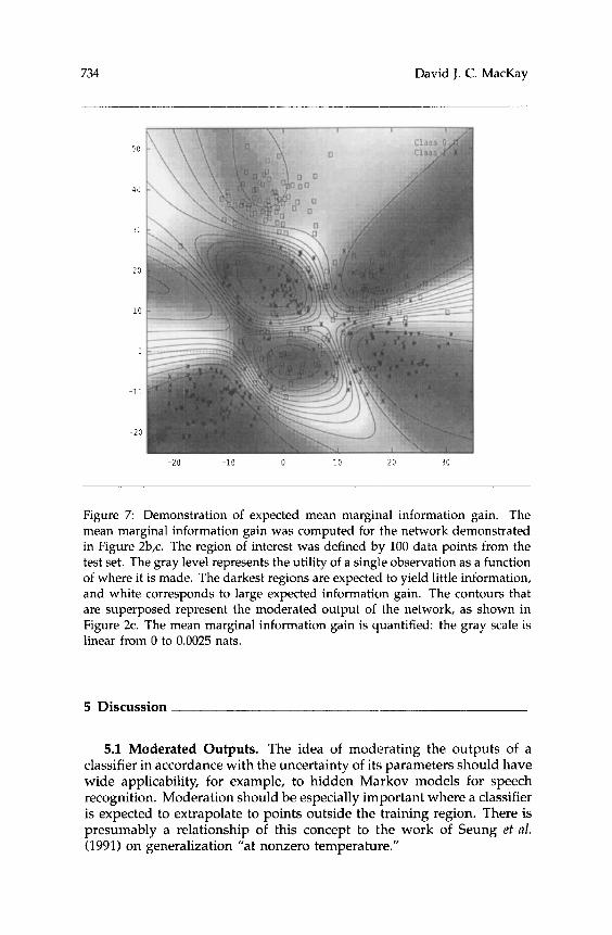
The expected mean marginal information gain is computed by adding up the Ask's over the representative points x(I0. The resulting function is plotted on a grey scale in Figure 7, for the network solving the toy problem described in Figure 2. For this demonstration the points of interest x(I1) were defined by drawing 100 input points at random from the test set. A striking correlation can be seen between the regions in which the moderated output is uncertain and regions of high expected information gain. In addition the expected information gain tends to increase in regions where the training data were sparse.

Now to the negative aspect of these results. The regions of greatest expected information gain lie outside the region of interest to the right and left; these regions extend in long straight ridges hundreds of units away from the data. This estimation of utility, which reveals the "hyperplanes" underlying the model, seems unreasonable. The utility of points so far from the region of interest, if they occurred, could not really be so high. There are two plausible explanations of this. It may be that the Taylor approximations used to evaluate the mean marginal information are at fault, in particular equation 4.8. Or as discussed in MacKay (19923, the problem might arise because the mean marginal information estimates the utility of a point assuming that the model is true; if we assume that the classification surface really can be described in terms of hyperplanes in the input space, then it may be that the greatest torque on those planes can be obtained by sampling away from the core of the data. Comparison of the approximation 4.10 with numerical evaluations of AS&) indicates that the approximation is never more than a factor of two wrong. Thus the latter explanation is favored, and we must tentatively conclude that the mean marginal information gain is likely to be most useful only for models well matched to the real world.

5This approximation becomes inaccurate where uMP >> s >> 1 (see Fig. lc). Because of this it might be wise to use numerical integration then implement AS:) in look-up tables.


3 0 2 0 1 0 0 -10 - 2 0

Figure 7 Demonstration of expected mean marginal information gain. The mean marginal information gain was computed for the network demonstrated in Figure 2b,c. The region of interest was defined by 100 data points from the test set. The gray level represents the utility of a single observation as a function of where it is made. The darkest regions are expected to yield little information, and white corresponds to large expected information gain. The contours that are superposed represent the moderated output of the network, as shown in Figure 2c. The mean marginal information gain is quantified: the gray scale is linear from 0 to 0.0025 nats.

5 Discussion

5.1 Moderated Outputs. The idea of moderating the outputs of a classifier in accordance with the uncertainty of its parameters should have wide applicability, for example, to hidden Markov models for speech recognition. Moderation should be especially important where a classifier is expected to extrapolate to points outside the training region. There is presumably a relationship of this concept to the work of Seung et al. (1991) on generalization ”at nonzero temperature.”


If the suggested approximation to the moderated output and its derivative is found unsatisfactory, a simple brute force solution would be to set up a look-up table of values of +(a,s2) and +'(u,s2).

It is likely that an implementation of marginalization that will scale up well to large problems will involve Monte Carlo methods (Neal 1992).

5.2 Evidence. The evidence has been found to be well correlated with generalization ability. This depends on having a sufficiently large amount of data. There remain open questions, including what the theoretical relationship between the evidence and generalization ability is, and how large the data set must be for the two to be well correlated, how well these calculations will scale up to larger problems, and when the quadratic approximation for the evidence breaks down.

5.3 Mean Marginal Information Gain. This objective function was derived with active learning in mind. It could also be used for selection of a subset of a large quantity of data, as a filter to weed out fractions of the data that are unlikely to be informative. Unlike Plutowski and White's (1991) approach this filter depends only on the input variables in the candidate data. A strategy that selectively omits data on the basis of their output values would violate the likelihood principle and risk leading to inconsistent inferences.

A comparison of the mean marginal information gain in Figure 7 with the contours of the most probable networks output in Figure 2b indicates that this proposed data selection criterion offers some improvements over the simple strategy of just sampling on and near decision boundaries: the mean marginal information gain shows a plausible preference for samples in regions where the decision boundary is uncertain. On the other hand, this criterion may give artifacts when applied to models that are poorly matched to the real world. How useful the mean marginal information gain will be for real applications remains an open question.

Acknowledgments

This work was supported by a Caltech Fellowship and a Studentship from SERC, UK.

References

Baum, E. 8. 1991. Neural net algorithms that learn in polynomial time from

Bishop, C. M. 1992. Exact calculation of the Hessian matrix for the multilayer examples and queries. I E E E Truns. Neurul Networks 2(1), 5-19.

perceptron. Neurul Comp. 4(4), 494-501.


Bridle, J. S. 1989. Probabilistic interpretation of feedforward classification network outputs, with relationships to statistical pattern recognition. In Neuro- computing: Algorithms, Architectures and Applications, F. Fougelman-Soulie and J. Hkrault, eds., pp. 227-236. Springer-Verlag, Berlin.

Hinton, G. E., and Sejnowski, T. J. 1986. Learning and relearning in Boltzmann machines. In Parallel Distributed Processing, Rumelhart et al., eds., pp. 282- 317. The MIT Press, Cambridge.

Hopfield, J. J. 1987. Learning algorithms and probability distributions in feedforward and feed-back networks. Proc. Natl. Acad. Sci. U.S.A. 84,8429-8433.

Hwang, J-N., Choi, J. J., Oh, S., and Marks, R. J., I1 1991. Query-based learning applied to partially trained multilayer perceptrons. IEEE Trans. Neural Networks 2(1), 131-136.

MacKay, D. J. C. 1992a. Bayesian interpolation. Neural Comp. 4(3), 415-447. MacKay, D. J. C. 1992b. A practical Bayesian framework for backprop networks.

Neural Comp. 4(3), 448-472. MacKay, D. J. C. 1992~. Information-based objective functions for active data

selection. Neural Comp. 4(4), 589-603. Neal, R. M. 1992. Bayesian training of backpropagation networks by the Hybrid

Monte Carlo Method. University of Toronto CRG-TR-92-1. Plutowski, M., and White, H. 1991. Active selection of training examples for net-

work learning in noiseless environments. Dept. Computer Science, UCSD,

Seung, H. S., Sompolinsky, H., and Tishby, N. 1991. Statistical mechanics of

Solla, S. A., Levin, E., and Fleisher, M. 1988. Accelerated learning in layered

Spiegelhalter, D. J., and Lauritzen, S. L. 1990. Sequential updating of conditional

TR 90-011.

learning from examples. Preprint, Racah Institute of Physics, Israel.

neural networks. Complex Syst. 2, 625-640.

probabilities on directed graphical structures. Networks 20, 579-605.

~~

Received 20 November 1991; accepted 18 February 1992.

Documents

The Evidence Framework Applied to Classification Networksauthors.library.caltech.edu/13796/1/MACnc92d.pdfThe Evidence Framework Applied to Classification Networks David J. C. MacKay"