Embed Size (px)
Citation preview
The Evaluation of Fisheries Management: A DynamicStochastic Approach†
Jose M. Da-Rocha
RGEA - Universidade de Vigo (Spain) and ITAM (Mexico)
Marıa-Jose Gutierrez
DFAEII, University of the Basque Country (Spain)
March 2008
Abstract
Most existing studies evaluating the management of fisheries fail to reproduce the
observed dynamics of the resource. We present an alternative approach: assuming that
the stock growth path is affected by productivity shocks that follow a Markov process, we
calibrate the growth path of the resource such that the observed dynamics of resource are
matched. In this context, an efficient policy consists of applying a different exploitation rule
depending on the state of the resource and the constant-escapement rule is not the efficient
policy.
Keywords : Fisheries Management, Renewable Resources, Calibration, Biomass Dynamics
JEL Classification: Q22, Q28.
†Financial support from the ERDF, Fundacion BBVA, Spanish Ministry of Science and Technology and
University of the Basque Country is acknowledged.
Contact Information: Marıa-Jose Gutierrez. Universidad del Paıs Vasco. Avda. Lehendakari Aguirre, 83.
48015 Bilbao. Spain. Fax: (34) 946013786. e-mail: [email protected].
1 Introduction
Efficiency in managing the exploitation of fishery resources has been widely analyzed in
resource literature.1 In general terms, these studies only focus on show how far is the optimal
steady state values of biomass and catches from the observed path, and the goodness of the
bioeconomic model used to reproduce the observed dynamics of the resource and catches is
never checked. However, we think that good reproduction of the observed data is a minimum
condition that any fishery assessment study must satisfy. In particular, we believe that the
better the model reproduces the observed evolution of the biomass the more reliable the
assessment of the exploitation is.
In this paper we present an alternative approach that allows us reproduce better the
stylized facts of the fishing ground. This is a stochastic approach in which we assume that
the stock growth path is affected by stochastic productivity shocks that follow a Markov
process.2 We calibrate the growth path of the resource to match the observed dynamics of
the resource and captures. This approach is very well known and developed in other economic
areas, but it is harddly used in natural resources economics.3 As far as we know only Singh,
Weninger and Doyle (2006) uses a similar stochastic technique to analyze numerically the
importance of costly capital adjustment in fishery models with random stock growth.
With this kind of approach, we do not limit our work to comparing the observed paths
of captures and biomass with the stationary values from a deterministic model. Our analysis
goes further into the calculations of the optimal exploitation rules associated with both the
size and the productivity of the biomass. Summarizing, with productivity shocks affecting
the growth of the biomass, an efficient policy consists of applying a different exploitation
rule depending on the state of the resource, and we could say that the stock is always in
transition, jumping from one steady state to another.
This stochastic approach is applied to the European Southern Stock of Hake (ESSH).
We study this fishing grounds for three reasons. First, it is considered as individual admin-
1Among others, Garza-Gil et al. (2003), Del Valle et al. (2001), Grafton et al. (2000), Garza-Gil (1998),
Flaaten and Stollery (1996), Amundsen et al. (1995)).2Productivity shocks can reflect that the biomass may be affected by biological cycles (Larraneta and
Vazquez (1982)) or any other ecological uncertainty element.3Kydland and Prescott (1982) can be considered as the pioneer article in aplying the calibration technique
to evaluate macroeconomic models in quantitative manner.
2
istrative units by the International Council for the Exploitation of the Sea (ICES), which
advises the European Commission on their management. Second, it has been analyzed pre-
viously by Garza-Gil (1998) with the traditional approach. This previous research allow us
to focus on the calibration of the growth resource because it shows information about cap-
turability functions, prices of captures and costs of effort. Third, biomass evolution shows
a monotonic (dramatically) descending trend and the ICES recommends a recovery plan to
ensure safe and rapid rebuilding.
Our results show that in aggregate terms, catches have been even lower than would cor-
respond to efficient exploitation. However, the timing of captures has not been appropriate
and the exploitation has not been able to protect the resource. This inefficiency has meant
a reduction of potential profits by 35% in the fishery. Moreover the ESSH is in a dangerous
situation; in particular, our results show that an efficient exploitation policy would bring
the stock up to ICES recommended levels. We also illustrate how captures should be shared
between the two existing fleets once the fishing ground is recovered. Our results indicate
that efficient exploitation will require a larger proportion of the total captures to go to the
artisanal fleet than is currently the case.
Other authors have introduced uncertainty into the dynamics of the resource. An-
drokovich and Stollery (1989) simulate a stochastic dynamic program to quantify the rel-
ative merits of different policies for regulating the Pacific halibut fishery. More recently,
Danielsson (2002) and Weitzman (2002) analyze the relative performance of different meth-
ods of fisheries management when there are some risks involved. Both include “ecological”
or “environmental” uncertainty in the biological dynamics of the fish stock. Sethi, Costello,
Fisher, Hanemann and Karp (2005) develop a theoretical model that incorporates uncer-
tainty about, among others, variability in fish dynamics assuming Markovian transitions.
Our work is on the same line as these studies; in particular we assume that the current state
of productivity may depend on past productivity.
The paper proceeds as follows. In the next section the traditional approach to the
evaluation of fisheries management is presented. In particular, we show with an example how
poorly this approach may reproduce the observed dynamics of the biomass. In Section 3 an
alternative stochastic approach is proposed. First a multifleet fishery model with stochastic
biomass dynamics is developed, and secondly, a method for calibrating the growth path of
3
the resource is proposed. The model is adapted to characterize the ESSH fishery in Section
4. Subsection 4.1 presents the calibration of the fishing ground and in Subsection 4.2 assess
fishery management and reports what would have happened if side-payments between fleets
had been allowed. Section 6 concludes the paper with a policy recommendation discussion.
2 The Traditional Approach
The literature of fishery efficiency assessment has traditionally followed a deterministic steady
state approach that considers that an efficient policy consists of maintaining the exploitation
levels of the fishing ground at steady state values. In this section we show the effects that
this approach may have on the expected evolution of the resource.
Let us consider that the stock of the fishing ground we want to evaluate, Xt, is char-
acterized by the following dynamics
Xt+1 = F (Xt)− Yt, (1)
where Yt is total catches and F is the gross growth of the biomass, which depends upon the
stock of resource, Xt.
The traditional approach consists of the following steps: i) The dynamics of the resource
are estimated using data on stock and captures, ii) An appropriate parametric form for the
gross growth of the stock, F , is selected based on this estimation, iii) The complete theoretical
problem is solved4, and iv) Parameters estimated in steps i) and ii) are used to evaluate the
fishery according to the solution of the theoretical model. The problem of this procedure is
that the estimated dynamics of the resource (step i) ) are never checked against the data
used to estimate them. That means that we may be using an estimation for evaluation which
may be inappropriate. We show an example of this effect.
Let us consider the ESSH for the period 1982-20025. Our estimation results point to
the Ricker as being the functional form that best fits the data of this fishery.6 The traditional
approach would use the estimation of the parameters of this functional form to evaluate the
4Other functional forms such as capturability and profit functions are usually involved in
the theoretical problem.5Data used are shown in Table 4 in Appendix A.6We show how this selection is made in section 4.1.
4
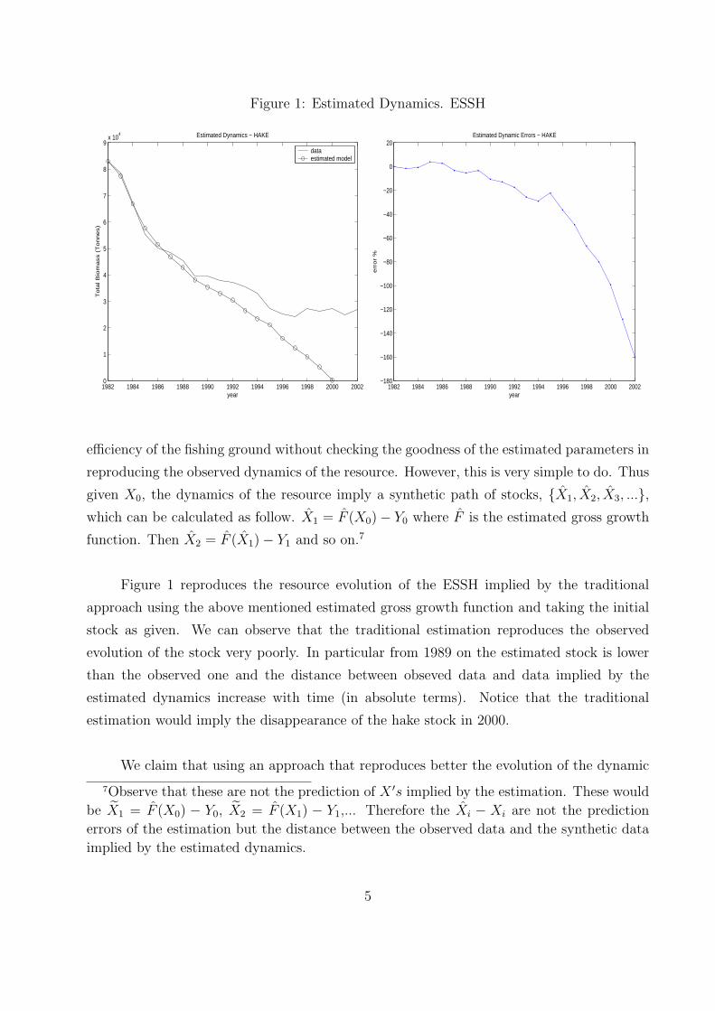
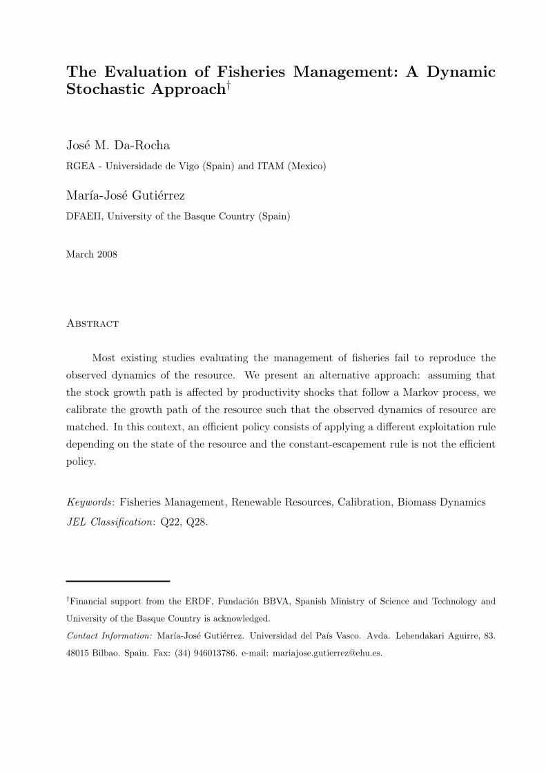
Figure 1: Estimated Dynamics. ESSH
1982 1984 1986 1988 1990 1992 1994 1996 1998 2000 20020
1
2
3
4
5
6
7
8
9x 10
4 Estimated Dynamics − HAKE
year
To
tal B
iom
ass (
To
nn
es)
dataestimated model
1982 1984 1986 1988 1990 1992 1994 1996 1998 2000 2002−180
−160
−140
−120
−100
−80
−60
−40
−20
0
20Estimated Dynamic Errors − HAKE
year
err
or
%
efficiency of the fishing ground without checking the goodness of the estimated parameters in
reproducing the observed dynamics of the resource. However, this is very simple to do. Thus
given X0, the dynamics of the resource imply a synthetic path of stocks, {X1, X2, X3, ...},which can be calculated as follow. X1 = F (X0)− Y0 where F is the estimated gross growth
function. Then X2 = F (X1)− Y1 and so on.7
Figure 1 reproduces the resource evolution of the ESSH implied by the traditional
approach using the above mentioned estimated gross growth function and taking the initial
stock as given. We can observe that the traditional estimation reproduces the observed
evolution of the stock very poorly. In particular from 1989 on the estimated stock is lower
than the observed one and the distance between obseved data and data implied by the
estimated dynamics increase with time (in absolute terms). Notice that the traditional
estimation would imply the disappearance of the hake stock in 2000.
We claim that using an approach that reproduces better the evolution of the dynamic
7Observe that these are not the prediction of X ′s implied by the estimation. These would
be X1 = F (X0) − Y0, X2 = F (X1) − Y1,... Therefore the Xi − Xi are not the prediction
errors of the estimation but the distance between the observed data and the synthetic data
implied by the estimated dynamics.
5
resource leads to more reliable results in evaluating the efficiency of resource management.
3 A Stochastic Approach
In this section a new stochastic approach is presented to evaluate the efficiency of fishing
resource management. Firstly, we present a multifleet bioeconomic model in which the
resource is affected by stochastic productivity shocks. Secondly, since the model has to be
simulated, we describe how to calibrate it, i.e. how to choose values for the parameters that
reproduce the main stylized facts of the fishing ground.
3.1 The Model
Let us consider a fishing ground in which the dynamic of the stock, Xt, is given by
Xt+1 = F (Xt, zt)− Yt, (2)
where Yt represents total catches and F is the gross growth of the biomass, which depends
upon the stock of resource, Xt, and a productivity random shock, zt. In particular we assume
F (Xt, zt) = eztf(Xt), (3)
where zt is a random variable with mean zero which follows a Markov process with a transition
matrix, π(zt, zt+1). We assume that the realization of zt is known at the beginning of the
period t.
We consider that n heterogeneous fleets operate in the fishing ground. Catches of fleet
i, yi,t(ξi,t, Xt), depend on its own effort, ξi and on the stock of fish. Therefore, total catches
are a function of all individual efforts and of stock,
Yt =n∑
i=1
yi,t(ξi,t, Xt). (4)
Let us assume that the common fishery is managed by a benevolent regulator who
maximizes the expected present discount value of the future profits of the fleets,
E0
∞∑t=0
βt(Π1,t + Π2,t + ... + Πn,t),
6
where Et represents the expectation taken at time t and β is the discount factor. Πi,t
represents the profit of fleet i in period t, defined as the difference between its revenues,
pi,tyi,t, and the effort cost, ωi,tξi,t. Moreover, the regulator may place constraints on total
captures by fleets, i.e. Y ∈ {Ymin, Ymax}. Ymax can be understood as the maximum amount
of fish that can physically be captured by the fleets at their current size. Ymin can be
interpreted as the minimum amount of captures that the fleet must take in order to maintain
minimum revenues for current fleets given their fishing capacity. Formally the benevolent
regulator problem is given by the following Bellman’s equation
V (X, z, Ymin, Ymax) = max(X′,{ξi}n
i=1)
n∑i=1
Πi(z, X, X ′, ξi) + βEz′ [V (X ′, z′, Ymin, Ymax)/z] , (5)
s.t.
Πi = piyi(ξi, Xt)− ωiξi,
Y =∑n
i=1 yi(ξi, X),
X ′ = ezf(X)− Y,
z ∈ [z1, ......, zm], π,
Y ∈ {Ymin, Ymax} ,
where a prime on a variable indicates its value for the next period and the notation Ez′
means that the expectations is over the distribution of z′.
A solution of this problem is a value function V (z, X, Ymin, Ymax), policy functions
{ξi(X, z, Ymin, Ymax)}ni=1 and g(X, z, Ymin, Ymax) such that:
1. Given X, z, Ymin and Ymax, V (z,X, Ymin, Ymax) is the value function that solves the
benevolent regulator problem, and {ξi(X, z, Ymin, Ymax)}ni=1 are the maximizing effort
choices.
2. Total catches∑n
i=1 yi(ξi(X, z, Ymin, Ymax), X) are within the interval (Ymin, Ymax)
3. Individual effort and stock target are compatible, i.e. X ′ = g(X, z, Ymin, Ymax) =
ezf(X)−∑ni=1 yi(ξi(X, z, Ymin, Ymax), X)
In other words, given the current stock, X, the benevolent regulator chooses an optimal effort
rule and a stock target for which the total catches in each period, Y =∑n
i=1 yi(ξi, X), are
within the allowed range of catches, Y ∈ {Ymin, Ymax}, and the stock target is sustainable,
that is X ′ = ezf(X)− Y .
7
3.2 Calibration Procedure
In order to simulate the model we need to calibrate it, i.e. to choose values for the pa-
rameters that reproduce the main stylized facts of the fishing ground analyzed. Since we
have introduced stochastic productivity shocks into the gross growth function, we focus on
illustrating how to choose the parameters in the dynamic resource equation, (2).8
The first step in calibration consists of selecting an appropriate parametric form for
the gross growth function, f(Xt). Suppose that a potential functional form depends on a
parameter set (k1, ...kr).9 Then, if data on stock and captures are available, we can estimate
those parameters from the dynamic resource equation, (2), which in logarithm terms can be
expressed as
ln(Xt+1 + Yt) = ln f(Xt|k1, ..., kr) + zt. (6)
After examining the results of the estimations for different functional forms, we choose the
most appropriate according to the usual econometric criteria.
Second, once the parameters have been estimated, the stochastic process, zt, is cali-
brated in such a way that the sequence of productivity shocks reproduces the stock given
total catches for the observed period. In order to do this, we have to choose m equidistant
values for the state of the productivity shock, that is (z1, z2, ...zm). Given these values for
the states of z, the transition matrix, π, for the Markov chain that discretes a continuum
process in m states is calculated following the method proposed by Tauchen (1986).10 The
number of states of nature and the values that they take are chosen such that deviations of
the observed path for the stock from the synthetic one implied by the model are minimal.
Once the model has been calibrated, the Bellman equation that represents the regulator
problem, equation (5), is solved numerically. In Appendix B, we outline how this is done.
In the following sections we apply this procedure to calibrate the dynamic resource
equation in the ESSH fishery where two different fleets operate (the trawler and the artisanal
fleets).
8The parameters that appear in the capturability functions can be calibrated with tradi-
tional procedures.9In practice, we can use the traditional functional forms for the growth function, i.e.
logistic, Cushing, Ricker, Gompertz and others.10Implementing Tauchen’s method requieres the estimation of the first order autocorrela-
tion coefficient from the estimated errors, zt.
8
4 The European Southern Stock of Hake (ESSH)
The ESSH is a fishing ground allocated around the Atlantic coast of the Iberian Peninsula
(Divisions VIIIc and IXa).11 Hake (Merluccius merluccius) is a late maturing fish. Males
mature at 3-4 years old (27-35cm) and females at 5-7 years old (50-70 cm).
Two fleets fish on hake in the ESSH: the Spanish and Portuguese trawl and artisanal
fleets. The trawler fleet is quite homogeneous and uses two kinds of gears: bottom trawl and
pair trawl. This fleet has shown a general downward trend in effort over the last decade.
The artisanal fleet is very heterogeneous and uses a wide variety of gears: traps, nets,
longlines, etc. Hake is caught throughout the year, though sea conditions may produce some
fluctuations. Most of the captures are used for human consumption.
Hake is managed by annual TAC with associated technical measures in the ESSH.
The agreed TAC was 8,000 toness in 2002, 7,000 tonnes in 2003 and 5,950 tonnes in 2004.
However catches in most years did not reach the TACs. In order to protect juveniles, fishing
is prohibited in some areas during part of the year and the minimum landing size is 27cm.12
Biomass dropped from about 84,000 tonnes in the early 1980s to 27,000 tonnes in
2002 (see Table 4 in Appendix A). This reduction is reflected in captures, which dropped
from 22,000 tonnes to 6,000 tonnes in the same period. The ICES Advisory Committee
for Fisheries Management considers that the stock is outside safe biological limits and
recommends a recovery plan to ensure safe and rapid rebuilding. Such a recovery plan must
include a provision for zero catch for 2004 until strong evidence of rebuilding is observed
(ICES Annual Report 2003). However, the Scientific Technical and Economic Committee
on Fisheries (STECF) considers that more investigations are needed to define appropriate
biological points, although it agrees with the ICES advice that a recovery plan should be
applied (STECF Review of Scientific Advice for 2004, section 2.33).
11Hake is one of the most important species in European Atlantic waters. The ICES
considers that for biological and management purposes the hake population must be divided
into two different stocks: the Northern Stock (Ireland and Bay of Biscay) and the Southern
Stock (Atlantic coast of the Iberian Peninsula).12The minimum landing size was introduced into regulations in 1989. This has produced
a structural break in the length distribution series: before 1989 half of the individuals were
below 27 cm, but since 1989 the proportion of these individuals in the landing has decreased
sharply.
9
For more details about biological and technical characteristics of this fishery see the
report by the ICES Working Group on the Assessment of Southern Stock of Hake, Monk
and Megrim (WGHMM). Garza-Gil (1998) uses this fishery to illustrate how individual
transferable quotas may help to achieve efficient exploitation in a multifleet setting. Also
this fishery is used to show how a tax on effort can yield socially optimum operating result
(Garza-Gil et al. (2003)).13
4.1 Calibration
To evaluate the optimal exploitation policy for the ESSH, we calibrate the model assuming
stochastic productivity shocks. First the parameters from the dynamics resource equation
are calibrated following the procedure developed in Subsection 3.2.
An appropriate functional form for the gross growth of the biomass, F = eztf(Xt), is
chosen from among different candidates analyzed. Table 1 shows the estimation results of
the dynamic resource equation considering five alternative gross functions: Cushing, logistic,
logistic with minimum viable population size (MVPS), Ricker and Gompertz. We use data
on stock and total captures from 1982-2002 in the ESSH. These data were drawn up by the
ICES WGHMM and are shown in Table 4 in Appendix A. Given the non linear character
of these gross growth functions, the dynamic resource equation expressed in logarithms,
equation (6), is estimated using non linear least squares.
Following Meade and Islam (1995) a functional form is deemed to be suitable for use
if all the parameter estimates are significantly different from zero. Among the suitable
functional forms we choose the one with the lowest sum of square errors, i.e. in accordance
with the Akaike criterion14, provided the estimated biological aggregates are sensible. The
estimation results in Table 1 point to the Ricker as being the functional form that best fits
the data.15 The Ricker function defines the gross growth function as f(Xt) = Xter(1−Xt/K),
13Our paper addresses the problem of efficient exploitation in a different manner than
Garza-Gil (1998) and Garza-Gil et al. (2003). While they consider exploitation in the
steady state, we analyze the transition from the initial situation to the steady state in the
presence of productivity shocks.14The suitable functional forms in the case analysed have the same number of parameters.15Logistic function with MVPS and the extended logistic function are not considered suit-
able because the parameter estimates are not significantly diffent from zero. Cushing, Logis-
10
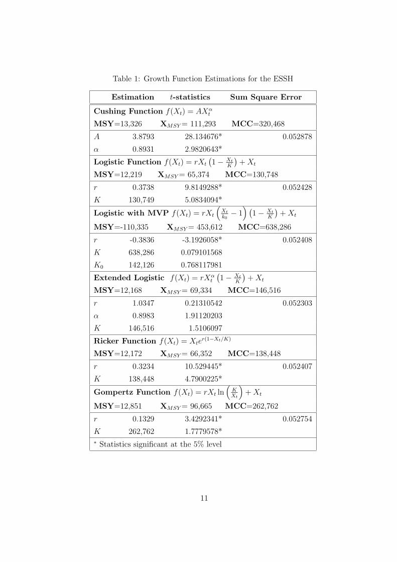
Table 1: Growth Function Estimations for the ESSH
Estimation t-statistics Sum Square Error
Cushing Function f(Xt) = AXαt
MSY=13,326 XMSY = 111,293 MCC=320,468
A 3.8793 28.134676* 0.052878
α 0.8931 2.9820643*
Logistic Function f(Xt) = rXt
(1− Xt
K
)+ Xt
MSY=12,219 XMSY = 65,374 MCC=130,748
r 0.3738 9.8149288* 0.052428
K 130,749 5.0834094*
Logistic with MVP f(Xt) = rXt
(Xt
k0− 1
) (1− Xt
K
)+ Xt
MSY=-110,335 XMSY = 453,612 MCC=638,286
r -0.3836 -3.1926058* 0.052408
K 638,286 0.079101568
K0 142,126 0.768117981
Extended Logistic f(Xt) = rXαt
(1− Xt
K
)+ Xt
MSY=12,168 XMSY = 69,334 MCC=146,516
r 1.0347 0.21310542 0.052303
α 0.8983 1.91120203
K 146,516 1.5106097
Ricker Function f(Xt) = Xter(1−Xt/K)
MSY=12,172 XMSY = 66,352 MCC=138,448
r 0.3234 10.529445* 0.052407
K 138,448 4.7900225*
Gompertz Function f(Xt) = rXt ln(
KXt
)+ Xt
MSY=12,851 XMSY = 96,665 MCC=262,762
r 0.1329 3.4292341* 0.052754
K 262,762 1.7779578*∗ Statistics significant at the 5% level
11
where r > 0 is the intrinsic growth rate and K represents environmental carrying capacity.
The results of this estimation imply r = 0.3234 and K = 138, 448. Both estimates are
significantly different from zero at the 5% level with t statistics of 10.5294 and 4.7900 for
r and K, respectively. With these estimations of the parameters r and K, the Maximum
Sustainable Yield (MSY) is 12, 172 tonnes, the biomass required for the MSY is 66, 352
tonnes and the Maximum Carrying Capacity (MCC) is 138, 448 tonnes.16 We can observe
that current stock, at about 27,074 tonnes in 2002, is far below that required to maintain
MSY. This supports the ICES prediction of current stock being outside safe biological limits
and the recommendation for zero captures in order to rebuild the stock.
Once these parameters are estimated, the stochastic process is calibrated in such a way
that the sequence of productivity shocks reproduces the stock and total catches observed
from 1982 to 2002. In order to do this, we take seven equidistant values for the state of the
productivity shock, that is
z ∈ {−0.0988,−0.0659,−0.0329, 0.0000, 0.0329, 0.0659, 0.0988} .
Given the information from the estimated errors, z and the values for the states of z, we
calculate the transition matrix, π, for the Markov chain that discretes a continuum process
in seven states following Tauchen (1986). The calibrated values are
tic and Gompertz functions fit the data well, but according to the Akaike criterium the Ricker
function was chosen because it presents the lowest sum of squared errors in the parameters
and the estimated biological aggregates are sensible. The P-test of Davidson and MacKinnon
(1981) was also calculated to select among the suitable functional forms. However the test
was inconclusive, probably due to the small sample size (21 observations).16The MSY is the maximum net growth of the biomass. In other words, the value of
the net growth for a stock level such that ∂ (F (Xt)−Xt) /∂Xt = 0. Recently, the National
Marine Fisheries Service of the USA has started to call this yield “long-term potential yield”.
The MCC is the maximum stock compatible with a null net growth of the resource, i.e. Xt
such that F (Xt) = 0.
12
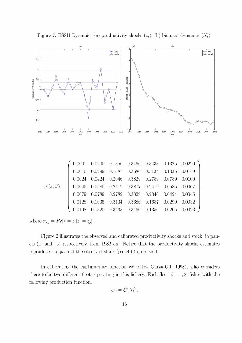
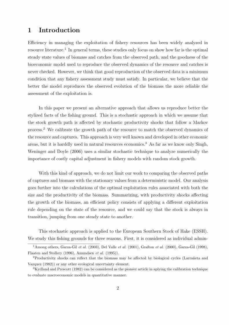
Figure 2: ESSH Dynamics (a) productivity shocks (zt); (b) biomass dynamics (Xt).
1982 1984 1986 1988 1990 1992 1994 1996 1998 2000 2002
−0.15
−0.1
−0.05
0
0.05
0.1
0.15
(a)
year
Pro
du
ctivity S
ho
cks
datamodel
1982 1984 1986 1988 1990 1992 1994 1996 1998 2000 20022
3
4
5
6
7
8
9x 10
4 (b)
year
Tota
l B
iom
ass (
Tonnes)
datamodel
π(z, z′) =
0.0001 0.0205 0.1356 0.3460 0.3433 0.1325 0.0220
0.0010 0.0299 0.1687 0.3686 0.3134 0.1035 0.0149
0.0024 0.0424 0.2046 0.3829 0.2789 0.0789 0.0100
0.0045 0.0585 0.2419 0.3877 0.2419 0.0585 0.0067
0.0079 0.0789 0.2789 0.3829 0.2046 0.0424 0.0045
0.0128 0.1035 0.3134 0.3686 0.1687 0.0299 0.0032
0.0198 0.1325 0.3433 0.3460 0.1356 0.0205 0.0023
,
where πi,j = Pr[z = zi|z′ = zj].
Figure 2 illustrates the observed and calibrated productivity shocks and stock, in pan-
els (a) and (b) respectively, from 1982 on. Notice that the productivity shocks estimates
reproduce the path of the observed stock (panel b) quite well.
In calibrating the capturability function we follow Garza-Gil (1998), who considers
there to be two different fleets operating in this fishery. Each fleet, i = 1, 2, fishes with the
following production function,
yi,t = ξθii,tX
λit ,
13
where ξi is the effort applied by fleet i and θi and λi are the elasticity of fleet i’s captures
with respect to effort and stock, respectively. The two fleets are heterogeneous in the sense
that the inputs behind the effort are different for the two fleets. In particular, effort is given
by
ξ1,t = dγ1
1,tTγ2t , (7)
ξ2,t = d2,t, (8)
where d and T represent days operating in the fishery and capacity of vessels, respectively.
Fleets 1 and 2 represent the trawler and the artisanal fleet, respectively. Parameters γ1
and γ2 represent the elasticity of the trawler fleet’s effort with respect to the number of
days fishing and the capacity of its vessels, respectively. Observe that with these production
functions and the sharing rule we can express effort in fishery 2 as a function of effort in
fishery 1,
p1 − w1ξ1,t
θ1y1,t(ξ1,t, Xt)= p2 − w2ξ2,t
θ2y2,t(ξ2,t, Xt), =⇒ ξ2 = ξ2(ξ1,t, Xt).
Table 2 indicates the capturability and market parameters used for our analysis. The
parameters comes from Garza-Gil (1998), where the reader will find how they are obtained
and their statistical properties. Note that the estimated parameters show that the larger the
stock is, the lower the share of the trawl fleet in total catches will be.17
4.2 Evaluation of the Management of the ESSH
Now we can investigate whether the observed exploitation paths for 1982-2002 in the ESSH
can be considered efficient given the initial conditions of the stock, X0 = X1982. To generate
the dynamic transition from the initial situation to the stochastic steady state we solve the
following dynamic programming,
V (z, X, Ymin, Ymax) = maxX′,ξ1,ξ2
2∑i=1
Πi(z,X,X ′, ξi) + βEz′ [V (z′, X ′, Ymin, Ymax)/z] ,
17It is easy to prove that the relative share of fleet i in total captures is given by (λi −λj)ξ
θ11 ξθ2
2 Xλ1+λ2−1, ∀i 6= j, which is negative provided λi < λj.
14
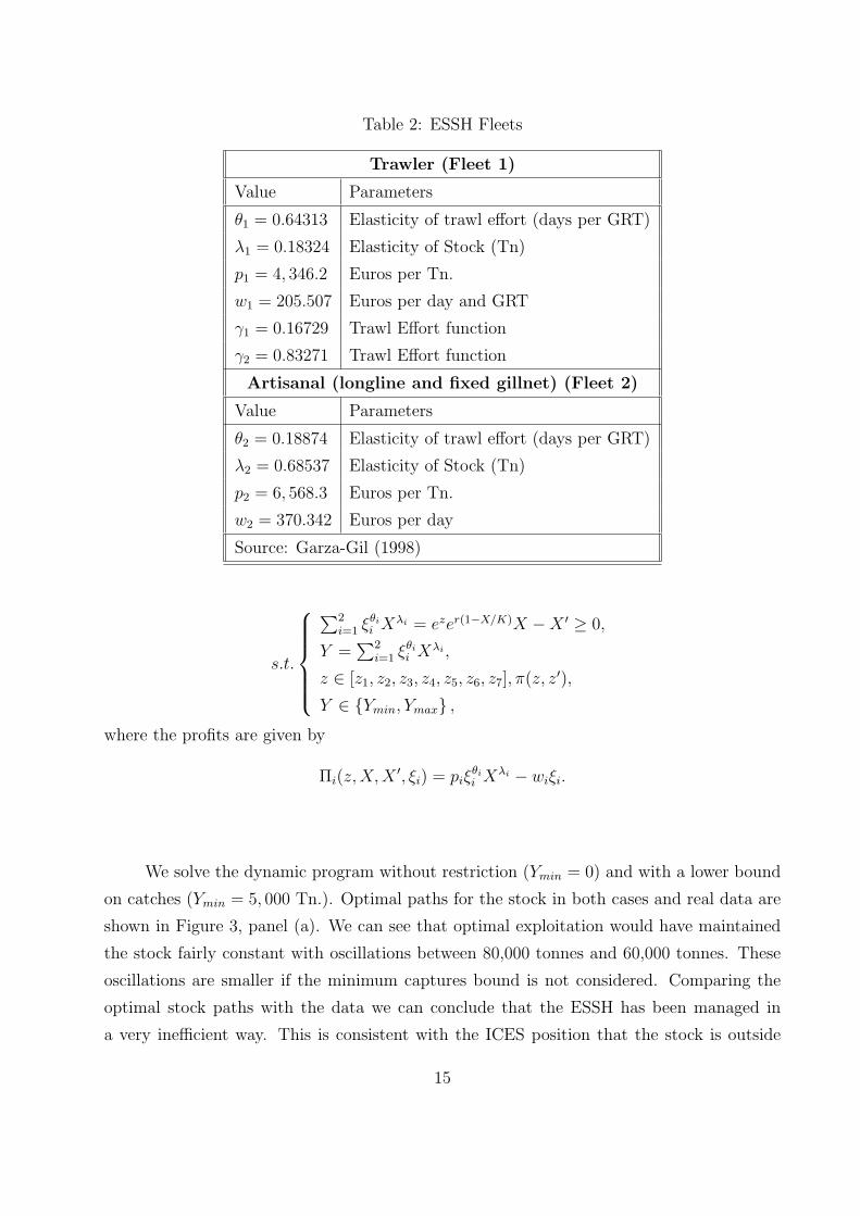
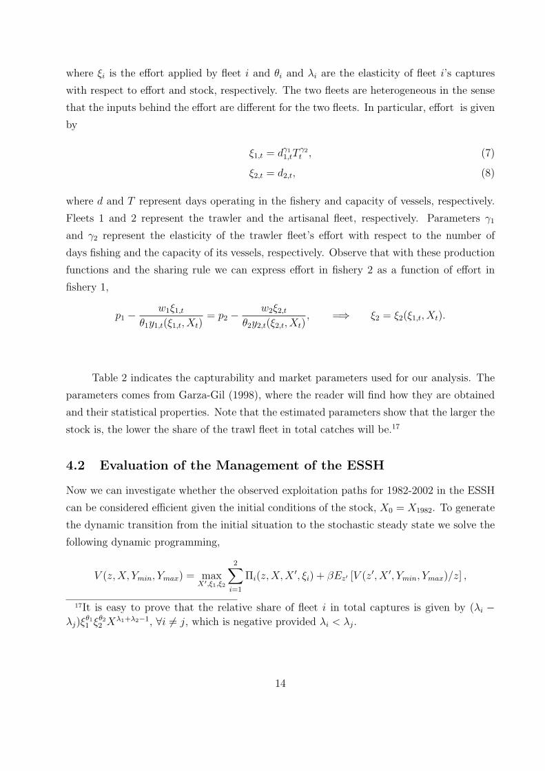
Table 2: ESSH Fleets
Trawler (Fleet 1)
Value Parameters
θ1 = 0.64313 Elasticity of trawl effort (days per GRT)
λ1 = 0.18324 Elasticity of Stock (Tn)
p1 = 4, 346.2 Euros per Tn.
w1 = 205.507 Euros per day and GRT
γ1 = 0.16729 Trawl Effort function
γ2 = 0.83271 Trawl Effort function
Artisanal (longline and fixed gillnet) (Fleet 2)
Value Parameters
θ2 = 0.18874 Elasticity of trawl effort (days per GRT)
λ2 = 0.68537 Elasticity of Stock (Tn)
p2 = 6, 568.3 Euros per Tn.
w2 = 370.342 Euros per day
Source: Garza-Gil (1998)
s.t.
∑2i=1 ξθi
i Xλi = ezer(1−X/K)X −X ′ ≥ 0,
Y =∑2
i=1 ξθii Xλi ,
z ∈ [z1, z2, z3, z4, z5, z6, z7], π(z, z′),
Y ∈ {Ymin, Ymax} ,
where the profits are given by
Πi(z, X, X ′, ξi) = piξθii Xλi − wiξi.
We solve the dynamic program without restriction (Ymin = 0) and with a lower bound
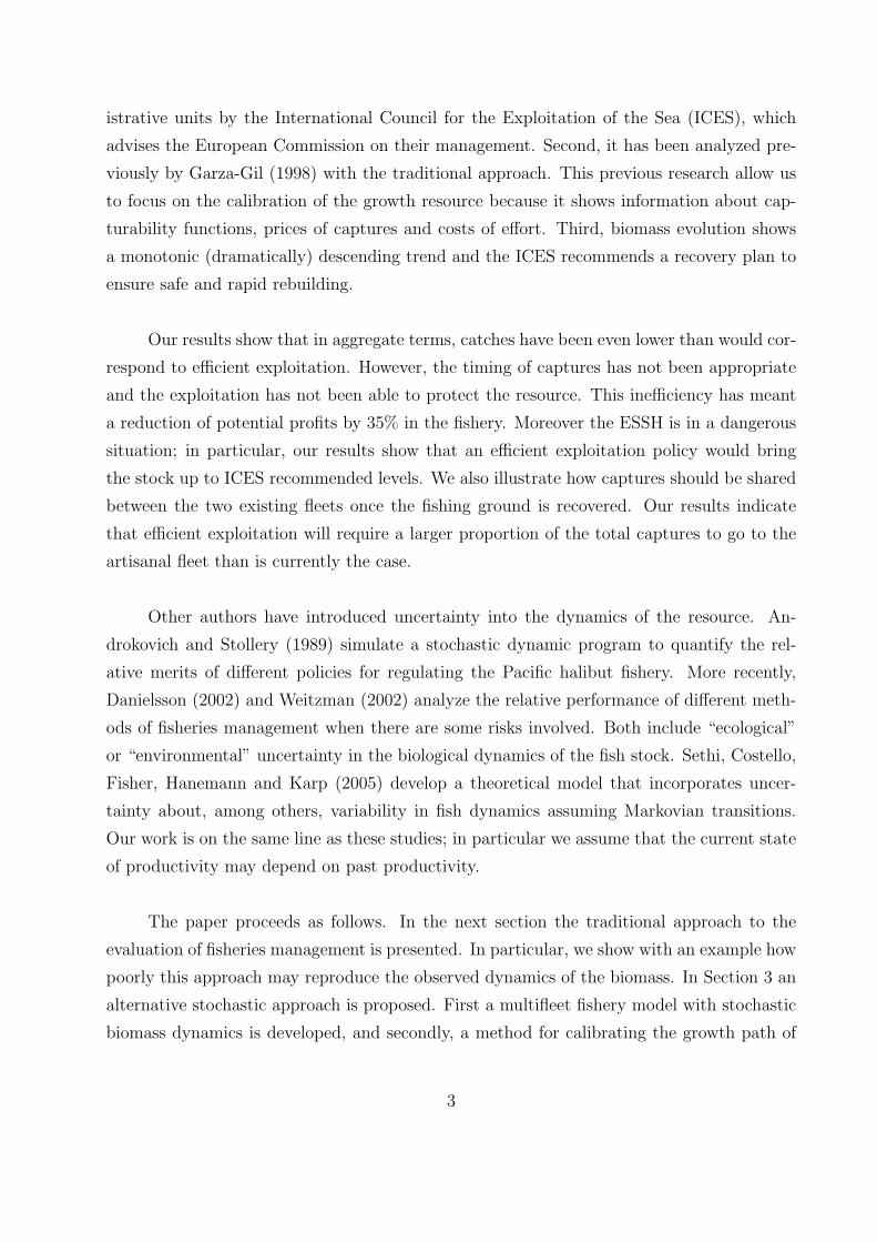
on catches (Ymin = 5, 000 Tn.). Optimal paths for the stock in both cases and real data are
shown in Figure 3, panel (a). We can see that optimal exploitation would have maintained
the stock fairly constant with oscillations between 80,000 tonnes and 60,000 tonnes. These
oscillations are smaller if the minimum captures bound is not considered. Comparing the
optimal stock paths with the data we can conclude that the ESSH has been managed in
a very inefficient way. This is consistent with the ICES position that the stock is outside
15
Figure 3: (a) Optimal Stock vs data; (b) Optimal Catches vs data with minimum catches of
5,000 Tn.
1982 1984 1986 1988 1990 1992 1994 1996 1998 2000 20022
3
4
5
6
7
8
9x 10
4
year
Tota
l B
iom
ass in T
n.
(a)
dataMinimum CatchOptimal
1982 1984 1986 1988 1990 1992 1994 1996 1998 2000 20020.4
0.6
0.8
1
1.2
1.4
1.6
1.8
2
2.2
2.4x 10
4
year
Tota
l C
atc
hes in T
n.
(b)
dataOptimal
safe biological limits and that it should be rebuilt. Since the optimal path associated with
a minimum catch of 5,000 Tn. is consistent with the current ICES objective, we decided to
use it as our benchmark for the rest of our simulations.
Figure 3, panel (b), illustrates the optimal evolution of captures in the benchmark
case and actual captures. Results show that until 1989 captures were greater than they
should have been for optimal exploitation. In particular, in 1983 captures were about 23,000
tonnes when optimal exploitation called for 16,000 tonnes. This excess of captures during
the 1980’s resulted in depletion of the stock. In 2002 biomass was about 27,000 Tn. while
optimal exploitation would have led to a resource stock of 60,000 Tn.
Figure 4 in panel (a) illustrates the path of aggregate profits associated with optimal
exploitation, with catch restrictions and with the observed data. Results show that optimal
exploitation would have implied low variability in aggregate profits over the period analyzed.
By contrast, observed profits dropped drastically in the fishery due to the overexploitation of
the stock in the early 1980s. In particular, we see that if the fleets had fished efficiently profit
in 2002 would have been almost 2.8 times the observed level. A similar pattern appears in
panel (b), where the effort of the artisanal fleet is shown. We see that the artisanal fleet
16

Figure 4: (a) Profits with minimum catches of 5,000 Tn , (b) Total Effort of Artisanal fleet
(days) vs data with minimum catches of 5,000 Tn.
1982 1984 1986 1988 1990 1992 1994 1996 1998 2000 20022
3
4
5
6
7
8
9
10
11
12x 10
7
year
Pro
fits
(a)
dataOptimal
1982 1984 1986 1988 1990 1992 1994 1996 1998 2000 20020
0.5
1
1.5
2
2.5
3
3.5x 10
4
year
Tota
l D
ays
(b)
dataOptimal
has reduced its effort enormously; however, optimal management of the fishery would have
enabled the initial level of effort to be maintained with no great variation.
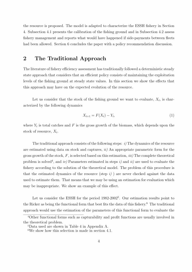
Figure 5 illustrates the efficient sharing of total catches between the two fleets. This
illustration is presented for two different levels of the resource stock: a low stock (20,000 Tn)
which represents a level close to current stock, and a high stock (60,000 Tn) which is close
to the optimal level. We observe several points. First, the larger the total captures are the
larger the share for the trawler fleet is (i.e. the capturability function is increasing). The
intuition for this result is clear. When captures are low the more efficient (artisanal) fleet
fishes most of them; however, as captures increase, the trawler fleet increases its catches by
a greater proportion because the artisanal fleet reaches its maximum capacity. Second, the
higher the resource stock is, the lower the participation of the trawler fleet in total captures
is. This is because an increase in stock implies more captures and, therefore, a more than
proportional increase in the captures of the less productive fleet (trawlers). And third, for
levels of stock and captures close to the optimal levels (i.e. stock close to 60,000 Tn and
captures about 12,000 Tn), the optimal sharing of catches implies that only the artisanal
fleet would operate in the fishery.
17
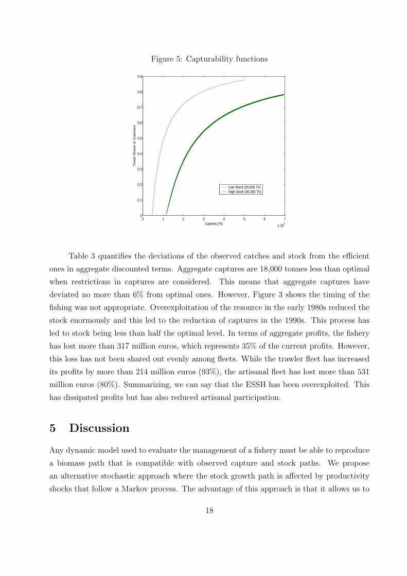
Figure 5: Capturability functions
0 1 2 3 4 5 6 7
x 104
0
0.1
0.2
0.3
0.4
0.5
0.6
0.7
0.8
0.9
Catches (Yt)
Tra
wl S
ha
re in
Ca
tch
es
Low Stock (20,000 Tn)High Stock (60,000 Tn)
Table 3 quantifies the deviations of the observed catches and stock from the efficient
ones in aggregate discounted terms. Aggregate captures are 18,000 tonnes less than optimal
when restrictions in captures are considered. This means that aggregate captures have
deviated no more than 6% from optimal ones. However, Figure 3 shows the timing of the
fishing was not appropriate. Overexploitation of the resource in the early 1980s reduced the
stock enormously and this led to the reduction of captures in the 1990s. This process has
led to stock being less than half the optimal level. In terms of aggregate profits, the fishery
has lost more than 317 million euros, which represents 35% of the current profits. However,
this loss has not been shared out evenly among fleets. While the trawler fleet has increased
its profits by more than 214 million euros (93%), the artisanal fleet has lost more than 531
million euros (80%). Summarizing, we can say that the ESSH has been overexploited. This
has dissipated profits but has also reduced artisanal participation.
5 Discussion
Any dynamic model used to evaluate the management of a fishery must be able to reproduce
a biomass path that is compatible with observed capture and stock paths. We propose
an alternative stochastic approach where the stock growth path is affected by productivity
shocks that follow a Markov process. The advantage of this approach is that it allows us to
18
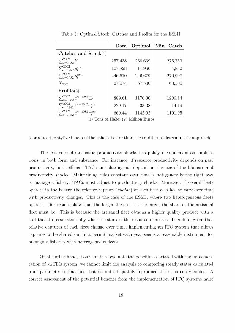
Table 3: Optimal Stock, Catches and Profits for the ESSH
Data Optimal Min. Catch
Catches and Stock(1)∑2002t=1982 Yt 257,438 258,639 275,759∑2002t=1982 ytrw.
t 107,828 11,960 4,852∑2002t=1982 yart.
t 246,610 246,679 270,907
X2001 27,074 67,500 60,500
Profits(2)∑2002t=1982 βt−1982Πt 889.61 1176.30 1206.14∑2002t=1982 βt−1982πtrw.
t 229.17 33.38 14.19∑2002t=1982 βt−1982πart.
t 660.44 1142.92 1191.95
(1) Tons of Hake; (2) Million Euros
reproduce the stylized facts of the fishery better than the traditional deterministic approach.
The existence of stochastic productivity shocks has policy recommendation implica-
tions, in both form and substance. For instance, if resource productivity depends on past
productivity, both efficient TACs and sharing out depend on the size of the biomass and
productivity shocks. Maintaining rules constant over time is not generally the right way
to manage a fishery. TACs must adjust to productivity shocks. Moreover, if several fleets
operate in the fishery the relative capture (quotas) of each fleet also has to vary over time
with productivity changes. This is the case of the ESSH, where two heterogeneous fleets
operate. Our results show that the larger the stock is the larger the share of the artisanal
fleet must be. This is because the artisanal fleet obtains a higher quality product with a
cost that drops substantially when the stock of the resource increases. Therefore, given that
relative captures of each fleet change over time, implementing an ITQ system that allows
captures to be shared out in a permit market each year seems a reasonable instrument for
managing fisheries with heterogeneous fleets.
On the other hand, if our aim is to evaluate the benefits associated with the implemen-
tation of an ITQ system, we cannot limit the analysis to comparing steady states calculated
from parameter estimations that do not adequately reproduce the resource dynamics. A
correct assessment of the potential benefits from the implementation of ITQ systems must
19

consider quotas as variables that depend on the size and productivity of the biomass because
the participation of each fleet depends on relative productivity. In the case of the ESSH the
artisanal fleet, whose productivity increases with the stock, would buy all the permits in the
auction as long as the stock reaches the efficient value. At the same time, the participation
of the trawler fleet would drop from the current level to zero.
20
References
[1] Amundsen, E. S., T Bjørndal and J. M. Conrad, 1995, Open Access Harvesting on the
Northeast Atlantic Minke Whale, Environmental and Resource Economics 6, 167-185.
[2] Androkovich, R.A. and K.R. Stollery, 1989, Regulation of Stochastic Fisheries: A Com-
parison of Alternative Methods in the Pacific Halibut Fishery, Marine Resource Eco-
nomics 6, 109-22.
[3] Danielsson, A., 2002, Efficiency of Catch and Effort Quotas in the Presence of Risk,
Journal of Environmental Economics and Management 43, 20-33.
[4] Davidson, R. and J.G. MacKinnon, 1981, Several test for model specification in the
presence of alternative hypothesis, Econometrica 49, 781-793.
[5] Del Valle, I., I. Astorkiza and K. Astorkiza, 2001, Is the Current Regulation of the
VIII Division European Anchovy Optimal?, Environmental and Resource Economics
19, 53-72.
[6] Flaaten, O. and K. Stollery, 1996, The Economic Costs of Biological Predation, Envi-
ronmental and Resource Economics 8, 75-95.
[7] Garza-Gil, M.D., 1998, ITQ Systems in Multifleet Fisheries. An Application for Iberoat-
lantic Hake, Environmental and Resource Economics 11, 79-92.
[8] Garza-Gil, M.D., M.M. Varela-Lafuente and J.C. Surs-Regueiro, 2003, European Hake
Fishery Biobeconomic Management (Southern Stock) Applying and Effort Tax, Fish-
eries Research 60, 199-206.
[9] Grafton, R.Q., L.K. Sandal and S.I. Steinshamn, 2000, How to IMprove the Managmenet
of Renewable Resources: The Case of the Canada’s Northern Cod Fishery, American
Journal of Agricultural Economics 82, 570-580.
[10] ICES, 2003. Annual Report of the ICES Advisory Committee on fishery Managment.
Cooperative Research Report No 261.
[11] ICES CM 2004/ACFM:02. Report elaborated by the Working Group on the Assessment
of Southern Stock of Hake, Monk and Megrim.
[12] Kydland, F.E. and E.C. Prescott, 1982, Time to Build and Aggregate Fluctuations,
Econometrica 50, 1345-70.
21
[13] Larraeta, M.G. and A. Vazquez, 1982, On a Possible Meaning of the Polar Motion in
the Ecology of North Atlantic Cod (Gadus Morhua), ICES CM 1982/G:14.
[14] Meade, N. and T. Islam, 1995, Forcasting with Growth Curves: An Empirical Compar-
ison, International Journal of Forecasting 11, 199-215.
[15] Sethi, G., C. Costello, A. Fisher, M. Hanemann and L. Karp, 2005, Fishery Managment
under Multiple Uncertainty, Journal of Environmental Economics and Management
50/2, 300-18.
[16] Singh, R., Q. Weninger and M. Doyle, 2006, Fisheries Managment with Stock Growth
Uncertainty and Costly Capital Adjustment, Journal of Environmental Economics and
Management 52/2, 582-99.
[17] STECF, 2004. Review of Scientific Advice for 2004. Commission Staff Working Paper,
SEC(2004) 372.
[18] Tauchen, G., 1986, Finite State Markov-Chain Approximations to Univariate and Vector
Autoregresions, Economic Letters 20, 177-81.
[19] Weitzman, M.L., 2002, Landing Fees vs Harvest Quotas with Uncertain Fish Stocks,
Journal of Environmental Economics and Management 43, 325-38.
22
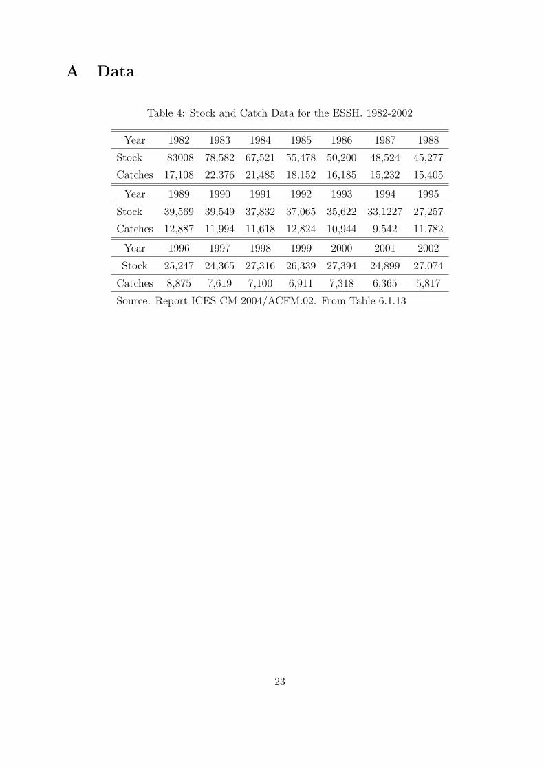
A Data
Table 4: Stock and Catch Data for the ESSH. 1982-2002
Year 1982 1983 1984 1985 1986 1987 1988
Stock 83008 78,582 67,521 55,478 50,200 48,524 45,277
Catches 17,108 22,376 21,485 18,152 16,185 15,232 15,405
Year 1989 1990 1991 1992 1993 1994 1995
Stock 39,569 39,549 37,832 37,065 35,622 33,1227 27,257
Catches 12,887 11,994 11,618 12,824 10,944 9,542 11,782
Year 1996 1997 1998 1999 2000 2001 2002
Stock 25,247 24,365 27,316 26,339 27,394 24,899 27,074
Catches 8,875 7,619 7,100 6,911 7,318 6,365 5,817
Source: Report ICES CM 2004/ACFM:02. From Table 6.1.13
23
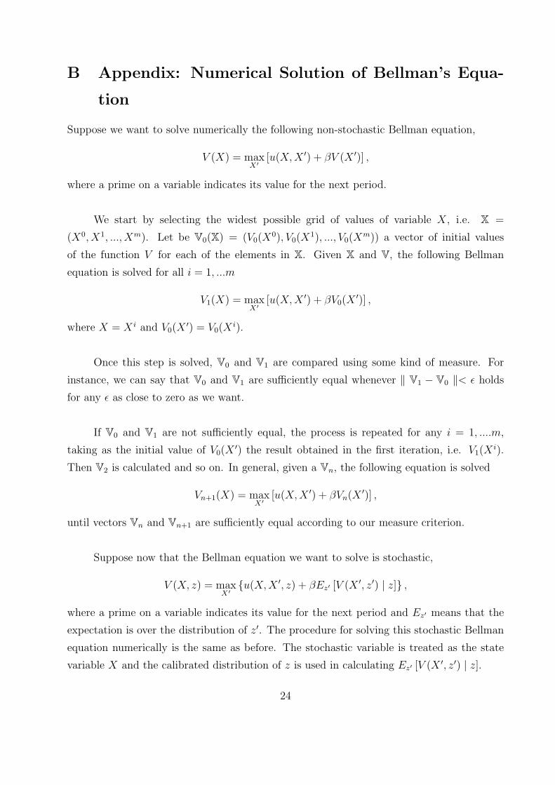
B Appendix: Numerical Solution of Bellman’s Equa-
tion
Suppose we want to solve numerically the following non-stochastic Bellman equation,
V (X) = maxX′
[u(X, X ′) + βV (X ′)] ,
where a prime on a variable indicates its value for the next period.
We start by selecting the widest possible grid of values of variable X, i.e. X =
(X0, X1, ..., Xm). Let be V0(X) = (V0(X0), V0(X
1), ..., V0(Xm)) a vector of initial values
of the function V for each of the elements in X. Given X and V, the following Bellman
equation is solved for all i = 1, ...m
V1(X) = maxX′
[u(X, X ′) + βV0(X′)] ,
where X = X i and V0(X′) = V0(X
i).
Once this step is solved, V0 and V1 are compared using some kind of measure. For
instance, we can say that V0 and V1 are sufficiently equal whenever ‖ V1 − V0 ‖< ε holds
for any ε as close to zero as we want.
If V0 and V1 are not sufficiently equal, the process is repeated for any i = 1, ....m,
taking as the initial value of V0(X′) the result obtained in the first iteration, i.e. V1(X
i).
Then V2 is calculated and so on. In general, given a Vn, the following equation is solved
Vn+1(X) = maxX′
[u(X, X ′) + βVn(X ′)] ,
until vectors Vn and Vn+1 are sufficiently equal according to our measure criterion.
Suppose now that the Bellman equation we want to solve is stochastic,
V (X, z) = maxX′
{u(X,X ′, z) + βEz′ [V (X ′, z′) | z]} ,
where a prime on a variable indicates its value for the next period and Ez′ means that the
expectation is over the distribution of z′. The procedure for solving this stochastic Bellman
equation numerically is the same as before. The stochastic variable is treated as the state
variable X and the calibrated distribution of z is used in calculating Ez′ [V (X ′, z′) | z].
24