The Estimation of Nominal and Real Yield

Curves from Government

Bonds in Israel

Zvi Wiener and Helena Pompushko

2006.03 June 2006

2

The Estimation of Nominal and Real Yield

Curves from Government

Bonds in Israel

Zvi Wiener and Helena Pompushko

2006.03 June 2006

The views expressed in this paper are those of the authors only, and do not necessarily

represent those of the Bank of Israel.

Email: mswiener@mscc.huji.ac.il

helenap@boi.gov.il

© Bank of Israel

Passages may be cited provided source is specified

Catalogue no. 3111506003/5

Monetary Department, Bank of Israel, POB 780, Jerusalem 91007

http://www.bankisrael.gov.il

3

The Estimation of Nominal and Real Yield

Curves from Government Bonds in Israel

Zvi Wiener1 and Helena Pompushko2

Acknowledgements. The project was carried out in the Monetary Department of the Bank of Israel. The authors wish to thank members of the Monetary Department of the Bank of Israel for the data and useful comments. Zvi Wiener acknowledges partial funding of his research from the Krueger Center for Finance and Banking of the School of Business Administration, The Hebrew University, Jerusalem and the Monetary Department of the Bank of Israel.

1 School of Business Administration, The Hebrew University of Jerusalem, Israel 2 Monetary Department, Bank of Israel

4

The estimation of nominal and real yield curves

from government bonds in Israel

Abstract We develop and test a mathematical method of deriving zero yield curve from market

prices of government bonds. The method is based on a forward curve approximated

by a linear (or piecewise constant) spline and should be applicable even for markets

with low liquidity. The best fitting curve is derived by minimizing the penalty

function. The penalty is defined as a sum of squared price discrepancies (theoretical

curve based price minus market closing price) weighted by trade volume and an

additional penalty for non-smoothness of the yield curve. The algorithm is applied to

both nominal and CPI linked bonds traded in Israel (some segments of these markets

have low liquidity). The resulting two yield curves can be used for derivation of

market expected inflation rate. The main problems are low liquidity of some bonds

and imperfect linkage to inflation in the CPI linked market. Use of forward curves as

the state space for the minimization problem leads to a stable solution that fits the data

very well and can be used for calculating forward rates.

5

תקציר

ממחירי) קופון ללא (אפס ריביות עקום לגזירת נומרית שיטה ובוחנים מפתחים אנו, זה במאמר

הזה הריבית עקום. רציף בחישוב פורוורד ריבית עקום על מבוססת השיטה. חוב אגרות של השוק

עקום. נמוכה הנזילות רמת שבהם בשווקים גם ליישום ניתנת הזו והשיטה spline בשיטת נבנה

משני בנויה הקנס פונקציית. הקנס פונקציית של המינימום נקודת מציאת ידי על נבנה הריביות

) אפס עקום על המבוסס (התיאורטי המחיר בין התאמה חוסר מייצג הראשון החלק. חלקים

את מייצג השני החלק. סדרה כל של הנזילות רמת את המשקפות משקולות עם, שוק ומחירי

.הריביות עקום של החלקות חוסר

והן המדד צמודת השקלית הריבית בעקום הן הישראלי בשוק האלגוריתם את מיישמים אנו

המאפשרות ריבית עקומות שתי היא האלגוריתם תוצאת. הנומינלית השקלית הריבית בעקום

רמת הן מתמודדים אנו איתן המרכזיות הבעיות. העתידית האינפלציה לגבי השוק ציפיות גזירת

. מדד צמודות ח"באג מלאה לא והצמדה השוק של בחלקים כהנמו נזילות

התאמה עם יציב לפתרון מוביל האופטימיזציה בבעיית כנעלם העתידי הריביות בעקום השימוש

. forward-ו spot ריביות של רציפה גזירה מאפשר גם הוא. שוק נתוני מול טובה

6

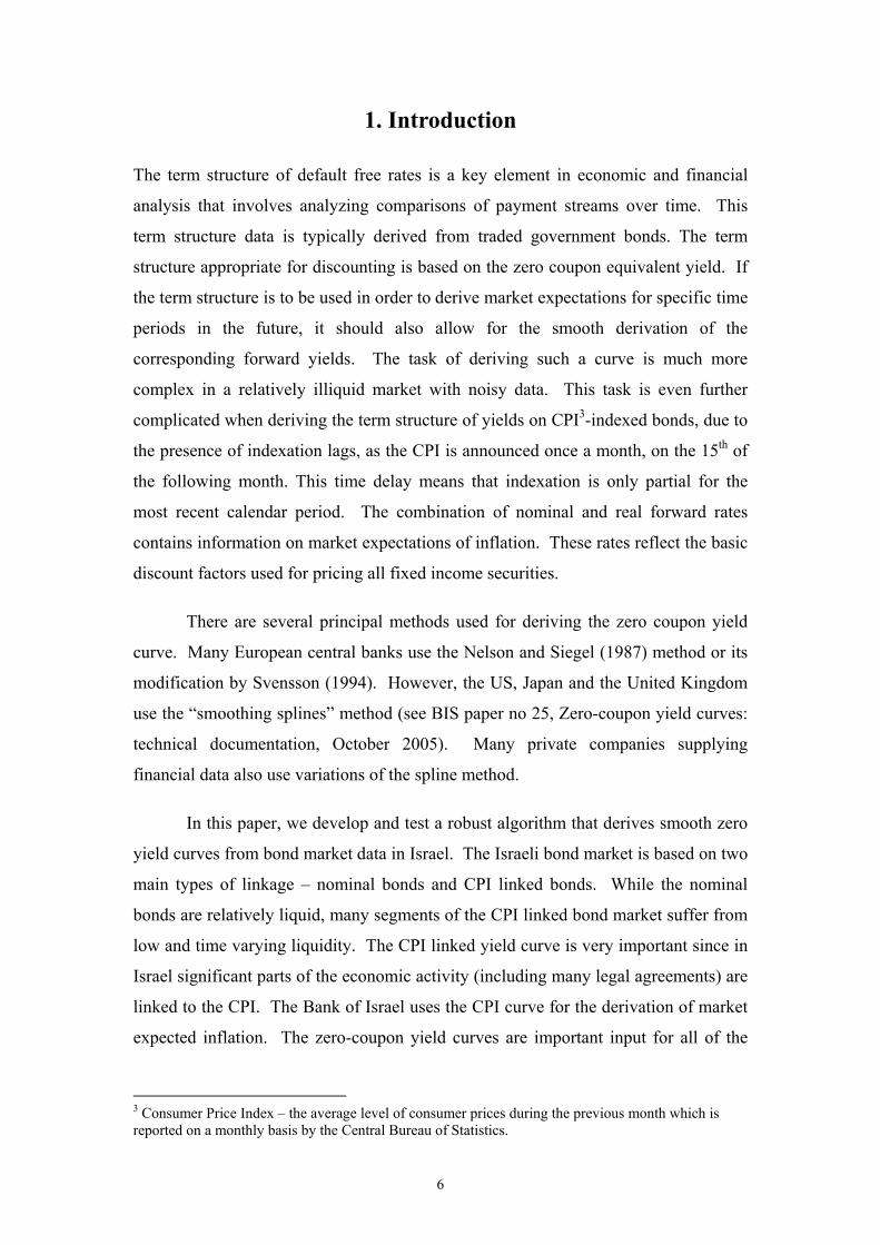
1. Introduction

The term structure of default free rates is a key element in economic and financial

analysis that involves analyzing comparisons of payment streams over time. This

term structure data is typically derived from traded government bonds. The term

structure appropriate for discounting is based on the zero coupon equivalent yield. If

the term structure is to be used in order to derive market expectations for specific time

periods in the future, it should also allow for the smooth derivation of the

corresponding forward yields. The task of deriving such a curve is much more

complex in a relatively illiquid market with noisy data. This task is even further

complicated when deriving the term structure of yields on CPI3-indexed bonds, due to

the presence of indexation lags, as the CPI is announced once a month, on the 15th of

the following month. This time delay means that indexation is only partial for the

most recent calendar period. The combination of nominal and real forward rates

contains information on market expectations of inflation. These rates reflect the basic

discount factors used for pricing all fixed income securities.

There are several principal methods used for deriving the zero coupon yield

curve. Many European central banks use the Nelson and Siegel (1987) method or its

modification by Svensson (1994). However, the US, Japan and the United Kingdom

use the “smoothing splines” method (see BIS paper no 25, Zero-coupon yield curves:

technical documentation, October 2005). Many private companies supplying

financial data also use variations of the spline method.

In this paper, we develop and test a robust algorithm that derives smooth zero

yield curves from bond market data in Israel. The Israeli bond market is based on two

main types of linkage – nominal bonds and CPI linked bonds. While the nominal

bonds are relatively liquid, many segments of the CPI linked bond market suffer from

low and time varying liquidity. The CPI linked yield curve is very important since in

Israel significant parts of the economic activity (including many legal agreements) are

linked to the CPI. The Bank of Israel uses the CPI curve for the derivation of market

expected inflation. The zero-coupon yield curves are important input for all of the

3 Consumer Price Index – the average level of consumer prices during the previous month which is reported on a monthly basis by the Central Bureau of Statistics.

7

above. The method described below calculates these curves in a smooth and robust

manner.

By smooth we mean that one can derive forward rates from the same curve

and get reasonable results, even if the market is not very liquid (infrequent trades, low

volume and slow adjustment of prices). By robust we mean an algorithm that does

not suddenly change shape from one day to another due to technical reasons. We also

expect the shape of the yield curve to be stable, relative to the input data set. For

example, when dropping one bond with a small volume of trade we should not expect

a significant change in the whole term structure.

The advantage of using the zero-coupon yield curve is that it allows an

immediate discount of every single future payment. The alternative that is often used

is based on yield to maturity. This yield can be calculated much more easily, but its

use is very limited, as it is appropriate only for a given schedule of payments and can

not be used for any other cashflow, (which differs either in the coupon amounts or in

timing). Thus, the yield to maturity of a coupon bond is not a good measure of the

time value of money and it should be stripped before it is used for discounting. The

derivation of forward rates is a mathematical procedure that requires taking the

derivative of the term structure with respect to the time to maturity. Thus any non-

smooth yield curve will lead to artificial jumps in the forward rates and consequently

to incorrect conclusions regarding market expectations.

The liquidity of the Israeli government bond market is low in some segments

(short term CPI linked bonds for example). Thus the market data is often noisy and

can not be used without taking this into account.

We describe below an algorithm that overcomes these difficulties as it

searches for the best fitted yield curve based on forward splines, where the fitting

penalty takes into account the liquidity of each issue. Moreover, for the CPI linked

bonds we break up the holding period into CPI linked and unlinked periods and

discount each cashflow appropriately.

8

2. Government bonds in Israel

The Israeli government bond market has (at the end of 2005) a market capitalization

of 262B NIS4 with an average daily trade volume in 2005 of about 1.1B NIS. In

comparison, the stock market in Israel has a market value of about 506B NIS with an

average daily trade volume of 965M NIS, the corporate bond market has a value of

105B NIS with an average daily trade volume of about 250M NIS. Most institutional

investors rely on the government bonds as the core of their portfolios. There are 4

main types of government bonds issued in the local market. They are named Makam,

Shahar, Gilon, and Galil. The table below summarizes their main characteristics. The

shekel dollar exchange rate in 2005 was around the level of 4.5 NIS = 1 USD.

Name Original

maturity

Linkage Coupon Outstanding

notional

Average

daily trade

volume

Makam Up to 1

year

Nominal Zero coupon NIS 71 B NIS 585 M

Shahar 2-15 years nominal Fixed, annual NIS 89 B NIS 559 M

Gilon 2-10 years nominal Floating, annual NIS 57 B NIS 163 M

Galil 7-20 years CPI-

linked

Fixed, annual NIS 114 B NIS 351 M

4 NIS stands for New Israeli Shekel which is the name of the Israeli currency, also referred to as the shekel.

9

3. Methods of calculating zero-coupon yield curves

There are three types of methods used for the estimation of a zero-coupon yield curve

from bond market data. The first one is based on an assumption of a parametric form

of a yield curve. The most popular version of this method was developed by Nelson

and Siegel (1987). This method assumes that the instantaneous forward rates take the

following functional form:

τ

τβββ

tNS ettf

−⋅

++= 210)(

Here β0, β1, and τ are parameters that determine the shape of the term structure.

Although this functional form allows for several different shapes of the term structure,

Svensson (1994) suggested a richer family with an additional term (and two more

parameters).

21

23

1210)( ττ

τβ

τβββ

ttSv etettf

−−

⋅+⋅

++=

This form allows for two humps and it includes the Nelson Siegel model as a special

case (when β3=0). The problem with the parametric methods like these is that the

functional form assumed from mathematical convenience does not reflect the

economic behavior of interest rates. Another problem is that a small change in a price

of a long term bond can lead to a change of the short end of the derived zero-coupon

yield curve for purely technical reasons. The third problem is that often the shape of

the yield curve based on a parametric model is not robust and changes significantly

after a relatively small change in prices.

The second method is based on bootstrapping and can be used for a very

efficient market only, where prices are observed simultaneously; there is a variety of

liquid bonds with different maturities covering the whole range of time. This method

is not appropriate for a smaller market with few bonds, suffering from low liquidity.

The third method is based on splines (functions defined piecewise). This

method was developed in Vasicek and Fong (1982), and Fisher, Nychka, and Zervos

(1995). It is based either on a fixed or variable grid and an optimization procedure

that minimizes some penalty functions.

The goal of this paper is to construct a robust algorithm for calculating the

term structure of interest rates from market prices of traded government bonds. The

10

term structure we are looking for is a zero-coupon term structure that can be directly

used for discount factor. Moreover, we would like to have as a result a smooth term

structure. The trade off between better matching market prices, robustness and

smoothness will be described below. The algorithm is implemented for both nominal

and CPI linked sectors.

We use a fixed time grid, and interpolate forward rates between grid nodes

using a simple linear function.5 Then, for any given set of key forward rates one can

calculate the theoretical prices and the degree of non-smoothness of the resulting

curve. The minimization of these two penalties (with some weights) leads to the zero-

coupon term structure of interest rates.

4. Data

The input of the model is based on the (almost) fixed data base of future cashflows

that are reflected in the market price, the daily closing prices of government bonds,

the volume of trade, and the anticipated inflation for the period between the last CPI

report and the input date.

Due to low liquidity occasionally there are very noisy observations. We apply

a filter that excludes any suspicious data, such as bonds that have negative yields, low

trade volume, or very unusual price changes.

In order to identify unusual price changes, we analyze the history of each bond

over 45-60 days, and calculate the canonical correlations of the past with the current

change. This method uses the STATESPACE procedure of SAS and represents a

stationary multivariate time series X(t) of dimensions R in the following form:

)()1()( tEGtZFtZ ⋅+−⋅= (AIC - Akaike's information criterion)

Where Z(t) is the vector process of dimension S=R+1. The first R components of Z(t)

are in fact X(t) and the last component is the prediction of X(t+1) based on the

history. F is an S-by-S transition matrix, and G is an S-by-R matrix calculated by

SAS. E(t) is an R-dimensional noise independent of X(t).

The procedure fits a sequence of vector autoregressive models using Yule-Walker

equations and selects the order for which Akaike's Information Criterion (AIC) is

minimized (0.0001). After using this procedure, we have a residual for each price of

5 The same method will work for other types of interpolation between nodes.

11

each bond. We calculate the average residual for this date over all bonds and compute

the ratio of the actual residual of a bond to the average of all bonds on the same date.

If the ratio is greater than 3, we ignore this observation.

Typically the daily set consists of 10-12 bills (Makam), 6-8 notes (Shahar),

and 8-34 CPI-linked securities (Galil). The nominal bonds are almost always liquid,

while CPI-linked bonds are less liquid, especially those with a time to maturity of up

to two years. The CPI –linked bonds also have big price fluctuations (probably also

due to illiquidity).

5. Description of the algorithm for the nominal yield curve

For the nominal yield curve we use the following time grid:

(T1, T2, …, TN) = (0, 3M, 6M, 9M, 1Y, 2Y, 3Y, 5Y, 7Y, 10Y). Define the yet

unknown vector of forward rates by (F1, F2, …, FN). Interpolate the forward rate

linearly between the grid nodes by using linear interpolation. For Ti<t<Ti+1 we have

(1) 111

1)( +++

+

−−

+−−

= iii

ii

ii

i FTT

TtFTTtTtf

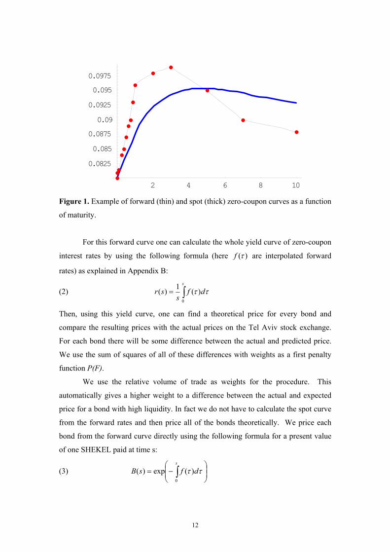
An example of a graph showing piecewise linear interpolation between the nodes of

the fixed grid is provided below, in figure 1. This graph is based on the following

forward rates:

F=(3.58%,3.84%,4.09%,4.32%,4.54%,5.53%,6.67%,8.82%,8.91%,6.82%).

The forward rates are shown as represented by the (red) dots connected by the thin

line and the spot curve is represented by the smoother, thicker (blue) line. The graph

demonstrates the way that the spot curve is smooth, even when the curve of the

forward rates is not.

12

2 4 6 8 10

0.08250.0850.08750.09

0.09250.0950.0975

Figure 1. Example of forward (thin) and spot (thick) zero-coupon curves as a function

of maturity.

For this forward curve one can calculate the whole yield curve of zero-coupon

interest rates by using the following formula (here )(τf are interpolated forward

rates) as explained in Appendix B:

(2) ∫=s

dfs

sr0

)(1)( ττ

Then, using this yield curve, one can find a theoretical price for every bond and

compare the resulting prices with the actual prices on the Tel Aviv stock exchange.

For each bond there will be some difference between the actual and predicted price.

We use the sum of squares of all of these differences with weights as a first penalty

function P(F).

We use the relative volume of trade as weights for the procedure. This

automatically gives a higher weight to a difference between the actual and expected

price for a bond with high liquidity. In fact we do not have to calculate the spot curve

from the forward rates and then price all of the bonds theoretically. We price each

bond from the forward curve directly using the following formula for a present value

of one SHEKEL paid at time s:

(3)

−= ∫

s

dfsB0

)(exp)( ττ

13

By working with fixed coupons, we can immediately price each traded bond by

summing up its discounted cash flow. The total penalty of the first type is defined as:

(4) ( )∑ −=bonds

iii pricemarketFprice

volumetradetotalvolumetrade

FP 2)()(

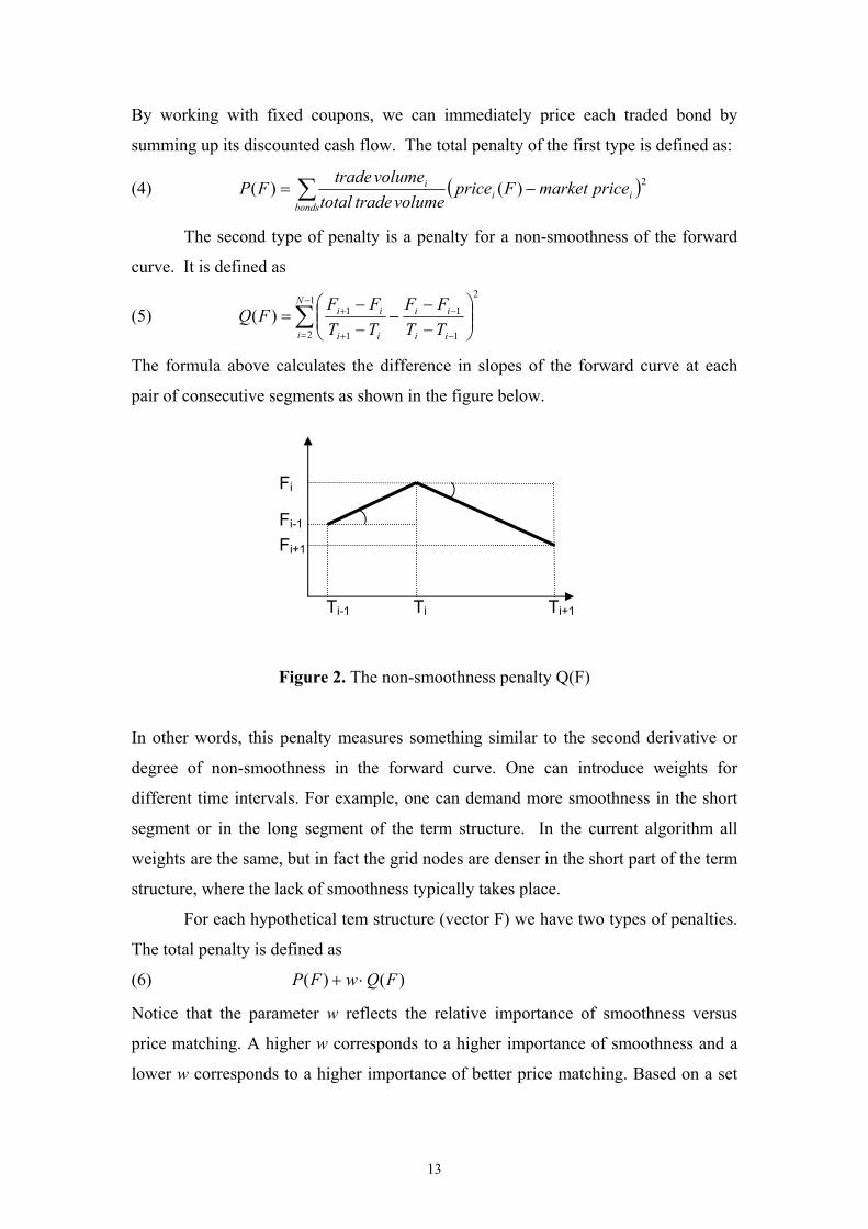
The second type of penalty is a penalty for a non-smoothness of the forward

curve. It is defined as

(5) ∑−

= −

−

+

+

−−

−−−

=1

2

2

1

1

1

1)(N

i ii

ii

ii

ii

TTFF

TTFF

FQ

The formula above calculates the difference in slopes of the forward curve at each

pair of consecutive segments as shown in the figure below.

Figure 2. The non-smoothness penalty Q(F)

In other words, this penalty measures something similar to the second derivative or

degree of non-smoothness in the forward curve. One can introduce weights for

different time intervals. For example, one can demand more smoothness in the short

segment or in the long segment of the term structure. In the current algorithm all

weights are the same, but in fact the grid nodes are denser in the short part of the term

structure, where the lack of smoothness typically takes place.

For each hypothetical tem structure (vector F) we have two types of penalties.

The total penalty is defined as

(6) )()( FQwFP ⋅+

Notice that the parameter w reflects the relative importance of smoothness versus

price matching. A higher w corresponds to a higher importance of smoothness and a

lower w corresponds to a higher importance of better price matching. Based on a set

Ti-1 Ti Ti+1

Fi-1

Fi+1

Fi

14

of experiments we have chosen the value of w to be equal 1, as this leads to a good

balance of price matching and smoothness.

Now we perform a multidimensional optimization procedure in which we

search for an “optimal” term structure that matches the two criteria simultaneously by

minimizing the expression (6) over all admissible forward yield curves. A result of

this minimization is a forward rate vector F. As soon as the optimal forward curve is

found, one can calculate the spot curve, using (2). This gives the resulting nominal

zero-coupon yield curve.

We observed several cases in which the optimization procedure is not well

defined due to a high ratio of the biggest and the smallest eigenvalue of the matrix of

second derivatives. In such a case we recommend using the conjugate gradient

instead of the method of steepest descent (the gradient method).

6. CPI linked bonds

The CPI linked government bonds provide only an approximate indexation due to the

fact that the CPI index is measured discretely with a time delay. In fact the “known

index” is used each time that a payment occurs. This index is the one that was

measured on most recent 15-th day of a month and it reflects the average price level

during the month that ended 15 days earlier. For example, if a payment takes place on

May 31, the index that was announced on May 15 will be used. This index

corresponds to the average price level during the month of April. This creates a delay

of approximately a month and a half.

A similar situation exists when we need to price a linked bond on, say May 10.

Then the last reported index was announced on April 15 and it corresponds to the

average price level of March. This can create a delay of up to two months.

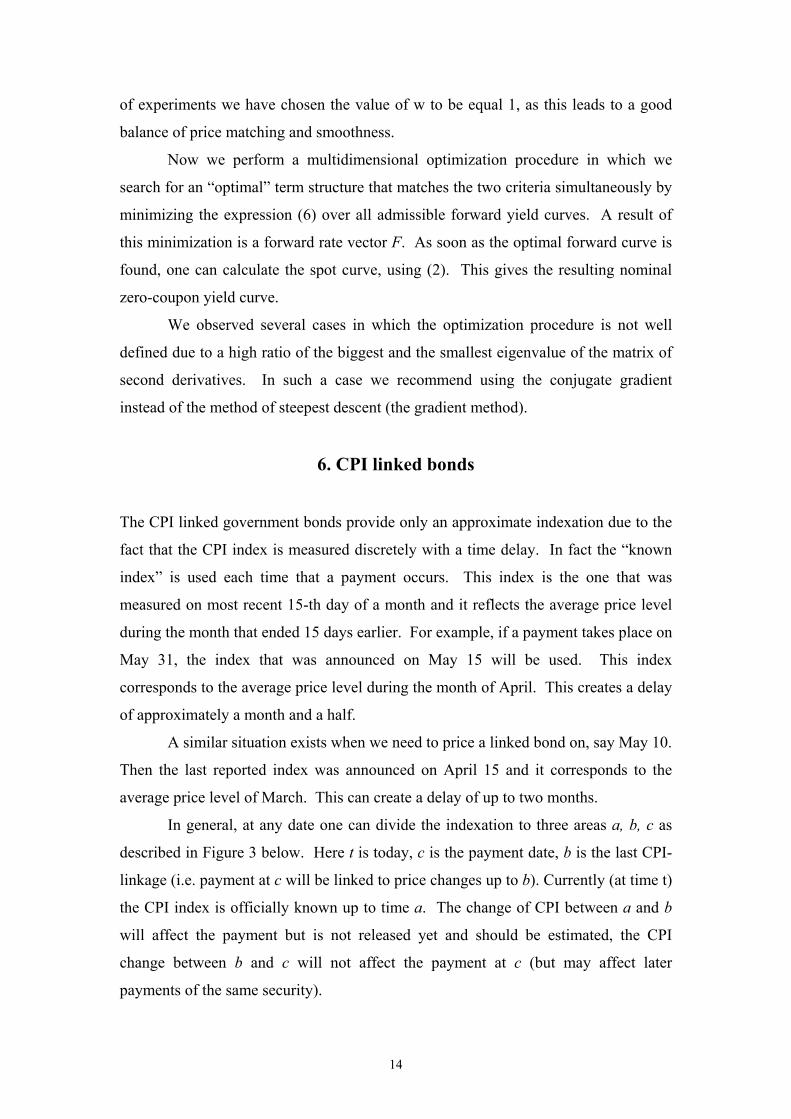
In general, at any date one can divide the indexation to three areas a, b, c as

described in Figure 3 below. Here t is today, c is the payment date, b is the last CPI-

linkage (i.e. payment at c will be linked to price changes up to b). Currently (at time t)

the CPI index is officially known up to time a. The change of CPI between a and b

will affect the payment but is not released yet and should be estimated, the CPI

change between b and c will not affect the payment at c (but may affect later

payments of the same security).

15

Figure 3. CPI indexation

One can calculate the present value of a single CPI indexed payment in two

equivalent ways. First, as an expected nominal payment which is discounted at the

nominal interest rate. In this case we have:

(7) )()(

)()(

)()( cbrcbe

tCPIbCPI

aCPItCPIEAPV +⋅+−

⋅= ,

where A is the accumulated CPI index till time a. Here r(b+c) is the zero nominal

yield to time (b+c) calculated by the algorithm described above. The equation (7) can

be used to derive the expected price level at time b from the bond prices directly.

On the other hand, by discounting the CPI-linked payment at real interest

rates, the payment can be valued in the following form:

(8) ∫

++⋅=

=

⋅=

−⋅−

+⋅−⋅−

c

b

dssfbRb

Ndays

cbbfcbRb

eeaCPI

MaCPIaCPI

MaCPICPI

aCPI

eeaCPItCPIEAPV

)()(

31

),()(

)()2(

)()1(

)0()(

)()(

here R(b) is the current zero-coupon real interest rate at time b and f(b, b+c) is the

current nominal forward interest rate for the period starting at b and ending at the time

of actual payment b+c. Assuming that we have a reliable estimate of CPI(t,) one can

use equation (8) in order to derive the real interest rates from the prices of traded

linked bonds.

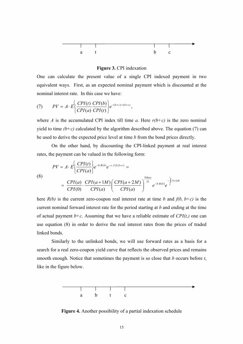
Similarly to the unlinked bonds, we will use forward rates as a basis for a

search for a real zero-coupon yield curve that reflects the observed prices and remains

smooth enough. Notice that sometimes the payment is so close that b occurs before t,

like in the figure below.

Figure 4. Another possibility of a partial indexation schedule

a b t c

a t b c

16

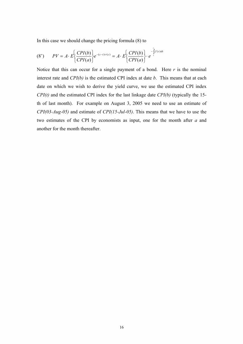
In this case we should change the pricing formula (8) to

(8’) ∫

⋅

⋅=

⋅=−

⋅−−

c

t

dssfcrtc e

aCPIbCPIEAe

aCPIbCPIEAPV

)()()(

)()(

)()(

Notice that this can occur for a single payment of a bond. Here r is the nominal

interest rate and CPI(b) is the estimated CPI index at date b. This means that at each

date on which we wish to derive the yield curve, we use the estimated CPI index

CPI(t) and the estimated CPI index for the last linkage date CPI(b) (typically the 15-

th of last month). For example on August 3, 2005 we need to use an estimate of

CPI(03-Aug-05) and estimate of CPI(15-Jul-05). This means that we have to use the

two estimates of the CPI by economists as input, one for the month after a and

another for the month thereafter.

17

7. CPI linked yield curve, algorithm

The same time grid that we used for calculating the nominal rate is used for

calculating the CPI linked yield curve, however, we included only the points on the

grid which are one year or longer: (0, 1Y, 2Y, 3Y, 5Y, 7Y, 10Y, 15Y, 20Y). The

reason for this is that there are very few CPI linked bonds with a time to maturity of

less than one year.

Assume that we have already found the nominal yield curve (including

forward rates) as described above. We will choose the same grid for the CPI linked

yield curve.6 Again, define the two penalty functions PCPI and QCPI so that PCPI

measures the cumulative price discrepancy and QCPI measures the total degree of non-

smoothness.

As in (6), the total penalty is defined as

(9) )()( CPICPICPICPICPI FQwFP ⋅+

A similar multi-dimensional minimization procedure7 is used to derive the real

forward rates. The resulting real zero coupon yield curve is constructed based on

forward rates (again linearly interpolated between grid nodes).

After a series of tests we conclude that a good balance of smoothness and

price matching can be reached with wCPI=1.

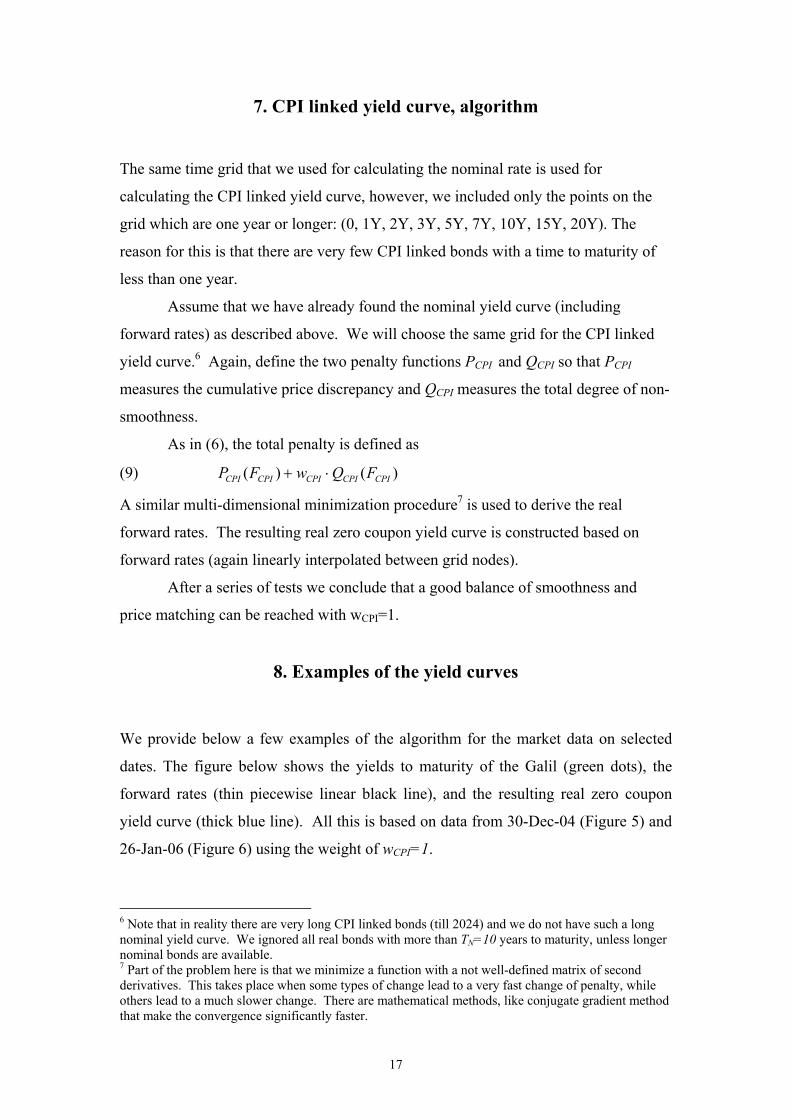
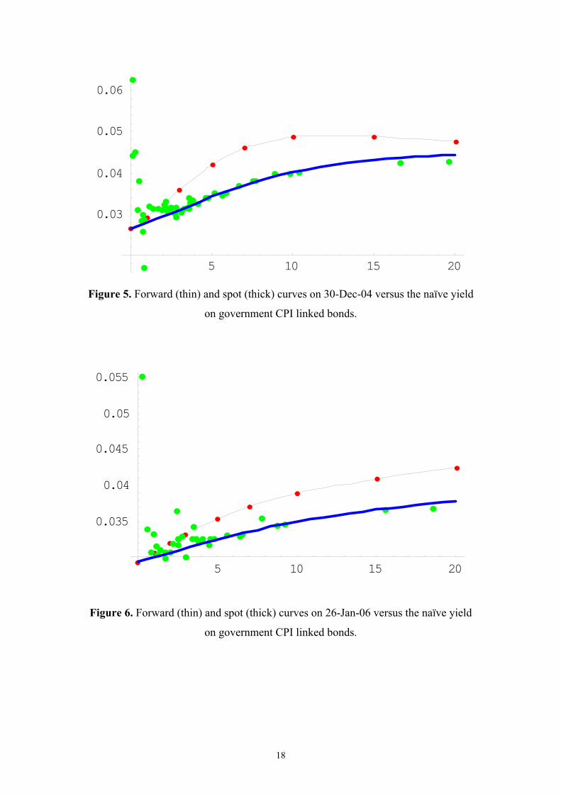
8. Examples of the yield curves

We provide below a few examples of the algorithm for the market data on selected

dates. The figure below shows the yields to maturity of the Galil (green dots), the

forward rates (thin piecewise linear black line), and the resulting real zero coupon

yield curve (thick blue line). All this is based on data from 30-Dec-04 (Figure 5) and

26-Jan-06 (Figure 6) using the weight of wCPI=1.

6 Note that in reality there are very long CPI linked bonds (till 2024) and we do not have such a long nominal yield curve. We ignored all real bonds with more than TN=10 years to maturity, unless longer nominal bonds are available. 7 Part of the problem here is that we minimize a function with a not well-defined matrix of second derivatives. This takes place when some types of change lead to a very fast change of penalty, while others lead to a much slower change. There are mathematical methods, like conjugate gradient method that make the convergence significantly faster.

18

5 10 15 20

0.03

0.04

0.05

0.06

Figure 5. Forward (thin) and spot (thick) curves on 30-Dec-04 versus the naïve yield

on government CPI linked bonds.

5 10 15 20

0.035

0.04

0.045

0.05

0.055

Figure 6. Forward (thin) and spot (thick) curves on 26-Jan-06 versus the naïve yield

on government CPI linked bonds.

19

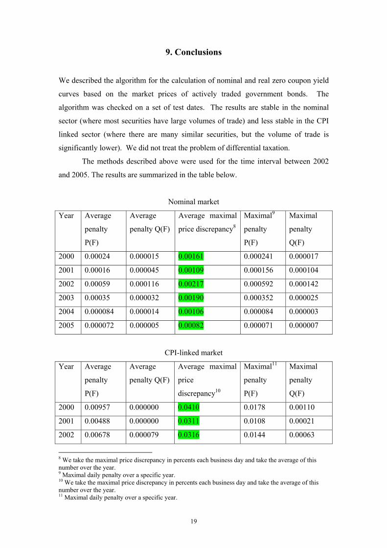
9. Conclusions

We described the algorithm for the calculation of nominal and real zero coupon yield

curves based on the market prices of actively traded government bonds. The

algorithm was checked on a set of test dates. The results are stable in the nominal

sector (where most securities have large volumes of trade) and less stable in the CPI

linked sector (where there are many similar securities, but the volume of trade is

significantly lower). We did not treat the problem of differential taxation.

The methods described above were used for the time interval between 2002

and 2005. The results are summarized in the table below.

Nominal market

Year Average

penalty

P(F)

Average

penalty Q(F)

Average maximal

price discrepancy8

Maximal9

penalty

P(F)

Maximal

penalty

Q(F)

2000 0.00024 0.000015 0.00161 0.000241 0.000017

2001 0.00016 0.000045 0.00109 0.000156 0.000104

2002 0.00059 0.000116 0.00217 0.000592 0.000142

2003 0.00035 0.000032 0.00190 0.000352 0.000025

2004 0.000084 0.000014 0.00106 0.000084 0.000003

2005 0.000072 0.000005 0.00082 0.000071 0.000007

CPI-linked market

Year Average

penalty

P(F)

Average

penalty Q(F)

Average maximal

price

discrepancy10

Maximal11

penalty

P(F)

Maximal

penalty

Q(F)

2000 0.00957 0.000000 0.0410 0.0178 0.00110

2001 0.00488 0.000000 0.0311 0.0108 0.00021

2002 0.00678 0.000079 0.0316 0.0144 0.00063

8 We take the maximal price discrepancy in percents each business day and take the average of this number over the year. 9 Maximal daily penalty over a specific year. 10 We take the maximal price discrepancy in percents each business day and take the average of this number over the year. 11 Maximal daily penalty over a specific year.

20

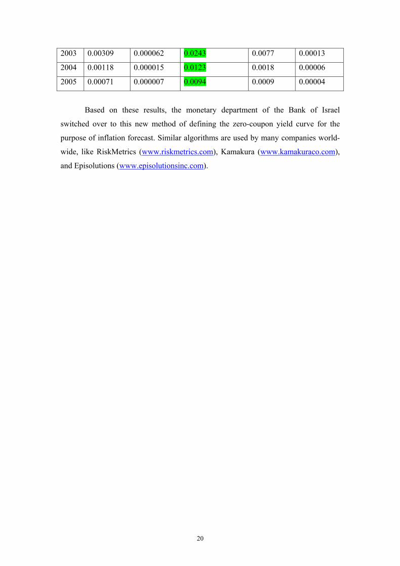
2003 0.00309 0.000062 0.0243 0.0077 0.00013

2004 0.00118 0.000015 0.0123 0.0018 0.00006

2005 0.00071 0.000007 0.0094 0.0009 0.00004

Based on these results, the monetary department of the Bank of Israel

switched over to this new method of defining the zero-coupon yield curve for the

purpose of inflation forecast. Similar algorithms are used by many companies world-

wide, like RiskMetrics (www.riskmetrics.com), Kamakura (www.kamakuraco.com),

and Episolutions (www.episolutionsinc.com).

21

References

Andersen Leif, Yield Curve Construction with Tension Splines, working paper, December 2005, http://papers.ssrn.com/sol3/papers.cfm?abstract_id=871088 Anderson, N., and J. Sleath, “New estimates of the UK real and nominal yield curves”, Bank of England Quarterly Bulletin November 1999, 384-392. Anderson N, and J. Sleath, New Estimates of the UK real and nominal yield curves. http://ideas.uqam.ca/ideas/data/Papers/boeboeewp126.html or http://www.bankofengland.co.uk/qb/qb990403.pdf Bank of International Settlements, “Zero-Coupon Yield Curves: Technical Documentation”, March 1999. Bank of International Settlements, “Zero-Coupon Yield Curves: Technical Documentation”, Monetary and Economic Department, October 2005. Brousseau, V. (2002). The functional form of yield curves, Working Paper 148, European Central Bank. Deacon, M., Derry, A., Estimating the Term Structure of Interest Rates, Bank of England, 1994. Deriving and Fitting Interest Rate Curves Using MATLAB® and the Financial Toolbox, Financial Engineering Technical Brief, www.mathworks.com Evans, M., Real Rates, Expected Inflation and Inflation Risk Premia, Journal of Finance, 53(1), 1998, 187-218. Fisher, M., D. Nychka, and D .Zervos, “Fitting the Term Structure of Interest Rates with Smoothing Splines,” Working Paper 95-1, Finance and Economics Discussion Series, Federal Reserve Board, 1995. Fisher M., and D. Zervos, Yield Curve, in Computational Economics and Finance, ed. H. Varian, Springer 1996, p. 269-302.

22

Gerlach, Stefan, “Interpreting the Term Structure of Interbank Rates in Hong Kong”. Hong Kong Institute for Monetary Research Working Paper,No.14/2001,December. Hagan, P., and G. West, “Interpolation methods for yield curve construction”, unpublished manuscript, November 2004. Hull J., Options, Futures and Other Derivatives, Prentice Hall, 4-th ed., 2000, p. 87-95. Indian term structure, http://www.indiainfoline.com/bisc/iimappr2.html Ioannides, M., A comparison of yield curve estimation techniques using UK data, Journal of Banking and Finance, 27 (2003) 1–26 Maltz, A., Estimation of zero-coupon curves in DataMetrics, RiskMetrics Journal, 3 (1), 2002, 27-39. Monetary Authority of Singapore, “The Term Structure of Interest Rates, Inflationary Expectations and Economic Activity: Some Recent US Evidence”, Occasional Paper No.12, May 1999. Nelson, C.R., and A.F.Siegel, “Parsimonious Modelling of Yield Curves”, Journal of Business, 60, pp. 473-89, 1987. Svensson, L.E.O., “Estimating and interpreting forward interest rates: Sweden 1992-1994”, NBER Working Paper Series, No.4871 (1994). Svensson, L.E.O., “Estimating Forward Interest Rates with the Extended Nelson & Siegel Method”, Quarterly Review, Sveriges Riksbank, 1995:3, 13-26. Vasicek, O.A., and H.G. Fong (1982), “Term Structure Modeling Using Exponential Splines”, Journal of Finance, 37:2, p. 339-348. Waggoner, D., Spline Methods for Extracting Interest Rate Curves from Coupon Bond Prices, Federal Reserve Bank of Atlanta, Working Paper 97-10, November 1997 http://mscf.gsia.cmu.edu/BPM/WaggonerSpline.pdf

23

Wets, R., S. Bianchi, and L. Yang, Serious Zero-Curves, manuscript, available at www.episolutionsinc.com. Yu, I., and Fung, L., Estimation of Zero-Coupon yield curves based on exchange fund bills and notes in Hong Kong, Hong Kong Monetary Authority, 2002 Zangari, P. (1997). An investigation into term structure estimation methods for RiskMetrics, RiskMetrics Monitor pp. 3–31.

24

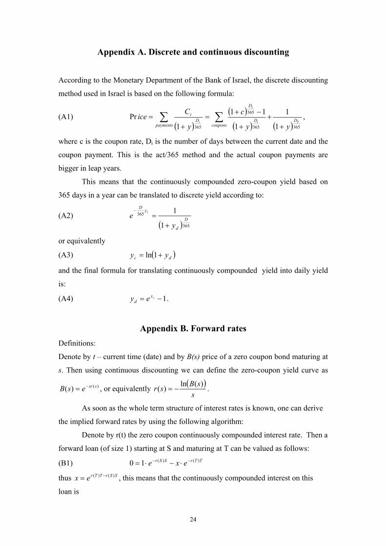
Appendix A. Discrete and continuous discounting

According to the Monetary Department of the Bank of Israel, the discrete discounting

method used in Israel is based on the following formula:

(A1) ( )

( )( ) ( )365365

365

365 1

1

1

11

1Pr

Ti

i

i Dcoupons

D

D

paymentsD

i

yy

c

y

Cice

++

+

−+=

+= ∑∑ ,

where c is the coupon rate, Di is the number of days between the current date and the

coupon payment. This is the act/365 method and the actual coupon payments are

bigger in leap years.

This means that the continuously compounded zero-coupon yield based on

365 days in a year can be translated to discrete yield according to:

(A2) ( )365

365

1

1D

d

yD

ye c

+=

−

or equivalently

(A3) ( )dc yy += 1ln

and the final formula for translating continuously compounded yield into daily yield

is:

(A4) 1−= cyd ey .

Appendix B. Forward rates Definitions:

Denote by t – current time (date) and by B(s) price of a zero coupon bond maturing at

s. Then using continuous discounting we can define the zero-coupon yield curve as

)()( ssresB −= , or equivalently ( )s

sBsr )(ln)( −= .

As soon as the whole term structure of interest rates is known, one can derive

the implied forward rates by using the following algorithm:

Denote by r(t) the zero coupon continuously compounded interest rate. Then a

forward loan (of size 1) starting at S and maturing at T can be valued as follows:

(B1) TTrSSr exe )()(10 −− ⋅−⋅=

thus SSrTTrex )()( −= , this means that the continuously compounded interest on this

loan is

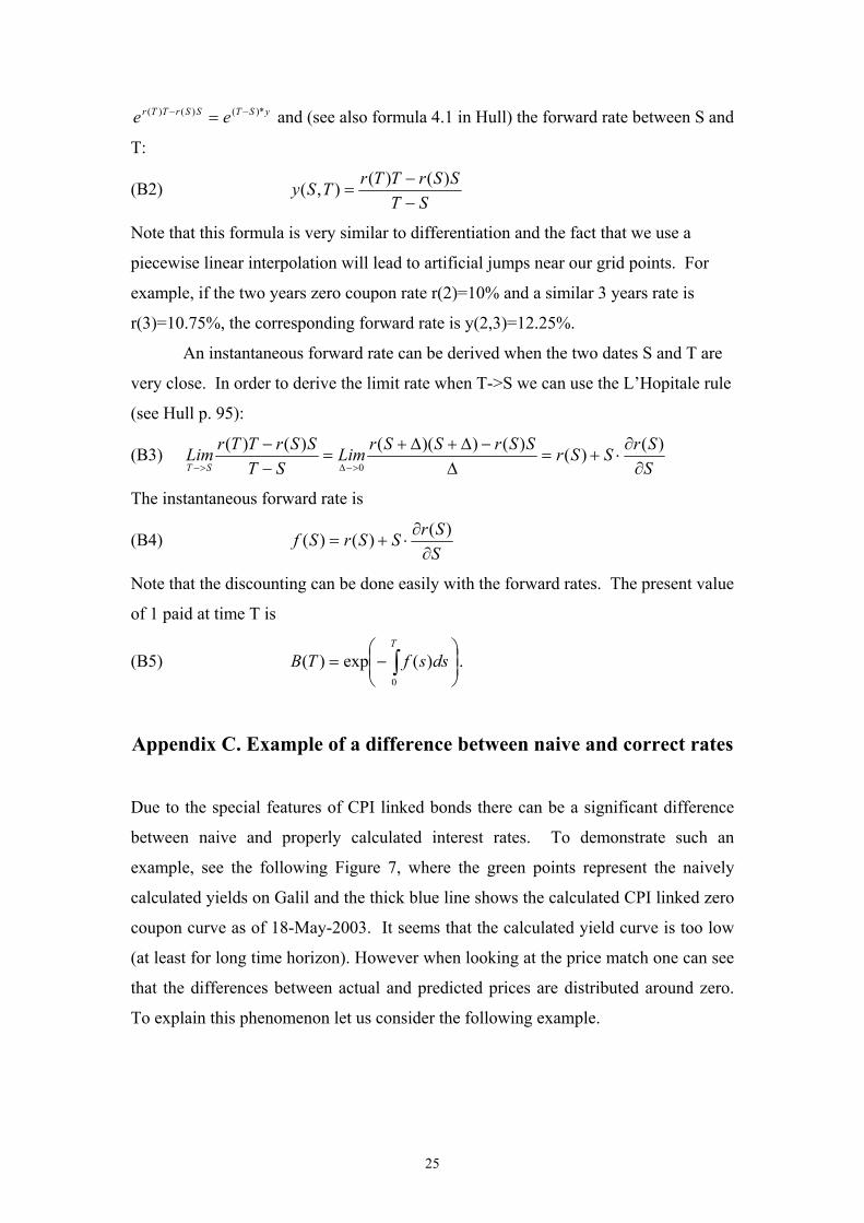
25

ySTSSrTTr ee )*()()( −− = and (see also formula 4.1 in Hull) the forward rate between S and

T:

(B2) ST

SSrTTrTSy−−

=)()(),(

Note that this formula is very similar to differentiation and the fact that we use a

piecewise linear interpolation will lead to artificial jumps near our grid points. For

example, if the two years zero coupon rate r(2)=10% and a similar 3 years rate is

r(3)=10.75%, the corresponding forward rate is y(2,3)=12.25%.

An instantaneous forward rate can be derived when the two dates S and T are

very close. In order to derive the limit rate when T->S we can use the L’Hopitale rule

(see Hull p. 95):

(B3) SSrSSrSSrSSrLim

STSSrTTrLim

ST ∂∂⋅+=

∆−∆+∆+

=−−

>−∆>−

)()()())(()()(0

The instantaneous forward rate is

(B4) SSrSSrSf

∂∂⋅+=

)()()(

Note that the discounting can be done easily with the forward rates. The present value

of 1 paid at time T is

(B5)

−= ∫

T

dssfTB0

)(exp)( .

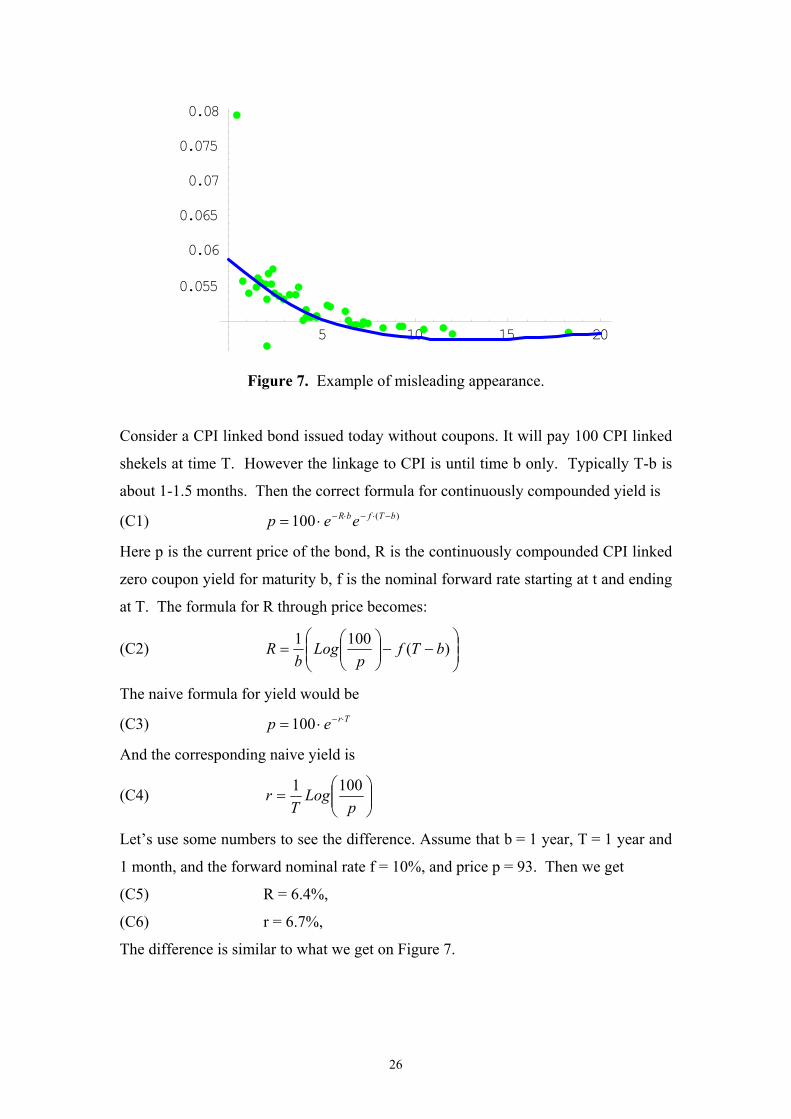
Appendix C. Example of a difference between naive and correct rates

Due to the special features of CPI linked bonds there can be a significant difference

between naive and properly calculated interest rates. To demonstrate such an

example, see the following Figure 7, where the green points represent the naively

calculated yields on Galil and the thick blue line shows the calculated CPI linked zero

coupon curve as of 18-May-2003. It seems that the calculated yield curve is too low

(at least for long time horizon). However when looking at the price match one can see

that the differences between actual and predicted prices are distributed around zero.

To explain this phenomenon let us consider the following example.

26

5 10 15 20

0.055

0.06

0.065

0.07

0.075

0.08

Figure 7. Example of misleading appearance.

Consider a CPI linked bond issued today without coupons. It will pay 100 CPI linked

shekels at time T. However the linkage to CPI is until time b only. Typically T-b is

about 1-1.5 months. Then the correct formula for continuously compounded yield is

(C1) )(100 bTfbR eep −⋅−⋅−⋅=

Here p is the current price of the bond, R is the continuously compounded CPI linked

zero coupon yield for maturity b, f is the nominal forward rate starting at t and ending

at T. The formula for R through price becomes:

(C2)

−−

= )(1001 bTf

pLog

bR

The naive formula for yield would be

(C3) Trep ⋅−⋅= 100

And the corresponding naive yield is

(C4)

=

pLog

Tr 1001

Let’s use some numbers to see the difference. Assume that b = 1 year, T = 1 year and

1 month, and the forward nominal rate f = 10%, and price p = 93. Then we get

(C5) R = 6.4%,

(C6) r = 6.7%,

The difference is similar to what we get on Figure 7.

27

Monetary Studies עיונים מוניטריים

על המוניטרית המדיניות של ההשפעה לבחינת מודל – אלקיים' ד, אזולאי' א1999.011996 עד 1988, האינפלציה בישראל

ביחס האבטלה שיעור של הניטרליות השערת – סוקולר' מ, אלקיים' ד1999.021998 עד 1990, אמפירית בחינה – בישראל לאינפלציה

2000.01M. Beenstock, O. Sulla – The Shekel’s Fundamental Real Value

2000.02O. Sulla, M. Ben-Horin –Analysis of Casual Relations and Long and Short-term Correspondence between Share Indices in Israel and the

United States 2000.03Y. Elashvili, M. Sokoler, Z. Wiener, D. Yariv – A Guaranteed-return

Contract for Pension Funds’ Investments in the Capital Market

לקופות רצפה תשואת להבטחת חוזה – סוקולר' מ, יריב' ד, וינר' צ, אלאשווילי' י2000.04ההון בשוק להשקעות הפנייתן כדי תוך פנסיה

ולחיזוי לניתוח מודל – המוניטרית והמדיניות האינפלציה יעד – אלקיים' ד2001.01

מול תחותמפו מדינות: ההקרבה ויחס דיסאינפלציה – ברק' ס, אופנבכר' ע2001.02מתעוררות מדינות

2001.03D. Elkayam – A Model for Monetary Policy Under Inflation Targeting: The Case of Israel

על השפעתו ובחינת התוצר פער אמידת – אלאשווילי' י, רגב' מ, אלקיים' ד2002.01האחרונות בשנים בישראל האינפלציה

אופציות באמצעות הצפוי החליפין ערש אמידת – שטיין' ר2002.02Call - על שער ה Forward

2003.01

עתידיים חוזים של הסחירות-אי מחיר – קמרה' א, קהן' מ, האוזר' ש, אלדור' ר)בשיתוף הרשות לניירות ערך(

2003.02 R. Stein - Estimation of Expected Exchange-Rate Change Using Forward Call Options

דולר-שקל החליפין שער של הצפויה ההתפלגות אמידת – הכט' י, שטיין' ר 2003.03האופציות במחירי הגלומה

2003.04 D. Elkayam – The Long Road from Adjustable Peg to Flexible Exchange Rate Regimes: The Case of Israel

2003.05 R. Stein, Y. Hecht – Distribution of the Exchange Rate Implicit in Option Prices: Application to TASE

הממשלה של המקומי הגירעון לחיזוי מודל – ארגוב' א 2004.01

28

החליפין בשער חריג ושינוי שכיחה סיכון רמת, נורמליות – פומפושקו' וה, הכט' י 2004.02

2004.03 D.Elkayam ,A.Ilek – The Information Content of Inflationary Expectations Derived from Bond Prices in Israel

התפלגות, דולר-שקל החליפין שער של הצפויה ההתפלגות – שטיין. ר 2004.04 חוץ מטבע באופציות הגלומה פרמטרית-א

2005.01 Y. Hecht, H. Pompushko – Normality, Modal Risk Level, and Exchange-Rate Jumps

ההון משוק לאינפלציה הציפיות גזירת – רגב' מ, אלאשווילי' י 2005.02

הישראלי המשק של מוניטרי למודל אופטימלי ריבית כלל – ארגוב' א 2005.03

2005.04 M.Beenstock, A.Ilek – Wicksell's Classical Dichotomy: Is the Natural Rate of Interest Independent of the Money Rate of Interest ?

2006.01 RND - פומפושקו' וה הכט' י

קטן למשק קיינסיאני-ניאו מודל של ואמידה ניסוח – ארגוב' א, אלקיים' ד 2006.02הישראלי למשק יישום, ופתוח

2006.03 Z.Wiener, H.Pompushko- The Estimation of Nominal and Real Yield Curves from Government Bonds in Israel

המוניטרית המחלקה – ישראל בנק

91007 ירושלים 780 ד"ת

Bank of Israel – Monetary Department

POB 780 91007 Jerusalem, Israel