Embed Size (px)
Citation preview

Loughborough UniversityInstitutional Repository
The estimation ofcumulative noise exposurecaused by aircraft tra�c
This item was submitted to Loughborough University's Institutional Repositoryby the/an author.
Additional Information:
• A Master's Dissertation, submitted in partial ful�lment of the require-ments of the award of the Master Of Science degree of LoughboroughUniversity.
Metadata Record: https://dspace.lboro.ac.uk/2134/10899
Publisher: c© David Brown
Please cite the published version.

This item was submitted to Loughborough University as a Masters thesis by the author and is made available in the Institutional Repository
(https://dspace.lboro.ac.uk/) under the following Creative Commons Licence conditions.
For the full text of this licence, please go to: http://creativecommons.org/licenses/by-nc-nd/2.5/
-------- --- -------- - -- ----
LOUGHBOROUGH
UNIVERSITY OF TECHNOLOGY
LIBRARY
AUTHOR
BR.OWN... P __ _ I
COpy NO. _04bHn./O l_
VOl NO. CLASS MARK
fOR t EFERENCE (NLY
- - - - ~-------

TH8 8STIMATION OF CUMULATIV8 NOIS8 8XPOSUR8
CAUS8D BY AIRCRAFT TRAFFIC
by
DAVID BROWN, B.Sc.
A Master's Thesis
~
Submitted in partial fulfilment of the requirements for the award of
Master of Science of the Loughborough University of Technology
May 1975
Supervisor: J.B. Ollerhead, B.Sc.,M.Sc.,C.8ng.,A.F.R.Ae.S. Department of Transport Technology
~ by David Brown, 1975.

LougnborouJ'l University
of T ~c:'lno!ogy Library
Do". 'l' .. 1 1"l"11. Chu$ ... Ace, 04('1~7../01 No

FOREWORD
The work reported herein has been performed as a
supplementary study within a research programme on
"Public Reaction to Aircraft Noise" under Contract
SN/1170/012 for the Civil Aviation Authority, Directorate
of Operations Research and Analysis.
The main parts of this report (Sections 3 and 4)
evolved from the author's primary responsibility to pro
vide estimates of various noise exposure quantities for
correlation with surveyed community-attitude data. While
these requirements were achieved by means of predictive
techniques based on well-established procedures, there
was obvious scope and need for a more fundamental study
of noise index characteristics in aircraft exposure
applications. This study provided relatively simple ,
relationships for various indices, which can be used
to examine their compatibility and to give a predictive
estimate of one type of index based on information
collected for the estimation of another index type.
These uses are developed herein by reference to example
exposure conditions.

ACKNOWLEDGEMENTS
The author wishes to thank Mr. J.B. Ollerhead, pro-
gramme supervisor and principal investigator, for his
invaluable guidance and support in this and other project
tasks of the research programme. Considerable assistance
has also been given by Mr. Trevor Ingham and
Mr, Tom Aitcheson of CAA (DORA) during their monitoring of
the programme.
This project has been based on noise exposure data
collected and analysed by the staff engaged on the main
research programme and by technician staff of the
University's Department of Transport Technology. Particular .
recognition is due to Dr. R.M. Edwards for his detailed
involvement in both data measurement and analysis, to
Mr. M. Lanzer and Mr. E. Rodgers for their assistance in
preparatory work and participation in the measurement
exercise, and to Miss M. Dredge for computer programming.
The author wishes to thank Miss P. Pilkington and
Mr. Derek Glenister for their production of the typed text
and illustrations contained herein.
"

r
SUMMARY
Community noise caused by aircraft traffic is
examined in relation to its estimation by predictive and
measurement methods. The basic properties of the noise
exposure at any airport-vicinity site are shown to be
mainly defined by the statistics of the peak-level occur
rence and noise duration distributions over a given time
period. The relationship between these distributions is
derived in terms of traffic parameters. This leads to
the derivation of an equation for the evaluation of Leq ,
which makes use of information usually acquired for an
NNI assessment and which is directly comparable with the
NNI formula. An important result of the study is the
development of a simple and convenient method for predict
ing aircraft noise exposures, by which various noise
indices (NNI, Leq , LNP ' LlD' etc.) can be directly
evaluated.

LIST OF CONTENTS
1.0 INTRODUCTION 1
2.0 AIRPORTS AND NOISE EXPOSURE 14
2.1 Air Traffic and Communities 14
2.2 Noise Exposure Caused by Air Traffic 21
2.2.1 Peak Level-based Indices 25
2.2.2 Indices Based on Noise Duration 32
Statistics
3.0 RELATIONSHIPS BETWEEN NOISE INDICES BASED ON
PEAK LE:VEL AND DURATION STATISTICS 37
3.1 The Noise E:xposure Distributions 37
3.2 Noise Indices 42
3.2.1 The Equivalent Continuous Energy 42
Level
3.2.2 The Noise Pollution Level 46
3.3 Summary 49
4.0 THE PREDICTION OF AIRCRAFT NOISE PEAK LEVELS 50
4.1 Introductory Review 50
4.2 An Alternative Method 54
4.3 Aircraft Noise Peak Levels 59
4.4 Noise Propagation at Low Ground Angles 61
, '
LIST OF CONTENTS (CONTINUED)
5.0 NOISE EXPOSURE PREDICTION BY A GRAPHICAL METHOD 67
5.1 The Noise Peak Level Distribution 68
5.2 The Noise Duration Distribution 69
5.3 Noise Indices 71
6.0 MeASUREMENT AND MONITORING CONSIDERATIONS 74
7.0 CONCLUSIONS AND RECOMMENDATIONS 78
TABLES 82
FIGURES 94
APPENDIX I AIRCRAFT NOISE MEASUREMENTS AT SITES 126
NEAR HEATHROW AIRPORT
APPENDIX Il DERIVATION OF NOISE EXPOSURE STAT- 137
ISTICAL DATA FOR A SITE NEAR LIVERPOOL AIRPORT
AND A SITE NEAR MANCHESTER AIRPORT
APPENDIX III ERRORS CAUSED BY NEGLECT OF TRUNC- 139
ATION IN DISTRIBUTIONS OF NOISE EXPOSURE
APPENDIX IV AN EXAMPLE SITE NOISE EXPOSURE 146
PREDICTION
REFERENCED LITERATURE 155
" .', -

1.
1.0 INTRODUCTION
One of the most significant problems facing airport
authorities over the next decade or so, is that of plan
ning for the containment or alleviation of public nuisance
attributable to aircraft noise, while, at the same time,
allowing for an expected increase in air transport demand.
Clearly, there are long-term benefits to be realized with
the supersession of the current air transport fleet by
the larger-capacity, but qUieter, aircraft which are pres
ently in prototype or service introduction stages. For
c?mmunities in close proximity to the runway thresholds of
jet-handling airports, the benefits will be appreciated as
a lowering of the peak noise levels and possibly as an
end to the growth in aircraft movement activity. Commun
ities in the outer region of the airport route zones will
gain an additional benefit of "hearing" fewer aircraft.
There will remain, however, established community regions
where aircraft noise exposure will be rated as excessive
for community comfort. There will be marginal regions
where aircraft noise will be part of a wider problem related
to the overall noise environment encompassing road traf-
fic and industrial noises. It can also be expected that
the development or expansion of smaller regional airports
will bring the airport flight patterns closer to as yet
unaffected residential sites. The ability to assess such
situations, of the present and of the future, and to pro
vide the planning tools by which airport and community
developers can reach amicable decisions, are the primary
•

2.
goals of current studies of environmental noise and its
effects.
The intrusion of aircraft noise into what otherwise
may have been a satisfactory community environment is a
long-established problem; first encountered to the degree
of public reaction by complaint in regions around military
airfields, and later in areas around civil airports where
larger and noisier aircraft, particularly jet-transporters, .
became regular users of the immediate airspace. Although
the problem of community disturbance must have been antici
pated by the aircraft manufacturers and operators the
retaliation by more active public involvement was really
the motive force behind the large-scale inquiry and
-research devoted to finding methods of defining, quanti
fying and controlling this disturbance. The more specific
objectives of these studies were:
(a) to define viable limIts on the noise levels rad-
iated by new and future designs of aircraft during
thei~ airport vicinity operation;
(b) to examine and optimise the flight procedures of
aircraft in the airport zone, with respect to
alleviating their noise burden on exposed commun-
ities while maintaining operational safety, and
(c) to derive a measurable scale of cumulative noise
exposure that would reliably assess the degree of
community disturbance caused by aircraft traffic.
, -I

3. It was intended that the first two of these objectives
would lead directly to a containment of the problem, with
long-term benefits to be realized from the former and more ,
immediate partial relief from the latter. Being concerned
with the noise caused by individual aircraft flights, they
could also be dealt with in some isolation from the third
objective. The last of the above objectives was equally
important in that it would provide a rational planning
tool and a method of noise exposure assessment. Its
applications would be to give legislative control on,
(i) the restricted development of land areas for resi
dential buildings, where the noise exposures are,
or will be in the foreseeable future , unsuited
to this purpose;
(ii) the compensation of residents in excessively
exposed communities, by improvement of the sound
insulation of their homes, and
(iii) the planning of future airports and airport ,
expansions, and the siting of their satellite
communities.
It is somewhat ironical that the seemingly most diffi-
cult and economically most controversial of these object--
ives have been more successfully dealt with than the
others~ Limitations on the noise output by aircraft are \
now an accepted part of the type-certification process
and regulatory methods of aircraft operation in the vicinity
of airports are now part of the flight procedures for many
civil airports. Although cumulative exposure measures

have been derived for aircraft noise, in ~he form of the
tNoise and Number Index t for U.K. airports and in other
4.
forms in other countries, the reliability of the measures
and their applicability to planning decisions of major
importance has been disputed on many grounds, not least of
which is the apparent lack of predictive accuracy in esti
mating the variance of community attitude to aircraft noise.
These particular problems, and other aspects of the subject-
ive effects of noise on communities, have been recently
examined in other Loughborough University studies for the
Civil Aviation Authority (Department of Trade). These are
listed in the referenced literature at the end of this
report.
The present report is confined to an examination of
the methods of estimating, by prediction and/or measurement,
the noise exposure quantifiers that are presently used, or
are proposed for use, for airport noise assessment. An
integral part of this examination is the study of the
dependency of the noise indices and constituent parameters
on the properties of the source and propagation acoustics,
and on the statistical properties of the traffic causing
the cumulative exposure.
Some insight into the purposes and problems of this
particular study is given by briefly reviewing the histori-
cal development of noise scales and exposure indices.
The introduction of the decibel unit as a physical
scale of sound pressure level was reputedly based on the
observation that the human hearing and neurological res-~
, ','t

5.
ponse to impinging sound is of an approximately logarith
mic nature. The subsequent observaions of the inadequacy
of the sound pressure level in predicting hearing responses
at any and all frequencies led to methods of assessing the
loudness of sounds by means of frequency-dependent correct
ions to the sound pressure level spectrum. The better
known of these corrective processes are the frequency-
weighted networks for Sound Level measurement such as the
A, Band C-weighted Sound Level scales. Each of these was
found to be preferable for particular types of nOises, or
noises in particular level ranges. Later investigations
of psychometric scales capable of assessing the noisiness
of sounds, or their disturbance and annoyance-inducing
properties, resulted in many other measurement scales for
steady continuous sounds. All of these studies were con-
ducted by subjective laboratory tests, in which the sound
stimulli and the subject listening conditions could be care-
fully controlled. Similar testing procedures provided a
means of developing noise scales for short-period noise
excursions such as those typical of an aircraft flyover or
an automobile pass-by. Through such tests, the Perceived
Noise Level unit was developed as being best suited to
the definition of aircraft noise levels of any single fly-
over event. For the overall effect of the complete noise
level excursion, it was found that the peak Perceived
Noise Level provides a good correlation with subjective
response (Reference 1). A further development was that
of "Effective Level" which is basically the average-energy
. .;;

6.
level of the excursion over a specified time period. A
slight improvement in the subjective correlation was
obtained (References 2 - 4, for example).
The need for a means of quantifying the subjective
effects of long-term, variable, noise exposures has been
not so readily satisfied. Whereas the former studies were
amenable to controlled laboratory investigations, the cumu
lative exposure problem is not; at least not without
imposing unnatural constnnnts on the study objectives.
Here, the noise exposure is quantified by means of a range
of measurable parameters, and the attitudes of residents to
their local noise environments are solicited by means of
a.questionnaire or by analysis of complaints. This has
supplied the researcher with a bank of experimental data,
from which various empirical noise index forms have emerged
through multiple regressions of noise and attitude para-
meters. The problems of this empirical approach are basic
ally: (a) that the indices have not correlated well with
the total bank of individually-expressed opinions on noise,
although they have correlated very well with the average,
or central tendency, of the opinions in each noise stratum,
and (b) that, being empirical, they are suited only to
domain of their derivation and hence may not be accurate
or appropriate to situations outside that domain. Addit
ionally, it may be argued that some indices derived by
such empirical methods can be insensitive to the needs of
the planner, mainly because they do not give guidance on
how to reduce the noise burden. Thus the problem of
. ' . ) ~
. )
reducing a noise index value, or of diminishing the area
within a noise index contour, can be complicated if the
index formulation does not contain dependencies on phys
ical traffic parameters. Recourse to iterative planning
methods is then necessary. I
By tackling each of the different types of noise
7.
exposure (such as that of aircraft, road traffic, indust
rial plant) in some isolation from each other, it is per
haps not surprising that the social survey regression
methods have given rise to a number of quite different
index forms to suit these different problems. Some
characteristic time-histories of various traffic noise
exposures are shown in Figure 1. The aircraft noise
cases are seen to be a succession of well-spaced (time-
wise) discrete noise events with distinguishable and
readily measurable peak levels. with the knowledge of
this characteristic of airport noise exposure, and with the
benefit of the earlier studies of subjective scaling of !
individual aircraft noise events, the Wilson Committee
(Reference 5) and their associate researchers (Reference 6)
examined the cumulative exposure index problem by analysis
o! community attitude data obtained around Heathrow
(London) Airport. After consideration of many noise para
meters, the final index form was empirically derived by
the Wilson Committee from McKennell's data. This index is
the Noise and Number Index (NNI). It is based on the peak
levels of aircraft traffic noise, measured in Perceived
Noise Level units, and is formulated as, .'
"

8.
NNI = L + lSl0910N - 80 (PNdS) (1.1)
where L is the average peak-energy level and N is the
number of noise peaks 'heard' during an average 12-hour
daytime period.
Although seemingly simple at first glance, the NNI
is in practice a complicated index to evaluate by measure-
ment. An examination of these complications is contained
later in this report (Section 2). However the index form
would seem amenable to the planners' needs in that the
dependence on noise level and traffic number are separable
and directly useful in noise control. Other similar
indices have been independently derived in the U.S.A.,
namely the Composite Noise Rating (CNR) and the Noise
Exposure Forecast (NEF) to be discussed later.
Referring again to Figure 1, it is apparent that the
use of peak level statistics for road traffic (or for
industrial plant noise) exposures would incur severe
measurement and analysis problems. Here the noise is of
a rapidly fluctuating nature and indices for this more
random time history have been derived in terms of ~e
levels exceeded for specific percentiles of time. L10 , .
LSO and L90 are the levels exceeded for 10%, SO% and 90%,
respectively, of the total period of assessment. These
are based on A-weighted Sound Level measurements and were
used in the attitude regression studies concerning London
traffic noise (Reference 7), the Wilson Committee studies
of the same data, and_ in the subsequent work of the
• /
.)

9.
Building Research Station where new social surveys were
performed (Reference 8). Whereas the earlier studies
recommended the use of L10 for road traffic noise expos
ure, the Building Research Station study showed that a
better correlation with community attitude could be obtained
by a more complex index, namely the Traffic Noise Index
(TNI), defined as (References 8 and 9),
TNI = L90 + 4(L10 - L90 ) - 30, dB(A) (1.2)
For numerous reasons, including those of complexity and
the possibility of inherent anomolous properties (e.g.
Reference 10), the TNI was not adopted as a legislative
~ndex. Instead, the L10 over an 18-hour assessment period
has become the present legislative measure of road traf
fic noise (Reference 11) in the United Kingdom. Different
indices have been developed in other countries for th~
road traffic noise problem and for other types of noise
exposure. There is consequently an incompatibility
between the various noise criteria. This is significant
when the noise abatement goals of various countries are
compared and when a comparison between aircraft noise and
other noise criteria is attempted.
Of probably greater significance is that there is no
accepted method (in the U.K.) of assessing a noise expos
ure situation caused by the simultaneous influence of many
different types of sources, including aircraft noise.
Studious attempts to overcome these incompatibilities
have been made in"recent years, particularly by the

10.
International Standards Organisation. The main recommend
ation evolving from the ISO work is that the Equivalent
Continuous Energy Level (L ) should serve as a compatible eq and comparable noire exposure index for general noise assess-
ment. The index is definable in its basic form as
(Reference 12),
L(t)/10 10 • (1.3)
where L(t) is the time history of the A-weighted Sound
Level, averaged on a "Slow" signal averaging system, and T
is the total period of measurement. It can equally be
applied to any other noise scale history, such as PNdB, with
appropriate (approximate) corrections being applied for
comparison purposes.
The L ,as defined above, is the level of a con tin-eq uous unchanging noise that would have the same total energy
as the actual fluctuating noise over the same time period.
Aircraft traffic noise, being intermittent rather than
continuous, does not have a sufficient study background in
such temporal aspects of noise exposure to allow a ready
transformation in assessment applications. The ISO has
therefore examined other forms of Leq that could be more
readily applied to this particular source. One such form,
which is based on the extensive bank of information regard
ing the Effective Perceived Noise Levels of aircraft
flights, is, (Reference 13)
1pN = ~ - 1010910(T/TO), PNiB eq
(1.4)
,
. , ./

11.
where T is the total time period under consideration, and
LE: is the so-called aircraft exposure level given by,
E:PNLi 10
= 1010g10 i
To = 10 seconds and to = 1 second.
When rewritten as E:PNL.
LNP eq = 1010g10 [ ~o 4. 10 101. ], PNdB
where To = 10 seconds is ·the period of the equivalent con
tinuous energy of the highest~dB of each noise excursion,
represented by the EPNL, then the index is seen to be the
long-term average equivalent level of these 10dB range
excursions. Although this index form facilitates its pre
diction by means of established EPNL ratings for the various
aircraft types, and obviates the need for detailed noise
duration computations in the prediction of Leq' it does not
lend itself to monitoring or ,measurement methods capable
of being encapsulated to a single instrumentation 'box',
as does the Leq.
Another index form, proposed by Robinson (Ref. 14), is
the Noise Pollution Level,
(1.5)
where ~ is the standard deviation of the noise level fluct
uations and K is an empirically' derived constant. This
index is based on the concept that there are at least two
12.
properties of noise exposure which cause_annoyance, the
first being the long-term averaged level and the second
being the variability of the noise over the exposure period.
More recently a third property has been examined, that of
the spread of time intervals between noise excursions
(Reference 15).
This brief review of the historical development of
the noire indices presently in use, or proposed for use,
is necessarily incomplete. Many other indices such as the
Leq with night-time energy weighting (Ldn ) are oeing
introduced or are in use abroad. The review given in this
preamble to the following report sections is intended to
~llustrate the diverse nature of the various index forms.
Although at present the only index applicable to aircraft
noise exposure assessments at U.K. airports is the NNI,
there is a growing debate on the need for a unified
index (e.g. References 16 and 17) and a long-established
debate on the need for a modified version of the NNI
(e.g. References 18 and 19).
So, while much of the present report is concerned with
the estimation of airport noise exposure in terms of the
NNI, the apparent need for consideration of the problem
in terms of other index forms is also attacked. Primary /
consideration is given to the problems of obtaining pre
dictive estimates of noise exposure. Although the NNI
has been in use for over a decade, there still seems to
be some diversity in the basic predictive techniques
employed by various consultancy and planning organisattons.

13.
Should some new index be introduced, thi~ diversity of
approach can be expected to widen and to take some consider
able time to be developed into a quasi-confident expertise.
with this consequence taken as worthy of study, the present
work also examines the possibility of deriving prediction
techniques for the other index forms, using the existing
bank of knowledge on aircraft peak noise levels as a sufficient
reference data set.
These practical aspects of the estimation problem
are further reviewed and developed in the following sect
ions. Finally, a specific method of predictive estimat
ion of airport noise is presented. It is readily adaptable
to be an extension of most other NNI prediction methods for
purposes of estimating L1 , LlD' Leq , LNP or other noise
duration based indices.

14.
2.0 AIRPORTS AND NOISE EXPOSURE
2.1 Air Traffic and Communities
The main function of civil aviation airports is that
of a terminal for the convenient arrival and departure of
passenger and freight aircraft which, for the majority of
their travelling time, are operated in controlled air cor
ridors consistent with their most economic route and at
altitudes which cause negligible noise at ground level.
The airspace surrounding an airport serves as a connecting
zone between the runway(s) and the "junction" areas of the
controlled air corridors and it is while traversing this
transitional airspace that aircraft cause noise-induced
disturbance to the local communities. Figure 2 is an
illustrative overview of the air corridors traversing the
U.K., and shows a typical set of traffic control stations
near which an aircraft will join or depart from the cor-•
ridor by changing flight direction, altitude or both.
Between the runway(s) and these intersection areas, the
aircraft routes and altitude variations are controlled
(usually) by the local airport traffic controller and in
many cases will be constrained to an established set of
explicitly-defined routes such as "Standard Instrument
Departure" or "Minimum Noise~' routings and flight proced-
ures. Examp15 of such standard routings are shown in
Figure 3 which illustrates their intended avoidance of
highly populated zones while aiming towards objective air
corridor intersections. Unfortunately, for practical
reasons concerned with air traffic control, flight safety "
" "
"
" . ,

15.
and the avoidance of air space congestion, the routes
cannot avoid all communities. Noise assessment is most
needed in such regions, which may be close to the runways
and thereby exposed to all of the aircraft movements, or
distant from the runways but under a departure or landing
route and thereby subjected only to the aircraft movements
along that route.
The division of the movements into runway-use operat
ions is a pre-requisite for route usage assessments. Many
airports have a 'preferred' runway, that is, except in
unsuitable wind conditions aircraft will normally take-off and
land towards a specific direction of the runway(s) align-
ment. Two examples of a preferential system are:
.. . . . . Unless otherwise required by Air Traffic Control,
Runway 24 shall be used for all movements ~Ihen there is a
head wind component and when a tail wind component is not
greater than 3kts."
.. . . . . In weather conditions when the tail wind component
is no greater than Skts., on the main Runways 28R and 28L,
these runways will normally be used in preference to 10R
and 10L, provided the runway(s) surface is dry. When an
associated cross-wind component on these main runways '.
exceeds 12kts., a runway more nearly into wind will norm
ally be used."
In both examples the preferred movement direction is
due-west, into the prevailing wind. Analysis of these
systems in relation tQ long-term (9-year) summaries of
I t

16.
wind vector statistics for the two example airports indi
cates that the preferred runways would be in use for 79%
and 68% of the time, respectively, which compare well with
the 80% and 62% usage during August 1972 (obtained from
actual runway usage data). This comparison between time
period availability and percentage movement use is rather
tenuous since the former is based on all-year, 24-hour,
statistics whereas the latter is based on three-month
summer season, 12-hour daytime data. However for estimation
purposes where more accurate data on ru~way use is not
available, a 70-30% distribution of movements towards the
preferred runway is representative of typical U.K. airport
conditions.
Route distribution of movements can be treated in a
generalised manner, but requires detailed examination of the
airport traffic statistics and operational instructions.
In many cases sufficient information on defined departure
routes is given in Reference 20 for U.K. airports. Where
information is not so given, recourse can be made to other
publications giving traffic patterns in relation to con
trolled airspace reporting stations (Reference 21). The
more complicated problem is that of distributing the oper
ations among the routes. Here, the~most readily applicable
approach is to cross-reference the mo~ probable route-used
with each flight destination. This form of traffic analysis
can be accomplished by reference to detailed airport-runway
movement data, or by examination of flight-schedules and
• assuming the 70-30% division of runway use.
. ~ "
)

17.
The task of noise exposure prediction is therefore
seen to be preceded by the task of estimating the air traf
fic numbers and fleet-mix which contribute to the exposure
characteristics. The influencing factors which must be
taken into account for traffic-estimating purposes are, in
rank order of importance:
(i) the total numbers of aircraft movements arriving
or departing at the airport within a.specified
period;
(ii) the distribution of these movements with respect
to runway alignment, as dictated by wind condit-
ions;
(iii) the distribution of the movements with respect to
routings associated with each runway alignment,
(iv) the fleet mix of each route-usage;
and (v) further breakdown of the traffic operating condit-
ions where such factors affect noise output and
noise exposure.
Each airport will have unique statistical properties for
each of these factors and will require a separate traffic
analysis. Some general guidelines as to the expected
order of effects can be obtained by review of traffic pat-
terns pertaining at U.K. airports as a whole. Table I is
a summary compilation of such information for selected
airports and illustrates the individuality of each airport's
traffic.
The air transport statistics given in the table include
.' ",I<{'( ,
18.
landing and take-off events of passenger-and freight air
craft, but do not include events caus~d by test and training
programmes or by movements of empty aircraft between air
ports. These latter events must obviously contribute to
the local noise exposure and in some cases may tend to
cause most annoyance because of the concentration of (train
ing) flights into short time periods. Such movements should
therefore be included in the definition of th~ airport traf
fic matrix for noise estimation purposes, either by
retrospective assessment or by projections of airport usage.
So far in this section the discussion of airport traf
fic has been limited to the spread of aircraft flights
across the map of an airport region. It is obvious that
the line-routes shown in the Figure 3 examples can only be
regarded as a first-order approximation to the dispersal
of departing traffic. In reality the aircraft follow these
defined routes, but with some degree of lateral scatter
about them. Since the noise level caused at a site by an
aircraft flyby is dependent on the distance between the site
and the aircraft, this lateral scatter must induce some var
iability into the overall traffic noise exposure, even if
all the departing aircraft are of the same type. There are
many other causes of variability (in 'addition to fleet-mix).
Atmospheric effects on sound propagation are an obvious
example, but are usually neglected in favour of a 'standard
day' atmospheric model. Of greater significance is the vert
ical spread of the departure flight paths. For any particular
departure flight, the height profile of the flight path
t

19.
will depend on the performance capabilities of the air
craft type under its loading conditions for the trip, on
the noise abatement procedures dictated by the airport
for the route used and on any height limitations imposed
on the route usage for air-traffic control purposes. The
last two of these are usually defined in literature govern
ing airport use conditions (e.g. References21,22 and 23).
The noise abatement procedures are usually defined by
reference to the peak noise levels allowable at noise
monitoring points (NMP) stationed under and to the side of
the routes. The air-traffic control limitations are usually
defined as a height at which, or above which in many
cases, the aircraft should cross one of the navigational
beacons (such as Burnham, Epsom, Ockham, Woodley, etc.,
in Figure 3(b».
Considerable study has been made of methods by which ,
this height profile spreading can be modelled for noise
prediction purposes, with adequate definition given without
detailed and laborious examination of each flight and of
the aircraft's performance. The most notable of these
models were derived by Bolt, Beranek and Newman Inc. (USA)
under con,tract to the U.S. Federal Aviation Authority
(References 24, 25 and 26 for example). The more recent
of these is shown in Figure 4 and Table II where the
height profiles are categorised and applied to a flight
model according to the aircraft type and its destination
range (which determines the fuel loading and hence the
maximum climb rate capability). The noise abatement climb .~
\
" . .:: ~.' 'I

20.
rate is often taken as a fixed percentage of the maximum
rate, as is the climb-to-cruise level rate. In recent
work by Loughborough University on other aspects of noise
exposure, these percentage rates have been taken as 40%
and 60% respectively. The positions along the flight
paths at which these power changes occur will depend on
the airport controls. Typical of these is a cutback of
power at 5.3km from start of ground run and a resumption
of climb power at a height of 910 metres (3000ft.).
With all of the above prerequisite information com-
piled for a noise exposure prediction exercise, the task
of noise level calculations for any particular site or
for iso-noise contours around the airport can commence.
This is best handled by means of a digital computer with
large storage capacity. Various processing logics can be
developed for such work. One such programme has been
developed by the present author and his associates for
the estimation of noise exposure around many U.K. airports
(see preliminary referenced literature list). A typical
listing of the input traffic data to this programme is
shown in Table Ill. Here, the aircraft types, destination
ranges, routes and climb profiles have been categorised and
the corresponding average number of events in each category
combination is used as the traffic statistic. This method
follows closely that of References 24 - 26, although the
programme detail is designed to be very flexible such that
many different noise exposure indices and parameters (inc-
luding NNI, L10 ' Leq' ~NP) can be computed in contour form.
"
>,
•
" "

21.
There are clearly many other approaches to the stat
istical description of airport traffic. The above dis
cussion is mainly of a quasi-deterministic approach with
distinct divisions in the event models. A more realistic
model would probably be that of a continuous distribution
of the traffic (types, heights, lateral distances, etc.)
relative to a site or line flight path. It is the
author's contention that a much more simple and similarly
accurate method is that in which the traffic statistics
are basically those of route-usage and fleet mix, all
other dispersion effects being incorporated in the tech
nique for noise level calculation. This is developed in
the following sections of the present report and in the
noise prediction method presented in Section 5. It is
still essential, however, to have an in-depth knowledge
of the air traffic characteristics and imposed limitations
on operations before embarking on a noise exposure assess-
ment of any community environment.
2.2 Noise Exposure caused by Air Traffic
The noise exposure experienced by a community is
fundamentally the time history of the noise level fluctu-
ations over a very long period. Noise exposure indices
are intended to provide a single-valued rating of this
exposure, taking account of the subjective influence of
the exposure on the community residents and of as many
characteristics of the time history as is necessary (and
convenient) to obtain an accurate rating of this influ-
ence. The indices must be amenable to measurement,
" '

22.
prediction and noise-abatement interpretation in order to
satisfy all of their intended purposes. In the intro
ductory section to this report it was shown that aircraft
noise exposure indices, either in present use or being
considered for use, fall into two forms. One form is ,
mainly dependent on the statistical distribution of peak
noise levels, and the other form depends on the distribut-
ion of durations of the noise above various levels. These
are now examined with reference to specific examples of
statistically analysed data obtained for regions around
HeathrO\. (London) Airport and for Manchester and
Liverpool airports. As extensive use of these data is
made in this and subsequent sections, a description of the
means of acquisition, analysis and compilation is sepa-
rately given as Appendices to this report. These
appendices should be read in order to gain a full under
standing of the data-interpretation discussed here and
elsewhere in the report.
Figure 5 is a graphical presentation of statistical
noise data obtained by analysis of tape recordings of
aircraft events, acquired over a 12-hour daytime period
at three sites near Heathrow (London) Airport. Two of
the sites were close to departure routes and the third
site was close to the 3-degree glide slope approach path
of one runway. The data for each site are plotted accord
ing to the percentile of peak level occurrences and the
percentile of the 12-hour time period, respectively, for
which specific noise levels were exceeded., These noise
. " ;.-

23.
levels were measured in dB(D) units and are presented in
units of dB(D) + 7dB, which approximates to PNdB units
(but see later comment on this). step increments of 5dB
were used in the analysis.
As a further explanation of the Figure, consider the
two sets of data corresponding to the Site 3 exposure.
Taking a vertical line through the 10-percentile base
scale to intercept the interpolation lines through the
upper and lower data sets (for Site 3) we obtain the level
which was exceeded by 10% of the noise peaks and the level
which was exceeded (by the time history) for 10% of the
12-hour period. In the notation used in this report, "-these levels are L10 and L10 respectively. The latter is
in common w~th tne no~se durat~on based ~na1ces rev~ewea
earl1er.
The base scale of Figure 5 is Gaussian incremented
about the 50-percentile reference, such that any Gaussian
distribution of data would be represented on the graph'by
a straight line. It is apparent that the noise data mea-
sured at the three Heathro\o[ sites can be approximately
described by Gaussian distributions of peak levels and of
noise durations. These descriptions must be qualified by
noting that both distributions (for any site) will be
truncated at some upper noise level which is not exceeded
by any noise peak. The effect of this truncation on index
evaluations is discussed later in the text and in an
Appendix.
Before elaborating on these apparent Gaussian prop-

24.
erties of the distributions, it is necessary to examine
other noise exposure cases where the total number of flights
is typically much less than that at Heathrow. These are
presented in Figure 6, the noise data being graphically
shown in the same format as those of Figure 5.
The Figure ~ data cases are based on the Site 3
Heathrow noise measurements, which are shown again for
reference purposes, but are derived for equivalent sites
near Manchester and Liverpool Airports (see Appendix II).
The derivations make use of actual runway movement logs
from these airports, noise data for each of the flights
being extracted from the Heathrow measurements for the
identical aircraft type and destination range. They are
therefore simulations of noise exposures which would be
caused at some sites near the two airports, of identical
proximity to flight routes and runways as is Site 3 to the
Heathrow Airport routes and runway(s), and assuming identi
cal flight procedures at all three airports. The validity
of these assumptions is unimportant to the interpretive use
that is made of the data.
Of greatest significance in comparison of the three
airport cases is that whereas the peak levcldistributions
apparently retain their approximately Gaussian property,
the noise duration distributions do not. This is examined
in some detail in Section 3.1 where an analytical expression
for the duration distributlon is derived. Meanwhile a more
general and conceptual interpretation of these data proper
ties is made by considering ~he vario.us forms of noise

25.
exposure indices and their dependence on the distributions.
2.2.1 Peak Level-Based Indices
Indices based on noise peak level occurrences are
the Noise and Number Index (NNI) and the Composite Noise
Rating (CNR).
NNI = L + 1510g10N 80,
CNR = L + 1010910Nf - 12,
PNdB
PNdB
(2.1)
(2.2)
The first is that used in the U.K- for aircraft noise
exposure assessment and is based on the number· of flights
"heard" and on the average peak-energy level of these N
events, L, given by,
L = 1010910 [ ~ t.: 10 J (2.3)
In its accepted use, it is applicable to assessment by only
considering flight events occuring during the daytime
12-hour period between 0600 and 1800 hours GMT. The CNR is
similarly based on Land N but is a 24-hour assessment
index with higher weighting given to the number of night
occurrences of events.
=
where Nd is the number of exposure-contributing flights
within the period 0700 to 2200hrs. and Nn is the corres
ponding number within the period 2200 to 0700hrs. (local
time) •
The CNR was derived (1964) in the U.S.A. for appli
cation to regions around military airfields there. Its
use for civil airport regions was given extensive study,
, •• -"i
, I
I

26.
but due to the later derivation of the Effective Perceived
Noise Level (EPNL) and its adoption as a regulatory measure
of individual aircraft noise, the CNR was not formally
used for the civil airport problem. Instead the Noise
Exposure Forecast (NEF) is used.
NEF = EL+ 1010gNf - BB, EPNdB (2.4)
where N EPNLi
[ 1
~ 10
J EL = 1010g10 N 10 (2.5)
No~noting the form of L in equation (2.3) as containing
an average of weighted peak levels, it is clear that it
can be evaluated directly from the peak-occurrence'distri-
butions of Figures 5 and 6. Thus,
<>0 A
i LIlO A A
10 .p(L).dL o
(2.6) ] J\
where p(L) is the probability density function of the
'continuous' peak level distribution.
If a Gaussian distribution is used to describe the peak
level statistics, then, by substituting
1\ 1 p(L) = -~- exp
~p
" " 2
[ -(L - LSO) J
2.,.-2 P
1\ where LSO is the 50 percentile level and ap is the stand-
ard deviation of the peak distribution, the result is
obtained,
L " CT"p2
= LSO + B.68 (2.7)
- .
, .' > '

27.
which is (now) well known in its equivale~7 form for Leq
(discussed later). The assumption of the infinite limit
in the integration and the potential error incurred by
this, is examined in Appendix III. Equation 2.6 can be
expressed as, 0<) 1\ U 10
LilO " ] L = 1010g10 • dP(L) (2.8)
which is suited to graphical integration of the Figures 5
and 6 peak occurrence statistics. In the present notation 1\
100xP(L) is the percentile (base scale) of the figures
" corresponding to any level L. In summation notation, for A
increments of 5dB in L,
-L = 1010g10 L i
J\
[ Li / 10 LlD
...... (2.9)
(A correction of approximately ldB should be added to the
result of this estimate, to account for taking the arithmetic A
centre of the L stratum instead of the geometric centre.)
There is, however, a complication involved in using this
definition of L in the NNI equation 2.1. This arises from
the use of term "number heard" in the original derivation of
NNI (Reference 5). In the later (1967) survey of Heathrow
Airport noise (Reference 18) the NNI evaluations were based
on peak levels which exceeded 80PNdB. This lower limit of
significance has become adopted as a standard approach for
NNI assessments. From the viewpoint of obtaining L by , -
graphical means from the peak-occurrence statistics, the

, ,
28.
80PNdB limit poses no severe difficulty. In u5ing other
methods, such as Equation 2.7, the incurred error can
become large depending on the standard deviation of the
distribution. Figure 7 shows how L varies with change in
the cut-off level of significance (A) for one of the
measured data cases of Figure 5. In this example LA was
evaluated by direct energy averaging of the population of ~ Li values, rather than by distribution integrating or other
methods. It is seen that in the example case there is
little contribution to L made by peaks below 80PNdB.
Energy-averaging gives higher weighting to the higher
levels. A lower standard deviation (or a lower slope of
the Figures 5 and 6 distribution lines) would change the
emphasis of the weighting, but this would seem unlikely
now in the light of the three airport cases.
Returning now to the air-traffic influence on noise
exposure, it might be expected that the peak level distri
bution is quasi-stationary (in the statistical sense) for
any particular site near a particular airport. Hence it
would be expected to be independent of the total number of
aircraft events and mainly dependent on the typical fleet
nix using the nearby route(s). L would be then expected
to be invariant with time, prov~ded of course tnat a
typ~cal route usage occurred •.
Figure 8 shows measured cumulative-period values of
the average peak-energy level and NNI after each hour of
a 12-hour period at 2 sites near Heathrow Airport. As
would be expected, the average level approaches its final

29.
(12-hour) value more rapidly than does the NNI, because
of the increasing cumulative counting of the number para-
meter. However, it must be noted that even for a site near
a very busy airport route a minimum of 5 hours of continuous
monitoring was required to obtain an estimate of the aver-
age level within ldB of the final level. Individual hourly
averages over the day were scattered over a range +4,
-6.5dB at Site l)and +3.5, -4.5dB at Site 2. Thus it is
clear that abbreviated sampling methods are not suitable as
an alternative to the 12-hour averaging process. The NNI
is a long-term averaged rating and is required to be esti-
mated for a month or three-month "average" mode of operations.
In order to examine the properties of the NNI over such a
long period, recourse has been made to a noise prediction
method by which the 12-hour values of NNI, average peak
level, and the number parameter, have been estimated for the
following airport operations cases at Heathrow Airport:
(a) the actual runway utilisation data for different
days during August 1972, including the 'worst' cases
on total movements and on movements in specific
directions and routes;
(b) a runway utilisation case derived by averaging all
movements of specific aircraft, by route and a load
ing factor, over a month of August 1972; and
(c) the actual runway utilisation data for the 12-hour
daytime period of April 10, 1973.
The latter corresponds to the measured data cases "

30.
which were acquired on that date at the three sites
around Heathrow Airport.
The data obtained by these prediction and measurement
exercises is compiled in Table IV. It is seen that good
agreement has been obtained between the measured and pre-
dicted values of average peak-energy level for the three
sites, and that very little variability has been predicted
in the values of this noise parameter at each site over the
fairly wide range of operations numbers. Based on these
results, which do not allow for variations caused by extreme
atmospheric effects such as high wind velocities and
large-scale temperature inversions, it can be reasonably
concluded that the Noise and Number Index contains a fairly
stable parameter, the average peak-energy level, which is
amenable to both measurement and prediction. From the
measurement viewpoint, a single day m~asurement exercise
would suffice to provide an estimate of L in a long-term NNI
assessment.
Of greatest significance is the typical fleet mix using
the route(s). Similarly, the peak level distribution can
be regarded as stable and amenable to both measurement and
prediction. One point of note to the measurement aspect,
however, is the complexity of measuring in the Perceived
Noise Level scale. The computational complexity of this
scale requires a very laborious processing of the contin
uously changing sound pressure spectrum, in f-octave or
octave band levels. This demands the convenience of
digital computing facilities either on-site, or for later •
.-

•
31.
processing of accurately recorded data. For peak level
data it has been found that a good approximation to the
peak Perceived Noise Level is given by the peak D-weighted
Sound Level plus 7dB. In an extensive study of community
noise (reference 27) this approximation was tested for
over 4000 samples of aircraft noise events. The standard
deviation of the error was 1.SdB over the total sample
population. For NNI monitoring purposes this much simpler
measurement process is now widely accepted as adequate.
From the noise exposure prediction vie~lpoint, the stab-
ility of the peak level distribution can be used to
some considerable advantage in estimating L, NNI and other
indices such as L1 , L10 , Leq and LNP ' This is developed
in sections 3, 4 and 5 of the present work.
The number parameter in the NNI, 151og10N, can present
more difficult problems in the measurement or prediction
process, because of the SOPNdB cut-off. In the Figure 7
example a consistent error of 2dB, say, in the measurement
of th~ peak levels would have introduced a 2dB error in L
and about ldB in 1510g10N, giving a total error of 3dB in
NNI. However, reference to the statistical distributions
of Figures 5 and 6, and consideration of these at lower
levels (by a downward translation of the data), illustrates
that the 2dB error could introduce an error on 15log10N of
4 to 5dB. This would give an error of 6 to 7dB on NNI.
Clearly such cases would only occur where the NNI was of
low magnitude, less than 20 say. ThE error potential
should aiways be carefully examined when it is necessary to

32.
predict or measure low order NNI values. Recourse to the
distribution analysis provides a clear method of such exam
ination.
2.2.2 Indices based on Noise Duration Statistics
Level exceedence statistics are obtainable from noise
histories by means of analogue or digital processing equjp
ment. The most common form of output from such analysis is
of cumulative time counts, giving the time over which the
noise history exceeded pre-set levels (most often in 5dB
level increments). From these, the percentile duration
above each level can be calculated and p~esented graphically
as shown in the examples of Figure 5. The statistical
levels L10 , L50 , etc., can be interpolated from the graphs.
The main application of level-exceedence statistics has
been to assess road traffic noise. In a study of the
relationships between this type of noise and the attitudes of
communities to it, it was found that the correlation coef
ficients of the regressions were 0.6, 0.45 and 0.26 for L10 ,
L50 and L90 respectively. Multiple regression of these
levels with the attitude data indicated a significant prefer
ence to an index based on L10 - 0.75L90 , from which the
Traffic Noise Index was derived. The correlation coefficient
for the TNI was 0.88.
In the U.K., the L10 (18-hour) has been recently form
ally adopted as the regulatory measure of noise exposure due
to road traffic noise. In the U.S.A., the noise assessment
guidelines used by the Department of Housing and Urban
Development for general noise environments {excluding air-

33. craft) are based on the level exceedence criteria (refs. 28,
29) as follows:
Unacceptable:
Exceeds 80dB(A) for 60 minutes per 24 hours, or
Exceeds 75dB(A) for 8 hours per 24 hours.
Discretionary (Normally Unacceptable):
Exceeds 65dB(A) for 8 hours per 24 hours.
Discretionary (Normally Acceptable):
Does not Exceed 65dB(A) for 8 hours per 24 hours.
Acceptable:
Does not Exceed 4SdB(A) for more than 30 minutes
per 24 hours.
As it is difficult to meet the last criterion even in remote
rural countryside (see Reference 30), the usual distinction
between acceptable and unacceptable (as applied in the
U.S.A.) is that of 6SdB(A) for 33% of a 24-hour period.
If it is assumed that night-time noise is of a lower level,
then for the eighteen-hour period of assessment used in
the U.K. (for road traffic noise) this would correspond to
a limit of L44 equal to S4dBA). The U.K. limit is L10
equal to 68dB(A).
Another way of examining or comparing the various
noise duration criteria is to consider them all as elements
of a limiting distribution. This is shown in Figure 9 where
a Gaussian distribution line criterion has been drawn through
the L10,LSO and L90 limits (between acceptable and unacceptable
.'

34.
for each) given in Reference 8 work for 24-hour exposures.
The U.S. HUD limit, and an aircraft limit of 92PNdB at Lo~'
have also been included. Also shown is a similar criterion
line derived and proposed by Schultz (Reference 31). The
interpretation and use of the line-distribution criterion
is that if any actual (measured) distribution of noise
level exceedences breaks through the limiting line, ,then
the exposure would be assessed as unacceptable. It is
interesting to note that if the limiting line is taken as
an actual exposure distribution, the values of TNI, Leq
and LNP for the exposure agree very closely with the
centroids of regression obtained by re-analysis of the
road traffic survey data. This re-analysis is reproduced
as Figure 10 of the present report and is contained in
Reference 30 based on Reference 8 results. It may be pos
tUlated that such a limiting distribution criterion
provides both necessary and sufficient conditions of
acceptability. The constituent elements, such as L10 or
LSO ' are only necessary conditions. From a practical
viewpoint it would be desirable to place some constraints
on the extent to which the distribution should be extrapo
lated. The Ll level, which would be the level exceeded
for about 7 minutes of a 12-hour period, would include the
worst cases of aircraft noise. Without such constraint,
the criterion would apply also to impulsive (transient)
noises such as quarry-blast explosions and sonic booms.
"
, '
Consideration of the L10 or higher-percentile levels
in relation to the aircraft noise data of Figure 6 clearly
indicates the inappropriateness of such indices 'for the
airport exposure case. A lower percentile level, such as
L1 , might be useful but there is no real evidence to sup
port this contention. The use of the limiting distribution
(Figure 9) or a family of such distributions each with a
rating value for assessment purposes, would appear to be
viable. Of the noise duration distributions presented in
Figures 5 and 6, those which violated the Figure 9 criterion
had NNI values in excess of 35NNI. Other sources of
noise (road traffic, industrial plant, etc.) could easily be
assessed in isolation from each other or as a total com-
bined environment (including aircraft contributions).
Of greater interest, at present, is the potential use
of the Equivalent Continuous Energy Level, L ,for individeq
ual and combined noise source fields. One of the benefits
of such an approach is that Leq values for individual source
fields (measured over the same time period and in the same
units) can be energy added to give the overall Leq. Thus a
measured or predicted value of Leq for aircraft noise over a
12-hour period can be compared with Leq values for other
sources operating in the same period, or energy added to
them to obtain the overall value.
The basic definition of Leq was given in section,l,
Equation 1.3. In the same way as the average peak-energy
level is obtainable from the peak-occurrence distribution
;
, .

36.
(Equations 2.6 and 2.8), so also is Leq
noise duration distributions. Thus,
obtainable from the
= [ 100 LIlO l 1010910 0 10 .p(L) .dLJ (2.10)
where p(L) is the probability density function of the
noise duration distribution. The graphical integration
methods discussed in Section 2.2.1 are equally applicable
to Leq. Recourse to the Gaussian approximation form of
Equation 2.7 cannot be confidently made in all the Figures
5 and 6 cases. Unacceptable errors would be incurred in
the Manchester and Liverpool cases for example.
The difficulties associated with the prediction or
noise abatement interpretive use of Leq are:
(i) its estimation requires detailed knowledge of the
noise duration distribution;
(ii) this distribution is sensitive to the number of
aircraft involved in the noise exposure, but this is
not explicit in the index formulae;
(iii) there is no clear method of interpreting how to
reduce a level of Leq.
These difficulties are resolved in the next section, with
specific consideration of aircraft noise exposures.

37.
3.0 RELATIONSHIPS BETWEEN NOISE INDICES BASED ON PEAK
LEVEL AND DURATION STATISTICS
In the preceding sections a review has been made of
some of the basic characteristics of noise exposure due to
aircraft traffic sources and of the noise indices currently
used (or proposed) for assessment of noise exposures. It
has been shown that many of the noise indices can be eval
uated by reference to the statistical distribution of either
the peak level occurrences' or the level-exceedence durat-
ions. In this section the relationship between these
distributions is examined for aircraft noise exposures, and
the corresponding dependencies between noise indices are
developed.
3.1 The Noise Exposure Distributions
The aircraft traffic noise environment is considered as
a succession of individual and separable noise events, in
which the overlap of the noise level excursions can be
neglected. Further, the statistical distribution of peak
level occurrences is considered to be known (or readily
predictable by existing estimation methods') and to be
adequately approximated as Gaussian. It is also worth noting -again that the peak occurrence distribution is relatively
stable (invariant) with respect to time (in the day-to-day
sense) and thetotal number of daily movements at the
airport. The main dependency (other than distance to the
flight route) is that of fleet-mix.
'See Section 4.0 for examples.
, I

38.
The problem to be tackled here is to derive a defin-
ition of the statistical properties of the level exceedence . . durations, based on knowledge of the peak level distribut
ion and other parameters. The inverse problem is well
known in other topics such as cumulative fatigue damage of
structures, but is based on the existence of Gaussian
properties of higher order than can be assumed for the pres-
ent work. Instead, a much simpler model of each noise level
excursion is used here to obtain a solution.
Consider a single noise level excursion caused by an
aircraft travelling along a straight line path with a mini
mum slant range distance h from the (noise-exposed) site
(Figure 11(a». , A
The peak sound level at the site is L,
caused by the aircraft at its closest approach point. The
directivity of the sound level radiated from the aircraft ,
is assumed to be spherically uniform when measured in dB(D)
or PNdB (as shown in Reference 32).
The time history model to be used is a symmetrically
triangular sound level excursion, by which the duration of
the sound above a level A is given by,
" t).
2(L-A) (3.1) =
I ~~ I as shown in Figure 11(b).
Now the sound level caused by the aircraft at some
other radius r is:
1\ 10log(r/h)k L(r) = L(h) -
,. ,
. I

39.
where k is the propagation exponent, usually taken as equal
to 2.67 (for 8PNdB attenuation per distance doubling) for
air-to-ground propagation. Neglecting retarded time
effects, we have
" L(t) = L
for the time history,
k/2 1010910 (1 + a2t 2 )
where a = U/h, U is the aircraft speed. Hence,
10 ka 2.31 (3.2)
Figure 11(c) shows the manner in which the bracketed term
varies with at. Of particular interest is the average
value between the peak (at = 0) and various at. It is
seen that
at '\ + (at)ij
= 3.0
will give a reasonable approximation. Substituting this
in (3.2), equation (3.1) becomes,
t). 2(L -A)
I ~~ I " (L -A)
0.6Ska (3.3) = =
Now, for N aircraft events whose peak levels are continuously 1\
distributed with probability density p(L), the total time
for which the level A is exceeded can be expressed as,
00 •
I (t ->. ) 1\ 1\ N 0.6Ska .p(L).dL
J. -
T). = (3.4)
The use of an infinite upper limit in this equation is
of course questionable, because we know that there is always
a finite truncation of the peak level distribution. This
point, and its consequences on the developed results, are
.' • ' >

40.
examined in Appendix Ill. The infinite limit is retained
here for simplicity of integration. It is also worth
noting that the development of the model can be further
simplified by taking the average value of ka as applicable
to all events on a particular route.
Hence the fraction of time for which A is exceeded,
when the N events occur within the total co
I T" NI (I.. - >. ) A A P(I\) = T = T 0.65ka .p(L).dL
"
time period T, is,
(3.6)
Substituting the Gaussian distribution model of the peak
level occurrences this becomes,
N 1 f ' -(L - L50)2 0.6Ska peA) = T. (L-A)exp.( 2 )dL
J 21T' <T 2 U:p P >. .
••••••••••• (3.7) A
where LSO is the average peak level and op is the standard
deviation of the peak level distribution. ~lith
A '" u = (L-LSO)/op equation 3.7 b~comes
0.6Ska peA) = ~. J ~1T' J [opu +
_ L$'o-).. op •••••••••• ,
with the resultant expression for peA) as:
'" A N (LSO -)..) [ LSO - ~ ]
0.6Ska peA) = T 2 l+erf( ) A /Fa-
H 2 P <r:.
+ ....:..E.... exp . J 2'tr
-(LSO -A) ( 2) 2cp
.du
(3.8)
(3.9)
This equation can now be used to give an estimate of peA) x
100%, which is the percentage of the total time period T
'for which the level'~ is exceeded. The distribut-
, ,
'""
't ,~ , -' 'I! '.

41.
but ion of peA) can be drawn, or by inserting a percentile
value the corresponding level of A can be estimated. Thus
by inserting peA) = 0.5, the resultant A is LSO ' etc.
The information required for such evaluation is:
" (1) LSO and a- for the peak level occurrences; .p
(ii) the number of events occuring in the time period;
(iii) the average value of a = U/h for the aircraft
route, and
(iv) the propagation exponent, k, appropriate to the
site position relative to the flight path.
Taking k = 2.67 (8dB per distance doubling) and T =
3.6 x 10³ seconds, N becomes the average number of flights
per hour. The expression (3.9) becomes,
•••• (3.10 )
where n is the average number of flights per hour and
a = U/h in units of 1/ seconds'
An obvious and available test on the validIty of equat-.
ion 3.10 is in its application to the Figure 6 data cases
for sites near Heathrow, Manchester and Liverpool Airports.
For all three test cases a slant range distance (h) of
610 metres (2000ft.) is taken as this was the average esti-
mate when tfie original data was measured. An average air-
craft speed of 91.4 metres per second (300f.p.s.) is taken •
giving a equal to 0.15. Table V is a comp~lation of
, " .'
42.
calculated results from equation 3.10, using er from the p
Figure 6 peak-occurrence dStributions and the appropriate
average number of flights per hour for each of the cases.
These are further presented in graphical form in Figure 12,
being superimposed as continuous line distributions on the
data from Figure 6. It iS,seen that very close agreement
is obtained for the Liverpool and Manchester cases. The
distribution given for the Heathrow case is about 3dB too
high. This could be due to the overlap' of noise events
that was noted to occur during the measurements and is inc-
luded in the analysed data. The theoretical model does not
account for such overlap and would therefore be adding
components of time histories that in fact occur simultaneously.
This overlap problem will only typically occur at sites
close to Heathrow Airport, which has very high numbers of
operations per hour,and should be negligible when the estimate
is for an averaged condition over a month or three month
period.
Equation 3.10 is therefore considered to be a novel and
very useful method for predicting noise duraeons. Its
application to noise exposure index estimation is now
examined. '
3.2 Noise Indices
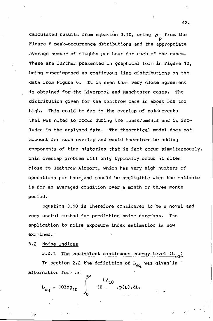
3.2.1 The equivalent continuous energy level (L ) -- eq-In section 2.2 the definition of Leq was given~in '
alternative form as 00
LilO Leq = 1010g10 1
o 10- _ .p(L) .dL.
"

43.
where p(L) is the probability density func.tion of the time
distribution of level L. Using the A and peA) notation of
the preceding subsection (3.1), the form of Leq can be
rewritten as
cb ).
1 Yl0 Leq = 1010910 10 .p().) .d>'
,0109,0 [0 ";10 dp (A) = dA .d .x 0.11)
From equation 3.10, with K.= 6.2S(a/n )xl03, we obtain
where Z ,;
Equation 3.11 therefore becomes,
L eq = 1010g [ ~. 10 {"'l K,
This can be expanded to,
B where cL = 10
J\
LSO
1010
(3.12)
-cO -§ '!£
f 10·Z
• 10 (1 + erfZ)dZ]
+00
_00
( ~Z 10109
10j 10 (l+erfz)dz
+00
..... (3.13)
The last term in the above equation has been numerically
evaluated for various levels of op in the range
3 L.a- L 16 (dB) p

and the results graphically presented in F!gure 13. So
L can now be estimated by means of equation 3.13 and eq
44.
Figure 13. An approximation to the last term is also shown
in the Figure. This has been restrained to a single c- 2 p
term for the following purpose:
With the last term approximated by 0-2/10, (which is p
within +ldB over the range 61: er!: 15, and underestimates - p
at lower o-p> equation 3.13 becomes,
A 0;:;2 ~ Leq = L50 + ~ + 10109 10 ({<f ) - 1010910 K,
" = L 50
• • • •• (3.14)
Using again the assumption of a Gaussian distribution of
peak level occurrences, then the average peak-energy level
is, " op2
L = L50 + 8.68 (from equation 2.7).
Also, we have
K,= 1010910 (6.25 ~ 103
x U) 1010 910 x n
Equation 3.4 therefore becomes,
2 - up /65.8 - 29.5, dB (3.15)
This can be compared with the Noise and Number Index and Com
posite Noise Rating when these are written in terms of the
average hourly number of events; thus,
~: ' ,;
, , _.

NNI = L + 1510g10n - 63.8,
CNR = L + 1010910nf + 1.8,
PNdB
PNdB -.
45. (3.16)
(3.17)
where the NNI is a 12-hour index and CNR a 24-hour index.
If ~ equal to between 6PNdB and 7PNdB is taken as p
typical and a site is considered where h is typically
915 metres (3000ft.) slant range, U is typically
91.5metres per second (300f.p.s., 190 kts), then the Leq c
formula becomes,
PNdB (3.18)
The apparent differences among these index forms must
be resolved by their correlation to attitude survey data.
However, if a very wide range of uncorrelated noise and
number conditions were included in the survey then it must
be expected that only one of these index forms would emerge
as most suitable.
Calculated values of Leq and NNI, using equations 3.15
and 3.16 are given in Table V for the Heathrow, Manchester
and Liverpool site conditions. These are plotted in
Figure 14 and suggest the co-relationship
L = 0.80NNI + 44.5 (PNdB) eq
While this agrees with other empirically derived relation-
ships for converting NNI t? Leq , a comparison of Equations
3.15 and 3.16 would suggest that a more accurate expression
is,
= NNI - 510g10n +
+ 1010910(h/l000)
34.3
- 1010g(U/100) 2
-~ 65.8 (3.19)
______________________________________________________________ "1

46.
Average values of speed (U) and altitude as functions
of distance along route (from start of roll) are derived
in Section 5 for application to the noise prediction
method.
Referring back to the discussion in Section 2.2.2 of
the difficulties associated with tre application of Leq to
aircraft noise exposures, it can be seen that the fore-
going analytical work has helped to resolve these. A
detailed knowledge of the noise duration distribution can be
obtained from available information on the peak level occur-
rences. The dependence of L on traffic and other paraeq
meters can be more readily appraised and various trade-off
approaches to reducing an L assessment can be derived by eq
means of equation 3.15.
3.2.2 The Noise Pollution Level (LNPl
The LNP was conceived by Robinson of the National
Physical Laboratory as being of the form,
where ~ can now be regarded as the standard deviation of
the noise duratbn distribution. When applied in a regres
sion analysis of Griffiths and Langdon's road traffic survey
data (Reference 8) the form of LNP was found to be,
which for a Normal (Gaussian) distribution of noise durat-
ions gives ~ = 2.56. That is,
which i~ now the known form of LNp •
. ,.

47.
So, to estimate LNP by measurement ~r predictive
methods, there is again the need to develop the noise durat-
10n distribution. This time it is not only for an evaluation
of Leq but also for a:L. No attempt is made here to derive
a simple equation for CL in terms of the peak-occurrence
and traffic statistics. The obvious available approach,
using the results of the earlier sections, is to evaluate
both Leq , o-L and subsequently LNP by develop~ent ~nd
analysis of the duration distribution. For a single site
assessment, this can be done quite quickly by manual comp-
utation. Fora large number of sites recourse can be made
to a fairly simple digital computer programming task.
Before leaving t~e LNP as a discussion topic, an
interesting point can be made regarding its formulation.
It has been shown in Figures 5 and 6 that for aircraft noise
exposures the peak-occurrence and noise duration distribut-
ions are well separated in their significant level range A A
(as indicated by Ll -Ll , Ll0-Ll0 , etc.). The standard dev-
iations of the distributions, c-p and c-L respectively,
are also quite different for any particular site, but this
difference decreases as the average number of flights per
hour is increased. Now reference to Figure 15 and equation
3.10 provides an interesting comparison for road traffic
noise. The Figure contains analysed data for peak distribut
ions and noise duration distributions o~ned from tape
recordings of noise exposures near the M6 motorway. The
measurement site was 36.5 metres (120ft.) from the motorway
and the traffic flow rate was 1100 vehicles per hour •
. ,. . ~

48.
(The actual sample time was 15 minutes). Taking the aver
age vehicle speed as 100km/hr. (60m.p.h. or 88f.p.s.) and
observing that a-p is about 7dB, Equation 3.10 gives for A
LSO - LSO '
which agrees with the measured data despite the obvious
question of overlap error. Purther examination of equation
3.10 and change of the propagation exponent from 2.67
(8dB/distance doubling) for the road traffic case, gives
the inequal ity,
AL L ~ 4 5 103(~) 50 - 50" • x n
So, at distances of about 20 metres from a very busy city A.
road the separation between LSO and LSO would be expected
to be very small. This closeness of the peak and noise
duration statistics has apparently been observed in measured
L10 data, as use is sometimes made of a method of measuring
L10 by reference to the peak needle fluctuations of a sound
Level Meter.
With this point made, regarding the near coincidence
of the peak and duration distributions for road traffic
noise, some inference can be made about noise indices.
Por the coincidence case,
L = Leq , crp = or. and LNP = L + Kop
. With the addition of a number term this would look very
\

49.
much like a Noise and Number Index for road traffic. The
crp term would be an additional accounting of the traffic
mix condition and hence of the variability of the noire
that Robinson suggests should be included.
3.3 Summary
In this section an analytical noise model has been
developed which allows the distribution of noise excursion
durations to be predicted from knowledge of the more stable
peak statistics and other parameters. ~t has been shown
to give good agreement with measured data and to provide
a simple means of predicting Leq and LNp •
It uses as a predictive tool is of course dependent on
the availability of a separate method for predicting the
peak-level distribution for air traffic. Many predictive
methods capable of satisfying this latter requirement are
currently being used for NNI assessment purposes although
their usage is usually restricted to estimating Land
15logN directly. The basic form of these methods is dis
cussed in ttenext section and an alternative method is
derived from further study of the Heathrow site noise
measurements.

50.
4.0 THE PREDICTION OF AIRCRAFT NOISE PEAK LEVELS
4.1 Introductory Review
The noise radiated outwards from an aircraft to a dis-
tant site is a complex mixture of frequency spectrum compon-
ents emitted from various stages of the aircraft engines.
The components may be tonal, such as the whine of the engine
compressor or fan, or may be broadband random such as the
roar of the jet efflux noise. They may be predominant in a
particular frequency region of the auditory spectrum range,
or extend over a wide spectral domain. From a noise exposure
prediction viewpoint, the contributory sources are of little
interest because their individual contributions are difficult
to estimate even when detailed inform'ation on the engine
operating parameters is known. Of greater significance is
the influence that the spectrum shape and content plays in
controlling the behaviour of the subjective aspects of the
noise, as summarized by the PNdB level or other noise scales.
Many studies of these spectral properties have been per
formed (References 2,3,4,32,33,34 for example) with various
purposes in mind. Some of these have led to well-developed
empirical methods for the prediction of aircraft noise levels
(References 24 to 26 for example). Such results are used
here, in conjunction with other data, to derive a peak level
prediction method suited to estimating noise exposure
statistics.
The flight path of an aircraft using an airport can be
partially defined by the ground trace of its allocated arrival
or-departure routeing. In following this routeing the aircraft - .
will be operated at different engine-power settings to pro-
: ,

51.
vide the necessary climb rate or descent-rate commensurate
with performance and safety requirements. As the noise
output from the aircraft varies with engine power setting,
so also does the height profile of the flight path, thereby
causing a double influence on the noise level reaching the
exposure site. The prediction of the noise peak level due
to an aircraft event must therefore be based on an -adequate
modelling of the power-setting profile of the aircraft flight
path. This is commonly achieved by defining the operation
as a segmented history of power-setting modes, comprising
the appropriate of the following settings:
(i) ma'ximum take-off power
(ii) noise-abatement climb power
(iii) climb-to-cruise-level power
(i v) 3-degree glide approach power,
Other settings, such as reverse thrust after touch-down
and level flight to intersect the glide slope, can be
included in the noise model.
A typical take-off procedure from airports where noise
abatement procedures are mandatory will consist of a maximum
power take-of~ from the runway "to a height of at least
1000ft., at which power will be reduced to a setting which
provides a reducing level of noise at ground level while
maintaining a minimum climb rate of 500ft. per minute."
This cut-back power condition is usually maintained to-a
height of at least 3000ft. (or 1000metres) and is followed
by an increase of power setting to give an increased climb-
,
.'

52.
rate to achieve cruise level, or to give_increased flight
speed. Local airport traffic controls may dictate other
procedures, such as level flight at 2500ft., when crossing
navigational beacons.
For noise prediction purposes, when account must be
taken of flights by different aircraft on different routes,
the most common approach used is to categorise these
events. For each event category a model of the flight
path profile and aircraft noise emission is compiled.
Figure 16 shows a straight-line-segmented representation
of a flight path travelled by an aircraft in its departure
from an airport. For digital computing purposes this
flight path can be represented by a system of ground plane
co-ordinates, two co-ordinate values being used to specify
the extremity of each segment of the~ojected ground
trace. The height profile is initially defined by the
ground run distance and maximum climb rate. The model is
further segmented to include subsequent changes of aircraft
power setting, giving changes in the climb rate and in the
noise output from the aircraft. Thus the noise output is
constant along a segment, but may differ from segment to
segment.
The noise exposure at any site in the'vicinity of the
airport can, in general terms, be defined by the peak noise
level caused at the site by each aircraft and by the durat
ions of the noise above specified levels. For the flight
trajectory shown in Figure 16 it is therefore necessary
to estimate the maximum radiated noise level at-the site
,

53.
and the duration of the noise excursion above the specified
levels. In a computerised method this can be accomplished
for each segment of the flight path, the peak level for
the overall event being the highest of the segment maxima
and the total durations being summated over the segments.
This approach is repeated for other aircraft using the
route and for other conditions of climb rates and power
settings along the route and subsequently for all other
routes and route users which contribute to the site noise
exposure. From the resultant set of peak noise levels,
the average peak energy level and the number of events above
various specified levels can be computed, leading to an
NNI estimate and to the peak distribution. The total
noise durations above preset levels (e.g. BO,B5,90,95PNdB,
etc.) can be used to give estimates of Ll0,L50,Leq,LNP'
etc., for each site. By continuing this computation pro
cess for a grid-matrix of site co-ordinates and using an
interpolative sub~outine on the results, iso-noise contours
can be plotted for the airport region in any of the esti-
mated exposure parameters or indices.
This computational method is essentially similar to
those used in the U.K. and U.S.A. for NNI and NEF predict
ions. The particular form described above and developed for
noise duration estimates is reported in Reference 35. One
of the limitations of the method is that of adequately des
cribing the variability of the noise peak levels at a site,
particularly when most of the flights have a common route
and height profil~. The method also requires a very elab-

54.
orate and detailed analysis of the airport traffic in terms
of destination range, which indicates the climb-rate capa
bility of each aircraft. These problems could be overcome
by a less rigorous breakdown of the climb-rate dependency
than that given in Table 11 and by incorporating a lateral
s~ad of the aircraft routes about their defined (Figure 3)
traces.
An alternative approach is pursued in the present
study. This leads to a simpler method of predicting the
peak level distribution for a site, which can then be used
in conjunction with the Section 3 results to give estimates
of other noise exposure properties. It is based on measured
distributions of noise peak levels, rather than on elaborate
distribution of the climb profiles of aircraft flights
along a route. From a practical viewpoint, the former is
more readily measurable and in the earlier discussions was
considered to be stable such that a measured distribution of
peaks can be taken as a long-term characteristic of a site
exposure.
4.2 An Alternative Method
Figure 17 shows a breakdown of the noise peak data for
each of a number of aircraft groups which contributed to the
total peak level distribution at two sites near Heathrow.
The total peak distributions are taken from Figure 5 and
were measured at the two sites shown in the insert, one
being subjected only to aircraft landing movements and the
other only to take-off events. The noise peak data for
individual aircraft and aircraft groupings were compiled
" . ,.

55.
by cross-reference of the measured event peaks with the
actual runway utilization logs for the measurement period.
In the take-off data, only aircraft using Clacton/Daventry
departure routes have been extracted from the overall
compilations.
The landing case data are of special significance
because the aircraft flights are constrained to two well
defined approach paths, the 3-degree 'glide-slopes' for
each runway. No obvious deviation from the nearer of these
paths was observed for the runway 28R landings during the
test period. Although the mean peak levels of the aircraft
group data are well spaced discrete values, the dispersion
of the peaks about these mean values is sufficient to trans
form the total distribution into a continuous form. A more
detailed presentation of these data is given in Table VII
which shows that breakdown of the noise peaks by aircraft
type, rather than by grouping, provides very little reduction
of the dispersion. The typical standard deviation of the
data is about 3.5dB for an aircraft type or grouping.
The departure case data of Figure 17 are similarly
dispersed in each aircraft grouping, the typical standard
deviation being of the order of 5dB. Again, breakdown by
aircraft type provides little benefit (Table VIII). In
these cases there are explanations for the noise dispersion,
other than that of a variation in engine power settings,
which have been described as lateral and vertical flight
path spreads. Horonjeff and Soroka (Reference 36) attempted
an analysis of these spreads by reference to histograms
, ,
, ,
t
56.
of take-off weights, but the latter could not be found to
follow any established probability law.
The alternative approach to predicting noise peak dis
tributions is based on the observations of the peak level
dispersion. It is assumed that the air traffic along a
known approach or departure route can be described by a
categorised breakdown of the traffic mix, namely:
Jumbo (B747)
4-engined Turbofan (B707, DCB, VC10, etc.)
3-engined Turbofan (B727, HS2l, etc.)
2-engined Turbofan (OC9, B737, BAC1-ll, etc.)
4-engined Turboprop (VC8, VC9, etc.)
Other categories, such as wide-body, 3-engined aircraft
(OC10, L10l1) or 2-engine turbopropellor aircraft can be
included when necessary.
Now rather than account for the noise distribution by
further subdivision of the traffic mix, as is required for
use of Figure 4 via Table 11, we can associate the mean
peak level caused by each aircraft category with the mean
flight profile for that category. The dispersion of these
peaks about their respective mean values can be subsequently
made in the statistical development of the noise distribution.
To predict the mean peak level caused by each air
craft category it is necessary to know the slant range dis
tance of the (average) flight path relative to the exposed
site. The horizontal component of this distance can be
taken as the minimum distance between the site and the
defined ground trace of the intended route (Figure 3).

57.
The vertical component (height) can be o~tained by con
structing ?n average climb profile for the particular air
craft category. An example of this is now developed.
From tables of "Aircraft Type and Utilization" pub
lished in the Civil Aviation Authority Monthly Statistics
(Reference 37) the average stage destination range of each
of about thirty different aircraft types used as U.K.
airports can be calculated. Taking summer season statistics
and calculating these averages for the type-categories
mentioned earlier, the typical stage distances are,
B747 3900 miles
4eng.TF 3200 miles
3eng.TF 700 miles
2eng.TF 600 miles
These values can be used in conjunction with Figure 4 and
Table 11 to define the average initial take-off profile
of each aircraft category. The subsequent profile character
istics are dependent on the power cut-back climb rates and
where these commence. For the Reference 35 computer
programme, the present author used a cut-back rate given
by 40% of the initial climb-rate, and a cut-back point of
5.3 kilometres from start of ground run (provided the air
craft height exceeded 1000ft.). Comparison of the profiles
given by these procedures, with radar-tracked height data
provided by the Civil Aviation Authority, is shown in
Figure 18. It is seen that the profiles would agree slightly
better if a cut-back commencement criterion of 1500ft.
height was used. It is also evident that there is no
,> •• '

58.
noticeable change in climb rate at the 3000ft. height
point.
Figure 19 shows the developed average height profiles
for the five aircraft categories, based on the preceding
arguments and observations. These can be used to develop
the peak level distributions of noise for any site and
for the noise duration computations of Section 3 (by
calculation of the slant range distances). The landing
path height profiles are simply given by a 3-degree glide
slope extending from a runway point that gives 50ft.
clearance height at the runway threshold, to a height of
2000ft. which is the usual intersection from a level flight
approach condition.
The remainder of the peak distribution development
is fairly straight forward. The mean peak level caused
by each of these aircraft categories and its flight pro
file is estimated by means of any preferred method ,
(e.g. References 24 - 26). One method is given in the
next sUbsection. These are inserted in Column 2 of
Table IX. The percentage fleet mix of the aircraft using
the route is inserted in Column 3 of the Table. These
route-usage percentages are now distributed over the 5dB'
incremented (peak) noise level bands as follows:
Band containing PL2
Bands containing PL2 - 5dB
and PL2 + 5dB
Bands containing PL2 and PL2 + 10dB
10dB
O.38P%
O.24P%, each
O.07P%, each
, , ;

These are derived from standard deviations of aircraft
noise in take-off conditions. For aircraft on approach
routes the corresponding criteria are:
PL2 Band O.GOP');
59.
PL2-5dB and PL2+5dB Bands
PL2-10dB and PL2+10dB Bands
0.19P%, each
O.OlP%, each
With the appropriate percentage occurrence values
inserted in the Table, the cumulative distrib~tion can be
obtained by column summations. The probability of peaks
exceeding each 5dB incremented level is then obtained by
right-to-left cumulative summation of the column sums.
The description given above applies only to the
traffic on a single route. This can be extended to apply
to traffic on a number of routes, provided the Column 3
summation total is 100%. However if noise durations are
to be estimated it is essential that the different routes
be treated separately.
4.3 Aircraft Noise Peak Levels
The modelling of the noise of an aircraft is most
readily accomplished by definition of a noise level at a
specified reference radius from the aircraft, together
with a propagation law for the estimation of levels at
other radii. Since such modelling is, of necessity,
empirical in derivation then the precaution must be taken
that the reference level and propagation law are compatible
over a wide range-of radii, thereby providing minimised
error over the range rather than at one radius only. Thus
the reference value must be derived in conjunction with
. " , .

60.
the propagation law. The model can be expressed as:
where Lij(R) is the noise level produced by aircraft type i
at power setting j, at the reference radius R; Lij is the
corresponding level at some other radius r; and Aij(r,R)
is the atmospheric propagation loss over the radius differ-
ence between rand R.' For peak noise levels it is the
common practise to base the model on the minimum slant
range distance between the site and the flight path (segment).
The model is therefore of cylindrical radiation form, as
opposed to a spherical form and the expression required is
(4.2)
In order to use, and compare, reference data from other
literature, the reference sideline distance R'is taken
here as 1000ft. (304 metres).
The propagation law can be expressed in many different
forms; as a constant attenuation per doubling of distance,
or as an attenuation per unit distance, or as a combination
of these. The last is probably the most accurate as the
attenuation. has a spherical divergence content (6dB per dis-. " ~
tance doubling) and atmospheric losses (dispersion and
dissipation) which are usually expressed as ~er unit distance.
However, for extrapolation of noise levels in PNdB units
the use of a distance doubling law has become the most
common approach. With this, the value of BPNdB per distance
doubling can be taken for air-to-ground propagation (that
is, for propagation paths at high incidence angles to the
ground plane) without much controversy. Lanzer's peak

61.
level data (Reference 32) suggests that attenuations of
the order of 10 or 11dB(D) per distance doubling are more
accurate for the maximum power take-off condition.
De Witt's limited data (Reference 38) also suggests this
and that the 8dB/dist. doubling occurs at cut-back power
condition. However, without extensive sUbstantiation
that these results apply to peak PNdB levels over a wide
range of distance, there seems little justification (at
present) for use of these higher attenuation rates.
Equation 4.2 therefore becomes, for air-to-ground propa-
= (4.3)
where r is in metres. (R = 304 metres).
Application of this propagation law to available pub-
lished data on noise peak levels allows a comparison to be
made of the reference levels suggested by these data.
These are compiled in Table X for the landing, level
flight, and take-off modes of aircraft operation. The set
of reference peak levels to be used in the following sec-
tions is also given in the Table.
4.4 Noise Propagation at Low Ground Angles
Equation 4.3 must not be used for the prediction of
noise level at sites where the propagation path is at low
angles to the ground plane (less than 15 degrees, say).
For such cases the extra attenuation caused by ground-
effect dispersion and dissipation can be very significant.
This excess (relative to the air-to-ground attenuation)
is very much frequency-dependent and will of course vary
J'

according to the nature of the ground cov~rage (grass,
woodland, residential area, etc.). Figure 20 shows same
62.
published data on the form of the ground effect. In
Figures 20(a) and (b) it is presented as an attenuation
per 1000ft., whereas in Figures 20(c) it neither conforms
to a constant value per unit distance nor a constant value
per distance doubling. This latter point is also true of
atmospheric effects, but when these are applied to the
frequency spectra of aircraft noise, and the result evaluated
in PNdB units, the 8PNdB per distance doubling law gives a
reasonable approximation to the total loss. (The law was
actually derived from measured PNdB data). A similar simple
law for ground effects on aircraft noise propagation is
therefore expected. Discussions with other agencies who
work on aircraft noise predictions reveals that there is some
disparity in the laws used and in the derivative basis of
these laws. The subject is therefore examined here to pro-,
vide a reasonable basis for the adoption of some law that
can be used in the present work.
First, an examination of Table XI gives a direct com
parison of some simple attenuation laws that could be used
for the total losses (including the air-to-ground term). It
is seen that thee logarithmic forms (constant attenuation per
distance doubling) approximate closely to the combined logar
ithmic and linear-forms over a range of distance. The
following points should also be noted:
- , ~.

63.
(i) It is well known that the application of a linear
attenuation 'law to the overall level of a complex
frequency spectrum noise gives a gross underesti
mate of the level expected at large distances.
(This is due to the continuous change in frequency
component significance that occurs in reality.)
(ii) For airport noise exposures there is no need to
predict very low noise level values. For NNI
assessments 80PNdB is the limit of interest. How-
ever, taking 70PNdB as a more general limit of
interest, the maximum attenuation range is of the
order of SOPNdB (re. the 1000ft. range levels).
(iii) If the need was to predict mapped contours of
iso-noise level, then the various models in Table
XI would give considerably different spreadings
of these contours.
Now taking these points into account, Table XI can be used
to assess two particular propagation laws that have been
used 'for noise exposure estimation purposes. These are,
10PNdB per distance doubling, and
lSPNdB per distance doubling,
for ground-to-ground radiated aircraft noise. The first
corresponds to an average ground excess attenuation of
1PNdB per 1000ft. up to a range of about 8000ft. (2.4km)
and a lower attenuation thereafter. This does not compare
well with the Figure 20(c) aircraft noise data, which were

64.
measured under the more favourable propagation conditions
of a "down-wind" greater than 5 metres per second. On the
other hand; the 15PNdB per distance doubling corresponds
to an attenuation of 3.5PNdB per 1000ft. to a range of ,
4000ft. to 8000ft. (2.4km), and lPNdB/l000ft. from 8000ft.
to 16000ft. (4.88km). While this might seem to be conserv
ative in the light of the Figures 20(a) and (b) data, and
possibly reasonable in consideration of the downwind
effects on the Figure 20(c) data, there is obviously a need
for some experimental justification of such a high attenu-
ation rate. A limited attempt at such justification has
been included in the present work, by the inclusion of two
other measurement sites in the Heathrow noise survey
(Appendix I). These sites were located at Hanworth Park
and Kempton Park Race Course, to the south-east of
Heathrow Airport runways. The distances to the (approxi
mate) start-of-run point of Runway 28L are about 4.5km
(14,800ft.) and 6km (19,700ft.) respectively. Analysis
of the recorded data has yielded useful noise level data
from the 4.5km site measurements, but none such from the
6km site. The problem in the latter case was that of dis
tinguishing the take-off ground run noise events from
other noise events in the background.
The 4.5km site data have been analysed in dB(D) units,
and the peak levels for the ground run portion of-the
noise histories are given in Table XII. The mean peak level
and the standard deviation of'the peaKS is also given in
the ~able, for each aircraft category. A comparison of
! ':

65.
these mean values with the reference levels (for 1000ft.
range) of Table X, allowing dB(D) equal to PNdB minus 7dB,
gives an average attenuation of 48dB(D). This corresponds
to an attenuation rate of,
12.3dB(D) per distance doubling
over the 4.5km (14,600 ft.) range and for peak noise levels
of the order of 60 to 70 "PNdB" at this range.
With this attenuation rate the peak levels at the 6km
distant site would be expected to be 5dB lower, but this
could not be verified because of the inability to separately
identify the aircraft ground run noise excursions from
other excursions of the expected magnitude.
This 12.3dB per distance doubling rate cannot be
readily applied to the estimation of PNdB levels without
some check on the relationship between dB(D) and PNdB in
these near-ground propagation conditions. Rather than
analyse all of the data for their peak PNdB levels, a sample
of BAC 1-11 and DC-8 aircraft recordings was selected for
this more detailed analysis. It was found that the difference
between PNdB and dB(D) unit levels for the noise peaks was
typically of the order of 5dB. Using this in the comparison
with the reference data gives an attenuation rate of,
12.8PNdB per distance doubling
for ground-to-ground propagation.
Without further derivation or justification, this
rate is taken here to be appropriate to the zero ground

66.
incidence attenuationcr aircraft peak noi~e levels. A
smooth continuous reduction of th~rate for ground angles
increasing to 15 degrees (at and above which the 8PNdB per
distance doubling law is used) is given by;
•••••.•••• (4.4)
where r is in metres, and Q is the propagation grazing
angle relative to the ground plane.
This is shown graphically in Figure 21.
, '\

67.
5.0 NOISE EXPOSURE PREDICTION BY A GRAPHICAL METHOD
The methods developed in Sections 3 and 4 are amenable
to a simple chart-form presentation. These are summarised
in the following two-phase analysis description. The dis
tribution of noise peak levels is developed first and from
this the noise duration statistics are evaluated. An
example of method's application is given in Appendix IV.
The information required is as follows:
(1) the distance along the route (ground trace) from
the usual start-of-run position on the rum~ay to
the nearest point of,approach to the noise
exposed site;
(2) the side-line distance from the site to this
closest point on the ground trace;
(3) the typical percentage fleet-mix of the aircraft
using the route, defined in categories
Jumbo-jet (B747)
4-engined turbofan
3-engined turbofan
2-engined turbofan
4-engined turbopropeller.
, (2-engined turboprop and 4-engined piston aircrart
can be included as a separate combined category.)
(4) the average hourly number of flights using the
route. This number should include only those air-
craft that fall into the item (3) categories.
The average should be for the specific period of
the day that is required for an index evaluation,

68. (e:g. between 0600 and 1800hrs. GMT for an NNI
estimate.) It should also be the average for any
specified long-term period required in the index
definition (e.g. for a 3-month summer period NNI).
5.1 The Noise Peak Level Distribution
The peak-level distribution is developed as follows:
(a) From Figure 22 or 23 obtain for each aircraft
category the mean peak level, PL1 , by reference
to the distance along the route to the nearest
point of approach (item 1).
(Figure 22 has been derived by direct combined
use of the Figure 19 height profiles, the Table X
reference peak levels and the Figure 21 attenuat
ion rate for very large angles.)
(b) From Figure 24 or 25 obtain the corrections (ALl)
for side-line distance, applicable to each air
craft category.
(c) Calculate the mean peak levels caused at the site
by each aircraft category,
PL2 = PL1 -ALl
and insert these in Column 2 of Table IX.
(d) Insert in Table IX, Column 3, the percentage usage
of the route by each aircraft category.
(e) Distribute the percentage route-usage values over
columns 4 to 11 according to the procedure des
cribed in Section 4.2. That is,
'I

Departure Routes
Band containing PL2
PL2-SdB and PL2+SdB bands
PL2-10dB and PL2+10dB bands
Approach Routes
Band containing EL2
PL2 -SdB and PL2+SdB bands
PL2-10dB and PL2+10dB bands
O.38P%
O.24P%
O.07P%
O.60P%
0.19P%
O.OlP%
69.
(f) Calculate column totals, which are the percentage
number of peaks occuring in each SdB band. Calcu
late right-to-left cumulative totals. These are
the percentage of peak levels exceeding each noise
band lower limit.
(9) The percentage exceedence values should be plotted
on a Normal Distribution Probability chart as shown
in the Figure Sand 6 examples. The best fit
straight line should be drawn through these data
points, and the upper (truncation) limit of the
highest-occuring noise band should be marked on the
line.
This procedure gives the level-exceedence distribution of
the peak noise level occurrences.
S.2 The Noise Duration Distribution
The level-exceedence distribution of noise durations
is obtained by means of equation 3.10 (of Section 3.1),
with allowance for a different noise propagation exponent.
A step-by-step procedure for applying this equation is as
"
, "
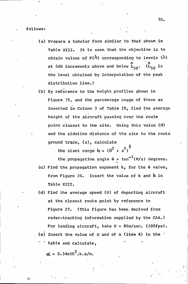
,
70.
follows:
(a) Prepare a tabular form similar to that shown in
Table XIII. It is seen that the objective is to
obtain values of P(~) corresponding to levels (~) A
at SdB increments above and below LSO. '" (LSO is
the level obtained by interpolation of the peak
distribution line.) ,
(b) By reference to the height profiles shown in
Figure 19, and the percentage usage of these as .
inserted in Column 3 of Table IX, find the average
height of the aircraft passing over the route
point closest to the site. Using this value (H)
and the sideline distance of the site to the route
ground trace, (s), calculate 2 2 t
the slant range b = (~ + S )
the propagation angle 0 = tan-1 (H/s) degrees.
(c) Find the propagation exponent k, for the 0 value,
from Figure 26. Insert the value of k and h in
Table XIII.
(d) Find the average speed (U) of departing aircraft
at the closest route point by reference to
Figure 27. (This figure has been derived from
radar-tracking information supplied by the CAA.)
For landing aircraft, take U = 86m/sec. (280fps).
(e) Insert the value of U and of n (item 4) in the "
table and calculate,
3 cL = 2.34x10 .k.a/n.
. .

71.
(f) From the developed peak level distribution obtain
a value for OJP' by,
" " ap = (L10 - LSO )/1.2S. !
(g) From Figure 2a, obtain values of Bquation 10 right-
hand-side (RHS) corresponding to the calculated 1\
(Jp and each value of (LSO -A) shown in the
Table XIII. Insert these in the Table and calcu-
late each peA) given by
peA) = RHS/o(.
(h) Plot these peA) values on the chart used for the peak
distribution. In each case the level ~ dB is 1\
given,by its ~ncrement relative to LSO· The level
exceedence distribution of noise durations is thereby
obtained. This corresponds to the distributions
shown in Figures 5 and 6.
5.3 Noise Indices
The Noise and Number Index (NNO can be evaluated by
means of the peak-level distribution, and equation 3.16.
That is,
NNI = Lao + lSl0910naO - 63.S, PNdB
where naO is the number of events exceeding aOPNdB (per
hour) and Lao is the average peak-energy level of these
events.
The percentage of peaks exceeding aOPNdB is read directly
from the developed peak distribution. The product of this
and the total number of flights Cn, item 4) gives naO as an
average hourly value. The value-of LSO can be obtained by
graphical integration of the peak distribution between the
limits of SOPNdB and the upper truncation level. This is " ....
d

described in secti~n 2.2, Equation 2.9. ~lternatively,
the expression
L =
2 0p 8.68
72.
can be used provided account is taken of the limits (see
Appendix Ill).
The Equivalent Continuous Energy Level (Leq) is
obtained from Equation 3.14 by use of the peak-level dis-
tribution, or from Equation 2.9 which is an integration
of the noise duration distribution. An example of both
methods is presented in Appendix IV. Use of the approximation
for a Gaussian distribution is not recommended.
Other Noise Exposure Parameters, such as L1 , L10 , LSO '
etc., can be obtained directly by interpolation of the
developed distribution. The standard deviation of the noise
level excursions (~) can be easily obtained for a Gaussian
distribution. For non-Gaussian data recourse must be made
to statisttal analysis of the variance about the LSO level.
This can be performed by use of the plotted distribution.
With Leq and ~ known, the Noise Pollution Level (LNP
) can
be obtained.
Note that, whereas L values for different routes eq can be energy-added to give a total exposure Leq , other
indices cannot be so treated.
The overall average peak energy level (LT) caused by

73.
operations on two traffic routes can be obtained from the
individual route L1 and L2 levels as follows; '[; -
LT = 1010g1~ [ n1;n
2 ( n110 1/10 + n210L2/10 )]
where n1 and n2 are the respective route usage numbers
(exceeding 80PNdB).
The NNI becomes
Finally, it must be remembered that the graphical represent
ations of the mean peak levels (Figures 22 and 23) and the
sideline correction terms (Figures 24 and 25) are based on
specific models of height profile. These were derived from
destination range estimates averaged over U.K. airports.
For any particular airport it would be preferable to
rederive the charts fur the aircraft operating out of that
airport. Account should also be taken of any height
restrictions imposed on flights along any route.

-- - ---------------------
74.
6.0 MEASUREMENT AND MONITORING CONSIDERATIONS
In the preceding sections attention has been given
almost exclusively to the problems of estimation by pre
dictive techniques. An equally essential aspect of noise
assessment is that of noise measurement and monitoring, which
may take the form of intermittent sampling, occasional
precision measurements over a single day or period, or
long-term, continuous recording and analysis. It is clear
that long-term measurement exercises are more of a research
tool than an assessment approach and that noise contours
based on three-month averaged estimates are more readily
obtained by the predictive techniques. The need for mea
sured data will persist however, especially for specific
site assessments and for verification of predictive methods
and results. Some guideline suggestions have arisen in the
preceding sections as to methods by which data should be
acquired for such purposes. The present section is a brief
summary of these guidelines.
First consideration must be given to the objectives of
a measurement task. For an estimate of NNI or other peak-
level based exposure index it is recommended that the peak
level data be acquired and stored in a manner that will allow
the statistical distribution of maxima to be developed.
Where there is a possible need, or future requirement, for
evaluation of duration-based exposure measures such as L10
or Leq then it is recommended that data be acquired on both
peak and level-exceedence distribution statistics,
simul t;aneousl y •.
The use of D or N-weighted sound level, with appropriate -<-'\
, ,

75.
correlations, is considered to be an acceptable measurement
alternative to PNL measurement for purposes of cumulative
noise exposure assessment. This allows great simplification
of the noise measurement and ana~is tasks, particularly
as on-line monitoring of the data can be accomplished with
relatively uncomplicated instrumentation. The correc.tions
for near-ground propagated noise need to be studied in
some detail, however.
The measurement task should employ "precj.sion-grade"
instrumentation. Careful consideration should be given to
the selection of the measurement transducer (microphone),
particularly to the directional characteristics of the unit
when noise duration estimates are required. In the field
exercises reported here, the transducers were free-field
response units. A preferable system is a pressure-response
unit, mounted in a grazing-incidence orientation with
respect to the flight path. Recording of the noise signal
history on magnetic tape was found to be easily practised
with a recording "switch-on" trigger at 65dB(O) for each
'event. The termination of each event-recordingWis not so
readily definable in terms of a fixed level because of
sudden drops and resurgences of the level after aircraft
pass.
Estimates of the traffic parameters n , hand r should
be recorded with the stored data, where n is the average
hourly traffic count for the period of measurement, h is
average height of the aircraft and r is the average slant
range distance.
, ,
.,

76.
, The selection of a noise-measurement period must
depend on the characteristic airport or route usage. A
continuous attendance period at a site should preferably
be 12 hours for a Noise distribution assessment. Noise
sampling methods over a number of days or weeks should
attempt to construct the distribution of noise expected in
a single day period, whether worst case or averaged, and it
is here that much of the difficulty will arise. Particular
attention should be given to Ca) the variability of aircraft
movement numbers on a day-to-day basis, Cb) whether rum~ay
usage is shared on a preferential system or, for multiple
runway airports, whether the sharing of runway usage is
based on a consistent, time-period, allocation, and Cc) the
hourly characteristics of the movement schedules.
Finally, it can be claimed that one of the greatest
problems is knowing just' how elaborate a measurement tech
nique should be to satisfy the requirements of the noise
assessment exercise, or in other words, "what price should
be paid for accuracy?" Are digital computer facilities
and highly-expensive measurement equipment really necessary
for the purpose of estimating a noise index which, in
itself, is criticized as being inadequate? The answers
to these questions must depend on the immediate application
of the estimate. For compensatory purposes an erroneous
estimate may be much more expensive than the equipment
costs needed for an accurate measurement. As a planning
guideline, however, a relaxed accuracy may be quite accept
able. In many noise exposure situations, the measurement
of an index value is not a practical proposition because
77.
of the variability of the noise from day to day and over
longer periods. To obtain estimates for sufficient condit-
ions to establish long-term averages or contours around an
airport would be an unacceptably expensive task, particu-
larly when this variability is considered. So, as predict-
ive techniques become more necessary for the assessment of
new or extended airports, it is much more desirable that
they are validated by application and test in e~isting, mea-
surable, airport sites.
-, . , j.

78.
7.0 CONCLUSIONS AND RECOMMENDATIONS
The work reported herein has been an examination of
methods by which aircraft noise exposure can be estimated;
emphasis has been given to predictive Methods.
Although the Noise and Number Index (NNI) is the only
cumulative noise exposure measure formally adopted in the
U.K. for aircraft noise assessments, the consideration
currently being given by national and international advisory
bodies to the introduction of a more generally applicable
index has suggested that a useful study of predictive
methods should include a capability to derive basic inform-
ation from which other measures can be evaluated. The
study has therefore commenced with a review of various
forms of cumulative exposure measures with some attention
being given to their basic properties and inter-relationships
in terms of traffic parameters.
It has been shown that, by means of a fairly simple
representation of traffic along a route, useful expres
sions can be derived for the inter-relationship of peak-
level and noise duration based exposure statistics. It has
been further shown that these relationships can be employed
in a predictive methodology which aims, first, at estimating
the statistical characteristics of the peak level occurrences
and, second, at estimating the noise duration statistics.
From these, most of the noise indices can be evaluated.
A comparison of the dependencies of the Equivalent
Continuous Energy Level, L ,and the NNI has-been made eq
by relating the former to-an expression ,which includes the
.,.

average peak-energy level as a constituent. The index
forms are, respectively,
2 - er:. /66 - 29.5,
P
63.8,
PNdB
PNdB
79.
where n is the hourly traffic count averaged over 12 hours,
U is the average traffic speed along its route and h is the
minimum slant range between site and the route. L is the
average peak-energy level as used in the NNI formulation.
For regions where the slant range is of the order of
915 metres (3000ft.) and crp is about 6PNdB, Leq becomes
22, PNdB
Any debate on the relative merits of these indices
must be by reference to their respective attributes in pre
dicting community annoyance. However, the derived forms of
Leq, given here, clarify some aspects of its applicability
to aircraft noise exposures. It is recommended that future
studies of index derivation by means of attitude-regression
empiricism should be accompanied by studies of the physical-
acoustic properties of the contender index forms.
An examination of the dependency of noise indices on
traffic patterns and route usage has illustrated some of the
basic problems of measurement and prediction. It is apparent
that most indices can' be considered to comprise a relatively
~ •• : I J-

80.
invariant term and a term which is greatly influenced by
the variability of day-to-day route (or airport) movement
numbers. Thus the estimation problem can be partially
alleviated by separate consideration of these terms.
The nobe peak level distribution and the average peak
energy level (L) can be regarded as being relatively stable
quantifiers of aircraft noise. They are thereby amenable
to short-term measurement for purposes of evaluating a
long-term averaged (3-month for example) index or of
validating a prediction method. Noise duration, or other
event-number based, constituents of a noise index are not
so amenable to short-term measurements for purposes of
obtaining long-term averaged values. These latter terms
·account for the accumulative effects of noise exposure and
are therefore essential to. the composition of an index.
It is concluded that expression of these terms as functions
of meaningful planning parameters (such as is already
included in the NNI and as has been derived for L ) is best eq
suited to the aircraft noise assessment problem. Account
for the variability of the exposure over a daytime or three
month period (as suggested by Robinson's LNP ) could be
readily represented by inclusion in the index of a maximum
to-average event number ratio (nmax/nave) or some similar
subjectively meaningful parameter. -
A noise-exposure prediction method has been developed
in this report. This is founded on a well-established and
documented methodology originally designed for Composite
Noise Rating evaluations of airport ~nvironments. Its

"
81.
adaptation to the present work is extended to provide
estimates of duration-based exposure measures such as L1 ,
L10 , Leq' In its original form, the method requires a
laborious breakdown of airport and route traffic into
categories of aircraft type,mode of operation and destinat
ion range. The definition of an aircraft movement in
terms of these categories can be accomplished for retrospect-
- ive assessments by reference to detailed airport movement
data, if available, or by a complicated cross-referencing
system employing runway movement logs and flight schedules.
This task is circumvented by the noise-prediction method
given herein, which is based on a modelling of the dispers-
ion of noise peak levels about an expected average for a
given category of aircraft on a well-defined flight path.
It is shown that this approach is amenable to simple chart
and tabular computation. The estimation of duration-based
nnise exposure parameters is obtained by means of the
relationships between peak and duration statistics as
developed in Section 3.1. It is recommended that further
detailed study and testing of the'statistical predictive
approach be initiated. The flexibility of the method in
providing compatible estimates of noise exposure, in various
index forms, would appear to satisfy a much needed require-
ment in predictive noise assessment capability.
, ~ • I
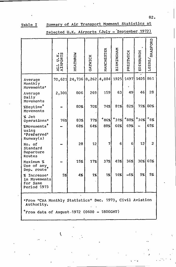
82.
Table I Summary of Air Transport M~ent Statistics at
Selected U.K. Airports (July - September 1972)
a 0:: 0
0:: :;: . r.. a .11) :;:: t.l « ~ :z: ..:
Eo< :z: u ~ 0:: ~E-< 0 ~ 11) ~ H 0: III .0:: 0:: U t.l Z :;:: ::J ......
::>0 :z: H :z: H Eo< III 11) 0. Eo< :;::
~ :;: 11) z a
....l0:: « Eo< 0:: t.l H t.l
....lH t.l « « H 0:: a t.l «..: :z: ~ :;: III 0. [iJ ....l
-Average 70,621 24,736 8,262 4,884 1925 1497 1405 861 Monthly Movements·
Average 2,300 806 269 159 63 49 46 28 Daily Movements %Daytime+ - 80% 70% 74% 81% 82% 75% 80% Movements
% Jet +86% +31% +88% +36% +6% operations· 76";. 83% 77%
+ 68% 64% 88% 66% 69% 65% %Movements - -using 'Preferred' Runway(s)
No. of - 28 12 7 6 6 12 2 Standard Departure Routes Maximum % - 15% 17% 37% 45% 36% 30% 65% Use of any+ Dep. route
% Increase· 5% 4% 1% 1% 16% -6% 9% 5% in Movements for Same Period 1973
·From "CAA Monthly Statistics" Dec. 1973, Civil Aviation Authority.
+Fro~ data of August-1972 (0600 - 1800GMT)
-
l .
\ ."

83. Table II
See Figure 4
,"

I"'" ~,
84.
'~ -
A I R POR T OP E RA T J ON S T A Ill. E - ... ",- .... - .. ~_------~---- .... -- .. - ... -------...
:-----AIRCRAFT OE3TltJATIOU ROIJTE - - - CATEGORY RAtjGE NUI1!lER
- -
POWER Pi~OF !LE
NUflnER OF EVENTS
__ M"~ ________ ~~ ___ .--_"--_______ ~ __ --------------~~ ____ ~_~.
3-7-- -,- 1 0.76 - - - -- 3 8 1 1 - 0.89
- - -4 7 ~ 1 3.40 4 8 1 1 2.32 7 4 , 1 0.03 2 5 :; 1 0.10 .3 1 3 1 0.48 3 2 3 1 0 .06 3 3 3 1 0.03 .3 8 .3 1 0.1(1 I, 1 3 1 1.94 4 7 :; 1 0.22 4 3 :; 1 0.64 4 7 3 1 0.06 4 8 3 1 0.10 ~ 1 3 1 0 . 83 --6 7 :; 1 0 • 03 8 1 3 1 0.83 8 2 3 1 0.03 1 2 4 1 0.03 3 1 l. 1 0.32 4 1 4 1 0 • 86 4 7. 4 1 0.35 4 8 4 1 C. 06 2 5 1\ 1 0.04 3 7 6 1 0.33 3 8 6 1 0.38 4 7 6 1 1 .46 4 8 (, 1 , .00 7 4 6 1 0.01 3 1 ~ 1 0.20 3 2 8 1 0.03 3 3 3 1 0.01 3 8 a , 0.04 4 1 8 1 " • 83 4 2 3 1 0.10 4 3 8 1 0.27. 4 7 8 1 0.03 4 8 i3 1 0.04 5 1 3 1 0 .. 35 6 7 i3 1 0.01
-~. ~-=~-- -- 8 1 .3 - - - ---- , 0.35 8 2 8 1 0.01
-:-, ---- 2 <) -~1 -------0.0' ---- - --'3 --.---- -- 1 -- <) .----- 1 0.14
,~~-:;~:L:-~::- 4 ' .:_--:-- ---., . ~ <) - __ 1-c~_-: -. ;,-.- 0.37-'-,._- ----- .-- - 4 - -- - -- - - 2 Q - - --,---- - --,--. 0.15
i-:~:-~;~-=-~=~'-:.:4 ~ __ - .: '.8 _ c -_ i":9~:o:_~~.: '_ -=~-1 c .--- __ -. :'0.03
.- ------.------_. ---
- I

Table IV Noise and Number Parameter Estimates for Five Sites on Various Days
-Total No. x~ - x 15logNSo NNI Date of L,Av.peak-Energy Level
Exposure of Operations Site No. Site No. Site
1 2 3 4 5 1 2 3 4 5 1 2 3
B.B.72 841 (652) 90 91 95 93 B8 4 32 35 35 15 14 43 50
10.8.72 879 (661) 93 91 95 94 B8 43 35 33 32 41 56 46 4B
23.8.72 893 (672) 93 92 94 95 89 23 35 37 33 40 36 47 51
25.8.72 f.)32 (689) 92 91 95 93 87 31 29 26 24 40 43 40 51
31.8.72 ~14 ( 702) 92 90 94 93 87 32 24 35 31 17 44 34 49
'Av. Day' ~68 - -
Aug. 1972 92 92 95 93. 89 35 32 35 33 35 47 44 50 . .
10.4.73 93 93 94 -- -- 33 32 36 -- -- 46 45 50
" (measured) 91 92 95 -- -- 31 33 36 -- -- 42 45 51 ,
,
,X in PNdB units
XXTotal No. of airport movements, including arrivals and departures, "24hr. total (12hr. daytime)".
No. 4
4B
45
4B
47
34
46
--
--
5
23
49
49
47
24
44
--~
--
00 U1 •
(
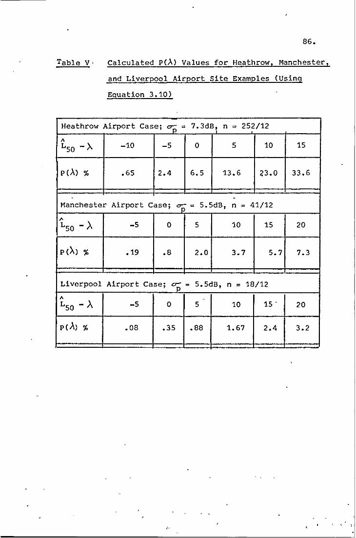
Table V,
86.
Calculated pCA) Values for Heathrow, Manchester,
and Liverpool Airport Site Examples (Using
Equation 3.10)
Heathrow Airport Case; op = 7.3dB, n i
= 252/12
" LS~ -).. -10 -5 0 5 10 15
PCA) % .65 2.4 6.5 13.6 23.0 33.6
- -Manchester Airport Case; ~= 5.5dB, n = 41/12
" L50 - A -5 0 5 10 15 20
PCA) % .19 .8 2.0 3.7 5.7 7.3
Liverpool Airport Case; op = 5.5dB, n = 18/12
" -LS~ - ).. -5 0 5 10 15 - 20
PcA) % .08 .35 .88 1.67 2.4 3.2

Table VI Comparison a Measured and Calculated NoDe Index Values for Figure 6 Sites
. Noise Measured Data NNI" L *
Airport Exposure Eqn. eq " Eqn. Site L50 op , L n/hr. 3.16 3.15 -
Heathrow 82.2 7.8 89.2 21.0 52.2 86.1 . •
E .... 0
Manchester 0 ..... 83.8 5.5 87.3 3.4 38.5 75.2 I.D ..., -I.< ID 11 <0 0'
Vl s:; Q, ID t:
Liverpool E > III 80.5 5.5 84.0 1.5 29.8 68.4 0 <: I.< I.< , .... "!:!
- ~ t: III ::l .....
Units: en 0:: III db(D) dB(D) dB(D) PNdB PNdB
*7dB has been added to convert the values from dB(D) to PNdB
,-
L * eq Measured
87.2
74.5
68.3
PNdB ,
Cl) -J •

Table VII Statistical Summary of Aircraft Type and
Grouped Noise Levels Measured at Site Near
Landing Paths
NEAR PATH (28R) FAR PATH (28L) Aircraft Type( s) No. Ave.Pk. a- No. Ave.Pk.
Level Level
88.
0-
dB(D) dB(D) dB(D) dB(D)
747 9 8L8 4~9 5 68.2 2.6
707 14 83.1 3.3 15 67.7 2.3 VC10 6 84.2 4.4 1 67.0 HS21 35 84.7 3.0 19 66.8 3.4 727 6 78.8 . 3.4 3 70.0 2.8 1-1 6 82.2 2.8 4 66.3 2.1
707,DC8 18 83.5 3.0 19 67.4 4.7 707,DC8, 24 83.7 3.4 20 67.4 4.5 VC10 DC9,737 15 78.3 4.3 2 67.5 1.5 DC9,737, 21 79.4 4.3 6 66.7 2.0 1-11 VC8,VC9 16 76.3 1.6 7 66.1 3.2
Table VIII Statistical Summary of Aircraft Type and Grouped
Noise Levels Measured at site Near Departure
Routes
RUNWAY 28L RUt/WAY 28R Aircraft Type(s) No. Ave.Pk.
0-No. Ave.Pk.
Level Level 0-
747 2 87.0 1.0 10 84.0 5.2
707 6 91.0 5.5 13 85.0 4.3 VC10 3 87.7 6.9 9 90.4 5.5 HS21 19 91.3 4.6 56 83.5 6.2 727 1 94.0 - 7 82.4 5.7 1-11 3 95.0 4.6 8 85.1 3.3
707,DC8 7 91.6 5.3 17 85.2 4.9 707,DC8, 10 90.4 6.0 26 87.0 5.7 VC10 DC9,737 4 87.7 1.1 19 84.7 3.9 DC9,737, 7 90.0 4.7 27 84.9 3.8 1-11 VC8,VC9 6 82.7 1.6 8 76.0 3.9
...
(
. .. ' ..

Table IX Noise Maxima Distribution (Example values inserted)
1 2 3 4 5 6 7
Alc PL2 Percentage of Peaks in
Cat. PNdB p% 76-80 81-85 86-90 91-95
Jumbo 89.5 7 0.5 1.7 2.6 1.7
4TF 93.5 15 1.1 3.6 5.6
3TF 88.5 24 1.7 5.8 9.0 5.8
2TF 88 32 2.2 7.7 12.2 7.7
2TP 83 22 5.3 8.4 5.3 1.5
,
Column Totals 9.7 24.7 32.7 22.3
Probability of Exceedence 98.5 88.8 64.1 31.4
8
each Noise
96-100
0.5
3.6
1.7
2.2
8.0
9.1
9
Band
100-105
1.1
1.1
1.1
10
106-110
!
%
co \!)
•

Table X Noise PeaK Levels (PNdB) of Aircraft at 304 metres (1000ft.) Distance
, Data Aircraft Type or Category
Operation Source Mode (Ref.) Jumbo 4 en( .TF' 3ena. TF' 2en • TF' 4ena. TP , 8747 7071 DC8 VC10 HS211 727 DC91737 1-11/5210 VC8.91 C440
'. Maximum 32 114 116 117 119 116 - 113 113 111 113 Power 38 124 118 - 117 115 110 111 - 117 - 107 Take-off 24 116 110 110
25 113 118 110 110 39 113 120 113 113 106 40 116 110 110
Noise . 39 110 111 108 108 102 Abatement 40 115 107 107 Climb Table 106 111 109 109
VIII
Approaeh 24 107 101 101 (Landing) 25 97 109 101 101
39 101 108 102 102 95 ,
40 106 98 98
Level Flight 39 108 110 103 103 (97)
Climb to CruiSE 39 112 116 110 110 102
Max. TIO 113 119 115 113 106 NAC 108 113 108 108 102 Approach 100 108 100 100 95
'.
'~~;-----------------------------------------------------
,
'D o •

Table XI
Dist.from
(ft. )
1000
2000
4000
8000
16000
/
Total Attenuations Given by Various Laws (dB re. 1000ft. Reference)
Source Air to WithGround Attenuation
Ground 8dB/d.d 8dB/d.d 8dB/d.d (km) 8dB/d.d + 1dB/1!XX) 10dB/d.d. +2dIYlCOO' 12dB/d.d +3dB/1000' 14dB/d.d , - - -
.3 0 1 0 2 0 3 0 ,
.61 8 10 10 12 12 14 14
1.22 16 20 20 24 24 28 28
2.44 24 32 ,30 40 36 48 42
4.88 32 48 40 64 48 80 56 ,
. . dB/dd is dB per doubling of distance
15dB/d.d
0
15
30
45
60
,
\D to> •

Table XII
B747 --51 dB( D)
58 -56
52
Aircraft Category
B747
4eng.TF
3eng.TF
2eng. TF
92.
Qound to Gu~nd Propagated Noise Peak Levels
(Measured at 4.5km from Runway)
HS21/B727 S210/DC9/1-11 707/DC8
-57 dB(D) 64 dB(D) 62 dB(D)
57 - -- • 63 . 57
63 60 68
65 57 70
60 56 61 . 66 61
60 62
57 55
65
58
58
59
55
59
59
57 -58
Mean Level Standard Dev- Number of dB(D) iation dB(D} Samples
54 2.8 4
64 4.8 5
60 3.2 17
60 3.2 8
A'",
,

Table XIII Method for the Evaluation of pCA)
Equation 3.10, for variable k, is "-
CL -A) 2.34 ~ • xl03xPCA) = _.;:.50.::..".... __
n 2
k • (from Figure 26) b ..
U - (from Figure 27) a os u/h ..
-15 -10 '
RHS (From Figure 28)
, , RHS ,. d-
" erf c~:.:::---LSO ->, ~J
,Fa; . n
0(.
1\ -A LSO ,
-5 0
er.:: + P expo
J2Tr
..
A 2
(-(LSO -A) )
'2 0-2
P
3 ka .. 2.34xl0 • o·
dB
+5 +10· +15
!
\0 W

dB (A) 100
NIGHT TIME NOISE FROM DISTANT MOTORWAY AND INDUSTRY
50i..::::::::::-:::~::-...../'~:=:::-::-::::::-::::::::::~::::::====::::::::::=-:::-:::::-::::-==:::::::::==-::~~:::::==-
lOOT HEAVY ROAD VEHICLES
50·1l.....' ________________________ _
AIRCRAFT 100 50,L--______________________ ---1
100 AIRCRAFT
50~ ________________________ j
o 10 20 30 MINUTES
FIGURE 1. EXAMPLES OF NOISE TIME HISTORIES
1.0 50
, '!' .,

95.
- A REPORTING POmT
- AIRWAY BOUHDARY
LONDON
FIGURE. 2 CONTROLLED

TODDINCTO.
III
. '
~~N ;'
FIGURE3a .,
~RLlNCTON - ~
. ..
O.M. NOB
"LUT"
Minimum Noise Routeings - LUTON AIRPORT: ~ • • __ • ....- 4_ _
. .
" -, I
~ I
I
I
. · · · · · · · .
ID, ())
, . .' -.

•
~ .
FIGURE 3b ; Minimum Nois~ Routeings-lONDON (Heathrow) AIRPORT

. Height ( m)
(It) 1000 3000
BOO
2000 600
400 1000
200·
o 40 (kit) Or-· --"'-2 --.,-i--'6---B'· --1"0 -----,12 (km)
30 10 20
Distance from start of run
.' 98.
FIGURE 4 GENERALISED CLlM B RATES (REF 25)
Table II Climb Profiles for Departing Aircraft
Destination Range (miles) Aircraft Type < 500- 1000- 1500- 2500- 3500- >
500 1000 1500 2500 3500 4500 4500
. B747 1 1 1 1 2 3 4
4 eng. TF 1 1 1 1 2 3· 4
3 eng. TF 1 2 3 4 4
2 eng. TF 1 1 1 1 . 4 eng. TP 5 5 5 5 5 5
-~lide Body 1 2 2 3 3 (3TF)

110
100
ID "0 = "-- 90 ...... + -=
ID "0 '. w 60 > .. -' w V>
0 = 70
~:
Percentage of peaks excee dmg each noise level.
Percentage of tlm e for which each nOise level is excee ded.
·1 ·2 '5 2 5 10 20 50 '00 90 95 Percenlages (Gausslan Base)
FIGURE 5 NOISE STATISTICS FOR THREE SITES NEAR HEATHROW AIRPORT \0 \0 •

110
100
CD 90 "0 ::z:: C>..
..... +
= ~ 80 . a; ~ ... '" o
:z: 70
o ........... A ........ ...............
o C H eathrow site '6 A Manchester site o El Liverpool site
........ -...........: ........ 0_ A ~ Percentage of peaks exceeding each nOise level -- ........
0 .................. ::o.....~ --6 ............ Q -""'A --o
.0
o 6
o
Percentage of lime for which each nOise level IS exceeded
·1 -2 '5 1 2 5 10 20 Percentages ( Gausslon Base)
50 80 90 95
FIGURE 6 NOISE STATISTICS FOR SITES NEAR HEATHROW, MANCHESTER AND LIVERPOOL AIRPORTS. ....
o o •

,<:
1\ .. -c '" > '" -0
a; > ... -.... E-... c ... • -a ., Q.
., .,.. Cl ~
co ,.. <t
--< I .....
200
110
150
100
100
90
50
80
__ ~ ____ ~ ____ ~ ____ ~~~~O 70 SO 90 1 0 110
A. cut·off lenl of estimllte sllmple IPlldB)
101.
-< a; > ... -en .= "0 ... '" u >< O> .. -c
'" > .., -c
• c = --< =
FIGURE Z AVERAGE PEAK - ENERGY LEVEL AND rmMBER OF PEAK LEVELS, FOR AIRCRAFT NOISE MAXIMA IN EXCESS OF LEVEL ~. (HEATHROW MEASURED. DATA)
• •
, - ,

~)f x )C 102.
92 L 50
91 -D:l "0 z: ~ 90 HHI 1.0
-... >-... HMI - 89 ... co ... co c :'" 8B 30
oX Cl ... 0..
.. B7 co Cl ... ... >-et 86 20 t-' N/hour
85 11. 16 16 20 16 16 6 17 1~ 11. 9 10 , i , , , , , , , , , , , 0 1 2 3 I. 5 6 7 8 9 10 11 12
Hours from 0700 G tU
IQ) SITE 1 tlEAR HEATH ROW AIRPORT
100 60
<Q
~ 99 "-
0:; i:; 98
NNI 50
... ::' ~ 97 HHI , ~ ., 0.. 96 T 1.0 '" 0> e :: 95 et
94 30
16 21 20 27 32 27 17 1B 23 19 lB lIIbour i i i , i , , , i , i i , 0 1 2 3 I. 5 6 7 8 9 10 11 12
Hours from 0700 GMT
[b) SITE 2 NEAR HEATHROW AIRPORT
FIGURE.8 CUMULATIVE NOISE EXPOSURE LEVELS MEASURED - . FOR PERIODS FROM 0700 G.MJ

, -.! 80 .... ~ , m "'" = Q..
.. 70 o
<::> ::g 60 Iou ..... L> >< Iou
-' Iou :>
~ 50
~ ROAD TRAFFIC NOISE Ll0,LSO,LgO' (REF.8)
~ LIMIT BETWEEN NORMALLY ACCEPTABLE AND VNACCEPTABLE~ V.S. HUD (REF.28)
P AIRCRAFT NOISE (REF. S)
----- B.B.N. <U.S.A.) DERIVED LIMIT (REF.31)
...... ...... ......... ......
. 2 ·5 1 2
......... ..... ... ...... ...... ......
' .......... --- --
LINE EQUIVALENTS THI = 83 leq = 65 lHP = 85
---
5 10 20 50 80 'I. TIME (GAUSSIAN BASE)
90
FIGURE 9 ACCEPTABILITY CRITERIA AT DIFFERENT PERCENTILE TIME EXPOSURES ....
o VJ •

- - -----------------
6
3 0"
LV
""
6
3
55
6
S5 en
3
70
o
75
o
o 0
60
o
D .&' I
~ I I I
o
60 85 rH!, dB(A)
o 0
65 70 Le'j,' dB (A)
o
o
R = 0·627 c
75
o
LHP ' dB(A)
90 .
,eo 85 90
95
80
..
95
FIGr10 REGRESSION OF TNI, leq AND lNP ON DISSATISFACTION. , ~ FROM REF. 30 BASED OH REF. 6' DATA " J , •
•• ojr '.." - ,
, ,

105.
x= Ut
Flight Path •
Speed U
r h
{ol Geometry Site
NOise level
" ----L --","T"--
L(tl=L(rl
t = u time t
(bl NOISe History
B
Averages from at = 0 6 2-6 3-6 3-5 N J.1 2-9 2-6 2-5
2
, . 0' 2 3 5 6 7 B at
(cl Rate of change of noise level
FIGURE 11 AIRCRAFT NOISE EVEtH MODEL
, , .. : - ~ ..

. ,
110
0
_100 CD .., :z: "'-... + a iD 90 ..,
'" > 2 '" '" <580 =
70
·1·2 • 5 1 2 5 10
"Measu red" Oata CJ Heathraw site
6. Manchester site o Llverpoal site
- Theory. equation 3'10 (see tabte:sL)
o -
20 50 Percentages (Gausslan Base)
. 80 90 95
FIGURE 12 COMPARISON OF MEASURED NOISE STATISTICS WITH
EOUATlON 3 THEORY I P CA)) >-' o (TI
•

, -~.. "
..... 20 "'" ~ , ...... " "'" ~ 'iJ -~ w • '-=" 15
1'\.1
ll~ I a ~ 10 I 9 ,'--\/
= en o -' = 5
--./
// _/
o~----~----~~----~----~----~----~ 3 5 7 9
0-P (dB)
11
FIGURE 13 INTEGRAL TERM OF EQUATION 3·13 versus err
13 15
>--' o -.J •

I '
en ..., z: c-.
90
80
70
0-
... i" . 60
50 leq =0·8NN!+44·5,PNdB
10 20 30 40 NNl,PNd8
FIGURE 11.:, CROSS PLOT OF Leq & NNI VALUES
50 60
.... o (Xl
•

•
I ..
~
; '-f I , I , I , I
1 , I
I I I I
I I I , I I
I I
'.' ; , ,
•
~ ... ~.-.... ~~-
90
A ~ CIA PEAK LEVEL DATA :So 80 SITE "" "'" C A DURATION DATA "" w "" w w ... >< 70 w a -' w >-w -'
60 • 1 ·2 ·5 1 2 5 10 20 50 60 90 95
"la TIME OR OCCURRENCE (GAUSSIAH BASE) ~ .- -----
FIGURE 15 MEASURED DISTRIBUTIONS OF PEAK LEVEL AND NOISE DURATION DATA FOR MOTORWAY NOISE EXPOSURES
, , I ' . I , , ,
•
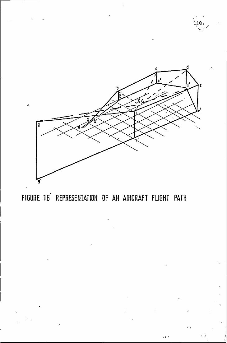
~
1;10. . ,-"_ r '
,
, FIGURE 16 REPRESENTATION OF AN AIRCRAFT FUGHT PATH
.. , , ,
·1

·HO
CD "0 ..... +
c; CD -c
lOO
- 90 '" ,. '" ..... '" '" <> = 80
•
• 110
lOO
<D
~ 90 +
<=> m "0
'" ~ 80 ..... '" '" '0
""
70
o ~
U >
'10
IS)
u
~ >
i i I 2
level-Exceedance Distribution of all Peaks
lA) LANDING AIRCRAFT i i I i i 5 10 20 50 . 80
Percentage !Total Distribution)
Clactonj Daventry Departures
I o
28R X Site '-----;7 ~ _l~-ndl;- -- ----
i I I I
Kilometres I i i i i
10 2;BR ~2Bl .I"..p
Mean Peak level
-Io-p
level - Excee dance 0 is trlbulion of all Peaks
(8) DEPARTING AIRCRAFT
111. .
I 90
~i~i~--rl--~I~--~i------~i------~i~--I
I 2 5 10 20 50 BD 90 Percentage (Total DistributIOn)
FIGURE17 DISTRIBUTION OF VARIOUS AIRCRAFT TO OVERALL -PEAK NOISE LEVEL DISTRIBUTIONS
:ll ,,'.F

•
Helght 1ft) (m)
4000 1200
1000
3000
800
2000 600
400
1000
200
o
Radar Tracked Data
la Median, light and Medium Jels(predomlnantly light)
X MedIan, Heavy Jets
5 10 Distance from Start of Run (km)
_x - ------~-X _ --
15
FIGURE 18 COMPARISON OF GENERALISED CLIMB PROFILES WITH RADAR
TRACKED DATA
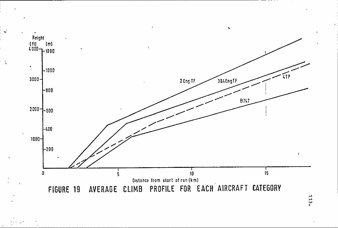
I
, -I '" •
Height (ft) (m) 4000 1200
1000
3000
800
2000 600
400
1000
200 ,
o 5 10 15 Distance from start of run (k m)
FIGURE 19 AVERAGE CLIMB PROFILE FOR EACH AIRCRAFT CATEGORY
- "
......
...... w •

,
(01
.. (510
Terrain 0 0 -Open ~
ill B '''''' Portly wOOded '0 '" HeaVily woode " = Grassy c
.Q 6 .. Source 0 :>
Obser~ c
" " :: <{
on 2 '" " u X III
0
ylt. Elevation angle: degrees
Effect of Terrain and Elevation Angle (150 -300Hzl (Reference 41 & L21
c: o
:;:. 10
" ~ B .. ... ~ ti 6 <t 0
o " ~~2 ~1l ... 0
10
~ / ~
V ~ ./ "'-....
lOO 1000 10000 Frequency; !1z
(bl Ground Attenualion over High Grass, Source and RecEiver 6ft above ground level (Reference 421
114.
10~------+-----~4---~--~------~------~
m '0
C .Q .. g c ! 20~------~~-------,~------~----~~~--------~ .. <( .. on Cl u. X III
30~----~------~------~----~----~ o 500 1000 1500 2000 Distance from source (metres)
(cl Downwind Ground to Ground Excess Attenuation (Reference 431
FIGURE 20 EXCESS ATTENUATioN DUE TO GROUND EFFECTS l '

13
12
'0'1 11 c::
..c ::> Cl "g
Cl> U c:: Cl
-; 10 "g
CD "g
:z: 0-. !! 9 o = c Cl . :;:: Cl ::> c:: Cl> -=i 8
Propagatlan Path Angle re Ground Plane (degrees]
FIGURE 21 AIRCRAFT NOISE PROPAGATION LAW ( E 0 U AT ION 4·4)
•
115.

,
130
120
, 110
--'
<>:100 -' :z: c.. -'"
'" QJ c..
90
2TF
4TP
60~--------~--------~--------~--------r-------~ o 5 10 15
Distance along route from start of run (km) 20 25
FIGURE 22 MEAN PEAK LEVEL (PL1) vs DISTANCE FROM START OF RUN
I •• ' \ •
(DEPARTURE ROUTES)
,

120
110
~ 100 ..
-'l '., "'-
-' :z: "'-
~ 90 QJ
"'-
80
70
, '
i
4TF Level Flight at 2000ft (S10m) - - - 747 (20001t)
-_~4If..!:.e'yel Flight at 3000ft(914m)
'~~~~U-~=-:///~~==::::7~4~7~(3~OO~O~I~t)== .:: / 4 TF(3°approach)
:~~~::::-~/~'2=&:3:T:F~(3~O~O~OI;t:):-______ __ -----<--:.:.--~4!}T!PE(3~O~OO~I~t)=:====747. 21. 3 TF
( 3°approach)
4T P (3° approach)
I i o 5 10 15 20
Distance to runway threshold (km) 25
FIGURE 23 MEAN PEAK LEVEL (PL1) vs DISTANCE FROM RUNWAY

Q:I "C
40
• ~30 <l c: <:> -u
'" ~ ~ <:>
<-> '" 2 0 c:
'" "C
en
10
(a) 2-engined Turbo-fan Aircraft
Sideline distance{kml 1'5 ~istance from start of run {kml
25
FIGURE 24 CORRECTION (b.L,) FOR SIDELINE DISTANCE FRor~ ROUTE (DEPARTURE ROUTES)

50
40
~ Sideline distance (km) .::; <l
.... .. l:: o
<-> .. c a; ::= 20 en
10 0-2
FIGURE 24 CONTINUED
( b) 3and4- engined Turbo-fan Aircraft
Distance from start of run (km)

-, '
: 50
40
~30 -.... <l '" o -U <l.I
~ 20 <..>
<l.I
'"
10
•
Sideline distance (km I
~3'0 4
FIGURE 24 CONTINUED
(c) 8747 AIRCRAFT
Distance from start of run (kml
.... '" o

... c:
50
40
10
Id) L..-engined Turbo-propeller Aircraft Sideline Distance (km)
Distance from start of run (km]
0·2 r--__ 25
FIGURE 24 CONCLUDED

.'
ID .." . ~ .....
50
40
~ 30 o
u Cl> ~ ~ o ...... Cl> c::
";;; 20 "0
en
10
,
Sideline DIstance (Km) o 1st ance from Runway Threshold (Km)
~-----____ 2 5
0-2
FIGURE 25 CORRECTION (~L1) FOR SIDELINE DISTANCES FROM ROUTE (APPROACH ROUTES)
,., I\) I\)
-
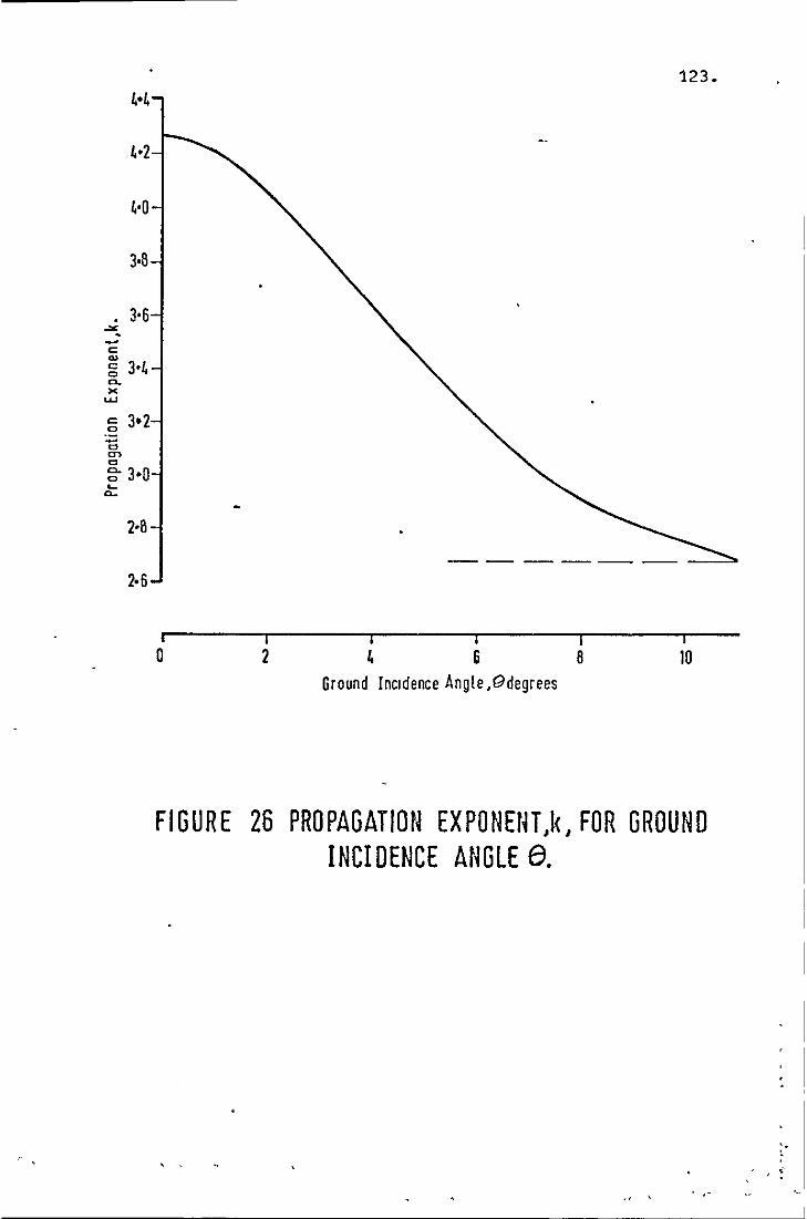
~.~
~'2
~·O
3·B
. JoG .>< . -c: .. gN CL ><
UJ
c:: 3-2 0
c; en '" g- 3'0 ~
"-
2·8
2·6
i I 0 2
123.
-------"'"
I ~
I 6
Ground Incidence Angle ,9degrees
I 6
I 10
FIGURE 26 PROPAGATION EXPONEfH,k , FOR GROUND INCIDENCE ANGLE e.
" ' , ,-
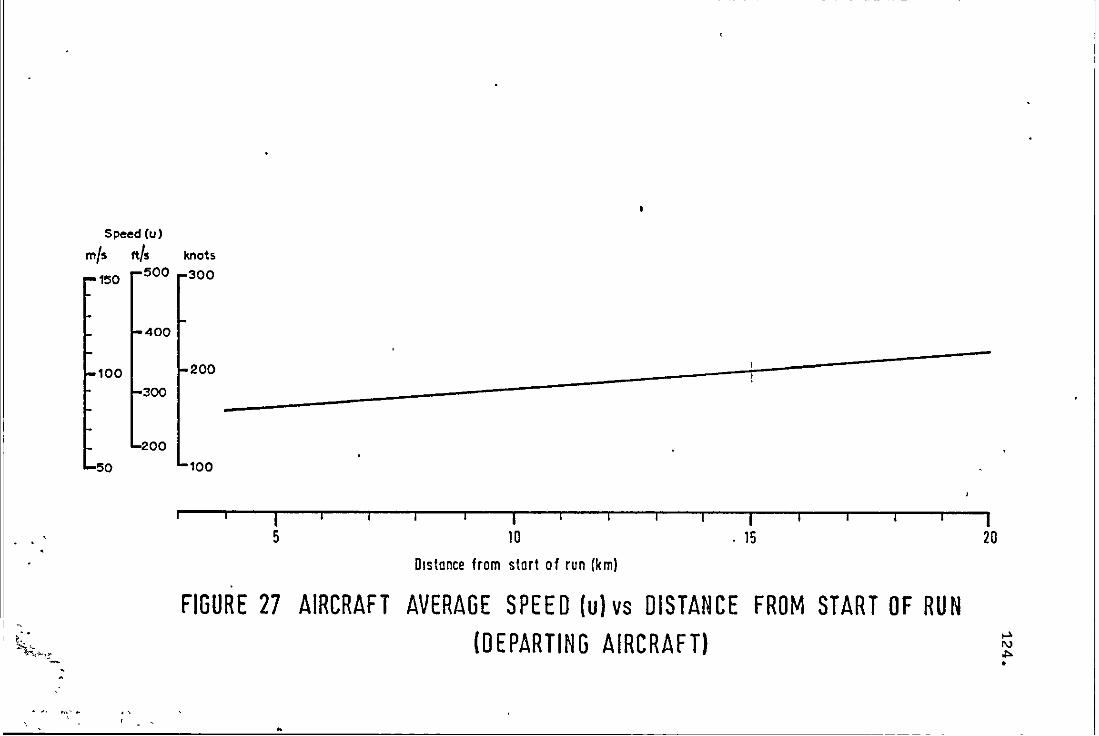
-----------------------------------------------------------------------------,
. .
Speed (u)
m/s ttls knots
1!50 500 300
400
100 200 __ ------------------+--------300
200
50 100
I 5
I 10
Distance from start of run (km)
I . 15
FIGURE 27 AIRCRAFT AVERAGE SPEED (u) vs DISTANCE FROM START OF RUN (DEPARTING AIRCRAFT)
I 20

J1.1=t :~
, , .,1, " ,le1illffi ,~~5 :,: 'ii:
I~ , ~ L"'~"" . ..c,-: 1--- -'5 I:-i'\ :: ') ,,'~'"'
I_·C[,,·'''' !'"
':c Il~F':,·:-· .' I~ : "I"'; I~ i ',' !-,dj":,·' 1 ": 'C;'LI "" 10'
, i:-. ,'= 1';-:' l:::
.':
HI. ;'-1 .. t:- I.:: t-· ..
, 'n- t; H"
1·0
,
p;. f:tt." I' 'L I li+: ' I
I I" fittHt.b.+ I I !.i ' I ,I
[ .. t· I;·" -_ , I " I I
" ,
- ,'" ~.. .. .. i._·.. 1-'1" ::. I', '. - ,. I:: i~ " V'·, ~i'··· i ,. :=I~_'" • ,,'1' .' "
.",," .~,~"!~/~ "~~'~'I-, b~'~.f~~:~:~
~li;I .. ':":! ++"';;' .~I·.IZ ,'7 I ".,r: ~ :'-.. i:'· .:~ " ' I,:.i=i· :::!-::: = 8: I .. ' '~"l;: '''r:'' V ,::;:' . '/ l=:;5 ~ ,~"r I:; I " . I ,:.~ L'. "" IF :.: =-,,: :.1,,, Y ~' -, :0: ~·.-~·I '" ;."' ,/. .:
C> ;~ Of': '" c:::I:,;', <'':: yr::::!:: I ;:'1:" ! ::C!;: I;!: " .....
, .. , .... t'= ,
0'01 -~ 3 4 5
, I
6 7
err (dB)
, "
," 11111 Ii" 11", 11'
8
, , ,
Ill, I I I i'" ,', I ~;li I:; i
9 10
FIGURE 28 RH.S. OF EQUATION 3.10 vs erp FOR A
, L~o -A IN 5 d BST E PS .
. , "
• ", :>

APPENDIX I 126.
AIRCRAFT NOISE MEASUREMENTS AT SITES NEAR HEATHROW AIRPORT
1. Measurement Procedures
The objective of this exercise was to obtain a large
sample of aircraft noise data corresponding to various
modes of aircraft operation in the near-airport vicinity.
To suit this purpose five sites were selected in the region
around Heathrow (London) Airport. These are shown in
Figure 1.1 in relation to the aircraft routes used on the
measurement day. Two sites are within a departure-route
region wher~ the noise would normally be attributable to
aircraft in a noise-abatement climb. One site is near the
three-degree approach path to Runway 28R and also allows
measurement of the approach flights to the more distant
28L runway. The two other sites are in a region where it
was hoped to measure "ground-to-ground" propagated noise
from aircraft in their maximum-power take-off ground run.
The condition of maximum-power overflight was not included
as it was receiving a separate and concentrated study
effort by Lanzer (Reference 32).
The period of measurement was from 07.00 to 19.00
hours (BST) on Tuesday, April 10, 1973. During this period
all 'arriving and departing aircraft used Runways 28R and
28L. Interchange of runway use (from landing to take-off
and vice-versa) occurred at 10.04, 12.30 and 16.14 hours
(BST). At all but one of the sites the noise data record
ing procedure was to commence tape recording when a flight

127.
could be positively identified as relevant to the pro-
gramme and to terminate recording when the sound had
diminished to an insignificant level. At one of the
"ground-to-ground propagation" sites the procedure was to
continuously record noise exposure with minimum interrupt-
ion.
Runway logs for the noise measurement period were
supplied by the Civil Aviation Authority. These originate
at Heathrow Air Traffic Control and comprise a listing of
each flight; with flight number, aircraft type, time of ,
event (GMT), runway used and route used. Meteorological
data for t~e period were obtained from the airport meteor
ological office and are reproduced here as Table 1.1.
The measuring and recording equipment at each site
comprised a sound level meter, acoustic calibrator, micro-
phone windscreen, tripod, Scotch 220 magnetic tapes, and
a Nagra IV-S magnetic tape recorder. The sound level
meters available for the exercise were Bruel and Kjaer
types 2203 (one), 2204 (two) and 2205 (two). These were
deployed according to the expected requirements of each
site noise condition. The B&K 2205 system is not a precis
ion sound level meter within the requirements of References
44 and 45 specifications. However, this limitation is due
only to the characteristics of its installed microphone
and can be disregarded when the system is used to meet
restricted measurement requirements. Calibration charts
for the available 2205 systems show the sensitivity to
frontal-incidence (0°) p~ane waves to be within 0.5dB
" ' .. 'I ,
.'

128.
(from nominal) over the frequency range 20Hz to 8kHz. The
systems were therefore considered adequate for measure-
ments at the "ground-to-ground-propagated" noise sites,
where the higher frequency sound content is of low magni
tude compared with the 20Hz to 8kHz range content. A
single direction of propagation at these sites was also
suited to the use of the 2205 systems. A disadvantage is
that of lower nominal sensitivity than other systems which
accommodate condenser-type microphones. Again, consider-,
ation of the expected level range of interest, down to
about 55PNdB (42dB(A) approx.) suggested the adequacy of the
type 2205 systems in this particular application. (These
have an inherent noise 'floor' of about 27dB(A).).
The B&K 2203 and 2204 sound level meters were used at
the flyover (or flyby) noise sites. While the author's
preference is to use B&K 4134 type, pressure-response,
microphones (in a grazing incidence orientation to the
flight path) for flyover noise measurements, this could
not be accommodated by the available range of equipment.
The SLM systems were therefore used with B&K 4133 (one)
md B&K 4145 (two) free field microphones installed. In
each application the microphone was oriented such that
the normal (00) incidence line was pointed towards the
closest point of flight approach (or the closest predict
able approximation to the CPA).
All recordings at all sites were made with a tape
transport speed of 7fips. A calibration signal was
recorded at the beginning of each tape by means of an
. '

129.
acoustical signal imposed at the microphone. Pistonphone
types B&K 4220 and 4230 were used. Windscreens (B&K type
U~ 0207 or UA 0237 according to microphone diameter) were
applied to the microphones, and these measurement units
were tripod-mounted at a height of 1.2 metres (about
4ft.) above ground level. Detailed logs of the data
acquisition history and signal-conditioning processes
imposed on the r,ecordings, were compiled throughout the
measurement programme.
2. Data Analysis
The tape-recorded data acquired at the flyover-noise
sites were analysed by means of a Bruel and Kjaer equip-
ment comprising (see Figure 1.2);
(a) Measuring Amplifier Type 2607
(b) Level Recorder Type 2305
(c) Statistical Distribution Analyser Type 4420
The recorded data on each tape were processed through
the analysis system twice. After calibration of the
output by means of the recorded reference signal, each
tape was played-back in a continuous (non-stop) mode to
provide a first-look time history trace of the D-weighted
sound level. While this was being produced on the Graphic
level recorder, the statistical distribution analyser was
processing the trace fluctuations to give a total cumu-
lative count of level exceedence data. Here, the distri
bution analyser was set to sample the trace level at
1/10 second intervals. The twelve counter indicators of
the analyser were set to provide a total cumulative count .. of the number of "instances" at which the D-weighted
, '
, , ,. , ~ ~ , .

,
,
130.
trace level exceeded SdB incremented levels of 60dB(D)
to 11SdB(D). This procedure was applied to all of the
recorded tapes for each flyover site. The total level-
exceedence counts for each site exposure were obtained by
summation of the respective indicator values for the site
tapes. These data correspond to the aircraft noise duration
statistics shown in Figure 5 of this report, where they
are presented as a percentile of the total measurement
period. The lower sound level percentiles are omitted where
they were obviously influenced by non-aircraft noises
and tape-gaps between event recordings.
The tapes were subsequently re-analysed through the
same equipment, but in this second analysis each flight
event was individually processed to provide the noise
duration statistics of its contribution to the exposure.
Guidance on analysis start and stop times was obtained
from the first-run time history traces. These individual
event analyses data were tabulated on computer-punching
data sheets as shown in Figure 1.3. The tabulation inclu-
ded, for each event, the tape number, event number,
event time (BST), aircraft type (coded), approximate dis
tance (coded), sound level meter range setting, total
count of 1/10 second instances at which trace exceeded
60dB(D), 6SdB(D), ••• to 100dB(D) in SdB steps, minimum
level (dB(D», of data validity, measurement operator
identity (coded), aircraft type (operator guess), coded
key to causes of possible error, peak sound level of
event (dB(D». With these datc\" punched on computer .cards,
, . ,
,
'"

,
131.
various forms of digital processing were then available.
Examples of these have been presented in"this report and
include the breakdown of peak levels by aircraft type,
numbers of peak levels above various sound levels, average
peak-energy levels and equivalent continuous energy levels.
The ground-to-ground propagated noi~e data acquired
at the two other sites were first processed by the same
analY,sis method to provide time-history ~races of the
D-weighted sound level, but not the statistical breakdown
of the temporal characteristics. Comparison of these
traces with the runway-logs provided an identification of
the aircraft events causing the noise excursions at the
nearer of the two sites. The traces obtained at the
further (from airport) site consisted of many sound level
excursions of similar magnitude to each other. These
could not be separated into aircraft and non-aircraft
events and further analysis of these particular records
was abandoned.
Peak D-weighted sound levels were then obtained from
the nearer-site data traces and compiled into sets for
each aircraft type operating from Runway 28L. These have
been presented in the report. Frequency analysis of some
selected records (for BAC 1-11 and DCS aircraft) was per
formed by repeating the time-history trace producti?n with
the input signal to the level recorder limited to octave
bandwidths. Synchronisation of these traces with the
D-weighted sound level traces allowed an octave-band
frequency spectrum to be compiled for each case of an
event noise peak (i.e. the peak D-weighted level). From
•• . .
" ,

132.
these spectra the corresponding values of Perceived Noise -
Level and D-weighted Sound Level were computed and co m-
pared. Since it is known that the peak PNL and D-weighted
sound level do not necessarily coincide (in time) for an
aircraft event, octave band spectra were developed for
instances 1 and 2 seconds prior to and after the peak
0- sound level occurrence, and PNL values computed from
these. These have been discussed in Section 4.4.
\ V

/
Table I.I Meteorological Data for Heathrow Airport on April 10, 1973
Temperature °c Wind Time Airfield Barometric GMT
Dry Bulb Wet Bulb Pressure m.bar Dlrectlono ,
0600 0.5 -0.4 1015.3 320
0700 1.7 0.4 1015.5 320
OBOO 3.5 1.4 1015.4 340
0900 5.5 2.6 1015.2 350
1000 7.3 3.2 1015.0 350
1100 B.4 3.2 1014.7 340
1200 9.1 3.8 1014.2 340
1300 10.0 4.4 1014.1 330
1400 10.5 4.7 1013.5 330
1500 10.7 4.9 1013.0 310
1600 10.6 5.2 1012.8 300
1700 10.6 5.2 1012.5 300
1800 10.4 4.9 1012.4 320 ,
vector
Speed (kts)
5
5
B
13
15
13
13
12 ,
10
11
11
11
11 ..... w w •

ffi Site 2
Site 1 E9 "",=::::~...::;:.Oe-spa;;;rt~ur.:.e :.:..::Ro.:.:ut=es_---::::=C===2=a=R===~,-L-and~a-th ___ ___ _
':----+------::~---;:;;;::-----c:=====:;:;== ________ _
28L
i o
Scale, km i i Z 3
I 4
I 5
FIGURE 1·1 MEASUREMENT SITE LOCATIONS
ffi Site 4
E9 Site 5

Nagra IV
Tape
Recorder
Measuring Amplifier
B&K 2607
Level
Recorder B&K 2305
Statistical Distribution
Analyser B&K 4420
Linear Record, Playback 7tips tape transport.
Direct Input D-weighting Filter
135.
SOdB logarithmic potentiometer Pot. range SOdS Lower Limiting Frequency 20Hz Rectifier Response, RMS Writing Speed 63mm/sec. Paper Speed 1mm/sec.
Cumulative Distribution 0.1 second sampling
FIGURE 1-2 ANALYSIS EQUIPMENT .,
, ,
• ,
•• I

LOUGHBOROUGH UNIVERSITY OF TECHNOLOGY, The Computer Centre Data Punching Form NAME [;cI. •• n.,J.s ..... t .... l. PROGRAM TITLE DATE Afi. 7~
Page I of 3
5 10 IS 20 2S 30 3S 40 4S 50 55 60 65 70 75 80
FIGURE 1·3 DATA INPUT FOR DIGITAL PROCESSING

137.
APPENDIX 11
DERIVATION OP NOIE EXPOSURE STATISTICAL DATA POR A SITE
NEAR LIVERPOOL AIRPORT AND A SITE NEAR MANCHESTER AIRPORT
The objective was to simulate the aircraft noise
exposures that would be experienced at the Heathrow site
#3 if the operations were restricted to those of smaller
regional airports. The noise exposure statistics result
ing from these simu1ations have been presented as Pigure 6
of this report.
As was described in the preceding Appendix, ~he
Heathrow noise data were compiled as computer input and
identified by site number, time and aircraft type, etc.
Por the present purpose, runway logs for Liverpool and
Manchester Airport operations were obtained and from
these the air-transport movements were extracted for the
12-hour period between 0600 and 1800hrs. GMT on
October 4, 1974. These movements were identified by air
craft type and time of departure. Noise data, including
peak level and duration counts, were then compiled for
these particular successions of events by extracting the
corresponding event data from the measured Heathrow Site 3
storage. In this procedure, the aircraft type identity
was rigorously maintained in the data extraction. The
event time (GMT) was also followed as closely as possible,
although this was not always feasible for some aircraft
types. Avoidance of using the same data in repetitive air
craft events was also intended, but could not be maintained
\ { ~, ., ~
138.
for the Ve8 type aircraft due to their more frequent usage
at the regional airports (than at Heathrow). Finally, the
data extraction process was limited to only those air
craft events that operated on the departure routes
closest to the Heathrow measurement site.
The Figure 6 presentation of peak level occurrence
and noise duration statistics was simply developed from
these simulated compilations. The peak level statistics
were expressed as a percentile of occurrence, above 5dB
incremented levels. The duration statistics were simi
larly expressed as a percentile of the 12-hour period
for which each level was exceeded.
~ - ...
t

139. APPENDIX III
ERRORS CAUSED BY NEGLECT OF TRUNCATION IN DISTRIBUTIONS OF
NOISE EXPOSURE
The Equivalent Continuous Energy Level, Leq , is of
current interest as a possible means of assessing a noise
exposure. Its fundamental definition is,
(1)
but it is equally expressable as
[
("."'" LilO ]
.Jo 10 .p(L).dL. (2)
where p(L) is the probability density of the statistical
distribution of the noise exposure (time-history) and L", ••
is the highest level' reached by the time-history.
It has become quite common in recent literature on
the subject to quote the approximation for
from the assumption of a Normal (Gaussian)
L that arises eq
probability
distribution with infinite upper limit. This is derivable
from (2) as
2 <JL 8.68
(3)
where LSO is the level exceeded for 50% of the time and
'Level and Sound Level are used here to mean some appropriately short-time averaged and weighted measure of noise exposure level •.

140.
2 ~ is the variance of the sound level fluctuations.
The errors associated with this approximation can be
large, even when the exposure statistics appear to be
Normally distributed over most of the level range. Of
greatest sig~ificance is the effect of an abrupt truncation
of the distribution at some level,
as is shown in Figure 111.1. Because of this truncation
there will also be a departure from Normalcy at the lower
levels of exposures. The effect of this on Leq is usually
insignificant due to the much lower order of energy con
tribution.
Now, for the truncated' distribution, Leq can be
approximated as,
where
L eq J LSO+!lar:.
= 1010g10
LSO- co
L/10 10 .p(L) .dL
1 p(L) = --=--~j2rr
2
(-(L - LSO) )
.exp 2 2<7[.
,., Substituting (5) into (4) with L =(L- Lso)/OL'
which reduces to
(4)
(5)

2 C1i
8.68
141.
_Z2/2 J e .dz.
........................ 61,/10
where b = 2.31~/10 (i.e. b = loge10 )
"" and z = L - b , This gives equation (3) when k = 00
For finite k' (that is, a truncated distribution),
2 <T"L
= LSO + 8.68 - 3 + k' - b
+ erf (
.. .. .. - .. .. .. .. .. .. .. ..
where erf is the well-known error function.
Comparing equations (3) and (7) it is immediately
obvious that the difference will be less than 3dB when
the erf argument m greater than zero. This means that
( 6)
(7)
for equation (3) to give Leq within 3dB, the distribution
of noise exposure must be Normal up to a level of at least,
= , dB.
The error caused by using equation (3) for other truncated
distributions, which are Normal between the truncation
limit and some very low level, can be evaluated from
equation (7). Table 111.1 gives approximate values of
these' errors for various combinations of or. and A, where
~(equal to ~) is the interval in dB above LSO at which
\ ,

-------- -----------------------------
142.
truncation occurs. This table should be used as a guide
to the potential error, not as a compilation of correction
factors. Where unacceptable error is indicated by the
table, L should be evaluated by means of eq equations
(1) or (2). The average peak-energy level (L) of the
peak distribution can be similarly expressed as
_ A 0-: 2 [ L = LSO + ~ - 3 + 1010910 1 + erf (
. . . . . . . . . . . . . . (8)
, where the truncation limit is LSO + kap' and b = 2.31iP/10.
Table 111.1 can be used to assess the potential
error caused by using,
2 ~ 8.68
on the peak level distribution.
The effect of an 80PNdB cut-off on the range of
significance is not so readily estimated. This effect
is introduced in the NNI formula, where L is evaluated
for peaks in excess of 80PNdB. If thE cut-off is
expressed in similar form to the truncation level, that
is, A
80PNdB = LSO + € op
then an equation similar to (6) can be developed. In
the peak distribution notation, equation (6) becomes 2 r{_b _z21P' ] - A ~ [1 L = LSO+ 8.68 + 1010g10 J 21T, e., .dz (9)
E-b

where b = 2.310-/10 P
In this case the equivalent of equation (7) is,
2 CT"p 8.68 - 3 +
r. It-b €-b)ll 10log
10Lerf (~)- erf(v 2j
143.
............... (10)
, So, if k is very large and positive (indicating an upper
truncation limit well in excess of 150 + op2/ 4.34), and£
is very large and negative (indicating that the 80PNdB level A 2 '
is well below LSO + op /4.34) then the approximation
2 .2..
+ 8.68
is again given.
The correction to this approximation, allowing for both
cut-off and truncation, is best evaluated by means of
equation (10). Tables of error function values are given
in many text-books on statistics and standard functions.
One such source is Reference 46.

TABLE III.I Difference (dB) in L for Innni te and Abruptly Truncated "Normal" eq
Distributions of Noise Exposure·
A standard Deviation ~ (dB) , (dB) 4 5 6 7 8 9 10 12
.
35 1 3
30 1 4
25 Less than ldB 1 3 6
20 1 3 4 9
15 1 2 3 5 7
10 1 2 3 6 8 10
8 1 2 3 4 7 9 Greater
6 2 3 5 7 9 than 10dB
4 3 4 6 S 10 I ·see Figure III.l
l:::. .. interval, above L50 where abrupt truncation occurs.
~ is the standard deviation calculated by (L10 - L50 )/1.2S.
14
7
9
10
, \
•

.-L "" '" ~ Truncation Level
t-r ~~ lOdB
-0 cu
"C cu cu u ><
6=k'o- ~
QJ - --
~
145 •
~ ~
cu Lso >cu -'
--------------~ ! ",,-x= Measured data
: " 05 1 2 5 10 20 50 90 95
0,. Time for which level is exceeded (Gaussian base)
FIGURE m·, ILLUSTRATION OF TRUNCATION LIMIT
, ,
, / " " ,

APPENDIX IV 146.
AN EXAMPLE SITE NOISE 'EXPOSURE PREDICTION
The case to be considered is that of a site which is
1.3km to the side of an airport departure route ground
trace. The distance along this route trace, frq~ the
start of run point on the runway to the nearest approach
point relative to the site, is 15km. The aircraft fleet
mix using the route, averaged for a 12-hour daytime period
(0600 to 1800hrs. GMT) over a three-month summer season is;
B747 7%
4 engined TF 15%
3 engined TF 24%
2 engined TF 32%
4 engined TP 22%
and the average number of flights on the route is 48 per
12-hour day.
From Figures 22 and 24, the following values of PL1 and ~Ll are obtained and PL2 = PL1 AL1calculated:
A.C. PL1 A\ PL2
-B747 98.5 9 89.5 .. t
4TF 100 6.5 93.5
3TF 95 6.5 88.5
2TF 93 5 88
4TP 89.5 6.5 83
PNdB PNdB PNdB.

147.
The PL2
values a~e inse~ted in Table IX (page a9) and the
pe~centages of peaks in each noise level"band a~e calculated
acco~ding to the definitions in Section 5.1. The column
totals a~e calculated and the probabilities of exceedence
obtained by right-to-left cumulative summation of these.
Figu~e IV.l shows a g~aphical plot of the level-exceedence
pe~centages using No~mal Distribution graph paper. An
interpolative dist~ibution line has been superimposed.
An estimate of the Noise and Numbe~ Index (NNI) can
be obtained by means of this g~aph. Fi~st, the number of
flights exceeding aOPNdB is given as a9% of the ave~age
daily total. That is,
Nao = 0.89 x 4a = 42.7, and
= 24.4
Next, the average peak-ene~gy level, Lao ' of these flights
is ~equired. This can be obtained by three diffe~ent
methods discussed in this report.
(a) Equation 2.9 can be used as a graphical integration
method. This is worked out in Table IV.I, with the result
Lao = 90.5PNdB.
(b) Equation 2.7 can be used provided the effects of distri
bution truncation at aOPNdB and 105PNdB a~e small. F~om
A the graph it is observed that LSO = 87PNdB and that A A L10 - LSO = 7.2PNdB.
Taking
= = S.6PNdB,
"

Equation (2.7) gives
2 It. ~ = L = LSO + 8.68 90.6PNdB.
The effect of truncatiom is included in the following
method:
148.
(c) Equation (10) of Appendix Ill) can be used. The upper
truncation limit is expressed by
A
k' = 105 - LSO = 3.22
op
The lower truncation limit is expressed by
1\
80 - LSO E. == == ap
-1.24
The value of b is also required.
b == 2.31 op/l0 = 1.29
Now,
Lao = L (from the previous method) - 3PNdB
[ k'-b £-b J + 1010g10 erf(---) - erf(---) n J2
, where (k-b) = 1.36, erf == 0.946
~ .. (~) = -2.53, erf == -1.0 n
Therefore,
Lao = 90.6 - 3 + 1010910 [:.946J
== 90.SPNdB.
, . ;.- . '
149.
The value of NNI is therefore,
NNI = 90.5"+ 24.4 - 80 = 34.9
An estimate of Leq can be obtained by means of gquations
3,14 or 3.15. The latter gives
2 = L + 1010g10n + 1010g101P - JP /65.8 - 29.5
+ 1010910(h/10U)
Substituting L = 90.6PNdB, n = 48/12 = 4 per hr.,
and 0- = 5.6PNdB, P
Leq = 74.1PNdB + 1010g(h/10U)
From Figure 19 and the percentage usage of the route, the
average height of the aircraft at the closest approach point
is 970 ~etres (3190ft.). With the sideline distance of
1300 metres, the average slant range is 1620 metres.
i.e. h = 1620 metres
From Figure 27, the average aircraft speed at the closest
approach point is 103 metres/second,
i.e. U = 103 metres/sec.
Therefore, L = 76.1PNdB. . eq
other noise duration characteristics can be obtained by
development of the level-exceedence time distribution, as
described in Section 5.2. For this, a facsimile of Table XIII
is used (Table IV.II of this Appendix).
Following the steps given in Section 5.2, the values
to be-inserted in the table are,
..

lS0. r = 1620 metres
k = 2.67
U = 103 metres/second
0(... = 99.4
Figure 28 is now used to obtain values for the right
hand-side (RHS) of equation 3.10. Tnese are shown in the
Table and correspond to op = S.6PNdB. peA) is calculated
and inserted in the table.
The final step in developing the level-exceedence
distribution of noise durations is to plot these values
(in percentage units) on Figure IV.l. ...
The LSO level is
used as a reference.
Indices such as L1 , L10 , etc., can be directly
obtained by interpolation.
Leq can be obtained by means of Equation 2.9, with
change of notation from peak levels to level exceedences.
A working chart of this graphical integration procedure
is given as Table IV.III. The value obtained by this
method is,
L . = 76.7PNdB eq
which compares well with the previous estimate. ~ ..

~-------------------------------------------
Table IV.I Evaluation of LSO by Means of Equation 2.9
(1) (2) (3) ( 4) ( 5) (6 )
" Lit 10 A 1\
Li 10 ~ P(Li -2.5dB) P(Li
+2.5dB) (3)-(4) (5)x(2)/100%
100 10xl09 3.0% 0.3% 2.7% 27xl0 7
95 3.16xl0 9 16.5% 3.0% 13.5% 42.6xl0 7
90 lxl09 46.0% 16.5% 29.5% 29.5xl07
SS .32xl09 79.0% 46.0% 33.0% 10. 5xl0 7
SO· .13xl09 • S9.0%" 79.0% 10.0% 1.3xl07
2: column (6) = 110. 9xl0 7
LSO = 10l0910(110.9Xl07
) = 90.5PNdB
"The SOPNdB limit is applied to this stratum.

Table IV.II Method fo~ the Evaluation of peA)
Equation 3.10, fo~ va~iable k, is A " A _A )2
2.34 ~ 3 (LSO -)..) [ LSO -). ] ~ -(LSO .xl0 XP(A).. 2 1 + e~f ( ) + ....:..I?- expo ( 2 ) n [2'0- {2rr 2 ap .
P
k = (f~om Figu~e 26)=2.67 h .. 1620m n = 4 pe~ hour
U .. (from Figu~e 27 ).103m/sec. u/h ... 064 3 ka 99.4 a .. ol..= 2.34xl0 .-. = n
" -), LSO ' dB
-15 -10 -5 0 +5 +10 +15
RHS (F~om Figu~e 28) 15 10 5.6 2.2 .54 .09 ,
pO,) RHS .15 .1 .056 .022 .0054 .0009 .. --~

Table IV. III Svaluation of Leq by Means of Sguat10n 2.9
(1) (2) (3) (4)
Li 10 L1/ 10 P(Li -2.5dB) P(L
i+2.5dB)
97 5x10⁹ .25% .03%
92 1.58x10⁹ 1.1 % .25%
87 .5x109 3.6 % 1.1 % 82 .16x109 8.0 % 3.6 %
77 .05x109 12.5 % 8.0 %
72 .016x109 17.5 % 12.5 %
Leq = 1010910 (4.69x10⁷ ) = 76.7PNdB
(5)
(3)-(4)
.22%
.85%
2.5 % 4.4 % 4.5 % 5.0 %
.Gcolumn (6) =
(6)
(5)x(2)/100%
1.10x10 7
1.34x10⁷
1.25x10 7
.70x107
• 22x10 7
.08x10 7
4.69x10⁷
.... U1 W •
•

------------------ - - --
, FIGURE N·l

REFERENCED LITERATURE
(a) Loughborough University Reports
J.B. Ollerhead "Estimating Community Annoyance due to
Aircraft Noise" LUT TT 7203, 1972.
155.
J. B. Ollerhead "Noise and Airport Planning" Proceedings of
a Conference on Airports of the Future, Tel Aviv, 1972.
J.B. Ollerhead "Methods for Quantifying the Effects of ,
Noise on People" Proc.Brit.Acoust.Soc., 2, 2, 1973.
J.B. Ollerhead "Aircraft Noise: How can the Nuisance be
Controlled?" Applied Ergonomics, 4, 3, 1973.
J.B. Ollerhead "Estimating the Nuisance Caused by Transport-
ation Noise" Proc. of Symposium on Transport and the
Environment, Loughborough, 1973.
J.B. Ollerhead "Thoughts on a General Model for Predicting
Community Response to Noise" Proc.Brit.Acoust.Soc. 2, 3,
1973.
J.B. Ollerhead "The Case for a Unified Approach to the
Assessment of Long Term Unsteady Noise Exposure" Proc.Brit.
Acoust.Soc. 2, 3 (1973).
E.J. Richards and J.B. Ollerhead "Noise Burden Factor: New
Way of Rating Airport Noise" Sound & Vibration 7, 12, 1973.
J.B. Ollerhead and R.M. Edwards "Measurement of Airport Noise
Impact on Residential Communities Near Airports" 8th ICA,
1974.
R • M. Edwards, "A Survey of Aircraft Noise Annoyance in
An Area of Invariant Noise" LUT TT 7405, 1974. To be
published in J.Sound Vib., May 1975.

J.B Ollerhead and R.M. Edwards "A Further Survey of
Aircraft Noise Impact in Residential Communities Near
London (Heathrow) Airport" LUT TT report in preparation.
J.B. Ollerhead, D. Brown, R.M. Edwards "A Comparitive
Study of Aircraft Noise Nuisance at Three Airports"
LUT TT Report in preparation.
M. Lanzer "Analysis of Aircraft Take-off Noise"
LUT TT ., 1975.
N. Deva-Aditya, R.D. Hooper and J.B. Ollerhead "Noise
Burdens at British Regional Airports" LUT TT ., 1974.
N. Deva-Aditya and J.B. Ollerhead "Criteria for Assess
ing the Acceptability of Airport Noise Nuisance
Volume 1 The Role of Social Justice
Volume 2 Applications of Social Justice Principles"
LUT TT· 1975.
N. Deva-Aditya and J.B. Ollerhead '''Noise Burdens at U.S.
Airports" LUT TT ., 1975.
(b) Text References
156.
1. Kryter, K.D. "Scaling Human Reactions to the Sound
fron. Aircraft" Jnl.Acoustical Soc. of America, Vol. 31,
No. 11 (Nov. 1959).
2. Kryter, K.D. and Pearsons, K.S. "Some Effects of the
Spectral Content and Duration on Perceived Noise Level"
Jnl.Acoust.Soc.Am., Vol. 35, pp. 866-883, (1963).
• Reports presently under review - not yet assigned numbers •
•• ,>\'

--- ----------------------------------------------------------------------------
157.
3. Ollerhead, J.B. "An ,Evaluation of Methods for Scaling
Aircraft Noise Perception" NASA CR-1883, (1971).
4. Adcock, B.O. and Ollerhead, J.B., "Effective
Perceived Noise Level Evaluated for STOL and Other
Aircraft Sounds" U.S. Federal Aviation Admini3t:ration
Report FAA-NO-70-5, (1970).
5. Committee on the Problem of Noise "Noise - Final
Report" HMSO, Repr. 1968.
6. McKennell, A.C. "Aircraft Noise Annoyance Around
London (Heathrow) Airport" Central Office of
Information S.S. 337, (1963).
7. Central London Noise Survey, 1961-62; see Ref. 5 and
McKennell, A.C. and Hunt, E.A. "Noise Annoyance in
Central London", Central Office of Information SS 332
(1968) •
8. Griffiths, 1.0. and Langdon, F.J. "Subjective Res-
ponse to Road Traffic Noise" Building Research Station,
Current Paper 37/68, (1968).
9. Langdon, F.J. and Scholes, W.E. "The Traffic Noise
Index: ,A Method of Controlling Noise Nuisance"
Building Research Station Current Paper 38/68, (1968).
10. Scholes, W.E. "Traffic Noise Criteria" Building
Research Station Current Paper 38/69, (1969).
11. Dept. of Environment, "Building and Buildings, the
Noise Insulation Regulations 1973" Statutory Instrument
No. 1363, HMSO, (1973).
','
--- ---- -- -- - - -------------~

158.
12. International Standards Organization "Assessment of
Noise with Respect to Community Response" ISO/R 1996,
(1971).
13. International Standards Organization ."Procedure for
Describing Aircraft Noise Around an Airport" ISO/R
507, (1970).
14. Robinson, D.W. "The Concept of Noise Pollution Level"
NPL Aero Report Ac. 38, (1969).
15. Fuller, H.C. and Robinson, D.W. "Subjective Reactions
to Steady and Varying Noise Environments" NPL
Acoustics Report Ac 62 (1973).
16. Robinson, 0.1'/. "An Essay in the Comparison of Environ
mental Noise Measures and Prospects for a Unified
Index" NPL Acoustics Report Ac. 59, (1972).
17. Report by a Working Party for the Research Sub
committee of the Noise Advisory Council "Noise
Units" HMSO (1975).
18. MIL Research Ltd., "Second Survey of Aircraft Noise
Annoyance Around London (Heathrow) Airport" HMSO,
(1971) •
19. Report by the Research Sub-committee of the Noise
Advisory Council "Aircraft Noise: Should the Noise
and Number Index be Revised?" HMSO, 1972.
20. Civil Aviation Authority "The General Aviation
Flight Guide" HMSO.
159.
21. Anon. "Aerad t'light Guide - S.I.D.'s" Airport Charts
published by International Aeradio Ltd., London.
22. Anon. "Aerad Flight Guide - Area Charts" Airport
region charts published by Int. Aeradio Ltd.
23. Anon. "Noise Abatement" Airport Bulletin published
by Int. Aeradio Ltd.
24. Bishop, D.E. and Horonjeff, R.D. "Procedures for
Developing Noise Exposure Forecast Areas for Aircraft
Flight Operations" U.S. Dept. of Transportation,
FAA DS-67-10, (August 1967).
25. Bishop, D.E. and Simpson, M.A. "Noise Exposure Fore-
cast Contours for 1967, 1970 and 1975 Operations at
Selected Airports" U.S. Federal Aviation Admini-
stration Report FAA-NO-70-8, (1970).
26. Galloway, W.J. and Bishop, D.E. "Noise Exposure Fore-
casts: Evolution, Evaluation, Extensions and Land
Use Interpretations" U.S. Federal Aviation Administrat-
ion Report FAA NO-70-9 (August 1970).
27. Tracor Inc., "Community Reaction to Airport Noise,
Vol. I" NASA CR-1761, (1971).
28. U.S. Department of Housing and Urban Development (HUD),
Circular 1390.2.
29. U.S. Department of Housing and Urban Development
(HUD), "Noise Assessment Guidelines".
30. Wyle Laboratories, "Community Noise" U.S. Environment-
al Protection Agency Report NTID 300.3, (1971).
,
I
-I

160.
31. Schultz, T.J. "Noise Assessment Gui?e Line, Technical
Background for Noise Assessment in HUO's Operating
Programs" U.S. HUO TE/MA 172 (1971). This report
has not been reviewed. The criteria have been repro
duced in other reports.
32. Lanzer, M. and Ollerhead, J.B. "Analysis of Aircraft
Take-off Noise" Loughborough University of
Technology Report.
33. Copeland, W.L. et al "Noise Measurement Evaluations
of Various Take-off/Climb-out Profiles of a Four
engine Turbojet Transport Airplane" NASA TN 0-3715,
(2966).
34. Bishop, O.E. "Frequency Spectrum and Time Duration
Descriptions of Aircraft Flyover Noise Signals" FAA
Technical Report OS-67-6, (1967).
35. Dredge, M., Brown, O. and Ollerhead, J.B. "Computation
of Airport Noise Exposure Contours" Loughborough
University of Technology Report.
36. Horonjeff, R. and Soroka, W.W. "Transportation System
Noise Generation, Propagation and Alleviation, Phase 1,
Part 1" U.S. Oept. of Transportation Technical
Report No. 00T-OST-ONA-71-2 (1970).
37. Civil Aviation Authority, "CAA Monthly Statistics"
CAA, London, (1973).
38. de Wit, G.A.M. "On the Noise i!l the Vicinity of the
Brussels National Airport" Proceedings of the 5th,and

6th International Congresses of AICB, London 1968
and Groningen 1970.
161.
39. Loughborough Consultants Ltd. "Aircraft Noise Datum
Levels Used for Airport Assessments".
40. International Civil Aviation Organization "Report of
the Special Meeting on Aircraft Noise in the Vicinity
of Aerodromes" ICAO Doc. 8857, NOISE, (1969).
41. Hubbard, H.H. and Maglieri, U.K. "An Investigation
of Sound Phenomena Relating to the Aural Detection
of Airplanes" NACA TN 4337 (1958).
42. Wyle Laboratories Research Staff "Sonic and Vibration
Environments for Ground Facilities - a Design
Manual" Wyle Labs. Report WR 68-2 (for NASA), (1968).
43. Franken, P.A. and Bishop, D.E. "The Propagation of
Sound from Airport Ground Operations" NASA CR 767
(1967) •
44. International Electrotechnical Commission "Precisbn
Sound Level Meters" IEC Recommendation, Publication
179 (1965).
45. British Standards Institute "Specification for a
Precision Sound Level Meter" B.S. 4197 (1967).
46. Jahnke, E. and Emde, F. "Tables of Functions"
Dover Publications Inc.
.'


![Environmental Mercury Exposure and the Risk of Autism edita...autism is reiterated in a study of baby teeth [4]. In this study, mercury in baby’s teeth represented cumulative exposure](https://img.pdfslide.us/doc/110x75/5eddf203ad6a402d6669304b/environmental-mercury-exposure-and-the-risk-of-autism-edita-autism-is-reiterated.jpg)