IZA DP No. 1295

The Enrollment Effect of SecondarySchool Fees in Post-War Germany

Regina T. Riphahn

DI

SC

US

SI

ON

PA

PE

R S

ER

IE

S

Forschungsinstitutzur Zukunft der ArbeitInstitute for the Studyof Labor

September 2004

The Enrollment Effect of Secondary School Fees in Post-War Germany

Regina T. Riphahn University of Basel,

DIW Berlin and IZA Bonn

Discussion Paper No. 1295 September 2004

IZA

P.O. Box 7240 53072 Bonn

Germany

Phone: +49-228-3894-0 Fax: +49-228-3894-180

Email: iza@iza.org

Any opinions expressed here are those of the author(s) and not those of the institute. Research disseminated by IZA may include views on policy, but the institute itself takes no institutional policy positions. The Institute for the Study of Labor (IZA) in Bonn is a local and virtual international research center and a place of communication between science, politics and business. IZA is an independent nonprofit company supported by Deutsche Post World Net. The center is associated with the University of Bonn and offers a stimulating research environment through its research networks, research support, and visitors and doctoral programs. IZA engages in (i) original and internationally competitive research in all fields of labor economics, (ii) development of policy concepts, and (iii) dissemination of research results and concepts to the interested public. IZA Discussion Papers often represent preliminary work and are circulated to encourage discussion. Citation of such a paper should account for its provisional character. A revised version may be available directly from the author.

IZA Discussion Paper No. 1295 September 2004

ABSTRACT

The Enrollment Effect of Secondary School Fees in Post-War Germany∗

This study utilizes the heterogeneity of the fee abolition for West German secondary schools to identify its effect on enrollment and to obtain an estimate of the price elasticity of demand for education. The analysis is based on administrative school enrollment statistics as well as on representative individual-level data from three annual surveys of the German Mikrozensus. Estimates suggest that enrollment in Advanced Schools increased by about six percent due to the fee abolition, where the results are sensitive to the specification choice. The positive enrollment effect of fee abolition for women exceeds that for men. A fifty percent reduction in fees is associated with an overall change in enrollment rates by 3 percent, where the elasticity of the demand for females' education again exceeds that for males'. JEL Classification: I20, H52, H71, C21 Keywords: school fees, tuition, enrollment, demand for education, natural experiment Regina T. Riphahn WWZ University of Basel Post Box 517 4003 Basel Switzerland Email: regina.riphahn@unibas.ch

∗ I thank Katja C. Fischer, Elsa Fontainha, Jörn-Steffen Pischke, Patrick Puhani, Kjell Salvanes, and seminar participants at MPI-Rostock, the Universities of Zurich, Bern, Mannheim, and Lausanne, at IFS (London), as well as the ESSLE 2003, and CEPR-Uppsala meeting 2003 for helpful comments and Joachim Benatzky for excellent research assistance.

1 The literature addresses this endogeneity using a variety of natural experiments (e.g.involving the GI Bill, tuition, or subsidy changes). For a survey see Dynarski (2002). Keycontributions are Kane (1994, 1995), Ichimura and Taber (2002), or Heckman et al. (1998).

2 Examples are Vermeersch (2002) on school meals in Kenya, Miguel and Kremer(2004) on deworming pupils in Kenya, Schultz (2000) on cash transfers to Mexican parents, orKim et al. (1999) on subsidies for girls' education in Pakistan.

1

1. Introduction

In industrialized countries secondary education is typically provided free of charge. This

is commonly justified by positive externalities, equity, and distributive justice arguments.

Historically, school fees were the rule at public schools and they are still commonplace for

private schools. Even though economic theory suggests that the demand for schooling responds

to its price and the price of schooling has changed over the last decades, we know little about the

effects of these price changes. Studies on the development of educational attainment over time

often do not account for price changes, and generally, the price elasticity of secondary schooling

has found little research attention compared e.g. to the price elasticity of college enrollment.

I take advantage of a natural experiment in post-war Germany to identify and estimate

the effect of (the abolition of) school fees on school enrollment and the price elasticity of demand

for secondary education. This contributes to several ongoing debates. First, the results are

informative for the discussion of school vouchers in the United States (e.g. Ladd 2002, Neal

2002, Epple and Romano 1998, Epple et al. 2004) where the cost of secondary education and its

behavioral effect is an important aspect. Second, the debates on the effect of tuition subsidies in

the United States and on the introduction of university fees in Europe generally lack reliable

measures of the price elasticity of education demand: In Europe, data on prior experiences with

academic fees are often unavailable. In the U.S., the measurement of the effect of public aid on

college enrollment is hampered by the potential endogeneity of aid receipt.1 The evidence

presented here is relevant to both of these discussions. Third, this study is related to a growing

literature that investigates instruments to increase school attendance in developing2 as well as in

3 See Meghir and Palme (2003) for the Swedish experience in the 1950s and 1960s,Aakvik et al. (2003) on Norway, and Dearden et al. (2003) for a current program in the UnitedKingdom.

4 Goldin (1998) points out that in the United States, where secondary education wasprovided generally free of charge, high school enrollment rates rose from 18 to 73 percent andgraduation rates from 9 to 51 percent between 1910 and 1940. Goldin and Katz (2003)investigate the role of compulsory schooling laws in this development. As Advanced Schoolparticipation until today exceeds the minimum requirements of compulsory schooling laws inGermany, these regulations are not relevant to this analysis.

2

industrialized countries.3 Finally, following up on Goldin (1998) and Goldin and Katz (1997) I

provide an analysis of secondary schools in Germany, which did not experience anything similar

to the North American increase in graduation rates in the first half of the century.4 I investigate

whether the existence of school fees contributes to explain the international difference in

educational enrollment.

Up until the end of World War II, fees had to be paid for advanced secondary education

in Germany, typically amounting to about ten percent of an average worker's gross earnings per

pupil. After the war, when educational authority was returned to the federal states, fees for

advanced secondary education were abolished state by state between 1947 and 1962. The

variation in the timing of fee abolition across regions is used here to identify the effect of fees

on Advanced School enrollment, and to compare the price responsiveness of demand for the

education of male and female youth. The analysis first investigates the responsiveness of

education demand to the existence of a school fee, and then it evaluates the sensitivity of

enrollment to changes in the price of education.

I find surprisingly small but significant effects of school fee abolition on enrollment. The

responsiveness of the demand for female education exceeds that of the demand for male

education. Overall, fee abolition seems to be associated with an increase in enrollment rates by

about 6 percent. A drop in the fee-to-income ratio by 50 percent or five percentage points

increases the aggregate enrollment rate by about 3 percent again with larger effects for females

5 Depending on region and period more or less demanding entrance exams were requiredto enter Middle or Advanced School (cf. Kuhlmann 1970).

3

than for males.

2. Institutional Background, Theoretical Model, and Hypotheses

2.1 School Fees in a Historical Perspective

Traditionally and until today, the German schooling system has been structured not only

by years of schooling, but also by parallel tracks with different performance requirements. Since

the 19th century the standard education has been provided by Basic Schools (Volksschule /

Hauptschule) which used to last 8 years and prepared pupils for apprenticeships or vocational

schools. It was possible to advance from Basic School after 4 years to either Middle School

(Realschule / Mittelschule) or Advanced School (Gymnasium / Oberschule),5 where education

continued for an additional 6 or 9 years, respectively (cf. Figure 1). The system hardly changed

over time, and the Advanced School degree remained the key requirement for university studies.

Through the 19th century there was a fee to be paid for any type of school financing

teacher salaries. Starting with Prussia (1888) and ending with Saxony (1919) fees for Basic

Schools were abolished state by state by 1920 (Kahlert 1974). The regulations on school fees for

Middle and Advanced Schools varied across regions. The fees per pupil at times exceeded 10

percent of an average labor income. Figure 2 depicts the share of school fees in average income

for the case of Prussia. It reflects nominally rising earnings during the inflation when fees

remained unadjusted. Around the time of WWII the German educational system was centralized

and underwent major distortions connected to the manpower needs of the military (for an

evaluation see Ichino and Winter-Ebmer 2004): Advanced School education was reduced by one

year in 1938, and starting 1941 it was at times shortened by an additional 6 months. Also, for the

the birth cohorts 1922-1928 final examination requirements were reduced and frequently dropped

6 We describe only the developments in former West Germany. School fees wereabolished for all of East Germany in 1957 (Geissler 2000).

4

completely to facilitate military service.

After the war, the authority for the administration of the school system was returned to

the German federal states. They increased the duration of Advanced School education back to

9 years and - instigated in part by the political ideas of the allied occupation forces (Furck 1998) -

re-regulated the fee system: Starting with the city-state of Bremen (1947) and ending with

Rhineland-Palatinate (1962) over time all states abolished tuition fees for public secondary

schools (Benatzky 2001, Berger and Ehmann 2000). While until 1945 the annual fee level was

set uniformly at 240 Reichsmark, there was considerable regional variation in the speed and

extent of fee abolition afterwards, which we use to identify its effects. Figure 3 describes the fee

abolition pattern across the 11 federal states.6 Frequently, tuition was abolished stepwise, e.g.

annually by one seventh over the course of 7 years as in the case of Hamburg, or in steps from

100, to 50, and 25 percent of the original amount as in the case of Bavaria. Figure 4 describes the

development of school fees per pupil by state and over time as a share of average earnings for

selected states. It shows the heterogeneity of the abolition process between 1947 and 1962.

In our analysis, we distinguish three cohort groups among the youths growing up in a

given state, based on the fee system they faced when entering Advanced School: The first and

oldest group would have had to pay school fees upon entering Advanced School (pre group). For

a second group it depended on the speed at which they completed primary education whether

they would have entered Advanced School prior to the abolition of the school fees (transitional

group). For these individuals we cannot tell for sure under which regime they attended school.

Finally, the third group consists of those birth cohorts who certainly would not have had to pay

school fees, because they entered Advanced School after the fee abolition (post group). Since fees

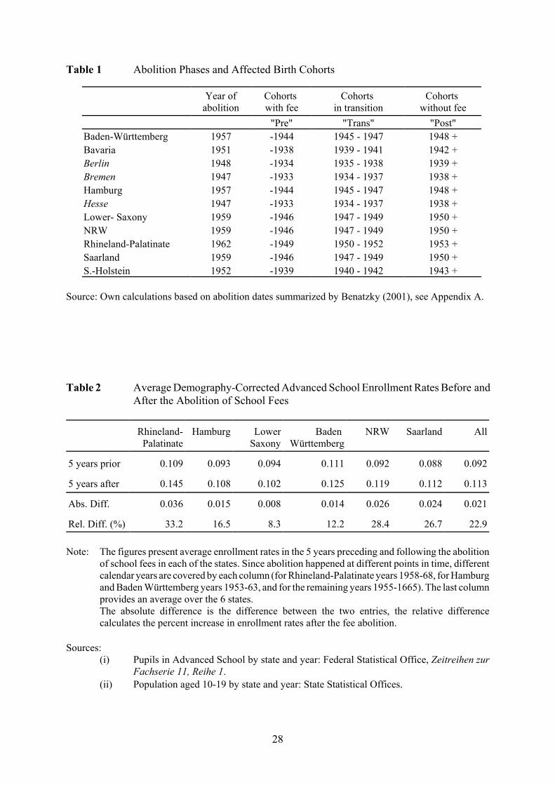
were abolished at different dates for different states, Table 1 indicates the relevant cohort groups

7 Immediately after the war there was some regional experimentation with e.g. longerduration of primary education of 6-8 years prior to the transition into the differentiated tracksystem. This should not affect our analysis. Details are provided in Appendix A.

8 An interesting description of the case of Bavaria is provided by Klafki (1976).

9 Kuhlmann (1970, p.59) provides an illustration of how policy makers thought aboutschool reforms in the 1950s. Reforms were passed based on their alleged educational benefit.Economic cost benefit calculations were not performed. One state secretary of education was infact publicly scolded for raising economic consideration in the discussion of educational reform.

5

for each of the 11 states, Appendix A provides additional explanations.7

In order to convincingly argue that fee abolition helps identify the response of education

demand to changes in education prices we need to establish that the abolition is not jointly

determined with state school enrollment. It is difficult to obtain historic accounts of the political

processes leading to fee abolition.8 However, we can investigate the correlation between the

timing of abolition and state enrollment patterns. Figure 5a depicts Advanced School enrollment

rates for each state's last birth cohort that certainly had to pay fees by the year of fee abolition.

If we account for the general trend to higher enrollment rates over time, the scatter plot hardly

suggests a systematic correlation between the year of abolition and the enrollment rate. A more

likely mechanism determining abolition years might be the political orientation of state

governments: Figure 5a indicates whether the government passing the legislation abolishing fees

was left-wing (SPD) or right-wing (conservative). The evidence is not compelling but suggests

that socialdemocratic governments abolished fees earlier. Figures 5b and 5c present absolute and

relative changes in enrollment rates for the last three birth cohorts unaffected by fee abolition by

year of fee abolition. Again there is no indication of a systematic relationship. Therefore, I

consider the timing of the state-wise abolition of fees as exogenous to state enrollment rates.9

The abolition of school fees was not the only development in the German educational

system during the 1950s and 1960s. Similar to other industrialized countries, the educational

system expanded beginning in the early 1960s. This was due to more sizeable birth cohorts, an

10 The standing conference of state ministers of education agreed in the 1960s to raise thelevel of education and to increase Advanced School enrollment. In consequence, educationexpenditures went up significantly (Fränz and Schulz-Hardt 1998).

11 For the more able it may be possible to earn the highest returns given their education,and they may learn quicker, incurring lower cost of education, e.g. by earning an income at theside, whereas the less able may need additional time and tutoring to meet requirements.

6

increased demand for advanced education, as well as a broadening of access to education with

increasing public investments in the education system.10

2.2 Theoretical Model and Hypotheses

Similar to Card (1999) we model optimal schooling in a framework that abstracts from

dynamic processes and describes the schooling decision as a tradeoff between increases in the

present discounted value of the utility of derived from future earnings, and of the disutility

deriving from education costs. However, we are not interested in the optimal number of years of

schooling but in an individual's (latent) propensity to enrol in Advanced School (S*):

(1) Si* = Y(Si , Ai; :i) - H (Si , Ai, C; <i)

Y is the discounted utility of lifetime earnings and H is the discounted disutility deriving from

Advanced School participation. Both depend on school enrollment (Si) where we would assume

an increasing concave function for Y and an increasing convex function for H. Both may also

vary with a pupil's ability (A), which may yield higher earnings advantages and lower disutility

from additional schooling.11 C represents the direct cost of Advanced School participation

affecting the utility loss due to school participation. :i and <i are person-specific effects.

A simple linear specification of the two factors could be:

(2) Yi = :i + b1 Si + b2 Ai with b1 , b2 > 0

(3) Hi = <i + c1 Si + c2 Ai + C with c1 > 0 and c2 < 0

such that

(4) Si* = ( :i - <i ) + ( b1 - c1 ) Si + ( b2 - c2 ) Ai - C

12 Cawley et al. (1999) provide evidence of higher returns to ability for men comparedto women among whites and hispanics.

7

Clearly, a reduction in C will increase the probability of Advanced School enrollment.

Participation probabilities are higher for the more able students. Also, if e.g. individual effects

:i or returns to schooling and ability (b1, b2) vary systematically across population groups g (with

g=0,1), such as the two sexes, with :g = 1 > :

g = 0 , b1g = 1 > b1

g = 0, or b2g = 1 > b2

g = 0, then it follows that

(5) Si* | g = 1 > Si* | g = 0.

Figure 6 depicts a situation, where pupils are sorted by ability on the abscissa. We expect

that those for whom the expected lifetime benefit of schooling (Yi) exceeds the discounted

disutility (Hi) will attend Advanced School. In Figure 6 everybody to the right of point A will

enrol in Advanced School, here amounting to the 10 percent most able pupils. If fees are

abolished, direct costs (C) decline and the share of pupils in Advanced Schools may increase to

e.g. the 20 percent most able individuals (see point B in Figure 6).

If we hypothesize further, that for parts of the population such as females the expected

benefits at all ability levels are below the average12 - e.g. due to a smaller value of parameter b2 -

then this group's participation share should be below average, both before and after the abolition

of fees. In that case females' Y'i schedule is flatter than males' and females' response to the

abolition of school fees in terms of the relative enrollment increase may exceed that of males (for

details on the theoretical analysis see Appendix B).

Within this framework, the abolition of tuition should cause a decline in the direct cost

of education and yield an overall increase in the participation rate. Given the variation across

federal states and time, we hypothesize:

H1: Advanced School participation increases after the abolition of school fees.H2: Advanced School participation in states without fees exceeds that of states with fees.H3: Advanced School participation for males exceeds that of females.H4: The increase in Advanced School participation may be more pronounced for females than

for males.

13 If, e.g. fees are abolished in Hamburg as of 1957, we would expect higher entry rates(at grade 5) in 1958. However, in 1958 we only know the total number of pupils attendingAdvanced School (grades 5-13).

14 Enrollment rates are calculated as the ratio of the number of pupils in Advanced Schoolin a given state over the total population aged 10-19 in that same state and year.

8

The next sections describe the procedure applied to test these hypotheses.

3. Data Description and Empirical Strategy

3.1 Aggregate Evidence

Our first approach at evaluating the enrollment effects of school fee abolition takes

advantage of historic enrollment data at the state level. Ideally, we would measure the size of the

annual school entry cohorts, but unfortunately only the total number of pupils per year

cumulatively over all 9 grades in Advanced School is available from the state statistical offices.

A disadvantage of this aggregate measure is that changes in school entry can only be measured

to the extent that they change total school enrollment.13 Because of this imprecision in the data

we present average figures across the years before and after the fee abolition. As there were

significant changes in birth cohort sizes in this period we generated demography-corrected

cohort-specific Advanced School enrollment rates by state.14

Since not all of the 11 state statistical offices could provide the necessary figures we are

restricted to evaluate the 6 states described in Table 2. The numbers indicate sizeable increases

in aggregate enrollment rates around the time of the fee abolition. On average the cohort share

attending Advanced School increased by 22.9 percent between the five year periods before and

after the abolition of school fees. This supports Hypothesis 1 (H1), Advanced School

participation increased after the abolition of school fees.

However, this evidence blurs the fee effect by looking at the total number of pupils in

Advanced School and by disregarding the general education expansion over time. For more

9

precise measures and to control for time trends we now turn to individual level data.

3.2 Individual Level Evidence

3.2.1 Data Source and Sample

The individual level data are taken from the Mikrozensus, which is an annual survey of

a one percent random sample of German households. Public use files of 70 percent of the original

data are available for the years 1989, 1991, 1993, 1995, 1996, and 1997. The Mikrozensus uses

a rotating scheme in that the inhabitants of a given dwelling are re-interviewed up to four times.

Unfortunately, households or individuals cannot be identified across survey waves. To avoid a

duplication of records we restrict the analysis to the surveys of 1989, 1993, and 1997 for which

the sets of respondents do not overlap.

Our sample considers the birth cohorts of 1930 through 1959 if they are German nationals

and live in West German states. We drop observations with missing values on key variables such

as age, sex, schooling, or state. This yields a total of 433,315 observations, with about one third

from each of the 3 surveys, and between 10'000 and 18'000 per birth cohort. The key advantage

of the dataset is its size, which allows to compare state-level differences by birth cohort. The

main disadvantage is the lack of social background variables. It would be useful to control for

parental human capital as a determinant of child educational attainment. Given that such

measures are not available, the findings presented below cannot separate the impact of social

background from the measured state and cohort effects. This limitation is addressed in the

discussion below.

3.2.2 Descriptives

Figure 7 describes the development of the enrollment rate in Advanced Schools over

subsequent cohorts. As suggested by Hypothesis 3 (H3) the enrollment rates differ between the

15 The models were also run as linear probability models. While the coefficient signs andsignificances sometimes differed, predictions were in the same direction and at similar ordersof magnitude to those obtained using the logit specification.

10

sexes. They were at about 10 percent for men and 5 percent for women up until the birth cohorts

of the 1930s for which the rates started to increase. For more recent birth cohorts females reach

and even exceed males' educational attainment.

Hypothesis 2 (H2) suggested that enrollment rates in states without fees exceed those in

states with fees for any given cohort. Confirmative evidence is presented in Figure 8, which

depicts average enrollment rates for cohorts in states with and without school fees.

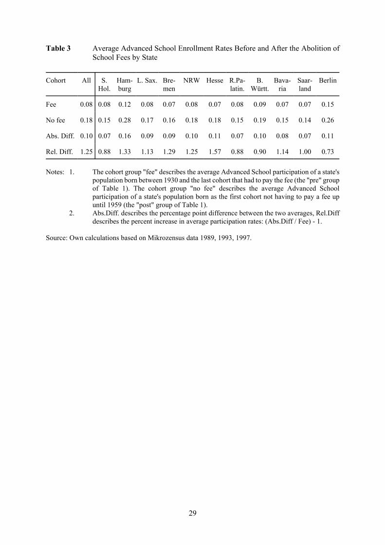
To obtain preliminary evidence on the fee effect, we calculated state-specific Advanced

School participation rates for cohorts entering Advanced School before and after the abolition

of fees. The results in Table 3 yield that on average participation rates increased vastly from 8

percent among the "pre-fee" cohorts to 18 percent for the "post-fee" cohorts. These developments

are similar when calculated for males and females separately. The figures show that not only

levels of education attainment vary across states but also the developments over time are

heterogeneous. We find particularly large increases in Advanced School participation in

Hamburg, and Hesse and the smallest increases in Schleswig-Holstein, and Rhineland-Palatinate.

As these results do not control for time trends we use a regression based strategy next.

3.2.3 Empirical Strategy

The objective of the analysis is to reliably identify the effect of the abolition of school

fees on Advanced School enrollment. Our dependent variable describes whether an individual

obtained an Advanced School degree ("Abitur") and we use a simple logit estimator.15 We apply

four flexible approaches to control for state and period effects.

In Table 1 we categorized the residents of every state in three groups depending on their

year of birth: Those who would have had to pay fees upon entering Advanced School ("pre" fee

11

abolition cohorts), those for whom we cannot be sure ("trans"(itional) birth cohorts), and those

who would not have had to pay fees ("post" fee abolition cohorts). Our four estimation

approaches differ in the flexibility with which they control for time trends and state-specific

effects:

(i) A first approach controls for the cohort groups (pre, trans, post), for state fixed effects,

and a linear cohort effect:

Pr (Si = 1) = 7 (" + $1 transi + $2 posti + ( ci + * State FEi ),

where S indicates Advanced School attendance, 7 represents the logistic cumulative distribution

function, c represents the birth year, trans and post represent cohort group indicators, State FE

stands for a vector of state fixed effects, and ", $, (, and * are coefficients to be determined.

(ii) In order to allow for the possibility that the speed of educational expansion varies

depending on the fee regime in place, a second approach allows for group-specific linear cohort

effects as opposed to one overall linear cohort trend:

Pr (Si = 1) = 7 (" + $1 transi + $2 posti + (1 (prei A ci) + (2 (transi A ci) + (3 (posti A ci)

+ * State FEi ).

(iii) The third approach instead considers state-specific linear cohort trends:

Pr (Si = 1) = 7 (" + $1 transi + $2 posti + (o (State FEi A ci ) + * State FEi ).

(iv) Combining ii and iii, the final approach controls for cohort effects by state and by group:

Pr (Si = 1) = 7 (" + $1 transi + $2 posti + (1o (State FEi A prei A ci)

+ (2o (State FEi A transi A ci) + (3

o (State FEi A posti A ci) + * State FEi ).

The coefficients of the post cohort group indicators ($2) and simulation results inform on

the significance and magnitude of changes in Advanced School attendance after the fee abolition.

Following the recommendations of Bertrand et al. (2004), standard errors are adjusted for clusters

at the state and cohort level.

16 In models 2 and 4 with interaction terms of the cohort group indicators the main effects($1, $2) can of course not be interpreted independently.

17 The results regarding $2 and * hold similarly for estimations that were performedseparately for the two sexes.

18 This simulation procedure involves slight out of sample predictions as the cohorteffects of the pre and the post groups are applied to a person born in the trans group (cf. Table1). The predictions for the full sample are based on the regression results in Table 4. Those forthe gender subsamples are based on separate regressions that are not presented.

19 The standard errors are bootstrapped using 100 repeated draws from the original data.

12

4. Results and Discussion: The Enrollment Effect of Fee Abolition

4.1 Estimation and Simulation Results

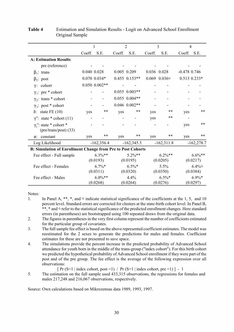
The results of the four estimation approaches discussed above are presented in Panel A

of Table 4. The coefficient estimates for $2 are significant and positive in all specifications

suggesting that the probability of attending Advanced School is higher for individuals who are

not subject to school fees compared to those in the "pre" cohorts.16 The state-specific

heterogeneity in Advanced School enrollment rates is reflected in highly significant state fixed

effects (*).17 In contrast to those in Tables 2 and 3, these results control for aggregate and state-

specific trends reflecting e.g. the educational expansion over time.

Panel B of Table 4 presents the average predicted effect of the abolition of school fees

on Advanced School enrollment probabilities. The hypothetical enrollment probability of an

individual born in the midst of the transition cohort group is compared for the case that she were

to follow the enrollment pattern of the pre-abolition group to the enrollment probability that

would result if she behaved like individuals born in the post-abolition group.18

About representative for subsequent specifications, model (1) yields that the average

enrollment probability increased significantly after the abolition of fees by 6.3 percent for the full

sample.19 Based on separate estimations of model (1) for the two sexes we find a more sizeable

effect of the abolition of fees for females with 6.7 compared to 6.0 percent for males.

20 A test of the specifications in columns (1) and (3) against their more flexiblecounterparts in columns (2) and (4) yields in both cases that the parameter restrictions impliedin specifications (1) and (3) must be rejected at the 1 percent level.

21 For females who start out with an average enrollment rate of about 9 percent before feeabolition the average absolute increase in enrollment rates amounts to 0.6 percentage points, formales starting out with an average enrollment rate of 14.5 percent before fee abolition it amountsto 0.9 percentage points (based on the predictions in specification 1).

13

Adding flexibility to the representation of the time trend, model (2) allows for different

slopes by cohort group: Instead of one time coefficient three interacted effects are estimated.

Their positive coefficients agree with the secular increase in Advanced School enrollment over

time with slower growth for the last cohort group. The predicted fee effects remain within the

range of simulations obtained based on model (1).

Columns (3) and (4) allow for more state-specific flexibility, where the group-cohort

interactions are replaced with eleven state-cohort interaction terms. The predicted overall fee

effect in column (3) of Panel B hardly differs from that in column (1). In model (4) we control

for a separate set of three time trend effects for each of the eleven states yielding 33 parameters

to represent the cohort effects. The predictions still yield an aggregate enrollment increase of 6.6

percent after the abolition of fees.20

The individual level data provides robust evidence for a significant, yet small increase in

the probability of attending Advanced School after the abolition of fees: Starting from an overall

enrollment rate of ten percent (cf. Figure 8) the estimated effect of six percent causes a change

in enrollment rates from about 0.1 to 0.106.21 The effects are small but highly significant.

The outcomes by sex yield mixed evidence: Specifications (1) and (2) suggest a larger

fee effect for females, specifications (3) and (4) yield the reverse. In more restrictive estimations

that impose identical cohort and state effects for both sexes and include a sex main effect and

interactions for the cohort group indicators, we find significantly larger fee abolition effects for

women with a difference of more than 20 percentage points.

22 If, e.g., fees were abolished in Rhineland-Palatinate in 1962, trends for those born inthe 1930s may cause spurious results.

14

4.2 Robustness Tests and Discussion

Next we investigate whether the above results hold up to robustness tests, and discuss

how data limitations might affect the findings.

Sample: One objection to the above analysis may concern the selection of the sample which

includes all observations born between 1930 and 1959. This might cause misleading estimates

of cohort and cohort group effects, as at times irrelevant cohorts are considered, and in some

instances the number of cohorts available to support the estimates is limited.22

To evaluate the effect of such sampling problems the analysis was redone, this time

considering for each state only those 15 cohorts entering Advanced School before and after fee

abolition. The results obtained with this sample are presented in Table 5. We find again

confirmation for increasing enrollment probabilities over time (see the $2 and ( coefficients).

Panel B confirms that the abolition of fees yielded increases in enrollment probabilities: The

simulated effects in specifications (1) and (3) are significantly different from zero at the one

percent level and slightly larger than those in Table 4. On the other hand the predicted effects for

the full sample in specifications (2) and (4) are now reduced in magnitude and statistically

insignificant. Given the significant coefficient estimates and overall positive effects of fee

abolition, our main conclusions are confirmed: There are significant enrollment responses to the

abolition of fees varying between 3 and 7 percent with larger effects for females than for males.

Income Effects: One may argue that the estimation suffers from omitted controls for the

increasing income of the population in post-war Germany. As the speed of economic growth

differed across federal states this may be responsible for the heterogeneity in responses to fee

23 Goldin (1998) finds that higher per capita income at the state level had a strong positiveeffect on secondary schooling in the United States in the early twentieth century.

24 The figures confirm the heterogeneity in state-specific growth processes. WhileBavaria or Schleswig-Holstein quadrupled their real per capita GDP between 1950 and 1980,Bremen or Northrhine-Westphalia merely tripled theirs.

25 We use the value of state-level per capita GDP which was measured in the year whenthe individual turned 11, the typical age of transition to Advanced School.

26 The estimates are not presented to save space and are available upon request.

15

abolition which we noticed in Table 3: inhabitants of poorer states may respond stronger to the

price changes of secondary education.23 To address this problem one would ideally control for

state-specific annual incomes. As an approximation we consider real state-specific per capita

gross domestic product (GDP). Such figures are available annually for West-German states since

1950.24 The GDP information is not available for years prior to 1950, and for Berlin and Saarland

only after 1960. The above estimations were repeated with controls for annual state-level per

capita GDP, where a 'missing-value indicator' was added to the specification for observations

with missing GDP information.25

The estimations with GDP controls yield results that are quite similar to those presented

in Tables 4 and 5.26 The GDP indicators are statistically significant with negative coefficients in

the estimations for the full sample and the male subsample, and insignificant in the female

subsample. This suggests that ceteris paribus the enrollment rate was higher in states with low

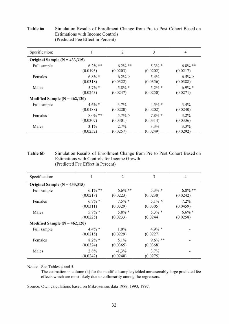
GDP per capita (or missing values). Table 6a summarizes the simulation results obtained for both

samples when GDP controls are added to the models. The fee effects for the original sample are

within the range observed in Table 4 and generally statistically significant. Those for the

modified sample are slightly reduced in size (cf. Table 5). Again, the effects for females are

typically larger than those for men and overall the results seem to be robust to income controls.

Growth Effects: Even though controls for average per capita income do not affect the results,

27 In another experiment we controlled for both income growth and income levels, whichdid not affect the estimated fee abolition effects, either.

28 As model (iv) already considered 33 coefficients, the addition of 33 squared termscaused an overspecification with some unplausibly large coefficient estimates. The simulationsdid not provide informative estimates of the fee effects and are not presented.

16

controls for changes in per capita incomes may well do so. Three arguments support this

presumption: first, when parents consider their children's future earnings potential their

expectations may vary with current and expected future growth rates. Second, parents' liquidity -

as a function of past savings - may be determined by growth rates of the regional economy in

contrast to current income levels. Finally, high growth may also reduce educational investments

because by causing wage raises they increase the opportunity cost of education. To investigate

whether such mechanisms affect our estimates of the fee effect we reestimated our models this

time adding controls for the growth rate of regional per capita GDP instead of its levels.

Simulation results are presented in Table 6b. They yield no important differences compared to

prior results.27

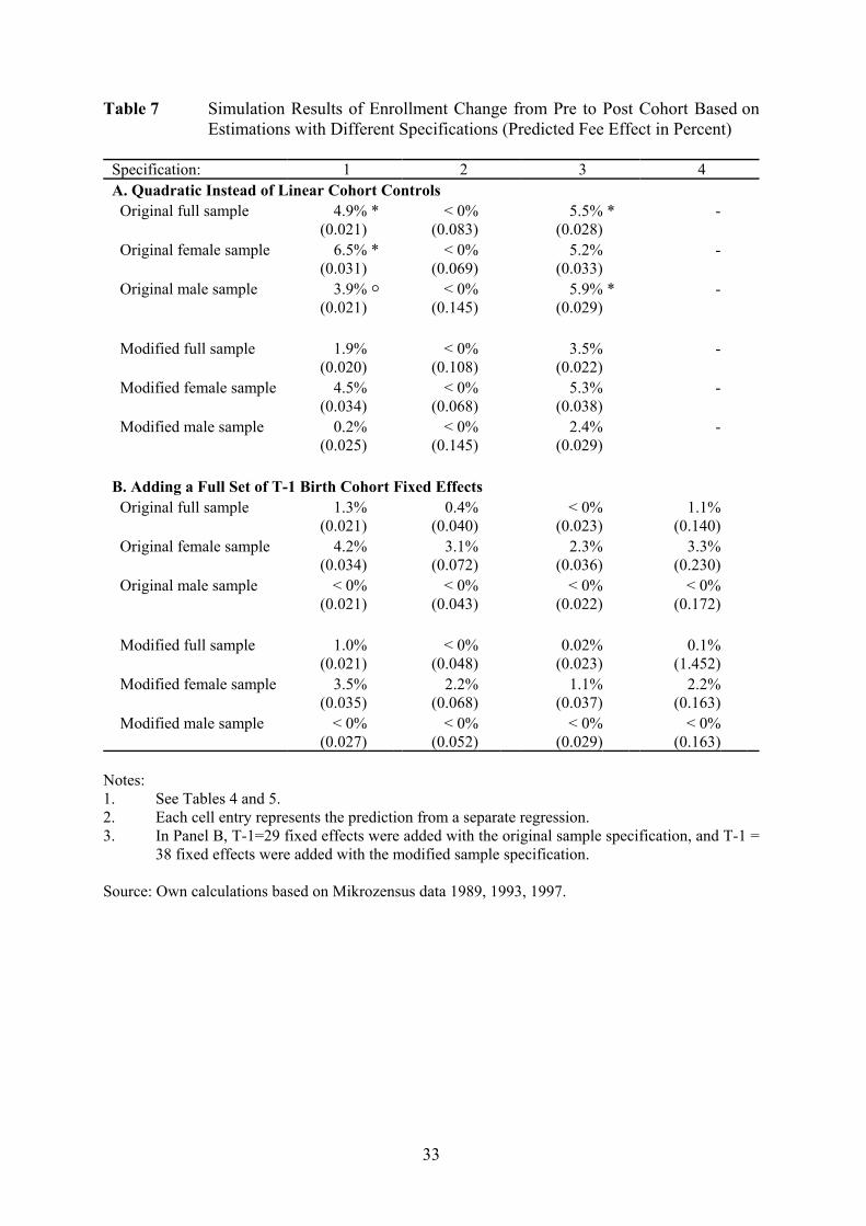
Functional Form Effects: So far we used four linear specifications to control for overall state and

cohort effects. Next, we investigate whether the results are robust to changes in the functional

form of the cohort effects. First, we add quadratic cohort effects (c2) to models (i)-(iii):

(i') Pr (Si = 1 ) = 7 (" + $1 transi + $2 posti + (1 ci + (2 ci2 + * State FEi ),

(ii') Pr (Si = 1) = 7 (" + $1 transi + $2 posti + (1 (prei A ci) + (2 (transi A ci) + (3 (posti A ci)

+ (4 (prei A ci2) + (5 (transi A ci

2) + (6 (posti A ci2) + * State FEi ).

(iii') Pr (Si = 1) = 7 (" + $1 transi + $2 posti + (o1 (State FEi A ci) + (o

2 (State FEi A ci2

)

+ * State FEi )

This generates one additional parameter in specification one, three in specification two, and

eleven in specification three.28 The coefficients of the quadratic cohort effects turn out to be

29 For the original (modified) sample we estimated an additional 29 (38) parameters,which yielded a total of 30, 32, 40, and 62 cohort effect parameters for the four specificationsfor the original sample, and 39, 41,49, and 71 cohort parameters for the modified sample.

17

statistically significant. Panel A of Table 7 describes the simulated fee abolition effects: The fee

effect is still positive and significant in the first and third specifications but negative and always

insignificant in specification (2).

As a second modification of the functional form we add a full vector of birth cohort fixed

effects to the four original specifications.29 These fixed effects are always jointly highly

significant. After adding these rich cohort effects to the previous linear models the predicted fee

abolition effects vanish almost completely. We still find a systematic difference in the effects

obtained for males and females but any remaining fee effect is of small magnitude. We cannot

reject the hypothesis that the fee effects presented before are due to insufficient controls for

overall time trends and year-specific effects in the data. However, the small size of the measured

effects may in part be due to a downward bias that follows from data limitations which we

discuss next.

Enrollment vs. Completion: So far we have not paid much attention to the definition of our

dependent variable, which does not measure Advanced School enrollment but completion of the

Advanced School degree. This could systematically bias the results if the group of individuals

starting Advanced School and the group completing it differ in a way that is correlated with the

effect of school fees. Such a correlation is indeed likely, as the children of better off parents

would be less restricted by school fees and are more likely to receive extra support in completing

their school work compared to children of poor parents. After the abolition of fees more poor kids

might have started Advanced School than show up in our data, which describes only those

successfully completing Advanced School. Therefore, this measurement problem can cause an

30 This underestimation of the true effect is limited by the extent to which children ofpoor parents may be able to balance disadvantages related to their parental background by highereffort or ability. However, Kuhlmann (1970, p.78) shows evidence that the share of pupils withhighly educated parents increases over subsequent grades in Advanced School. This suggeststhat pupils from disadvantaged backgrounds indeed dropped out at faster rates.

18

underestimate of the true enrollment effect of fee abolition, rendering our figures lower bounds.30

Regional Mobility: Since we observe only the state of residence at the time of the survey, we do

not know in which state an individual actually lived when attending school. As long as

individuals moved between states in a random fashion, this would cause an attenuation bias in

the measured effects, again rendering our results lower bounds of the true effect.

An upward bias could result only if migration were correlated with state-specific cohort

group effects, e.g. if individuals with (without) Advanced School degrees moved to states where

they belong to the post (pre) group. We have no evidence confirming such migration patterns.

The German Socioeconomic Panel (GSOEP), an annual household panel survey, provides

evidence on the regional mobility of Germans: every respondent is asked whether he still lives

in the town where he was raised. Living in the same town is obviously more restrictive than

residing in the same state. Nevertheless, in 1985 (2001) 58 (55) percent of the respondents of the

GSOEP sample still lived in the town where they were raised.

As the GSOEP has been in the field for more than 18 years now we can also use the panel

nature of the data to find out that of the (non-representative) sample of 6,284 individuals who

were surveyed both in 1984 and in 2001 only about 5 percent changed their federal state of

residence in between. These figures are indicative of an immobile population. Similar evidence

is provided by Pischke (2003): He shows that about 80 percent of all adult respondents to a large

German social survey still live in their state of birth. Therefore, the effect of neglecting

residential mobility is not likely to be large in magnitude and - unless mobility followed very

specific patterns - it is likely to be uncorrelated with the abolition of school fees. The

31 Specifications 2 and 4 are omitted because the number of "feeyears" is highlycorrelated with the cohort interactions in these models.

19

measurement error may downward bias our estimates.

Anticipation Effects: The abolition of secondary school fees took time: Some states abolished

them early on in their constitutions. Others gave in to the pressure of the occupation forces after

WWII (Furck 1998), while others followed the recommendations of the National Education

Advisory Board, which recommended the abolition of school fees in 1954 (Bohnenkamp et al.

1966). It is possible that we measure only small fee abolition effects because parents changed

their behavior not only when fees were abolished - as we have assumed so far - but much earlier.

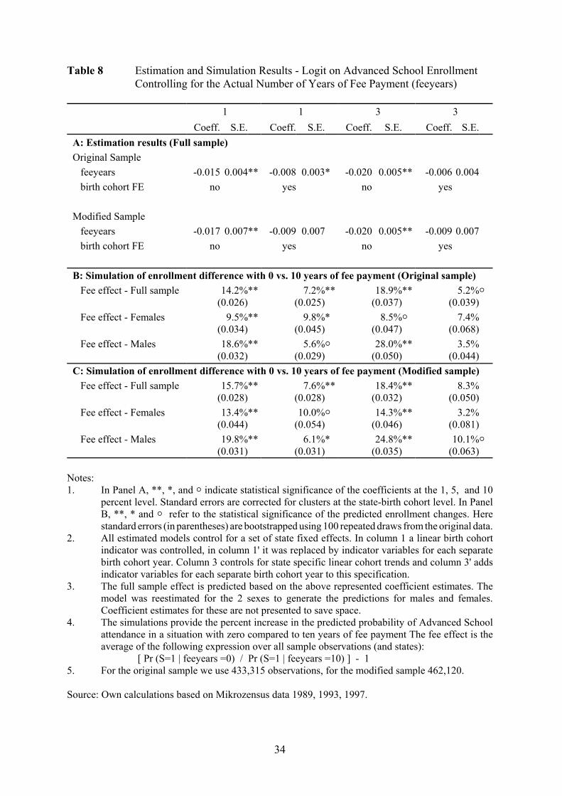
To provide an alternative "benchmark" indicator of the fee effect on enrollment we

investigate whether enrollment probabilities vary with the true number of years that pupils would

have had to pay fees upon enrolling in Advanced School. We modified specifications (1) and (3)

of our model and - in addition to state and cohort effects - controlled for the actual number of

years of fee payment ("feeyears") following Advanced School enrollment.31 This represents a fee

effect under the assumption that parents had perfect foresight. Table 8 presents estimation and

simulation results.

Generally, the number of years during which parents would have had to pay fees yield

a significant negative effect on the probability of child enrollment in Advanced School. The

bottom panel suggests that switching from full fee payment to no fee payment is associated with

increases in the enrollment probabilities at the order of 7 to 8 percent based on the specifications

with cohort fixed effects. Most effects are statistically significant and they are larger for females

than males in specifications controlling for cohort fixed effects. The results support the

conclusion that the abolition of school fees had small but measurable effects on enrollment

probabilities that were larger for females than for males.

32 Kane (1994) shows that a large fraction of the increase in black high school graduationrates in the early 1980s was due to substantial improvements in parental educational background.

33 In that case we would not be able to distinguish between the effects of fee abolition andchanged admission requirements.

20

Omitted Parental Characteristics: The data do not provide information on important covariates

that may influence school attendance decisions, such as parental human capital. This causes a

systematic bias if the omitted parental measures are correlated with the cohort group indicators

(pre, trans, post). Such a correlation is plausible if either the distribution of parental

characteristics or the relevance of the intergenerational transmission of education changed over

time.32 The existing evidence for Germany (see e.g. Blossfeld 1993, Müller and Haun 1993)

suggests that in spite of the educational expansion the intergenerational correlation of educational

success has not changed over time. In addition, there is no reason to expect a large difference in

the level of parental education for those entering Advanced School before and after the fee

abolition, as the educational expansion took place only for cohorts born later than the parents of

the youths considered here. Thus, the omission of parental controls should not substantially affect

the nature of our estimates.

Admission Requirements: Changing admission requirements to Advanced School education over

time may cause shifts in enrollment patterns that interfere with our measures of fee abolition

effects. Unfortunately, there is no source of information on this aspect. Until today admission

standards vary significantly across federal states, with strict grade requirements in southern

Germany and less restrictive systems in other states. Only if these requirements changed exactly

at the time of fee abolition would our estimates be biased.33 However, there does not seem to be

evidence for such developments.

5. Estimation of the Enrollment Sensitivity to Fee Changes

34 Since the full set of relevant state-specific fees is not available, some of the missinginformation on fee amounts was replaced by plausible assumptions. For the state of Saarland weonly know that fees were abolished in 1959. We make no assumptions regarding thedevelopments before 1958 and instead disregard observations from Saarland in this analysis. Theevidence on fee developments is discussed in Benatzky (2001).

21

After the first part of our analyses was devoted to the question of whether the abolition

of fees as such caused behavioral responses in Advanced School enrollment, we now turn to the

price sensitivity of demand for higher secondary education. We regress individual school

enrollment on the fee amounts.34 As the fee amount was set nominally and its real value changed

over time, we deflate the fee measure by calculating the share of the fee per pupil in average

incomes. National average incomes are available from the records of the retirement insurance.

The income share variable represents the state-specific fee-to-income ratio in the year when the

pupils were 11 years of age.

The analysis uses both, the original and the modified sample. The specification of the

school attendance model follows the models described above, only now adding controls for state-

and period-specific income effects (GDP per capita) in all estimations. Since we are no longer

focusing on fee abolition, the cohort group indicators used above are not relevant here. The

models control instead for linear, quadratic, and cubic cohort effects either as main effects or

interacted with state indicators. The estimation results on the original sample are summarized in

Panel A of Table 9.

The estimates yield a clear and generally highly significant negative correlation of the fee-

to-income ratio with individual enrollment probabilities. While the estimated coefficients vary

across specifications, the predicted effect of changes in the fee-to-income ratio on enrollment

rates appears to be rather stable. Panels B and C of Table 9 present the simulated effects of a

decline in the fee-to-income ratio from 10 to 5 percent for the two samples. The simulated effects

are higher when only general cohort controls are considered in the estimations (models 1-3)

compared to the flexible state-specific controls (models 4-6). The predicted enrollment responses

35 In estimations with sex interactions the simulated differences where much larger. Theresults presented in Table 9 are based on separate estimations for the two sexes and are preferredsince they more flexibly capture the sex-specific trend effects.

22

are generally highly significant. A reduction in the fee-to-income ratio by fifty percent is

correlated with enrollment increases at the order of about 3 percent for the full sample with

somewhat larger effects for the female subsample.35 This result matches the 6 percent average

enrollment effect predicted for fee abolition (i.e. reduction by 100 percent) surprisingly well.

6. Discussion and Conclusions

In times of tight public budgets changes in school fees and tuition are intensely debated.

Informed political decisions must be based on evidence regarding the price sensitivity of

education demand which is difficult to obtain. This study takes advantage of a natural experiment

to measure the effect of school fees on enrollment: In post-WWII West Germany, fees for

advanced secondary schools were abolished at different points in time between 1947 and 1962

across eleven federal states. The variation across time and state is used to identify the fee effect.

Based on a variant of Card's (1999) optimal schooling model, we derive four hypotheses

on the enrollment effect of school fees. Overall, our evidence is consistent with the hypotheses

that Advanced School participation (1) increases after the abolition of fees, (2) is higher in states

without fees than in states with fees, (3) among males exceeds that among females, and (4)

increases more for females than for males following the fee abolition.

Aggregate data suggest sizeable enrollment increases around the period of fee abolition.

When we control for overall time trends using individual level data we find significant increases

in Advanced School enrollment at the time of the abolition of fees at the order of 6 percent with

larger effects for females than for males. Similarly, a reduction in the fee-to-income ratio by 50

percent is associated with an increase in the enrollment rates of about 3 percent, with a higher

36 In terms of current incomes the simulated fee change (five percent of annual incomes)would be equivalent to a nominal change in fees by i 1400 (or $ 1700) per year.

23

price elasticity for girls' than for boys' education.36

There are two important limitations to these results: On the one hand they may

underestimate the true effect of fee abolition because our data are subject to measurement error

relating to the exact definition of school enrollment and to individuals' state of residence in their

youth. On the other hand the results are not completely robust to changes in specification. While

they hold up to different definitions of the relevant sample, to four increasingly flexible models

which are linear in cohort effects, and some models which allow for quadratic cohort effects, the

predicted effects diminish in magnitude or vanish when rich birth cohort fixed effects are added

to the specifications. Even though some of these specifications yield significant small positive

effects of the abolition of school fees on enrollment, the most flexible specifications do not allow

us to reject the null hypothesis of zero enrollment effects of fee abolition.

This result might be affected by the attenuation bias following from measurement error

in our explanatory variables or from systematic noise in the dependent variable. Substantively,

the small effect may have a number of reasons: It might reflect that demand for education was

indeed price inelastic or that the fee amount was too small to yield more sizeable responses.

Küchenhoff (1952) and Bergmann (1955) point out that even after tuition fees were abolished

certain other education related payments (examination fees, certification fees, accident insurance

premia) were still collected and Advanced School fees only reflected a small part of the total

expenses related to this type of schooling.

Alternatively, the small magnitude of the measured effect might be due to the protracted

abolition of fees, where parents expected that fees were to be abolished and thus adjusted their

behavior over longer periods then assumed here. Also, the change in fees may have followed a

change in parental tastes for education such that the price elasticity of demand had changed (e.g.

24

due to social developments) even before fees were abolished. This would be a variant of an

anticipation effect.

Capacity constraints may be responsible for the small demand response to fee abolition,

as well: immediately after the war there was a major shortage of buildings for all types of

schools. Kuhlmann (1970 p.27) suggests that through the mid 1950s insufficient school capacity

was an acknowledged limitation to educational expansion: the National Education Advisory

Board recommended in 1954 that school fees ought to be abolished but not at the expense of the

solution of more urgent problems such as the provision school buildings (Bohnenkamp et al.

1966). If schools could not accommodate pupils we may not be able to measure demand effects.

Finally, it may be that those able pupils for whom school fees would have been

prohibitive had always been supported on the basis of individual scholarships. If such systems

were successful in promoting the brightest poor this would clearly reduce the measurable effect

of the fee abolition. While such support systems existed, their overriding effectiveness is

questionable. Küchenhoff (1955) discusses that only between one and two percent of the pupils

in Advanced Schools were supported by public funds and that scholarships were available only

for university students.

In sum, our results suggest that the existence of school fees for Advanced Schools set a

small but measurable barrier to higher education which affected females more than males. The

differential price sensitivity for male and female students may provide part of the answer to the

question why even today one finds significant enrollment differences between the sexes for

higher education: Parental demand for girls' education seems to be more price elastic. Finally,

given the limited size of the measured effects, the existence of school fees hardly explains the

differential developments of secondary school graduation rates during the early decades of the

twentieth century in Germany and the United States.

25

References

Aakvik, Arild, Kjell G. Salvanes, Kjell Vaage, 2003, Measuring Heterogeneity in the Returns toEducation in Norway Using Educational Reforms, CEPR Discussion Paper No. 4088.

Benatzky, Joachim, 2001, Dokumentation Schulgeld in Deutschland, mimeo, University of Mainz.

Berger, Daniel J. and Christoph Ehmann, 2000, Gebühren für Bildung - ein Anschlag auf dieChancengleichheit? Auswirkungen der Abschaffung und die Erhebung von Gebühren imdeutschen Bildungswesen, Recht der Jugend und des Bildungswesens 48(4), 356-376.

Bergmann, Bernhard, 1955, Schulgeldfreiheit und soziale Begabtenförderung, Pädagogische Rundschau10, 178-183.

Bertrand, Marianne, Esther Duflo, and Sendhil Mullainathan, 2004, How much should we trustdifference-in-differences estimates?, Quarterly Journal of Economics 119(1), 249-275.

Blossfeld, Hans-Peter, 1993, Changes in the Educational Opportunities in the Federal Republic ofGermany. A Longitudinal Study of Cohorts Born Between 1916 and 1965, in: Blossfeld, Hans-Peter and Yossi Shavit (eds.), Persistent Inequality: Changing Educational Stratification in 13Countries, Westview Press, Boulder CO, 51-74.

Bohnenkamp, Hans, Walter Dirks, Doris Knab, 1966, Empfehlungen und Gutachten des DeutschenAusschusses für das Erziehungs- und Bildungswesen 1953-1965. Gesamtausgabe, Ernst KlettVerlag, Stuttgart.

Card, David, 1999, The Causal Effect of Education on Earnings, in: Ashenfelter O. and D. Card (eds.)Handbook of Labor Economics Vol. 3 Chapter 30, Elsevier Science B.V., 1801-1863.

Cawley, John, James Heckman, and Edward Vytlacil, 1999, Meritocracy in America: Wages Within andAcross Occuptions, Industrial Relations 38(3), 250-296.

Dearden, Lorraine, Carl Emmerson, Christine Frayen, and Costas Meghir, 2003, The Impact of FinancialIncentives on Education Choice, mimeo, Institute for Fiscal Studies, London.

Dynarski, Susan, 2002, The Behavioral and Distributional Implications of Aid for College, AmericanEconomic Review 92(2), 279-285.

Epple, Dennis and Richard Romano, 1998, Competition between private and public schools, vouchers,and peer group effects, American Economic Review 88(1), 33-62.

Epple, Dennis, David Figlio, and Richard Romano, 2004, Competition between private and publicschools: testing stratification and pricing predictions, Journal of Public Economics 88(7-8), 1215-1245.

Fränz, Peter and Joachim Schulz-Hardt, 1998, Zur Geschichte der Kultusministerkonferenz 1948 - 1998,in: Sekretariat der Kultusministerkonferenz (ed.), Einheit in der Vielfalt. 50 JahreKultusministerkonferenz 1948 - 1998, Neuwied et al., Luchterhand, 177-227.

Furck, Carl-Ludwig, 1998, Allgemeinbildende Schulen: Entwicklungstendenzen und Rahmen-bedingungen, in: Führ, Christoph and Carl-Ludwig Furck (eds.), Handbuch der deutschenBildungsgeschichte Band VI: 1945 bis zur Gegenwart, Verlag C.H. Beck, Munich, 245-260.

26

Geissler, Gert, 2000, Geschichte des Schulwesens in der Sowjetischen Besatzungszone und in derDeutschen Demokratischen Republik 1945 bis 1962, Lang, Frankfurt/Main.

Goldin, Claudia, 1998, America's Graduation from High School: The Evolution and Spread of SecondarySchooling in the Twentieth Century, Journal of Economic History 58(2), 345-374.

Goldin, Claudia and Lawrence C. Katz, 1997, Why the United States Led in Education: Lessons fromSecondary School Expansion, 1910 to 1940, National Bureau of Economic Research WorkingPaper No. 6144.

Goldin, Claudia and Lawrence C. Katz, 2003, Mass Secondary Schooling and the State: The Role of StateCompulsion in the High School Movement, National Bureau of Economic Research WorkingPaper No. 10075.

Heckman, James J., Lance Lochner, and Christopher Taber, 1998, General-Equilibrium Treatment Effects:A Study of Tuition Policy, American Economic Review 88(2), 381-386.

Ichimura, Hidehiko and Christopher Taber, 2002, Semiparametric Reduced-Form Estimation of tuitionSubsidies, American Economic Review 92(2), 286-292.

Ichino, Andrea and Rudolf Winter-Ebmer, 2004, The Long-Run Educational Cost of World War II,Journal of Labor Economics 22(1), 57-86.

Kahlert, Helmut, 1974, Das Schulgeld als Instrument der Finanz- und Bildungspolitik, Recht der Jugendund des Bildungswesens 22, 38-44.

Kane, Thomas J., 1994, College Entry by Blacks since 1970: The Role of College Costs, FamilyBackground, and the Returns to Education, Journal of Political Economy 102(5), 878-911.

Kane, Thomas J., 1995, Rising Public College Tuition and College Entry: How well do Public SubsidiesPromote Access to College, NBER Working Paper No. 5164.

Kim, Jooseop, Harold Alderman, and Peter F. Orazem, 1999, Can Private Subsidies Increase Enrolmentfor the Poor? The Quetta Urban Fellowship Program, World Bank Economic Review 13(3), 443-465.

Klafki, Wolfgang, 1976, Aspekte kritisch-konstruktiver Erziehungswissenschaft, Beltz Verlag, Weinheimand Basel.

Küchenhoff, Werner, 1952, Schulgeld und Begabtenförderung in der Bundesrepublik, Sozialer Fortschritt1, 92-94.

Küchenhoff, Werner, 1955, Schulgeld und Begabtenförderung in der Bundesrepublik, Sozialer Fortschritt4, 135-136.

Kuhlmann, Caspar, 1970, Schulreform und Gesellschaft in der Bundesrepublik Deutschland 1946-1966,Ernst Klett Verlag, Stuttgart.

Ladd, Helen F., 2002, School Vouchers: A Critical View, Journal of Economic Perspectives 16(4), 3-24.

Miguel, Edward and Michael Kremer, 2004, Worms: Identifying Impacts on Education and Health in thePresence of Treatment Externalities, Econometrica 72(1), 159-217.

27

Meghir, Costas and Marten Palme, 2003, Ability, Parental Background, and Education Policy: EmpiricalEvidence from a Social Experiment, Institute for Fiscal Studies Working Paper 03/05, London.

Müller, Werner and D. Haun, 1993, Bildungsgleichheit im sozialen Wandel, Kölner Zeitschrift fürSoziologie und Sozialpsychologie 46, 1-46.

Neal, Derek, 2002, How Vouchers Could Change the Market for Education, Journal of EconomicPerspectives 16(4), 25-44.

Pischke, Jörn-Steffen, 2003, The Impact of Length of the School Year on Student Performance andEarnings: Evidence from the German Short School Years, CEPR Discussion Paper No. 4074.

Schultz, T. Paul, 2000, Final Report: The Impact of Progesa on School Enrollments, mimeo, InternationalFood Policy Research Institute, Washington D.C.

Vermeersch, Christel, 2002, School Meals, Educational Achievement and School Competition: Evidencefrom a Randomized Evaluation, mimeo, Harvard University.

28

Table 1 Abolition Phases and Affected Birth Cohorts

Year ofabolition

Cohorts with fee

Cohorts in transition

Cohorts without fee

"Pre" "Trans" "Post"Baden-Württemberg 1957 -1944 1945 - 1947 1948 +Bavaria 1951 -1938 1939 - 1941 1942 +Berlin 1948 -1934 1935 - 1938 1939 +Bremen 1947 -1933 1934 - 1937 1938 +Hamburg 1957 -1944 1945 - 1947 1948 +Hesse 1947 -1933 1934 - 1937 1938 +Lower- Saxony 1959 -1946 1947 - 1949 1950 +NRW 1959 -1946 1947 - 1949 1950 +Rhineland-Palatinate 1962 -1949 1950 - 1952 1953 +Saarland 1959 -1946 1947 - 1949 1950 +S.-Holstein 1952 -1939 1940 - 1942 1943 +

Source: Own calculations based on abolition dates summarized by Benatzky (2001), see Appendix A.

Table 2 Average Demography-Corrected Advanced School Enrollment Rates Before andAfter the Abolition of School Fees

Rhineland-Palatinate

Hamburg LowerSaxony

Baden Württemberg

NRW Saarland All

5 years prior 0.109 0.093 0.094 0.111 0.092 0.088 0.092

5 years after 0.145 0.108 0.102 0.125 0.119 0.112 0.113

Abs. Diff. 0.036 0.015 0.008 0.014 0.026 0.024 0.021

Rel. Diff. (%) 33.2 16.5 8.3 12.2 28.4 26.7 22.9

Note: The figures present average enrollment rates in the 5 years preceding and following the abolitionof school fees in each of the states. Since abolition happened at different points in time, differentcalendar years are covered by each column (for Rhineland-Palatinate years 1958-68, for Hamburgand Baden Württemberg years 1953-63, and for the remaining years 1955-1665). The last columnprovides an average over the 6 states. The absolute difference is the difference between the two entries, the relative differencecalculates the percent increase in enrollment rates after the fee abolition.

Sources:(i) Pupils in Advanced School by state and year: Federal Statistical Office, Zeitreihen zur

Fachserie 11, Reihe 1.(ii) Population aged 10-19 by state and year: State Statistical Offices.

29

Table 3 Average Advanced School Enrollment Rates Before and After the Abolition ofSchool Fees by State

Cohort All S.Hol.

Ham-burg

L. Sax. Bre-men

NRW Hesse R.Pa-latin.

B.Württ.

Bava-ria

Saar-land

Berlin

Fee 0.08 0.08 0.12 0.08 0.07 0.08 0.07 0.08 0.09 0.07 0.07 0.15

No fee 0.18 0.15 0.28 0.17 0.16 0.18 0.18 0.15 0.19 0.15 0.14 0.26

Abs. Diff. 0.10 0.07 0.16 0.09 0.09 0.10 0.11 0.07 0.10 0.08 0.07 0.11

Rel. Diff. 1.25 0.88 1.33 1.13 1.29 1.25 1.57 0.88 0.90 1.14 1.00 0.73

Notes: 1. The cohort group "fee" describes the average Advanced School participation of a state'spopulation born between 1930 and the last cohort that had to pay the fee (the "pre" groupof Table 1). The cohort group "no fee" describes the average Advanced Schoolparticipation of a state's population born as the first cohort not having to pay a fee upuntil 1959 (the "post" group of Table 1).

2. Abs.Diff. describes the percentage point difference between the two averages, Rel.Diffdescribes the percent increase in average participation rates: (Abs.Diff / Fee) - 1.

Source: Own calculations based on Mikrozensus data 1989, 1993, 1997.

30

Table 4 Estimation and Simulation Results - Logit on Advanced School EnrollmentOriginal Sample

1 2 3 4Coeff. S.E. Coeff. S.E. Coeff. S.E. Coeff. S.E.

A: Estimation Results pre (reference) - - - - - - - - $1: trans 0.040 0.028 0.005 0.209 0.036 0.028 -0.478 0.746 $2: post 0.070 0.034* 0.455 0.153** 0.069 0.036N 0.513 0.233* (: cohort 0.050 0.002** - - - - - - (1: pre * cohort - - 0.055 0.003** - - - - (2: trans * cohort - - 0.055 0.004** - - - - (3: post * cohort - - 0.046 0.002** - - - - *: state FE (10) yes ** yes ** yes ** yes ** (o: state * cohort (11) - - - - yes ** - (j

o: state * cohort * (pre/trans/post) (33)

- - - - - - yes **

": constant yes ** yes ** yes ** yes ** Log Likelihood -162,356.4 -162,345.5 -162,311.8 -162,278.7B: Simulation of Enrollment Change from Pre to Post Cohorts Fee effect - Full sample 6.3%

(0.0193)** 5.2%

(0.0195)** 6.2%

(0.0205)** 6.6%

(0.0217)**

Fee effect - Females 6.7%(0.0311)

* 6.5%(0.0320)

* 5.5%(0.0350)

6.4%(0.0384)

N

Fee effect - Males 6.0%(0.0268)

** 4.4%(0.0264)

6.5%(0.0276)

* 6.9%(0.0297)

*

Notes:1. In Panel A, **, *, and N indicate statistical significance of the coefficients at the 1, 5, and 10

percent level. Standard errors are corrected for clusters at the state-birth cohort level. In Panel B,**, * and N refer to the statistical significance of the predicted enrollment changes. Here standarderrors (in parentheses) are bootstrapped using 100 repeated draws from the original data.

2. The figures in parentheses in the very first column represent the number of coefficients estimatedfor the particular group of covariates.

3. The full sample fee effect is based on the above represented coefficient estimates. The model wasreestimated for the 2 sexes to generate the predictions for males and females. Coefficientestimates for these are not presented to save space.

4. The simulations provide the percent increase in the predicted probability of Advanced Schoolattendance for youth born in the middle of the trans-group ("index cohort"). For this birth cohortwe predicted the hypothetical probability of Advanced School enrollment if they were part of thepost and of the pre group. The fee effect is the average of the following expression over allobservations:

[ Pr (S=1 | index cohort, post =1) / Pr (S=1 | index cohort, pre =1) ] - 15. The estimation on the full sample used 433,315 observations, the regressions for females and

males 217,248 and 216,067 observations, respectively.

Source: Own calculations based on Mikrozensus data 1989, 1993, 1997.

31

Table 5 Estimation and Simulation Results - Logit on Advanced School EnrollmentModified Sample

1 2 3 4Coeff. S.E. Coeff. S.E. Coeff. S.E. Coeff. S.E.

A: Estimation Results pre (reference) - - - - - - - - $1: trans 0.044 0.028 0.073 0.208 0.054 0.028* -0.105 0.767 $2: post 0.072 0.036* 0.557 0.135** 0.080 0.034* 0.786 0.159** (: cohort 0.049 0.002** - - - - - - (1: pre * cohort - - 0.059 0.003** - - - - (2: trans * cohort - - 0.057 0.004** - - - - (3: post * cohort - - 0.047 0.002** - - - - *: state FE (10) yes ** yes ** yes ** yes ** (o: state * cohort (11) - - - - yes ** - (j

o: state * cohort * (pre/trans/post) (33)

- - - - - - yes **

": constant yes ** yes ** yes ** yes ** Log Likelihood -182,581.3 -182,561.94 -182,516.78 -182.471.52B: Simulation of Enrollment Change from Pre to Post Cohorts Fee effect - Full sample 6.5%

(0.0161)** 2.7%

(0.0195)7.3%

(0.0205)** 2.7%

(0.0217) Fee effect - Females 8.4%

(0.0377)* 5.8%

(0.0392)8.8%

(0.0385)* 3.4%

(0.0404) Fee effect - Males 6.4%

(0.0266)* 1.0%

(0.0275)7.3%

(0.0276)** 2.3%

(0.0301)

Notes:1. In Panel A, **, *, and N indicate statistical significance of the coefficients at the 1, 5, and 10

percent level. Standard errors are corrected for clusters at the state-birth cohort level. In PanelB, **, * and N refer to the statistical significance of the predicted enrollment changes. Herestandard errors (in parentheses) are bootstrapped using 100 repeated draws from the original data.

2. The figures in parentheses in the very first column represent the number of coefficients estimatedfor the particular group of covariates.

3. The full sample fee effect is based on the above represented coefficient estimates. The model wasreestimated for the 2 sexes to generate the predictions for males and females. Coefficientestimates for these are not presented to save space.

4. The simulations provide the percent increase in the predicted probability of Advanced Schoolattendance for youth born in the middle of the trans-group ("index cohort"). For this birth cohortwe predicted the hypothetical probability of Advanced School enrollment if they were part of thepost and of the pre group. The fee effect is the average of the following expression over allobservations:

[ Pr (S=1 | index cohort, post =1) / Pr (S=1 | index cohort, pre =1) ] - 15. The estimation on the full sample used 462,120 observations, the regressions for females and

males 231,247 and 230,873 observations, respectively.

Source: Own calculations based on Mikrozensus data 1989, 1993, 1997.

32

Table 6a Simulation Results of Enrollment Change from Pre to Post Cohort Based onEstimations with Income Controls(Predicted Fee Effect in Percent)

Specification: 1 2 3 4

Original Sample (N = 433,315) Full sample 6.2%

(0.0193)** 6.2%

(0.0203)** 5.3%

(0.0202)* 6.8%

(0.0217)**

Females 6.8%(0.0318)

* 6.2%(0.0322)

N 5.4%(0.0356)

6.5%(0.0388)

N

Males 5.7%(0.0243)

* 5.8%(0.0247)

* 5.2%(0.0250)

* 6.9%(0.0271)

*

Modified Sample (N = 462,120) Full sample 4.6%

(0.0188)* 3.7%

(0.0220)4.5%

(0.0202)* 3.4%

(0.0240) Females 8.0%

(0.0307)** 5.7%

(0.0301)N 7.8%

(0.0314)* 3.2%

(0.0336) Males 3.1%

(0.0252)2.7%

(0.0257)3.3%

(0.0249)3.3%

(0.0292)

Table 6b Simulation Results of Enrollment Change from Pre to Post Cohort Based onEstimations with Controls for Income Growth(Predicted Fee Effect in Percent)

Specification: 1 2 3 4

Original Sample (N = 433,315) Full sample 6.1%

(0.0218)** 6.6%

(0.0223)** 5.3%

(0.0230)* 6.8%

(0.0242)**

Females 6.7%(0.0311)

* 7.5%(0.0329)

* 5.1%(0.0305)

N 7.2%(0.0459)

Males 5.7%(0.0225)

* 5.8%(0.0233)

* 5.3%(0.0244)

* 6.6%(0.0258)

*

Modified Sample (N = 462,120) Full sample 4.4%

(0.0215)* 1.0%

(0.0229)4.9%

(0.0227)* -

Females 8.2%(0.0324)

* 5.1%(0.0365)

9.6%(0.0368)

** -

Males 2.8%(0.0242)

-1,3%(0.0240)

3.7%(0.0275)

-

Notes: See Tables 4 and 5.The estimation in column (4) for the modified sample yielded unreasonably large predicted feeeffects which are most likely due to collinearity among the regressors.

Source: Own calculations based on Mikrozensus data 1989, 1993, 1997.

33

Table 7 Simulation Results of Enrollment Change from Pre to Post Cohort Based onEstimations with Different Specifications (Predicted Fee Effect in Percent)

Specification: 1 2 3 4A. Quadratic Instead of Linear Cohort Controls Original full sample 4.9%

(0.021)* < 0%

(0.083)5.5%

(0.028)* -

Original female sample 6.5%(0.031)

* < 0%(0.069)

5.2%(0.033)

-

Original male sample 3.9%(0.021)

N < 0%(0.145)

5.9%(0.029)

* -

Modified full sample 1.9%(0.020)

< 0%(0.108)

3.5%(0.022)

-

Modified female sample 4.5%(0.034)

< 0%(0.068)

5.3%(0.038)

-

Modified male sample 0.2%(0.025)

< 0%(0.145)

2.4%(0.029)

-

B. Adding a Full Set of T-1 Birth Cohort Fixed Effects Original full sample 1.3%

(0.021)0.4%

(0.040)< 0%

(0.023)1.1%

(0.140) Original female sample 4.2%

(0.034)3.1%

(0.072)2.3%

(0.036)3.3%

(0.230) Original male sample < 0%

(0.021)< 0%

(0.043)< 0%

(0.022)< 0%

(0.172)

Modified full sample 1.0%(0.021)

< 0%(0.048)

0.02%(0.023)

0.1%(1.452)

Modified female sample 3.5%(0.035)

2.2%(0.068)

1.1%(0.037)

2.2%(0.163)

Modified male sample < 0%(0.027)

< 0%(0.052)

< 0%(0.029)

< 0%(0.163)

Notes: 1. See Tables 4 and 5.2. Each cell entry represents the prediction from a separate regression. 3. In Panel B, T-1=29 fixed effects were added with the original sample specification, and T-1 =

38 fixed effects were added with the modified sample specification.

Source: Own calculations based on Mikrozensus data 1989, 1993, 1997.

34

Table 8 Estimation and Simulation Results - Logit on Advanced School EnrollmentControlling for the Actual Number of Years of Fee Payment (feeyears)

1 1 3 3Coeff. S.E. Coeff. S.E. Coeff. S.E. Coeff. S.E.

A: Estimation results (Full sample)Original Sample feeyears -0.015 0.004** -0.008 0.003* -0.020 0.005** -0.006 0.004 birth cohort FE no yes no yes

Modified Sample feeyears -0.017 0.007** -0.009 0.007 -0.020 0.005** -0.009 0.007 birth cohort FE no yes no yes

B: Simulation of enrollment difference with 0 vs. 10 years of fee payment (Original sample) Fee effect - Full sample 14.2%

(0.026)** 7.2%

(0.025)** 18.9%

(0.037)** 5.2%

(0.039)N

Fee effect - Females 9.5%(0.034)

** 9.8%(0.045)

* 8.5%(0.047)

N 7.4%(0.068)

Fee effect - Males 18.6%(0.032)

** 5.6%(0.029)

N 28.0%(0.050)

** 3.5%(0.044)

C: Simulation of enrollment difference with 0 vs. 10 years of fee payment (Modified sample) Fee effect - Full sample 15.7%

(0.028)** 7.6%

(0.028)** 18.4%

(0.032)** 8.3%

(0.050) Fee effect - Females 13.4%

(0.044)** 10.0%

(0.054)N 14.3%

(0.046)** 3.2%

(0.081) Fee effect - Males 19.8%

(0.031)** 6.1%

(0.031)* 24.8%

(0.035)** 10.1%

(0.063)N

Notes:1. In Panel A, **, *, and N indicate statistical significance of the coefficients at the 1, 5, and 10

percent level. Standard errors are corrected for clusters at the state-birth cohort level. In PanelB, **, * and N refer to the statistical significance of the predicted enrollment changes. Herestandard errors (in parentheses) are bootstrapped using 100 repeated draws from the original data.

2. All estimated models control for a set of state fixed effects. In column 1 a linear birth cohortindicator was controlled, in column 1' it was replaced by indicator variables for each separatebirth cohort year. Column 3 controls for state specific linear cohort trends and column 3' addsindicator variables for each separate birth cohort year to this specification.

3. The full sample effect is predicted based on the above represented coefficient estimates. Themodel was reestimated for the 2 sexes to generate the predictions for males and females.Coefficient estimates for these are not presented to save space.

4. The simulations provide the percent increase in the predicted probability of Advanced Schoolattendance in a situation with zero compared to ten years of fee payment The fee effect is theaverage of the following expression over all sample observations (and states):

[ Pr (S=1 | feeyears =0) / Pr (S=1 | feeyears =10) ] - 15. For the original sample we use 433,315 observations, for the modified sample 462,120.

Source: Own calculations based on Mikrozensus data 1989, 1993, 1997.

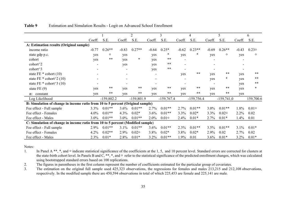
35

Table 9 Estimation and Simulation Results - Logit on Advanced School Enrollment

1 2 3 4 5 6Coeff. S.E. Coeff. S.E. Coeff. S.E. Coeff. S.E. Coeff. S.E. Coeff. S.E.

A: Estimation results (Original sample) income ratio -0.77 0.26** -0.83 0.27** -0.64 0.25* -0.62 0.23** -0.69 0.26** -0.43 0.23N state gdp p.c. yes N yes yes * yes * yes N yes N cohort yes ** yes * yes ** - - - cohort^2 - yes yes ** - - - cohort^3 - - yes ** - - - state FE * cohort (10) - - - yes ** yes ** yes ** state FE * cohort^2 (10) - - - - yes * yes ** state FE * cohort^3 (10) - - - - - yes ** state FE (9) yes ** yes ** yes ** yes ** yes ** yes * ": constant yes ** yes ** yes ** yes ** yes ** yes Log Likelihood -159,802.2 -159,801.9 -159,767.4 -159,756.4 -159,741,0 159,700.6B: Simulation of change in income ratio from 10 to 5 percent (Original sample)Fee effect - Full sample 3.3% 0.01** 3.6% 0.01** 2.7% 0.01** 2.7% 0.01** 3.0% 0.01** 1.8% 0.01NFee effect - Females 4.0% 0.01** 4.3% 0.02* 3.6% 0.01** 3.3% 0.02* 3.3% 0.02N 2.2% 0.02Fee effect - Males 3.0% 0.01** 3.0% 0.01** 2.0% 0.01N 2.4% 0.01* 2.7% 0.01* 1.4% 0.01 C: Simulation of change in income ratio from 10 to 5 percent (Modified sample)Fee effect - Full sample 2.9% 0.01** 3.1% 0.01** 3.6% 0.01** 2.3% 0.01** 3.5% 0.01** 3.1% 0.01* Fee effect - Females 4.2% 0.02** 2.9% 0.02N 3.8% 0.02* 3.8% 0.02* 2.9% 0.02 2.7% 0.02Fee effect - Males 2.3% 0.01* 2.8% 0.01* 3.2% 0.01** 1.9% 0.01 3.6% 0.01* 3.2% 0.01*

Notes:1. In Panel A **, *, and N indicate statistical significance of the coefficients at the 1, 5, and 10 percent level. Standard errors are corrected for clusters at

the state-birth cohort level. In Panels B and C, **, *, and N refer to the statistical significance of the predicted enrollment changes, which was calculatedusing bootstrapped standard errors based on 100 replications.

2. The figures in parentheses in the first column represent the number of coefficients estimated for the particular group of covariates. 3. The estimation on the original full sample used 425,323 observations, the regressions for females and males 213,215 and 212,108 observations,

respectively. In the modified sample there are 450,594 observations in total of which 225,453 are female and 225,141 are male.

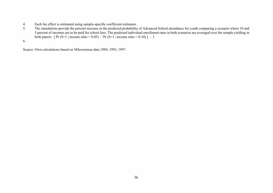
36

4. Each fee effect is estimated using sample-specific coefficient estimates.5. The simulations provide the percent increase in the predicted probability of Advanced School attendance for youth comparing a scenario where 10 and

5 percent of incomes are to be paid for school fees. The predicted individual enrollment rates in both scenarios are averaged over the sample yielding inboth panels: [ Pr (S=1 | income ratio = 0.05) / Pr (S=1 | income ratio = 0.10) ] - 1

6.

Source: Own calculations based on Mikrozensus data 1989, 1993, 1997.

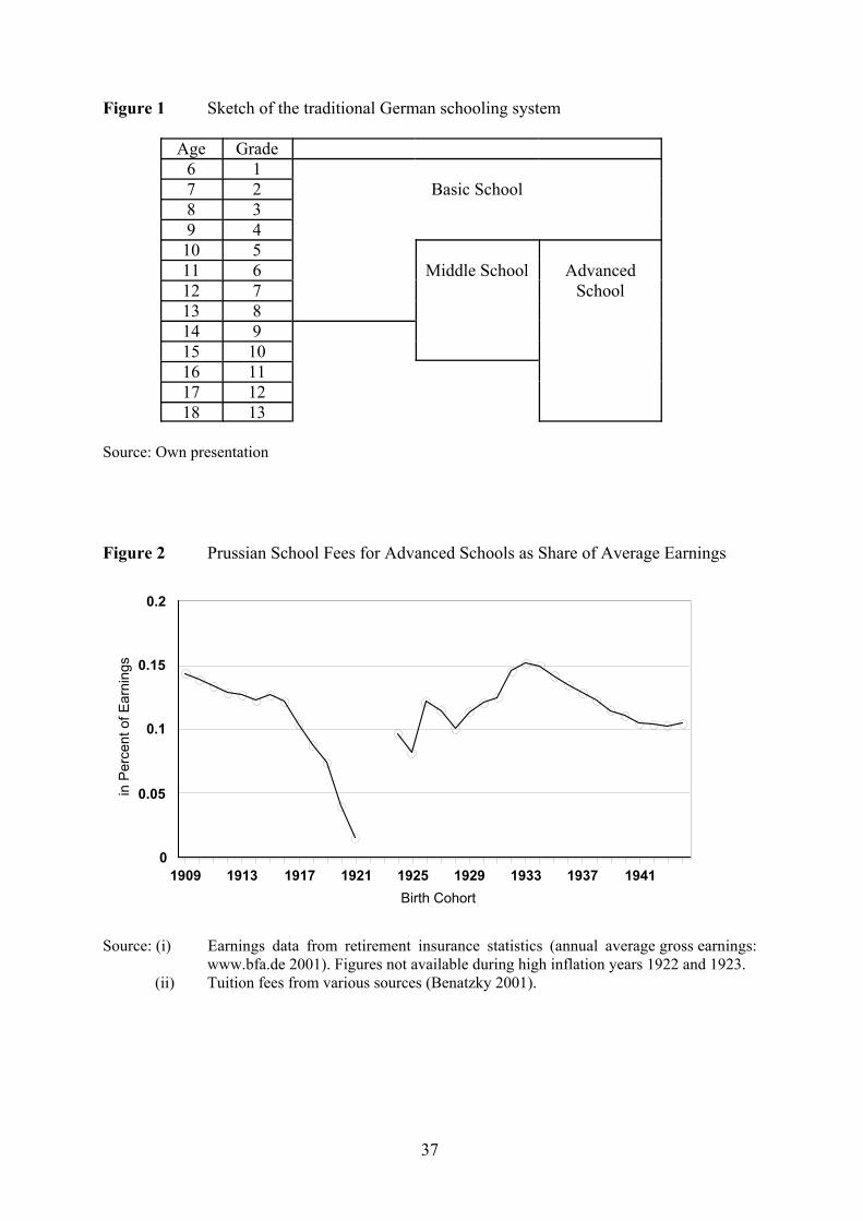
37

Figure 1 Sketch of the traditional German schooling system

Age Grade6 1

Basic School7 28 39 410 511 6 Middle School Advanced

School12 713 814 915 1016 1117 1218 13

Source: Own presentation

Figure 2 Prussian School Fees for Advanced Schools as Share of Average Earnings

1909 1913 1917 1921 1925 1929 1933 1937 1941Birth Cohort

0

0.05

0.1

0.15

0.2

in P

erce

nt o

f Ear

ning

s

Source: (i) Earnings data from retirement insurance statistics (annual average gross earnings:www.bfa.de 2001). Figures not available during high inflation years 1922 and 1923.

(ii) Tuition fees from various sources (Benatzky 2001).

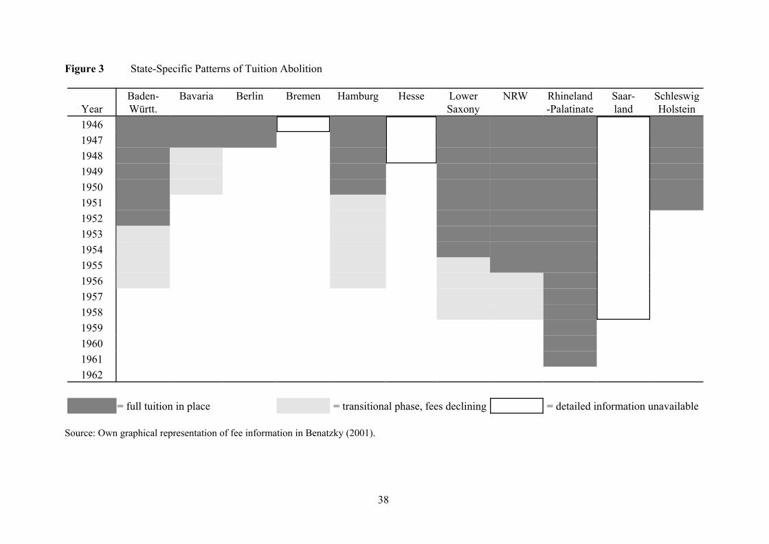
38

Figure 3 State-Specific Patterns of Tuition Abolition

YearBaden-Württ.

Bavaria Berlin Bremen Hamburg Hesse LowerSaxony

NRW Rhineland-Palatinate

Saar-land

SchleswigHolstein

19461947194819491950195119521953195419551956195719581959196019611962

= full tuition in place = transitional phase, fees declining = detailed information unavailable

Source: Own graphical representation of fee information in Benatzky (2001).

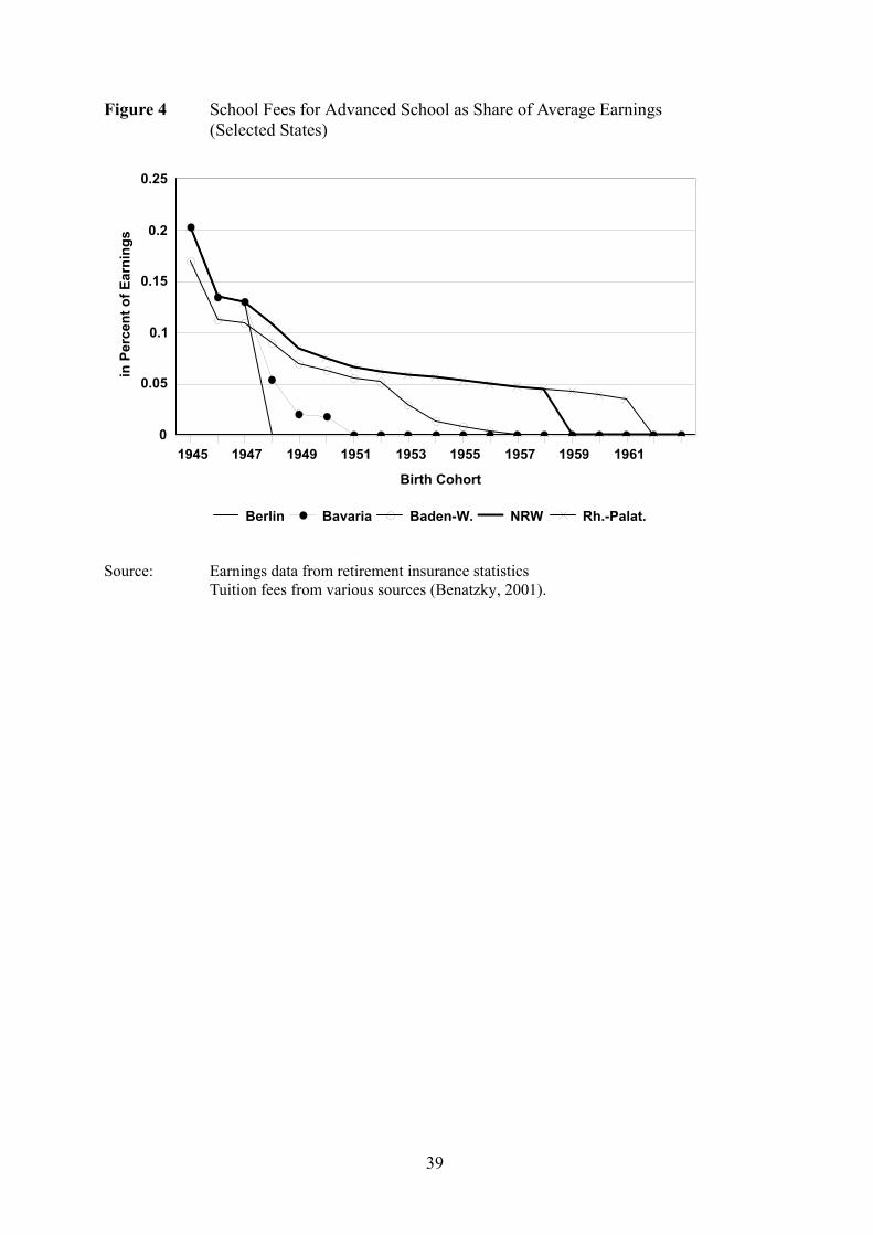
39

Figure 4 School Fees for Advanced School as Share of Average Earnings(Selected States)

1945 1947 1949 1951 1953 1955 1957 1959 1961

Birth Cohort

0

0.05

0.1

0.15

0.2

0.25

in P

erce

nt o

f Ear

ning

s

Berlin Bavaria Baden-W. NRW Rh.-Palat.

Source: Earnings data from retirement insurance statistics Tuition fees from various sources (Benatzky, 2001).

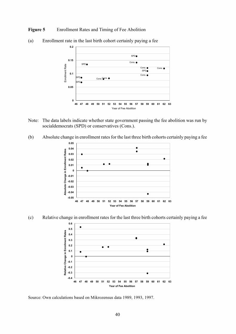
40

Figure 5 Enrollment Rates and Timing of Fee Abolition

(a) Enrollment rate in the last birth cohort certainly paying a fee

Cons.

SPD

SPD

SPD

Cons.

SPD

Cons.

Cons.

Cons.

Cons.

SPD

46 47 48 49 50 51 52 53 54 55 56 57 58 59 60 61 62 63Year of Fee Abolition

0

0.05

0.1

0.15

0.2

Enro

llmen

t Rat

e

Note: The data labels indicate whether state government passing the fee abolition was run bysocialdemocrats (SPD) or conservatives (Cons.).

(b) Absolute change in enrollment rates for the last three birth cohorts certainly paying a fee

46 47 48 49 50 51 52 53 54 55 56 57 58 59 60 61 62 63Year of Fee Abolition

-0.05

-0.04

-0.03

-0.02

-0.01

0

0.01

0.02

0.03

0.04

0.05

Abs

olut

e C

hang

e in

Enr

ollm

ent R

ates

(c) Relative change in enrollment rates for the last three birth cohorts certainly paying a fee

46 47 48 49 50 51 52 53 54 55 56 57 58 59 60 61 62 63Year of Fee Abolition

-0.4

-0.3

-0.2

-0.1

0

0.1

0.2

0.3

0.4

0.5

0.6

Rel

ativ

e C

hang

e in

Enr

ollm

ent R

ates

Source: Own calculations based on Mikrozensus data 1989, 1993, 1997.

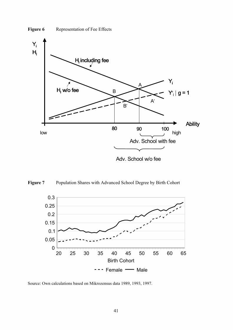
41

Figure 6 Representation of Fee Effects

90 100

Yi

Hi

Hi including fee

Hi w/o fee

Yi

Y‘i * g = 1

80Ability

90 100

Yi

Hi

Hi including fee

Hi w/o fee

Yi

Y‘i * g = 1

80Ability

Yi

Hi

Hi including fee

Hi w/o fee

Yi

Y‘i * g = 1

80Ability

highlow

Adv. School with fee

Adv. School w/o fee

AB

B‘A‘

Figure 7 Population Shares with Advanced School Degree by Birth Cohort

20 25 30 35 40 45 50 55 60 65Birth Cohort

0

0.05

0.1

0.15

0.2

0.25

0.3

Female Male

Source: Own calculations based on Mikrozensus data 1989, 1993, 1997.

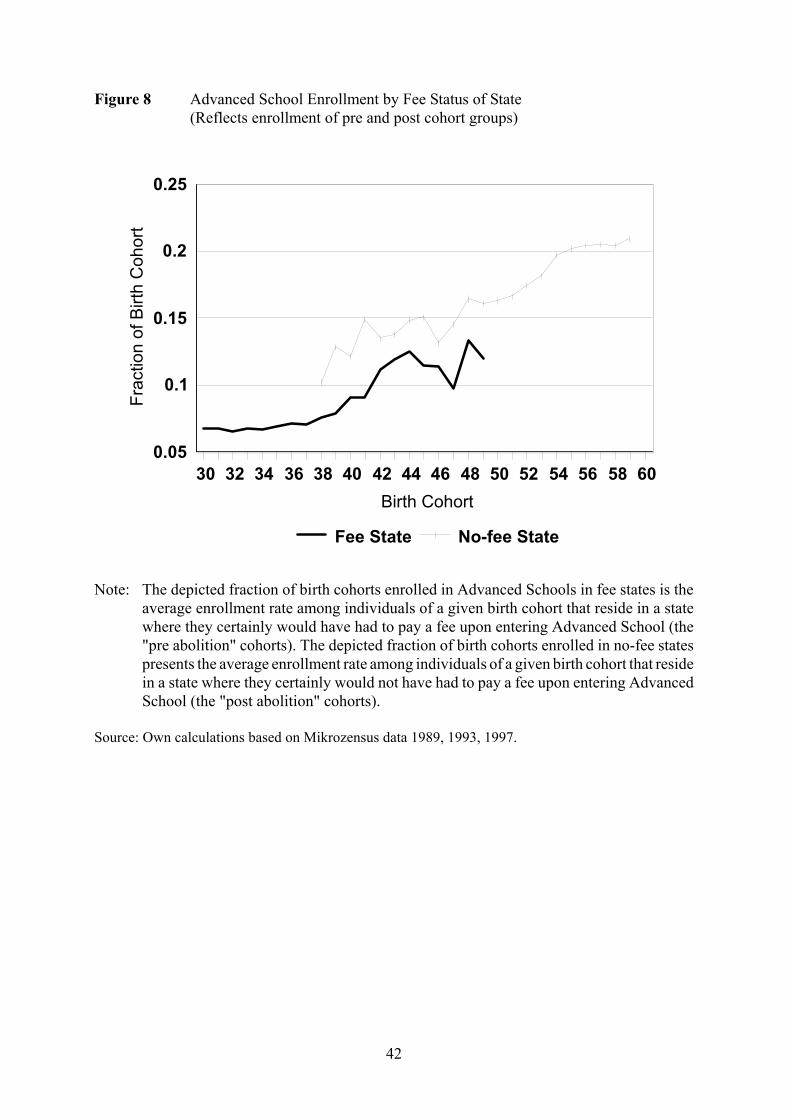
42

Figure 8 Advanced School Enrollment by Fee Status of State (Reflects enrollment of pre and post cohort groups)

30 32 34 36 38 40 42 44 46 48 50 52 54 56 58 60Birth Cohort

0.05

0.1

0.15

0.2

0.25

Frac

tion

of B

irth

Coh

ort

Fee State No-fee State

Note: The depicted fraction of birth cohorts enrolled in Advanced Schools in fee states is theaverage enrollment rate among individuals of a given birth cohort that reside in a statewhere they certainly would have had to pay a fee upon entering Advanced School (the"pre abolition" cohorts). The depicted fraction of birth cohorts enrolled in no-fee statespresents the average enrollment rate among individuals of a given birth cohort that residein a state where they certainly would not have had to pay a fee upon entering AdvancedSchool (the "post abolition" cohorts).

Source: Own calculations based on Mikrozensus data 1989, 1993, 1997.

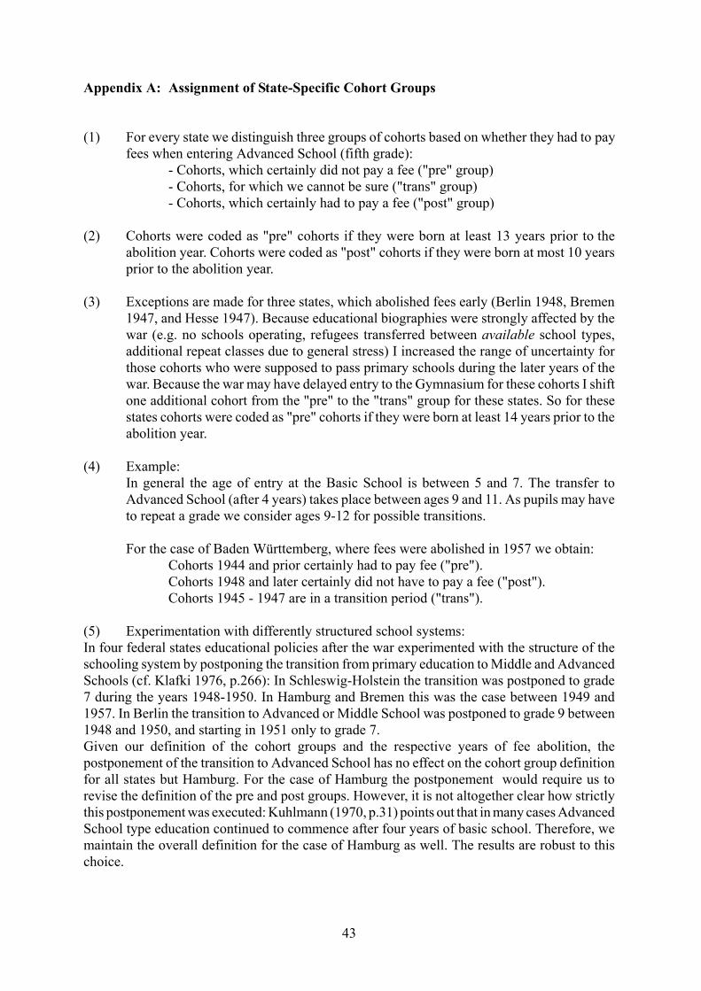
43

Appendix A: Assignment of State-Specific Cohort Groups

(1) For every state we distinguish three groups of cohorts based on whether they had to payfees when entering Advanced School (fifth grade):

- Cohorts, which certainly did not pay a fee ("pre" group)- Cohorts, for which we cannot be sure ("trans" group)- Cohorts, which certainly had to pay a fee ("post" group)

(2) Cohorts were coded as "pre" cohorts if they were born at least 13 years prior to theabolition year. Cohorts were coded as "post" cohorts if they were born at most 10 yearsprior to the abolition year.

(3) Exceptions are made for three states, which abolished fees early (Berlin 1948, Bremen1947, and Hesse 1947). Because educational biographies were strongly affected by thewar (e.g. no schools operating, refugees transferred between available school types,additional repeat classes due to general stress) I increased the range of uncertainty forthose cohorts who were supposed to pass primary schools during the later years of thewar. Because the war may have delayed entry to the Gymnasium for these cohorts I shiftone additional cohort from the "pre" to the "trans" group for these states. So for thesestates cohorts were coded as "pre" cohorts if they were born at least 14 years prior to theabolition year.

(4) Example:In general the age of entry at the Basic School is between 5 and 7. The transfer toAdvanced School (after 4 years) takes place between ages 9 and 11. As pupils may haveto repeat a grade we consider ages 9-12 for possible transitions.

For the case of Baden Württemberg, where fees were abolished in 1957 we obtain: Cohorts 1944 and prior certainly had to pay fee ("pre").

Cohorts 1948 and later certainly did not have to pay a fee ("post").Cohorts 1945 - 1947 are in a transition period ("trans").

(5) Experimentation with differently structured school systems: In four federal states educational policies after the war experimented with the structure of theschooling system by postponing the transition from primary education to Middle and AdvancedSchools (cf. Klafki 1976, p.266): In Schleswig-Holstein the transition was postponed to grade7 during the years 1948-1950. In Hamburg and Bremen this was the case between 1949 and1957. In Berlin the transition to Advanced or Middle School was postponed to grade 9 between1948 and 1950, and starting in 1951 only to grade 7. Given our definition of the cohort groups and the respective years of fee abolition, thepostponement of the transition to Advanced School has no effect on the cohort group definitionfor all states but Hamburg. For the case of Hamburg the postponement would require us torevise the definition of the pre and post groups. However, it is not altogether clear how strictlythis postponement was executed: Kuhlmann (1970, p.31) points out that in many cases AdvancedSchool type education continued to commence after four years of basic school. Therefore, wemaintain the overall definition for the case of Hamburg as well. The results are robust to thischoice.

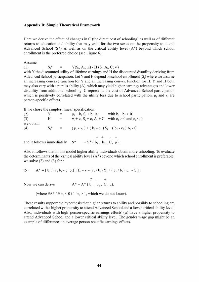
44

Appendix B: Simple Theoretical Framework

Here we derive the effect of changes in C (the direct cost of schooling) as well as of differentreturns to education and ability that may exist for the two sexes on the propensity to attendAdvanced School (S*) as well as on the critical ability level (A*) beyond which schoolenrollment is the preferred choice (see Figure 6).

Assume(1) Si* = Y(Si, Ai; :i) - H (Si, Ai, C; <i) with Y the discounted utility of lifetime earnings and H the discounted disutility deriving fromAdvanced School participation. Let Y and H depend on school enrollment (Si) where we assumean increasing concave function for Y and an increasing convex function for H. Y and H bothmay also vary with a pupil's ability (A), which may yield higher earnings advantages and lowerdisutility from additional schooling. C represents the cost of Advanced School participationwhich is positively correlated with the utility loss due to school participation. :i and <i areperson-specific effects.

If we chose the simplest linear specification:(2) Yi = :i + b1 Si + b2 Ai with b1 , b2 > 0(3) Hi = <i + c1 Si + c2 Ai + C with c1 > 0 and c2 < 0we obtain(4) Si* = ( :i - <i ) + ( b1 - c1 ) Si + ( b2 - c2 ) Ai - C

+ + - +and it follows immediately S* = S* ( b1 , b2 , C, :).

Also it follows that in this model higher ability individuals obtain more schooling. To evaluatethe determinants of the 'critical ability level' (A*) beyond which school enrollment is preferable,we solve (2) and (3) for :

(5) A* = [ b1 / (c2 b1 - c1 b2)] [Hi - <i - (c1 / b1) Yi + ( c1 / b1) :i - C ] .

? - + -Now we can derive A* = A* ( b1 , b2 , C, :).

(where MA* / M b1 < 0 if b1 > 1, which we do not know).

These results support the hypothesis that higher returns to ability and possibly to schooling arecorrelated with a higher propensity to attend Advanced School and a lower critical ability level.Also, individuals with high 'person-specific earnings effects' (:) have a higher propensity toattend Advanced School and a lower critical ability level. The gender wage gap might be anexample of differences in average person-specific earnings effects.