Working Paper/Document de travail 2015-30

The Endogenous Relative Price of Investment

by Joel Wagner

2

Bank of Canada Working Paper 2015-30

July 2015

The Endogenous Relative Price of Investment

by

Joel Wagner

Canadian Economic Analysis Department Bank of Canada

Ottawa, Ontario, Canada K1A 0G9 jwagner@bankofcanada.ca

Bank of Canada working papers are theoretical or empirical works-in-progress on subjects in economics and finance. The views expressed in this paper are those of the author.

No responsibility for them should be attributed to the Bank of Canada.

ISSN 1701-9397 © 2015 Bank of Canada

ii

Acknowledgements

I would like to first thank my supervisor Marc-André Letendre from McMaster University for his insights. His efforts to improve upon the strengths of this paper are highly appreciated. I would like to also thank Alok Johri and William Scarth for their contributions to the crafting of this paper. Lastly, I would like to thank those who attended the 2015 Toronto CEA conference presentation of this paper for their suggestions and comments.

iii

Abstract

This paper takes a full-information model-based approach to evaluate the link between investment-specific technology and the inverse of the relative price of investment. The two-sector model presented includes monopolistic competition where firms can vary the markup charged on their product depending on the number of firms competing. With these changes to the standard two-sector model, both total factor productivity as well as a series of non-technological shocks can impact the high-frequency volatility of the relative price of investment. Utilizing a Bayesian estimation approach to match the model to the data, we find that investment-specific technology can explain at most half of the growth rate of the relative price of investment. Last of all, we compare the benchmark model results with endogenous movement in the relative price of investment to a model where all movement in the relative price of investment is derived exogenously. This is done by allowing technologies across sectors to move together over time. Comparison of these two methods finds that the exogenous approach is incapable of capturing changes in the relative price of investment as found in the data. This paper adds to the growing list of research, like that of Fisher (2009) and Basu et al. (2013), that suggests that the quality-adjusted relative price of investment may be a poor indicator of investment-specific technology.

JEL classification: E32, L11, L16 Bank classification: Business fluctuations and cycles

Résumé

L’auteur utilise une méthode d’analyse basée sur un modèle structurel et des données complètes pour évaluer le lien entre les chocs technologiques spécifiques à l’investissement et l’inverse du prix relatif de l’investissement. Il propose un modèle bisectoriel intégrant une structure de concurrence monopolistique où les entreprises peuvent faire varier le taux de marge appliqué à leur produit en fonction du nombre de firmes concurrentes. Compte tenu de cette adaptation du modèle bisectoriel standard, aussi bien la productivité totale des facteurs qu’une série de chocs non technologiques peuvent avoir une incidence sur la volatilité à haute fréquence du prix relatif de l’investissement. L’auteur emploie une méthode d’estimation bayésienne pour faire concorder le modèle et les données, et il constate que les chocs technologiques spécifiques à l’investissement peuvent expliquer tout au plus la moitié du taux de croissance du prix relatif de l’investissement. Enfin, il compare les résultats obtenus à l’aide du modèle de référence dans lequel les variations du prix relatif de l’investissement sont endogènes aux résultats d’un modèle où tout mouvement du prix relatif de l’investissement est déterminé de façon exogène. À cette fin, les technologies suivent une évolution parallèle au fil du temps tous secteurs confondus. La comparaison de ces deux méthodes permet de constater que l’approche exogène ne peut pas rendre compte des changements du prix relatif de l’investissement qui ressortent des données.

iv

Cette étude enrichit le corpus de recherches qui, comme celles de Fisher (2009) et de Basu et coll. (2013), laissent entrevoir que le prix relatif de l’investissement corrigé des variations de qualité est peut-être un mauvais indicateur des chocs technologiques spécifiques à l’investissement.

Classification JEL : E32, L11, L16 Classification de la Banque : Cycles et fluctuations économiques

Non-Technical Summary

Motivation and QuestionWhat drives the business cycle? In the literature, two types of technology shocks have beenidentified as potential sources of business cycle volatility. These include neutral technol-ogy shocks (which improve productivity economy-wide) and investment-specific technologyshocks (such as innovations in communication technology). Traditionally, investment-specifictechnology (IST) has been identified by the inverse of the relative price of investment (RPI).This identification scheme assumes, however, that the RPI is not influenced by shifts in in-vestment demand. This paper explores the validity of this assumption. That is, does the RPIvary with investment demand? Given their relevance in explaining business cycle volatility,this subject warrants investigation.

MethodologyThis paper proposes a two-sector model adapted to allow for monopolistic competition in theproduction of both consumption and investment sector intermediate goods. It is assumedthat the number of firms operating within each sector is finite, thus allowing firms to varytheir markup depending on the number of existing competitors. The model is then perturbedby both stationary and non-stationary neutral and investment-specific technology shocks aswell as three non-technological shocks. This model is compared to an alternative modelwhere business cycle movement in the RPI is modeled exogenously by allowing both neutraland investment-specific technology to follow a common stochastic trend. Bayesian estimationis used for the model’s parameterization, followed by a decomposition to assess each shock’scontribution to the volatility of the RPI. These two models are then assessed by the ability ofneutral technology as well as shifts in investment demand (relative to consumption demand)to generate volatility in the growth rate of the RPI.

Key ContributionsThis paper finds that over half of the volatility of the RPI can be attributed to shifts ininvestment demand, with the remainder due to shifts in IST. This result is in sharp con-trast to the longstanding assumption in the macroeconomic literature that movement in theRPI is purely a technological phenomenon. This paper adds to the current business cycleliterature by demonstrating that IST shocks are not only incapable of generating realisticbusiness cycles (as is the current assumption in the literature), but are incapable of gener-ating volatility in the RPI itself. These results suggest that calibrating IST shocks to theinverse of the RPI overestimates the relative importance of IST. This paper also validatesthe current assumption in the literature that changes in the marginal efficiency of investment(such as changes in the firm’s ability to access credit) do not impact the RPI.

Future ResearchThis paper addresses the co-movement of total factor productivity and IST endogenously overthe short run. It is, however, incapable of reproducing the common trend component betweenthese two technologies observed in the data in the long run. Given the potential relevanceof both neutral and investment-specific technology in generating growth in the Canadianeconomy, future research should be done to uncover the source of this relationship.

1 Introduction

Since Greenwood, Hercowitz, and Huffman (GHH) (1988) first identified investment-specifictechnology (IST) as a potential source of business cycle volatility, this type of shock hasbecome a common feature in the business cycle literature. Likewise, identification of ISThas remained roughly in line with the method used by Greenwood, Hercowitz, and Krusell(GHK) (1997), who built upon the work done by GHH (1988). Since their seminal work, thebusiness cycle literature has shifted over time in its assessment of the relative importanceof IST. At first, research such as that by Fisher (2006) as well as Justiniano, Primiceri,and Tambalotti (2010) found IST to be an important source of both low-frequency andhigh-frequency volatility. Each time, the relative importance of IST is assessed by eitheranalyzing the variance decomposition or by growth accounting (as done by Fisher (2006)).Recent research, such as that of Justiniano et al. (2011) and Schmitt-Grohe and Uribe(2011), has, however, found that IST, when correctly adapted to reflect movement in therelative price of investment (RPI), lacks the ability to generate any business cycle volatility.

Beaudry and Lucke (2009) take an alternative approach. In their research, rather thananalyzing a dynamic stochastic general-equilibrium model’s variance decomposition, theyquantitatively assess the relative importance of IST against a menu of alternative shocksusing an approach based on a cointegrated structural vector autoregression (SVAR). Theyconclude that expected changes in neutral technology, as well as preference and monetaryshocks, play a far more significant role in explaining high-frequency movements in the datain their forecast-error variance decomposition than IST. All of the aforementioned researchrelies heavily on the assumption that IST can be uniquely identified by the inverse of theRPI. Using micro-level data, Basu et al. (2013) show that the RPI responds slowly to changesin IST, often taking up to three quarters for the effect of an IST shock to impact the RPI.This could be due to either sticky investment prices, or, alternatively, investment prices thatare driven by forces other than IST. Through an SVAR-based approach, Kim (2009) findsthat IST shocks could at most explain 27 percent of the RPI from 1955Q1 to 2000Q4. Theassumption that IST is an independent stochastic process implies that the RPI is orthogonalto any other type of economic disturbance, such as neutral technology shocks, wage shocks orpreference shocks, which are commonly included in the literature. Therefore, the adequacyof the RPI to correctly indicate movements in IST could, for example, be assessed by theindependence of the RPI from any one of these disturbances. If the inverse of the RPI, asGHK (1997) suggested, is a good indication of IST, then these technology shocks should intheory be unrelated to neutral technology as measured by total factor productivity (TFP).

As can be seen in Figure 1, upturns in log TFP (tfp) are typically followed by a decreasein the log RPI (rpi). The tfp plotted in Figure 1 is calculated as in Beaudry and Lucke(2009) (the log of non-farm output less the log of both non-farm hours and capital services,each scaled by its share of output).1 As for the rpi, we use the quality-adjusted rpi time

1Data on the real non-farm gross value-added output are calculated by the Bureau of Economic Analysis1947Q1 to 2013Q4. Non-farm hours worked are calculated by the Bureau of Labor Statistics (BLS) 1947Q1to 2013Q4. Capital services time series are calculated from the (BLS) private sector non-farm business sector

2

series as calculated by Fisher (2006). This data series adjusts the relative price of equipmentestimated by using the Gordon-Cummins-Violante equipment price deflator and divides itby the quarterly price deflator for consumption goods found in the U.S. national incomeand product accounts (NIPA) tables. With these two time series, Fisher (2006) obtains aquarterly measure of the rpi adjusted for changes in quality. Information on the data usedis available in the appendix.

With a correlation between detrended tfp and rpi of approximately -0.216, it wouldappear that the rpi moves countercyclically to tfp. This fact has been addressed in countlesspapers, such as that of Letendre and Luo (2007), who adapt the standard AR(1) set-up toallow for spillovers between tfp and rpi in order to replicate the countercyclical nature ofthe rpi. Thus, it appears that in the short run, the theory suggested by GHK (1997) thatrelative prices can be used to determine changes in relative technologies across sectors is lessthan robust.

Schmitt-Grohe and Uribe (2011) have furthered the disconnect between IST and the rpiby also demonstrating that tfp and the rpi are cointegrated in the long run. With both tfp andthe rpi integrated of order 1 stationary in the United States, they apply a Johansen’s test forcointegration in which they show that in addition to tfp and rpi being non-stationary, theyare also cointegrated.2 With both tfp and the rpi cointegrated, there exists a cointegrationcoefficient β such that the difference in levels between each time series remains I(0) stationaryin the long run. To highlight this fact, Figure 2 plots tfp along with the inverse of the rpiadjusted by the cointegration coefficient β = 0.623. Figure 2 demonstrates that these twotime series follow a common stochastic trend. Given the assumption made by GHK (1997)that relative technologies across sectors are reflected in the relative price, it would be expectedthat these two time series would not follow a common stochastic trend, as both cointegrationtests, as well as Figure 2, appear to suggest. As is shown in section 4, when the standardbusiness cycle model is adapted to replicate the co-movement of tfp and the rpi, 31 percentof rpi growth from one period to the next can be explained by shifts in neutral technology.

Given the aforementioned relationships between tfp and the rpi, both in the long run andover the business cycle, the assumption that the rpi is orthogonal to any form of economicdisturbance can be safely rejected. Further tests could be done to assess the orthogonalityof the rpi with any other form of economic disturbances, such as wage markup, preferenceshocks or shifts in the marginal efficiency of investment.

Is the cyclical movement in the rpi a technological phenomenon, or is movement in therpi due to changes in the relative demand for investment goods over consumption goods?In response to this question, this paper proposes a two-sector model adapted to incorporateendogenous markup variation within each sector. Endogenous price markups are incorpo-

(NAICS 113-81) 2009 index 1987-2012.2Schmitt-Grohe and Uribe (2011) apply both an Augmented Dickey Fuller Test (ADF) as well as a

Kwiatkowski, Phillips, Schmidt, and Shin (KPSS) test to determine the stationarity of both tfp and the rpi.As can be seen in Tables 1 and 2 of Schmitt-Grohe and Uribe (2011), both of these tests conclude that thesetwo series are non-stationary.

3

rated by assuming that each sector (consumption and investment) is populated by a finitenumber of firms, each selling a differentiable good. Each of these firms is capable of notonly influencing its own price, but also the price charged across all firms. An alternativemodel is presented in section 4, where movement in the rpi is generated entirely by techno-logical spillovers. As section 4 demonstrates, when the assumption of orthogonality betweentechnologies is relaxed, approximately 31 percent of the rpi can be attributed to shifts intfp. In contrast, when the rpi moves in response to changes in demand, as is the case in thebenchmark model, the explanatory power of IST drops further to 45 percent. Stationary andnon-stationary tfp shocks explain approximately 29 percent of the volatility of the rpi. Non-technological shocks contribute 26 percent. With the vast majority of business cycle researchassuming that the rpi is determined exogenously, the results of this paper are particularlypoignant.

These two approaches are compared to Kim’s (2009) research to assess whether one ap-proach outperforms the other. As outlined in section 4, our results indicate that an endoge-nous approach to modeling movement in the rpi outperforms the exogenous-based approach,due to the impact non-technological shocks have on the relative demand for investment goodsover consumption goods. Through the endogenous-based approach, 45 percent of the volatil-ity of the rpi is explained by unanticipated changes in IST. These results bring into questionthe current convention in linking IST to the inverse of the rpi.

The remainder of the paper is organized as follows. Section 2 outlines the benchmarkmodel, consisting of the varying elements that allow the rpi to move endogenously over time.Section 3 outlines the Bayesian estimation process, which is used to estimate the parametervalues. Section 4 outlines the results of the benchmark model with variations of this model, toassess the relative importance of each aspect in generating these results. Section 5 concludes.

2 Benchmark Model

The benchmark model for this paper involves a two-sector real business cycle model withmonopolistic competition in both consumption- and investment-goods-producing sectors.This model is set up in such a way that firms are able to vary the markup charged aboveproduction costs depending on the number of competing firms within that industry. Webegin with an outline of the various stages of production in the consumption sector.

Production of each good can be divided into three stages of production. These stagesinclude a finite number of monopolistically competitive firms that produce their productusing both capital and labour inputs. These goods are then aggregated at an industry levelby firms that assemble them into a composite good to be sold at the sector level. Lastly,there is a perfectly competitive firm that purchases these industry-level goods and assemblesthem into a composite good ready to sell to consumers. For ease of illustration, we beginour dissection of the various stages of consumption production at the sector level.

4

2.1 Consumption Sector

2.1.1 Sector Level

At the aggregate level, the consumption good produced in this economy Ct is a compositegood consisting of a continuum of unit measure one industry-level goods produced using thefollowing constant-returns-to-scale production function:

Ct =

[ ∫ 1

0

Qct(j)

ωdj

] 1ω

, (1)

where Qct(j) refers to the quantity of output produced in industry j, with the elasticity of

substitution between industry-level goods equal to 11−ω . The total profit earned by assembling

these industry-level goods at the sector-level Πct is equal to

Πct =

{P ct Ct −

∫ 1

0

P ct (j)Qc

t(j)dj

}, (2)

where PCt is the price of the sector-level consumption good and P c

t (j) is the price paid for in-dustry j’s composite good. Solving the production problem for the sector-level consumption-goods producer implies a conditional input demand of

Qct(j) =

(P ct (j)

P ct

) 1ω−1

Ct (3)

of industry j’s good by the sector-level producer, where the price index P ct is equal to

P ct =

[ ∫ 1

0

PCt (j)

ωω−1 dj

]ω−1ω

. (4)

2.1.2 Industry Level

The industry-level consumption good is produced using a constant-returns-to-scale produc-tion function which aggregates output produced by a finite number of firms within industryj. Firm i within industry j produces a differentiable good xct(j, i). This good is used as aninput at the industry level through the following production function:

5

Qct(j) =

[N ct (j)

]1− 1τ

[ Nct∑

i=1

xct(j, i)τ

] 1τ

. (5)

N ct (j) denotes the number of firms competing in industry j and 1/(1 − τ) is the elasticity

of substitution between industry-level goods. Given this production function, the profitfunction for the firm producing the industry j good Πc

t(j) is determined as

Πct(j) =

P ct (j)Qc

t(j)−Nct (j)∑i=1

xct(j, i)pct(j, i)

, (6)

where PCt (j, i) denotes the price of firm i’s output in industry j. This profit function implies

a conditional demand

xct(j, i) =(P c

t (j, i)

P ct (j)

) 1τ−1 Qc

t(j)

N ct

(7)

by industry j for firm i’s product. Analogous to the sector level of production, the industryj consumption-good price index is equal to

P ct (j) = N c

t (j)1τ−1

[Nct (j)∑i=1

P ct (j, i)

ττ−1

] τ−1τ

. (8)

2.1.3 Firm Level

The last stage of production consists of a finite number of monopolistically competitive firmswithin each industry. These firms produce a good using both capital and labour as inputs.We assume that these firms can costlessly differentiate their product, and thus, given a finitenumber of firms competing, have the ability to not only influence its own price P c

t (j, i), butalso the industry-level price P c

t (j). While firm i in industry j has the ability to influenceP ct (j, i) as well as P c

t (j), it does not have the ability to influence the sector-level price P ct . In

industry j, firm i’s good is produced using the following constant-returns-to-scale productionfunction:

xct(j, i) = Zt(kct (j, i)

)α(Xzt h

ct(j, i)

)1−α − φc where φc > 0, 0 < α < 1, (9)

where kct (j, i) and hct(j, i) denote the capital and labour used by firm i in industry j, respec-

6

tively, α is the capital share of output, and φc denotes the fixed cost of production. We assumethat there are two types of technology shocks affecting production of consumption goods.These include a stationary technology shock, Zt, and a non-stationary labour-augmentingtechnology, Xz

t , where the stochastic growth rate of XZt is given by

µzt ≡Xzt

Xzt−1

. (10)

TFP in the consumption sector is

TFPt = Zt(Xzt

)1−α. (11)

Given the conditional input demand for industry-level consumption goods by the sector-level firm (equation (3)) and industry j’s conditional input demand by industry j for firm i’sconsumption good (equation (7)), we can write the conditional demand for firm i’s good as

xct(j, i) =

[P ct (j, i)

P ct (j)

] 1τ−1[P ct (j)

P ct

] 1ω−1 Ct

N ct (j)

. (12)

Thus, firm i maximizes profits by choosing its capital and labour demand as well as a priceP ct (j, i) that maximizes profit:

Πct(j, i) = {P c

t (j, i)xct(j, i)− wcthct(j, i)− rctkct (j, i)} , (13)

subject to its production function (9).

Solving the firm-level problem, we get

P ct (j, i) = µct(N

ct (j))MCc

t (j, i) =(1− ω)N c

t (j)− (τ − ω)

τ(1− ω)N ct (j)− (τ − ω)

MCct (j, i), (14)

where MCct (j, i) is the marginal cost of production by firm i in sector j and µct(N

ct (j)) is the

markup charged by this firm. The firm’s optimal labour demand implies a wage rate in theconsumption sector,

wct =P ct (j, i)

µct(j, i)αZc

t

(kct (j, i)

hct(j, i)

)αXzt

1−α, (15)

7

and a rental rate

rct =P ct (j, i)

µct(j, i)(1− α)Zc

t

(kct (j, i)

hct(j, i)

)α−1

Xzt

1−α. (16)

The markup charged over production costs by this firm is determined by both the numberof firms competing in their industry and the substitutability of its goods within and acrossindustries.

It is assumed that firm-level technology is identical both within and across industriesin the consumption sector. This assumption implies that for every firm i ∈ [0, N c

t (j)] andfor every industry j ∈ [0, 1], firms make identical decisions when choosing both labourand capital services (hct(j, i) = hct , k

ct (j, i) = kct ). This implies that the quantity of goods

produced by each firm will also be the same across all firms (xct(j, i) = xct) . Furthermore,with this assumption we can generalize the price charged by firms along with the price indexat both an industrial level (equation (8)) and at a sector level (equation (4)), implying thatP ct (j, i) = P c

t (j) = P ct .

As mentioned earlier, the firm incurs a fixed cost of production φct , which we set accordingto the following zero-profit condition:

φct = xct(µct − 1), (17)

along a balanced growth path (BGP). Given N ct firms in each industry, we can calculate the

quantity of consumption goods produced Ct as

Ct = Qct = N c

t xct =

Ztµct

(kct )α(Xz

t hct)

1−α. (18)

With this equation along with the zero-profit condition outlined in equation (17), we cancalculate the total number of firms operating within each industry as

N ct =

µct − 1

µctφcZct (k

ct )α(XZ

t hct)

1−α. (19)

2.2 Investment Sector

Thus far we have outlined the various stages of production in the consumption-goods sector.The investment sector shares a similar structure to the consumption-goods sector, havinga finite number of monopolistically competitive firms selling their differentiable products toa continuum of unit measure one industry-level firms, who in turn sell these goods to thesector-level producer. Similar to the consumption sector, we begin our description of theinvestment-goods sector at the sectoral level.

8

2.2.1 Sector Level

Sector-level investment goods are produced by amalgamating a continuum of industry-levelinvestment goods according to the following constant-returns-to-scale production function:

It =

[ ∫ 1

0

QIt (j)

ωdj

] 1ω

. (20)

As was the case in the consumption sector, the final good produced in the investmentsector It is a composite good consisting of a continuum of industry-level investment goodsQIt (j) of unit measure one. The profit function for the investment-good producer at the

sector level is

ΠIt =

{P It It −

∫ 1

0

P It (j)QI

t (j)dj

}, (21)

where P It (j) is the price of industry j’s investment good and QI

t (j) denotes the quantityof investment goods produced in industry j. As was the case in the consumption sector,industry-level investment goods are not perfect substitutes but rather have an elasticity ofsubstitution determined by 1/(1− ω).

2.2.2 Industry Level

At the industry level, the investment-goods sector is symmetric in construction to theconsumption-goods sector at the same level of production. The industry-level compositegood is produced using the following constant-returns-to-scale production function:

QIt (j) =

(N It (j)

)1− 1τ

[NIt (j)∑i=1

xIt (j, i)τ] 1τ

. (22)

The conditional input demand for the firm-level good xIt (j, i) by industry j is then calculatedas

xIt (j, i) =

(P It (j, i)

P It (j)

) 1τ−1 QI

t (j)

N It

, (23)

with the price index P It (j) in industry j equal to

9

P It (j) = N I

t (j)1τ−1[NI

t (j)∑i=1

P It (j, i)

ττ−1

] τ−1τ

. (24)

2.3 Firm Level

The firm-level investment good, xIt (j, i), is produced using the following production function:

xIt (j, i) = ZtAtkIt (j, i)

α(XZt X

At h

It (j, i)

)1−α − φI , (25)

where kIt (j, i) and hIt (j, i) denote the capital and labour services used by firm i in industry j,φI is the fixed cost of production, and α denotes the capital share of output. As was the casein the consumption-goods sector, technology in the investment sector can be broken downinto two separate components. There is a stationary IST shock At as well as the stationarytfp shock Zt. There is also a non-stationary labour-augmenting technology XA

t (j) specific tothe investment sector, along with the neutral technology XZ

t (j). The non-stationary IST isassumed to follow a stochastic growth rate, defined as

µAt ≡XAt

XAt−1

. (26)

IST is measured as

ISTt = At(XAt

)(1−α). (27)

With each firm i selling a differentiable good in industry j, firms compete on price, thusallowing investment firms to sell their product at a markup µIt above their respective marginalcost MCI

t (j, i):

P It (j, i) = µIt (N

It (j))MCI

t (j, i) =(1− ω)N I

t − (τ − ω)

τ(1− ω)N It − (τ − ω)

MCIt (j, i). (28)

As was the case in the consumption sector, with symmetric technologies across industries,we can drop all indexes. The fixed cost of production is set equal to

φIt = xIt (µI − 1). (29)

This is used to remove firm profits along a BGP. With this information, we can calculate

10

the number of firms in the investment sector as

N It =

(µIt − 1)

µItφIZtAtk

It

α(XZt X

At h

It

)1−α. (30)

This implies a total output in the investment sector of

It =ZtAtµIt

kItα(XZt X

At h

It

)1−α. (31)

The real wage and rental rates in the investment sector are

wIt =P I

µItαZtAtk

It

αhIt−αXZt X

At

(1−α)(32)

rIt =P I

µIt(α− 1)ZtAtk

It

α−1(XZ

t XAt h

It )

(1−α). (33)

With both labour and capital perfectly mobile between sectors, we have

wIt = wCt and rIt = rCt . (34)

Dividing the wage rate in the investment sector by the wage rate in the consumptionsector, we can estimate the rpi as

P It

P ct

=µItµCt

1

At

(kCthCt

)α(kIthIt

)−αXAt

(α−1). (35)

2.4 Households

The economy consists of a large number of identical and infinitely lived households who,by choosing consumption Ct and hours worked Ht, maximize their expected lifetime utilitysubject to their budget constraint, with a lifetime utility of

E0

∞∑t=0

βtU(Ct, Ht), (36)

11

where 0 < β < 1 is the subjective discount factor. The households’ periodic utility functionis represented using Jaimovich and Rebelo preferences:

U(Ct, Ht) =bt(Ct − χCt−1 − ΓHΘ

t Xt)1−σ − 1

1− σ(37)

Xt = (Ct − χCt−1)ηX1−ηt−1 , (38)

where Γ > 0, Θ > 1, σ > 0, χ > 0, and 0 < η < 1. Here Θ determines the level oflabour supply elasticity and σ determines the curvature of household utility, χ is the habitpersistence parameter, and η determines the effect wealth has on household labour supplydecisions. The elements included in the periodic utility function that are distinctive to thestyle of preferences used by Jaimovich and Rebelo (2009) are the preference parameter ηand the latent variable Xt. These preferences have become popular due to their ability todial up or dial down the wealth effect on labour supply. When η is close to 1, we haveKing, Plosser, and Rebelo (1988) preferences (strong wealth effect). When η is closer to0, we have GHH (1988) preferences, with a limited wealth effect on labour supply. Last ofall, preference shocks bt, which alter the households’ intertemporal consumption and laboursupply decisions are included in the benchmark model.

Households can accumulate capital according to the following capital accumulation equa-tion:

Kt+1 = (1− δ)Kt + vtIt, (39)

where Kt is the households’ capital stock and It is the real quantity of investment goodspurchased in period t. We also include a marginal efficiency of investment (MEI) vt. Theseshocks have become popular in the literature since Justiniano et al. (2011) demonstrated thatthey are an important determinant of volatility in investment growth over the business cycle.The households’ labour and capital services are used by both capital- and consumption-goods-producing firms. The household budget constraint is given by the following formula:

PCt Ct + P I

t It =wtHt

µw+ rtK

Ht + ΠC

t + ΠIt + Ψt. (40)

Given that wages earned in each sector are equal (labour supply is perfectly mobile), thehousehold earns a labour income of wtHt/µ

w for hours worked in each sector, where Ht

denotes the number of hours supplied by households in period t, wt denotes the wages paid,and wt/µ

w denotes the wages earned by the household adjusted by a wage markup shock.Here I assume that the portion of wages taken from the household through the wage markupshock are rebated back to the household via a lump sum transfer Ψt. Households alsoearn a rental income from capital services provided to both sectors rtKt. Since households

12

own both consumption- and investment-goods-producing firms, any profits ΠCt and ΠI

t areaccrued to the household. Given the prices PC

t and P It for consumption and investment

goods, respectively, households purchase Ct consumption goods and It investment goods, allmeasured in real terms.

With households as the only source of labour in this model, the market-clearing conditionsin the labour markets imply that labour supply Ht equals the sum of labour demand in bothsectors. With NC

t firms operating within the consumption sector and N It firms within the

investment sector, this equilibrium condition implies that

Ht = NCt h

Ct +N IhIt . (41)

Normalizing the population of entrepreneurs to 1, the capital market clears when

Kt = NCt k

Ct +N I

t kIt . (42)

Last of all, with all firms within each sector identical, the total amount of consumption andinvestment goods produced is calculated as follows:

Ct = NCt x

Ct , (43)

and

It = N It x

It . (44)

2.5 Exogenous Shocks

Altogether, we have seven types of shocks. There are technology shocks, which include bothstationary and non-stationary tfp as well as stationary and non-stationary IST shocks. Thenon-technology shocks include wage markup, preference and MEI, each of which is assumedto be stationary. For stationary shocks Zt and At, we assume the following AR(1) processes:

ln(Zt) = ρZ ln(Zt−1) + εZt (45)

ln(At) = ρAln(At−1) + εAt , (46)

13

where 0 < ρZ < 1, 0 < ρA < 1 refers to the level of persistence for each shock, while eZt andεAt are unanticipated shocks to ln(Zt), and ln(At), respectively. The steady-state values ofZt and At are normalized to one. Innovations εZt and εAt , have an expected value of zero,with variance σZt and σAt respectively. As for the non-stationary components for neutraland investment-specific technology, we assume that each technology experiences stochasticgrowth rates according to the following laws of motion:

ln(µZt /µZ) = ρµZ ln(µZt−1/µ

Z) + σµZ

εµZ

t (47)

ln(µAt /µZ) = ρµAln(µAt−1/µ

A) + σµA

εµA

t , (48)

where the growth rates in TFP and IST are calculated as in equations (10) and (26), re-spectively. The persistence of each disturbance ρzµ and ρAµ is assumed to be between 0 and

1. The innovations in tfp growth εµz

t and IST growth εµA

t are unanticipated, with a standard

deviation σµZ

t and σµA

t , respectively. Lastly, µZ and µA denote the steady-state values of µZtand µAt , which are discussed in the next section.

There are three stationary non-technological shocks – wage markup, preference and MEIshocks – which move according to the following laws of motion, respectively:

ln(µw

µw) = ρµw ln(

µwt−1

µw) + σµ

w

εµw

t (49)

ln(bt) = ρbln(bt−1) + σbεbt (50)

ln(vt) = ρvln(vt−1) + σvεvt . (51)

Each of the persistence parameters ρµw , ρb and ρv is between 0 and 1. Each innovationlisted above is assumed to be i.i.d. with mean 0 and variance of 1 and with a standarddeviation of σµw , σb and σv, respectively.

With both non-stationary neutral and investment-specific technology, each variable dis-cussed thus far must be detrended wherever a trend is present. With the trend in neutraltechnology denoted by XZ

t , the trend in output XYt has the following form:

XY = XZt

(XAt

)α, (52)

where consumption, nominal investment, output and the fixed cost of production in theconsumption sector all share this same trend. As for the trend of the capital stock Xk

t , the

14

trend in the fixed cost of investment production and the trend of real investment XIt , we

have

XI = XZt X

At . (53)

We normalize the price of consumption goods PCt to 1. The trend in the rpi is equal to

XP I

t =(XAt

)α−1). (54)

There is no growth in hours, price markups or the number of firms within an industry.Letting µY ≡ XY

t /XYt−1, and µK ≡ XK

t /XKt−1, the system of equations for the detrended

model includes

Yt = Ct + P It It (55)

Ct =Ztµc

(Kct

µK

)α

HCt

1−α(56)

It =ZtAtµI

(KIt

N It µ

K

)α(HI

N It

)1−α

(57)

Kt+1 = (1− δ) Kt

µK+ vtIt (58)

NCt =

(µCt − 1

µCt φC

)Zt(KC

t

µVt

)αHCt

1−α(59)

N It =

µIt − 1

µIt φIZtAt

(KIt

µKt

)αHIt

1−α(60)

λtPtI

= Et

{λt+1βµ

Yt+1

1−σ

µKt+1

(rt+1 + ˜P I

t+1(1− δ))}

(61)

wt =P It

µIt(1− α)ZtAt

(KIt

N It µ

Kt

)α(HIt

N It

)−α(62)

wt =1

µCt(1− α)Zt

(KCt

µKt HCt

)α

(63)

rt =P It

µItαZtAt

(KI

t

N It µ

Kt

)α−1(HIt

N It

)(1−α)

(64)

15

rt =1

µCtαZt

(KCt

µKt HCt

)α−1

(65)

btΘΓHΘ−1t Xt

(Ct − χ

˜Ct−1

µY− ΓHΘ

t Xt

)−σ=λtwtµw

(66)

λt = bt(Ct −χ

µyt˜Ct−1 − ΓHθ

t Xt)−σ − E0bt+1µ

yt+1−σβχ( ˜Ct+1 −

χ

µyt+1

Ct − ΓHθt+1

˜Xt+1)−σ . . .

−λ2tηµytη−1(Ct −

χ

µyt˜Ct−1)η−1 ˜Xt−1

1−η. . .

+E0µyt+1

1−σβ ˜λ2t+1ηµyt+1

η−1 χ

µyt+1

( ˜Ct+1 −χ

µyt+1

Ct)η−1Xt

1−η(67)

btΓHθt (Ct−

χ

µyt˜Ct−1−ΓHθ

t Xt)−σ = λ2t−βE0µ

yt+1

1−σ ˜λ2t+1(1−η)µyt+1η−1( ˜Ct+1−

χ

µyt+1

Ct)ηXt

−η

(68)

Xt = (Ct −χ

µyt˜Ct−1)η( ˜Xt−1

1−η)(µyt )

η−1 (69)

µIt =(1− ωI)N I

t − (τ I − ωI)τ I(1− ωI)N I

t − (τ I − ωI)(70)

µCt =(1− ωC)NC

t − (τC − ωC)

τ c(1− ωC)NCt − (τC − ωC)

(71)

H = HCt +HI

t (72)

ln(Zt) = ρZ ln(Zt−1) + σZεZt (73)

ln(At) = ρAln(At−1) + σAεAt (74)

ln(vt) = ρvln(vt−1) + σvεvt (75)

ln(bt) = ρbln(bt−1) + σbεbt (76)

ln(µw

µw) = ρµw ln(

µwt−1

µw) + σµ

w

εµw

t (77)

ln(µZt /µZ) = ρµZ ln(µZt−1/µ

Z) + σµZ

εµZ

t (78)

ln(µAt /µA) = ρµAln(µAt−1/µ

A) + σµA

εµA

t , (79)

where λ and λ2 are Lagrangian multipliers.

3 Model Estimation

We use a Bayesian estimation process to determine the value of the majority of the parametersincluded in the benchmark model, while calibrating some of the more well-known parameters

16

directly. This method of parameterization has become one of the more common methodsfor estimating parameters in the business cycle literature, due to its ability to take thebest aspects of two formerly used methods of parameterization: maximum likelihood anddirect calibration. The Bayesian estimation process involves three components: a list ofobservables, the model and a set of priors. The priors are chosen based on either micro-level data or economic theory, which assigns a higher weight to a given area of the parametersubspace. It is with these priors that Bayesian estimation can be understood as bridging bothmaximum likelihood and direct calibration. As the proportion of the parameter subspaceincluded within the prior distribution decreases, Bayesian estimation becomes akin to directcalibration. Conversely, as the given area of the parameter subspace increases to infinity,the Bayesian estimation will be where the log-likelihood function peaks, thus maximumlikelihood. For the more frequently estimated parameters, we choose priors that match thoseused in the literature. To facilitate our Bayesian estimation, we will be using Dynare. Forreaders who are interested in a more in-depth discussion of the mechanisms involved in theBayesian estimation process, we recommend An and Schorfheide (2007).

The list of observables included in our Bayesian estimation process includes log differencesin output, investment, consumption, hours worked and the rpi, all measured in percentageterms. Letting Υt denote the vector of observables, we have

Υt =

∆ln(Yt)∆ln(Ct)∆ln(It)∆ln(Ht)

∆ln(RPIt)

× 100 +

εMEY,t

εMEC,t

εMEI,t

εMEH,t

εMERPI,t

, (80)

where measurement errors are included for all observables, following Ireland (2004).

Thus far, for notational simplicity we have assumed that the elasticities of substitutionbetween firm-level and industry-level goods were identical across sectors. However, this as-sumption could be potentially restrictive, hence from this point on we assume that eachsector differs in its elasticity of substitution, between both industry- and firm-level goods.Thus, τc and τi govern the elasticity of substitution between firm-level goods in the con-sumption and investment sectors, respectively. Likewise, ωc and ωi govern the elasticity ofsubstitution between industry-level consumption goods and industry-level investment goods.As with Floetotto et al. (2009), we assume that the elasticity of substitution in both sectorsmust be greater at the firm level than at the industry level ( 1

1−ωC <1

1−τC and 11−ωI <

11−τI ).

As pointed out by Floetotto et al. (2009), there is no clear estimate for these elasticitiesin the literature. The value assigned to these elasticities depends heavily on the markupcharged above marginal costs within each industry, along with the number of firms whicheither enter or exit each industry. Combining equations (43) and (44), respectively, the zero-profit conditions for each sector described in equations (17) and (29) and equations (14) and(28), we can calculate the percentage change in markup charged in both sectors, denoted by

17

µCt and µIt respectively, as follows:

µCt =(1− τC µCt )

τC µCtCt (81)

µIt =(1− τ I µIt )τ I µIt

It. (82)

Log linearizing equations (14) and (28), we can calculate the percentage change in markupcharged by firms as a function of the number of firms competing within each industry:

µCt =τC(µC − 1)(µCτC − 1)

µCτC(τC − 1)NCt (83)

µIt =τ I(µI − 1)(µIτ−1)

µIτC(τ I − 1)N It . (84)

Combining equations (81) with (83) and (82) with (84), we can then estimate the valuesτ c and τ i with data on the number of firms within each sector N I

t and NCt as well as data on

both consumption and investment. To calculate the number of firms operating within eachsector, we (1) estimate the number of firms operating within each of the non-agricultureStandard Industrial Classification (SIC) supersectors, (2) scale each sector by its averagecontribution to total payroll, and then (3) subdivide each sector by its contributions toeither consumption or investment production by using data from the input-output use tablesavailable from the Bureau of Economic Analysis (BEA).3 A detailed list of the data used andthe steps involved in estimating the number of firms competing within each sector appears inthe appendix. With data on the number of firms competing within each sector N I and NC

from 1997 to 2012 in the United States accompanied with data on aggregate consumptionand investment, we can estimate the value of τC and τ I .

Jaimovich and Floetotto (2008) estimate the firm-level markup µ in their one-sectormodel as low as 1.05 using value-added data, and as high as 1.4 using data they collected ongross output. Given this range, we set the markups in steady state µC and µI equal to 1.3,

as done by Floetotto et al. (2009). With these values for µC and µI , we regress NCt with

Ct and N It with It, as suggested above, and use the coefficient estimates to calculate the

values for τ c and τ i as listed in Table 1. Given this information, a normal prior distributionis chosen for τC and τ I with mean and standard deviations around their estimated valuesreported in Table 1. Governed by the assumption that the elasticity of substitution betweenfirm-level goods is greater than the elasticity of substitution across industries, ωI and ωC are

3The method we use to estimate the number of firms operating within each sector is the same approachused by Floetotto et al. (2009).

18

set equal to 0.6. The values of these parameters do not impact our results.

For the preference parameters, we assume a gamma distribution with a mean of 3 andvariance of 0.75 for θ, which determines the elasticity of labour supply. The habit persistenceparameter χ is assigned a beta distribution with a mean of 0.5 and variance of 0.1. As forη, which determines the wealth effect on labour supply, we assign a uniform distributionbetween 0 and 1. Lastly, since steady-state hours are left to be calculated in our Bayesianestimation, they are assigned a normal distribution around a mean of 0.3 with a standarddeviation of 0.03.

For observable i ∈ {Y, I, C,H,RPI}, the measurement error εMEit has a mean of zero

and standard deviation σMEi governed by a uniform prior distribution bound between 0 and

one-quarter of the standard deviation of the observable. The remaining parameters to beestimated include the persistence and variance for the seven shocks discussed in the previoussection. The priors chosen for these parameters, along with all other priors used in theBayesian estimation, are available in Table 2.

As outlined in section 2, the growth rate of the rpi is equal to

µRPIt =(µAt)−(1−α)

, (85)

while the growth rate of output is equal to

µY = µZt(µAt)α. (86)

The parameters that have yet to be discussed are those directly calibrated. The steady-state growth rate of the rpi is calculated using the time series for the quarterly rpi adjustedfor changes in quality from 1949Q1 to 2006Q3 mentioned in the introduction of this paper.Using this time series, the estimated growth rate of the rpi equals 0.9957. As for the grossgrowth rate of output, we calculate the steady-state quarterly growth rate of output µY

using seasonally adjusted non-farm output from 1949Q1 to 2006Q3 available through theBureau of Labor Statistics. With this data, we estimate an average quarterly growth rate ofoutput equal to 1.0049. With these two growth rates at hand, we choose a growth rate fornon-stationary neutral and investment-specific technology that matches the growth rates ofboth output and the rpi. The preference parameter σ governing the households’ risk aversionis set equal to 2. The households’ quarterly discount parameter β is set equal to 0.985. TheCobb-Douglas parameter α is set equal to 0.33. The quarterly depreciation rate δ is set equalto 0.025. All calibrated parameters are shown in Table 3.

Given the benchmark modelM outlined in section 2, the set of observables Υt and a vectorof parameters, ΘM we can begin our Bayesian estimation process. Using these components,

19

along with the likelihood function L(ΘM ,Υt,M) calculated as

L(ΘM |ΥT ,M) = p(υ0|ΘM ,M)T∏t=1

p(υt|ΥT−1,ΘM ,M), (87)

and with a Kalman filter to calculate the unknown likelihood function along with a Metropolis-Hastings algorithm, which generates a random sample of these estimates through a MonteCarlo Markov chain, we calculate the posterior density P (ΘM |Υt,M). The results of ourBayesian estimation are available in Table 4.

4 Model Results

As the benchmark model of this paper establishes, the cyclical nature of the rpi can bereproduced by allowing it to respond to changes in the relative demand of investment goodsto consumption goods, in addition to changes in technology. This method is referred toas the endogenous approach, since the rpi is treated as an endogenous variable. A secondapproach could alternatively have movements in the rpi modeled exogenously by assumingthat technologies across sectors move together over time, rather than endogenously. Thismethod is referred to as the exogenous approach, since the rpi is determined completelyby changes in either neutral or investment-specific technology. Both approaches are validchoices and are evaluated in this paper to assess whether one approach outperforms theother. Contrasting these two methods will determine whether future research should modelthe countercyclical pattern observed in the rpi endogenously or exogenously. The followingsubsection presents a model where cyclical movements in the rpi are entirely exogenous.

4.1 Two-Sector Model with Cointegrated TFP and IST

As outlined in section 2, the benchmark model assumes that the rpi moves in response tochanges in tfp and the non-technological disturbances (wage markup, preference and MEI)through the inclusion of endogenous price markups. Rather than have the rpi move en-dogenously, one might be interested in modeling the relationship between tfp and the rpiexogenously. As demonstrated by Schmitt-Grohe and Uribe (2011), tfp and rpi in the post-war United States are best characterized by a cointegrating relationship during that era.With both tfp and rpi cointegrated, any deviation from the equilibrium long-run relation-ship between tfp and the rpi by either of the technologies will generate a counteractingresponse in the other technology so as to maintain the long-run relationship between thesetwo time series. Furthermore, Schmitt-Grohe and Uribe (2011) and Wagner (2013) haveshown that cointegration impacts the relative importance of technology shocks when ana-lyzing the variance decomposition. Given our attempt to replicate the true data-generatingprocess governing the co-movement of tfp and the rpi, along with the research listed above, it

20

seems natural to allow tfp and the rpi to follow a common stochastic trend in our assessment.To clarify, this model does not allow for any movements of firms in and out of each sector,thus cutting off any endogenous movement in the price markups in each sector. These sectorscan be cointegrated by updating equations (47) and (48) to the following:

[ln(µZt /µ

Z)ln(µAt /µ

A)

]=

[ρ11 ρ12

ρ21 ρ22

] [ln(µZt−1/µ

Z)ln(µAt−1/µ

A)

]+

[κ1

κ2

]xcot−1 +

[εµ

Z

t

εµA

t

], (88)

where, as before, µZt and µAt are the growth rates of the non-stationary neutral technologyin the consumption and investment sectors, respectively, and xcot is the cointegrating term,which equals

xcot = νln(XZt )− ln(XA

t ), (89)

where ν is calibrated such that xcot equals zero in the steady state. As before, ρµZ and ρµAdetermine the level of persistence, while κ1 and κ2 determine the impact that changes inthe common trend have on µZ and µA, respectively; these are the cointegration coefficients.

As before, εµZ

t and εµA

t are unanticipated shocks to µZt and µAt , respectively. In addition,equations (45) and (46) are replaced by

[ln(Zt)ln(At)

]=

[ρZ ρZAρAZ ρA

] [ln(Zt−1)ln(At−1)

]+

[sZ sZ,AsA,Z sA

] [εZtεAt

], (90)

where, as before, ρZ and ρA determine the level of persistence while ρZA and ρAZ determinethe degree of spillover between technologies. Lastly, sZ,A and sA,Z allow innovations to becorrelated across technologies.

This model develops from the one-sector dynamic stochastic general-equilibrium modelstudied by Schmitt-Grohe and Uribe (2011). Estimating this model involves a different setof parameters than that included in the benchmark model. For those parameters that areshared between this model and the benchmark, we assume the same prior distribution. Forthe cointegration coefficients κ1 and κ2, we assume a prior with a mean of zero, with lowerand upper bounds of -0.4 and 0.4 for both κ1 and κ2. The correlation between innovationsin neutral and investment-specific technology is given a normal prior distribution with amean of −0.13 and a variance of 0.1, allowing some flexibility in the estimate. The Bayesianestimation results are reported in Table 5. We next describe our variance decompositionanalysis of the two approaches to modeling movement in the rpi.

21

4.2 Variance Decomposition: Endogenous vs Exogenous

The variance decomposition of the endogenous-based approach (benchmark model) highlightsthe appeal of this approach. As can be seen in Table 6, nearly 55 percent of the rpi isdetermined by non-IST shocks. Approximately 29 percent of that value can be attributedto changes in tfp, with the remaining explained by movements in wage markup shocks,preference shocks and shocks to the MEI. These results suggest that movement in the rpiis not merely a technological phenomenon, but rather is in part determined by changes inaggregate consumption and investment. With 55 percent of the rpi determined by shocksthat are not investment-specific, these findings approach those reported by Kim (2009), whofinds in his SVAR approach that only 27 percent of the rpi can be explained by IST. Lastly,with 29 percent of the rpi explained by changes in non-stationary tfp, this suggests thatchanges in the rpi from one period to the next reflect low-frequency shifts in the neutraltechnology.

The exogenous-based modeling approach when estimated captures the cyclical nature ofthe rpi along with the long-run trend in the rpi exogenously. It therefore provides somemeasure of the effectiveness of the endogenous approach to modeling movement in the rpi,as is done in the benchmark. The results of the variance decomposition in a two-sector modelwith co-movement are reported in Table 7. Of notable interest is the high weight assignedto tfp in generating volatility in the rpi. What can we learn from this experiment? First ofall, the assumption that IST can be identified by the inverse of the rpi is unreliable at best.With 31 percent of the rpi explained by neutral technology shocks, the classical assumption,as assumed by GHK (1997) and later adopted by Fisher (2006), Beaudry and Lucke (2009),and Justiniano et al. (2011), to name a few, that neutral technology shocks do not affectrelative prices is invalid.

4.3 The Relative Price of Investment

As was demonstrated in section 2, with perfectly mobile capital and labour, the rpi can becalculated as the ratio of the two wage rates (or rental rates), as follows:

P It

P ct

=µItµCt

1

At

(kCthCt

)α(kIthIt

)−αXAt

(α−1). (91)

Given that capital labour ratios will be the same across sectors, the above formula can bereduced to

P It

P ct

=µItµCt

1

AtXAt

(α−1). (92)

22

Linearizing equation (92) we get

P It =

(µIt − µCt

)− At − (1− α)XA

t . (93)

Note that the rpi can be broken down into several separate components, including the dif-ference in price markups between sectors, stationary IST and the trend in the IST. In total,approximately 55 percent of the rpi variance is explained by changes in price markups. Theremaining 45 percent is generated by changes in either stationary or non-stationary IST.This measures against the 100 percent used in most of the literature.

Of particular interest is the ability of endogenous price markups to translate the non-technological shocks into movement in the rpi in the benchmark model. In this model,preference shocks, wage markup shocks and MEI shocks combined explain 26 percent of therpi from one period to the next. This suggests that the overall impact of demand shocksoccurs through changes in the price markups over the business cycle.

To highlight the proportion of rpi variability explained by the inclusion of endogenousprice markups in our benchmark model, we simulate a third version of the benchmark modelwith neither endogenous price markups nor exogenous shock processes designed to generateco-movement between the tfp and the rpi. This model will be referred to here as the two-sector model. Endogenous movements in price markups are removed from the benchmarkmodel by restricting movements of firms in and out of each sector, thus pinning down theprice markup charged in both sectors to 1/τC in the consumption sector and 1/τ I in theinvestment sector.4 When the benchmark model is simulated with endogenous price markupsremoved from the model, we find that the proportion of rpi volatility explained by non-ISTdrops from 55 percent to 0 percent, with stationary and non-stationary IST shocks explaining70 and 30 percent, respectively.

Figure 3 plots the impulse responses of output, investment, consumption, hours workedand the rpi to both a one-standard-error innovation to εzt and a one-standard-error innovation

to εµZ

t . As Figure 3 shows, a positive shock to stationary tfp generates an expansion inoutput, hours and investment along with a decline in the rpi. The immediate increasein production along with the decline in the rpi generates a higher-than-normal responsein investment, leading to a reduction in household consumption as they accommodate theincrease in investment. A non-stationary tfp shock generates a similar response in output,hours and investment, with a much more muted response in the rpi. The rpi declines by lessas households respond to a permanent increase in productivity by increasing consumptionimmediately due to the permanent income hypothesis.

4To accomplish this, we remove both the number of firms in both sectors (NCt and N I

t ) and the markupsµC and µI as endogenous variables while removing equations governing the number of firms (59) and (60)and the markup equations (70) and (71) from the system of equations listed at the end of section 2. Thus,each markup is set equal to its steady-state value and will not fluctuate over the business cycle.

23

The decline in the rpi occurs for the following reasons. First, as seen in equations (30)and (19), there is an increase in the number of firms operating within each industry as thedirect effect of increased productivity causes firms to enter the market. With the number offirms entering into the investment sector N I

t outpacing the number of firms entering into theconsumption sector NC

t , the markup charged in the investment sector decreases by more thanin the consumption sector. Indirectly, with an increase in tfp, the demand for investmentincreases, implying both an increase in the number of firms within the investment sector N I

t

and a decline in the price of investment goods P It due to the drop in the price markup µIt

that results from increased competition in this sector. Declining demand for consumptiongoods leads to a decline in the number of firms competing within this sector, counteractingthe initial increase in the number of firms operating due to increased productivity. Withthe decline in the price of investment goods, the net response to a stationary tfp shock isa decline in the rpi. Thus far, we have discussed the implications of a temporary shock totfp. In response to a permanent increase in tfp, there is an increase in both consumption(permanent income hypothesis) and investment, and consequentially shocks to the growthrate contribute less to the overall variance decomposition of the growth rate of the rpi. Sincewe include multiple stochastic trends, the deviation of the variable from its BGP includesboth the variation of the variable from its respective BGP and the variation of the stochastictrend itself.

Figure 4 plots the impulse responses of output, investment, consumption, hours workedand the rpi to both a one-standard-error innovation to εAt and a one-standard-error innovation

to εµA

t . As can be seen in Figure 4, a positive shock to stationary IST generates an expansionin output, hours and investment along with a decline in the rpi. The decline in the rpi inresponse to a shock to stationary IST occurs through the following channels. With an increasein IST, the profitability of production in the investment sector causes firms to enter into theinvestment sector and therefore drives down the markup charged on investment goods. Thisis the direct effect on the number of firms operating in the investment sector. The secondeffect comes from households switching from consumption goods to the now relatively cheapinvestment good, driving up the number of firms entering into the market and driving downthe markup charged in this sector. With a decline in consumption, firms exit the consumptionsector and we observe an increase in the markup charged by the remaining firms. Theoverall effect is for the rpi to decrease by more than if markups were constant. The samelogic holds true for a permanent shift in IST, with an increase rather than a decrease inconsumption as households’ lifetime permanent disposable income increases. The effect ofincreased consumption with a permanent shift in IST is a gradual decline in the rpi ratherthan an immediate decline, as is observed in response to a temporary IST shock.

As can be seen in Figure 4, endogenous price markups magnify the response of the rel-ative price of investment to an IST shock. In a two-sector model without endogenous pricemarkups, the response of the RPI matches the inverse of the IST shock exactly. With endoge-nous price markups, the increased profitability of investment firms drives the number of firmsoperating within the investment sector, driving down the relative price even further. Theexact magnification depends on the steady-state markup. Table 8 outlines the magnification

24

effect endogenous price markups have on RPI over a range of markups. The magnificationeffect increases with the steady-state markups, ranging from a 102 percent magnification fora steady-state markup of 1.1 to a 153.3 percent magnification for a steady-state markup of1.4. The magnification effect of endogenous price markups on IST is particularly interestinggiven the trajectory that IST and their importance have had in the literature. At their in-ception, GHH (1988), as well as others such as Fisher (2006) and Justiniano, Primiceri andTambalotti (2010), conclude that IST shocks are capable of reproducing real business cycles.However, since their work, Justiniano, Primiceri and Tambalotti (2011) demonstrated thatwhen the persistence and volatility of IST shocks are set to match movements in the RPI intheir Bayesian estimation, this type of shock becomes incapable of generating business cyclevolatility: the reason is due to the overestimation of the volatility of the RPI by a factor ofthree in previous research. Thus, movements in the IST are not relevant in generating move-ment in output, consumption, investment and hours. This work goes a step further alongthis line by arguing that matching the IST by the inverse of the relative price of investmentoverstates the relative importance of the IST. As shown in Figure 4, and as can be observedin Table 8, movement in the rpi requires far less volatility in IST.

Lastly, there are three non-technological disturbances included in the benchmark model.These are preference shocks, wage markup shocks and MEI shocks. Figure 5 plots theimpulse responses of output, investment, consumption, hours worked and the rpi to thestandard error innovation to each of the three non-technological disturbances.

The increase in the rpi that occurs in response to shocks to either preferences or wagemarkups occurs through the following channels. With a positive preference shock, householdsincrease their demand for consumption goods over investment goods, thus driving down themarkup charged on consumption goods and driving up the markup on investment goods andhence an increase in the rpi. With wage markup shocks, both consumption and investmentfall in response to a drop in household income. However, due to consumption smoothing,the response in consumption demand and consequently the markup charged are an order ofmagnitude smaller than the responses in investment. Through the steps listed above, thisresults in a rise in the rpi. In response to an MEI shock, the decline in the rpi is due to anincrease in investment demand and a decrease in demand for consumption goods. Investmentdemand increases as households realize that a given amount of savings can be converted intoa greater amount of investment goods. This leads households to reduce consumption to freeup resources for further investment. Thus, MEI shocks have the exact opposite impact onthe rpi when compared to preference and wage markup shocks.

The impact that MEI shocks have on the rpi via shifts in the relative demand for in-vestment goods over consumption goods is of particular interest. As mentioned in the in-troduction, the traditional assumption in the business cycle literature has been to assume aone-for-one transformation in the conversion of consumption goods into investment goods.However, as Justiniano et al. (2011) argue, a more realistic version of this transformationwould involve two steps, the first being a transformation of consumption goods into invest-ment goods, which is altered by shifts in IST. The second transformation involves takingcapital goods fresh off the production line and converting these goods into active capital.

25

Shocks to this mechanism are referred to as changes in the MEI. Both of these steps areincluded in the benchmark model. Justiniano et al. (2011) assume that the IST can beidentified by the inverse of the rpi, while changes in the MEI are driven by changes in thefirms’ ability to access credit. They make this assertion by linking movements in the MEI intheir model to the spread between high-yield and AAA corporate bonds (a measure of riskpremium). Incidentally, they assume that changes in the firms’ ability to access credit doesnot impact the rpi. As can be seen in Figure 5, shocks to the MEI do in fact have a limitedimpact on the rpi, validating their assumption.

5 Conclusion

Since the seminal work of GHH (1988), IST has become a common feature in most of thebusiness cycle literature. Likewise, the convenient assumption by GHK (1997) that IST canbe identified by the inverse of the rpi has also remained the same. Assuming that the rpiis orthogonal to the business cycle eliminates any possibility that the rpi moves in responseto changes in the relative demand for investment goods over consumption goods. With55 percent of the rpi determined by non-IST shocks via the endogenous price mechanismsidentified above, our results approach those reported by Kim (2009), who finds that ISTin the United States explains at most 27 percent of the volatility of the rpi in the SVARestimation, with non-technological disturbances having significant explanatory power. Asthe benchmark model demonstrates, when the rpi moves in part due to changes in aggregatedemand via endogenous price markups, IST accounts for less than half of the volatilityin the rpi. Furthermore, non-technological shocks, such as preference, wage markup andMEI shocks, have an important source of business cycle volatility through their effect onaggregate demand. Lastly, the sizable fraction of the rpi explained by non-IST warrantsserious skepticism regarding the interpretation of business cycle research where the rpi ismodeled exogenously, since the rpi may not move in tandem with the business cycle. Giventhese results, future business cycle research regarding the relative importance of IST requiresthe incorporation of a mechanism to generate endogenous movements in the rpi to changesin the relative demand for consumption goods to investment goods.

26

References

[1] An, S., Schorfheide, F. (2007), Bayesian Analysis of DSGE Models, Econometric Re-views, 26 (2-4), 113-172.

[2] Basu, P., Fernald, J., Fisher, J., Kimball, M. (2013), Sector-Specific Technical Change.Manuscript.

[3] Beaudry, P., Lucke, B. (2009), Letting Different Views about Business Cycles Compete,NBER Macroeconomics Annual 2009, 24 413-455.

[4] Fisher, J. (2006), The Dynamic Effect of Neutral and Investment-Specific TechnologyShocks, Journal of Political Economy, 114 (3), 413-451.

[5] Fisher, J. (2009), “Comment on “Letting Different Views about Business Cycles Com-pete”,” NBER Chapters, 24, 457-474.

[6] Floetotto, M., Jaimovich, N., Pruitt, S. (2009), Markup Variation and EndogenousFluctuations in the Price of Investment Goods, International Finance Discussion Pa-pers, 968, Board of Governors of the Federal Reserve System.

[7] Gordon, J. (1990), The Measurement of Durable Goods Prices, University of ChicagoPress, Chicago, IL.

[8] Greenwood, J., Hercowitz, Z., and Huffman, G. (GHH) (1988), Investment, CapacityUtilization, and the Real Business Cycle, American Economic Review, 78 (3), 402-417.

[9] Greenwood, J., Hercowitz, Z., and Krusell, P. (GHK) (1997), Long-Run Implicationsof Investment-Specific Technological Change, American Economic Review, 87 (3), 342-362.

[10] Ireland, P. (2004), A Method for Taking Models to the Data, Journal of EconomicDynamics and Control, 28 (7), 1205-1226.

[11] Jaimovich, N., Floetotto, M. (2008), Firm Dynamics, Markup Variations, and theBusiness Cycle, Journal of Monetary Economics, 55 (7), 1238-1252.

[12] Jaimovich, N., Rebelo, S. (2009), Can News about the Future Drive the BusinessCycle?, American Economic Review, American Economic Association, 99 (4), 1097-1118.

[13] Justiniano, A., Primiceri, G. and Tambalotti, A. (2010), Investment Shocks and Busi-ness Cycles, Journal of Monetary Economics, 57 (2), 132-145.

[14] Justiniano, A., Primiceri, G. and Tambalotti, A. (2011), Investment Shocks and theRelative Price of Investment, Review of Economic Dynamics, 14 (1), 101-121.

[15] Kim, K. (2009), Is the Real Price of Equipment a Good Measure for Investment-SpecificTechnological Change?, Economic Letters, 108 (3), 311-313.

27

[16] King, R., Plosser, C., and Rebelo, S. (1988), Production, Growth and Business Cycles:I. The basic Neoclassical Model, Journal of Monetary Economics, 21, 195-232.

[17] Letendre, M-A., Luo, D. (2007), Investment-Specific Shocks and External Balances ina Small Open Economy Model, Canadian Journal of Economics, 40 (2), 650-678.

[18] Schmitt-Grohe, S., Uribe, M. (2011), Business Cycles with a Common Trend in Neutraland Investment-Specific Productivity, Review of Economic Dynamics, 14 (1), 122-135.

[19] Wagner, J. (2013), Recycling Yesterday’s News. Manuscript submitted for publication.

28

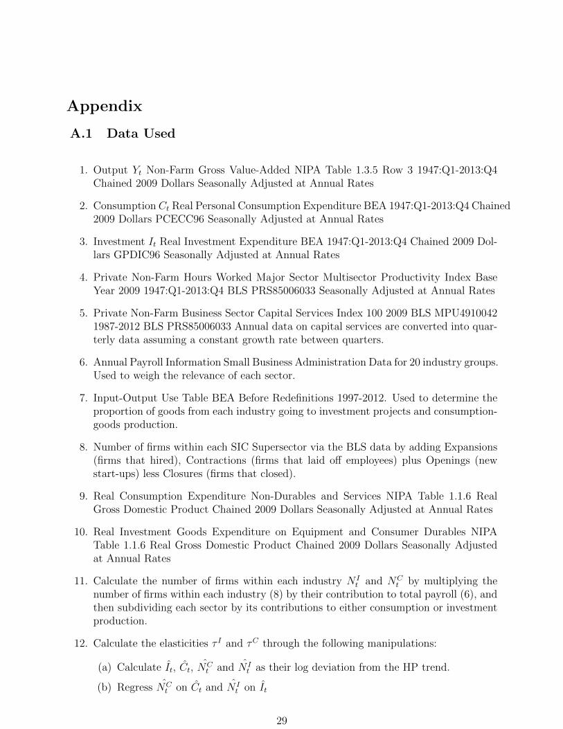
Appendix

A.1 Data Used

1. Output Yt Non-Farm Gross Value-Added NIPA Table 1.3.5 Row 3 1947:Q1-2013:Q4Chained 2009 Dollars Seasonally Adjusted at Annual Rates

2. Consumption Ct Real Personal Consumption Expenditure BEA 1947:Q1-2013:Q4 Chained2009 Dollars PCECC96 Seasonally Adjusted at Annual Rates

3. Investment It Real Investment Expenditure BEA 1947:Q1-2013:Q4 Chained 2009 Dol-lars GPDIC96 Seasonally Adjusted at Annual Rates

4. Private Non-Farm Hours Worked Major Sector Multisector Productivity Index BaseYear 2009 1947:Q1-2013:Q4 BLS PRS85006033 Seasonally Adjusted at Annual Rates

5. Private Non-Farm Business Sector Capital Services Index 100 2009 BLS MPU49100421987-2012 BLS PRS85006033 Annual data on capital services are converted into quar-terly data assuming a constant growth rate between quarters.

6. Annual Payroll Information Small Business Administration Data for 20 industry groups.Used to weigh the relevance of each sector.

7. Input-Output Use Table BEA Before Redefinitions 1997-2012. Used to determine theproportion of goods from each industry going to investment projects and consumption-goods production.

8. Number of firms within each SIC Supersector via the BLS data by adding Expansions(firms that hired), Contractions (firms that laid off employees) plus Openings (newstart-ups) less Closures (firms that closed).

9. Real Consumption Expenditure Non-Durables and Services NIPA Table 1.1.6 RealGross Domestic Product Chained 2009 Dollars Seasonally Adjusted at Annual Rates

10. Real Investment Goods Expenditure on Equipment and Consumer Durables NIPATable 1.1.6 Real Gross Domestic Product Chained 2009 Dollars Seasonally Adjustedat Annual Rates

11. Calculate the number of firms within each industry N It and NC

t by multiplying thenumber of firms within each industry (8) by their contribution to total payroll (6), andthen subdividing each sector by its contributions to either consumption or investmentproduction.

12. Calculate the elasticities τ I and τC through the following manipulations:

(a) Calculate It, Ct, NCt and N I

t as their log deviation from the HP trend.

(b) Regress NCt on Ct and N I

t on It

29

(c) Using the conditions

Ct =(τC(µC − 1))

(1− τC)NCt (94)

It =(τ I(µI − 1))

(1− τ I)N It , (95)

and set µI = µC = 1.3 and calculate values τC and τ I .

13. Calculate µCt and µIt by equations

µCt =(1− τCµC)

(τCµC)Ct (96)

µIt =(1− τ IµI)

(τ IµI)It. (97)

30

Table 1Precursor OLS Estimates for τC τ I

Sector Consumption Investment

Theory NCt =

(1−τC

τC(µC−1)

)Ct N I

t =(

1−τIτI(µI−1)

)It

Data NCt =

−6.745e−19

(0.001)+

1.123***(0.11)

Ct N It =

−3.66e−19

(0.001)+

0.394***(0.027)

It

R2 0.5648 0.7252

Note: Data on both the dependent and independent variables are outlined in the appendix. Each variableaccompanied by a hat is the log deviation from its Hodrick–Prescott filter trend, where λ = 1600 with nodrift. Data ranges from 1992Q3 to 2013Q4. Significance codes: ’***’ denotes 0.001, ’**’ 0.01, and ’*’ 0.05.

Table 2Priors

Parameter Prior Distribution Lower Bound Upper Bound Mean Varianceτ I Normal 0.90 0.05τC Normal 0.78 0.05θ Gamma 3 0.75χ Beta 0.5 0.1η Uniform 0.01 0.99hss Normal 0.3 0.03ρZ Beta 0.9 0.05ρA Beta 0.9 0.05ρv Beta 0.9 0.05ρb Beta 0.9 0.05ρµw Beta 0.9 0.05ρµZ Beta 0.40 0.20ρµA Beta 0.20 0.10σi Inv gamma 0.5 2σk Uniform 0 1

4σobs

Note: σi refers to the variance of an unanticipated shock to i = {Z,A, b, V, µW , µZ , µA}, and σk the varianceof the measurement error for the observable k = {Y, I, C,H,RPI}.

31

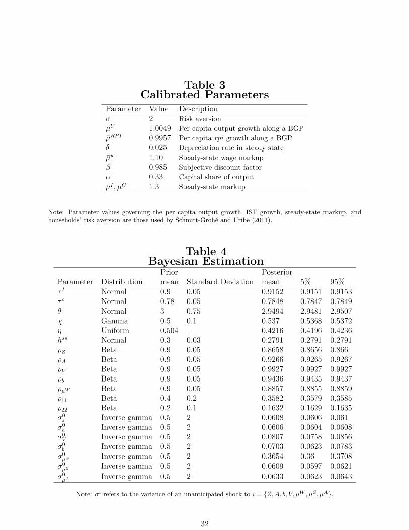
Table 3Calibrated Parameters

Parameter Value Descriptionσ 2 Risk aversion

µY 1.0049 Per capita output growth along a BGP

µRPI 0.9957 Per capita rpi growth along a BGP

δ 0.025 Depreciation rate in steady state

µw 1.10 Steady-state wage markup

β 0.985 Subjective discount factor

α 0.33 Capital share of output

µI , µC 1.3 Steady-state markup

Note: Parameter values governing the per capita output growth, IST growth, steady-state markup, andhouseholds’ risk aversion are those used by Schmitt-Grohe and Uribe (2011).

Table 4Bayesian Estimation

Prior PosteriorParameter Distribution mean Standard Deviation mean 5% 95%τ I Normal 0.9 0.05 0.9152 0.9151 0.9153τ c Normal 0.78 0.05 0.7848 0.7847 0.7849θ Normal 3 0.75 2.9494 2.9481 2.9507χ Gamma 0.5 0.1 0.537 0.5368 0.5372η Uniform 0.504 − 0.4216 0.4196 0.4236hss Normal 0.3 0.03 0.2791 0.2791 0.2791ρZ Beta 0.9 0.05 0.8658 0.8656 0.866ρA Beta 0.9 0.05 0.9266 0.9265 0.9267ρV Beta 0.9 0.05 0.9927 0.9927 0.9927ρb Beta 0.9 0.05 0.9436 0.9435 0.9437ρµW Beta 0.9 0.05 0.8857 0.8855 0.8859ρ11 Beta 0.4 0.2 0.3582 0.3579 0.3585ρ22 Beta 0.2 0.1 0.1632 0.1629 0.1635σ0z Inverse gamma 0.5 2 0.0608 0.0606 0.061σ0a Inverse gamma 0.5 2 0.0606 0.0604 0.0608σ0V Inverse gamma 0.5 2 0.0807 0.0758 0.0856σ0b Inverse gamma 0.5 2 0.0703 0.0623 0.0783σ0µw Inverse gamma 0.5 2 0.3654 0.36 0.3708σ0µZ Inverse gamma 0.5 2 0.0609 0.0597 0.0621

σ0µA Inverse gamma 0.5 2 0.0633 0.0623 0.0643

Note: σi refers to the variance of an unanticipated shock to i = {Z,A, b, V, µW , µZ , µA}.

32

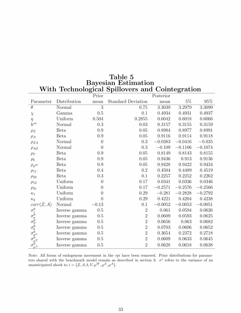
Table 5Bayesian Estimation

With Technological Spillovers and CointegrationPrior Posterior

Parameter Distribution mean Standard Deviation mean 5% 95%θ Normal 3 0.75 3.3039 3.2979 3.3099χ Gamma 0.5 0.1 0.4934 0.4931 0.4937η Uniform 0.504 0.2855 0.6042 0.6018 0.6066hss Normal 0.3 0.03 0.3157 0.3155 0.3159ρZ Beta 0.9 0.05 0.8984 0.8977 0.8991ρA Beta 0.9 0.05 0.9116 0.9114 0.9118ρZA Normal 0 0.3 −0.0383 −0.0416 −0.035ρAZ Normal 0 0.3 −0.109 −0.1106 −0.1074ρV Beta 0.9 0.05 0.8149 0.8143 0.8155ρb Beta 0.9 0.05 0.9436 0.913 0.9136ρµW Beta 0.9 0.05 0.9428 0.9422 0.9434ρ11 Beta 0.4 0.2 0.4504 0.4489 0.4519ρ22 Beta 0.3 0.1 0.2257 0.2252 0.2262ρ12 Uniform 0 0.17 0.0341 0.0336 0.0346ρ21 Uniform 0 0.17 −0.2571 −0.2576 −0.2566κ1 Uniform 0 0.29 −0.281 −0.2828 −0.2792κ2 Uniform 0 0.29 0.4221 0.4204 0.4238corr(Z,A) Normal −0.13 0.1 −0.0052 −0.0053 −0.0051σ0z Inverse gamma 0.5 2 0.061 0.0594 0.0626σ0a Inverse gamma 0.5 2 0.0609 0.0593 0.0625σ0V Inverse gamma 0.5 2 0.0656 0.063 0.0682σ0b Inverse gamma 0.5 2 0.0703 0.0606 0.0652σ0µw Inverse gamma 0.5 2 0.3654 0.2372 0.2718σ0µZ Inverse gamma 0.5 2 0.0609 0.0633 0.0645

σ0µA Inverse gamma 0.5 2 0.0628 0.0618 0.0638

Note: All forms of endogenous movement in the rpi have been removed. Prior distributions for parame-ters shared with the benchmark model remain as described in section 3. σi refers to the variance of anunanticipated shock to i = {Z,A, b, V, µW , µZ , µA}.

33

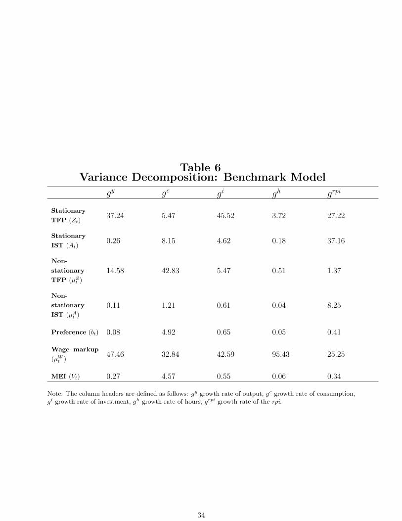
Table 6Variance Decomposition: Benchmark Model

gy gc gi gh grpi

Stationary

TFP (Zt)37.24 5.47 45.52 3.72 27.22

Stationary

IST (At)0.26 8.15 4.62 0.18 37.16

Non-

stationary

TFP (µZt )

14.58 42.83 5.47 0.51 1.37

Non-

stationary

IST (µAt )

0.11 1.21 0.61 0.04 8.25

Preference (bt) 0.08 4.92 0.65 0.05 0.41

Wage markup

(µWt )47.46 32.84 42.59 95.43 25.25

MEI (Vt) 0.27 4.57 0.55 0.06 0.34

Note: The column headers are defined as follows: gy growth rate of output, gc growth rate of consumption,gi growth rate of investment, gh growth rate of hours, grpi growth rate of the rpi.

34

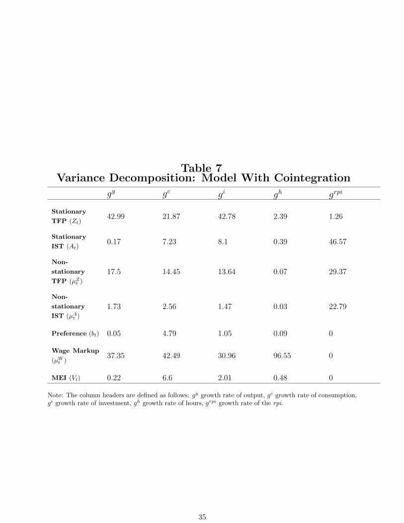
Table 7Variance Decomposition: Model With Cointegration

gy gc gi gh grpi

Stationary

TFP (Zt)42.99 21.87 42.78 2.39 1.26

Stationary

IST (At)0.17 7.23 8.1 0.39 46.57

Non-

stationary

TFP (µZt )

17.5 14.45 13.64 0.07 29.37

Non-

stationary

IST (µAt )

1.73 2.56 1.47 0.03 22.79

Preference (bt) 0.05 4.79 1.05 0.09 0

Wage Markup

(µWt )37.35 42.49 30.96 96.55 0

MEI (Vt) 0.22 6.6 2.01 0.48 0

Note: The column headers are defined as follows: gy growth rate of output, gc growth rate of consumption,gi growth rate of investment, gh growth rate of hours, grpi growth rate of the rpi.

35

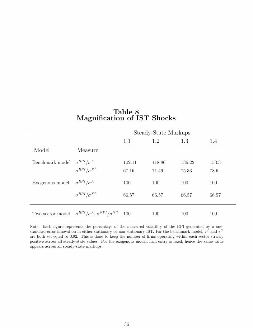
Table 8Magnification of IST Shocks

Steady-State Markups

1.1 1.2 1.3 1.4

Model Measure

Benchmark model σRPI/σA 102.11 118.86 136.22 153.3

σRPI/σXA

67.16 71.49 75.33 78.6

Exogenous model σRPI/σA 100 100 100 100

σRPI/σXA

66.57 66.57 66.57 66.57

Two-sector model σRPI/σA, σRPI/σXA

100 100 100 100

Note: Each figure represents the percentage of the measured volatility of the RPI generated by a one-standard-error innovation in either stationary or non-stationary IST. For the benchmark model, τ I and τC

are both set equal to 0.92. This is done to keep the number of firms operating within each sector strictlypositive across all steady-state values. For the exogenous model, firm entry is fixed, hence the same valueappears across all steady-state markups.

36

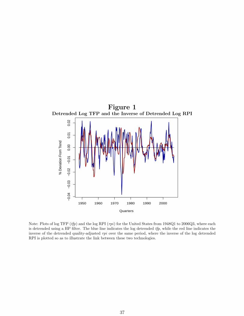
Figure 1Detrended Log TFP and the Inverse of Detrended Log RPI

1950 1960 1970 1980 1990 2000

−0.0

4−0

.03

−0.0

2−0

.01

0.00

0.01

0.02

Quarters

% D

evia

tion

From

Tre

nd

Note: Plots of log TFP (tfp) and the log RPI (rpi) for the United States from 1948Q1 to 2006Q3, where eachis detrended using a HP filter. The blue line indicates the log detrended tfp, while the red line indicates theinverse of the detrended quality-adjusted rpi over the same period, where the inverse of the log detrendedRPI is plotted so as to illustrate the link between these two technologies.

37

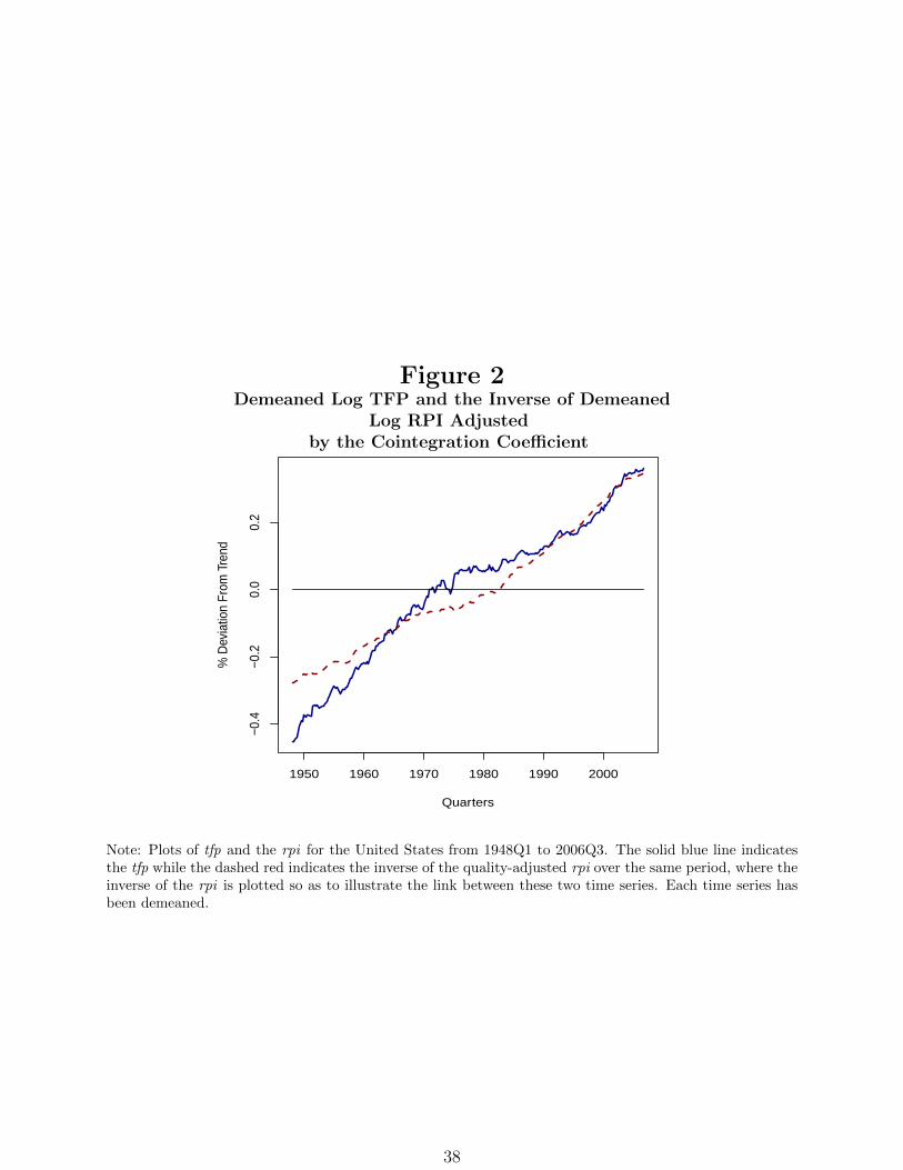
Figure 2Demeaned Log TFP and the Inverse of Demeaned

Log RPI Adjustedby the Cointegration Coefficient

1950 1960 1970 1980 1990 2000

−0.4

−0.2

0.0

0.2

Quarters

% D

evia

tion

From

Tre

nd

Note: Plots of tfp and the rpi for the United States from 1948Q1 to 2006Q3. The solid blue line indicatesthe tfp while the dashed red indicates the inverse of the quality-adjusted rpi over the same period, where theinverse of the rpi is plotted so as to illustrate the link between these two time series. Each time series hasbeen demeaned.

38

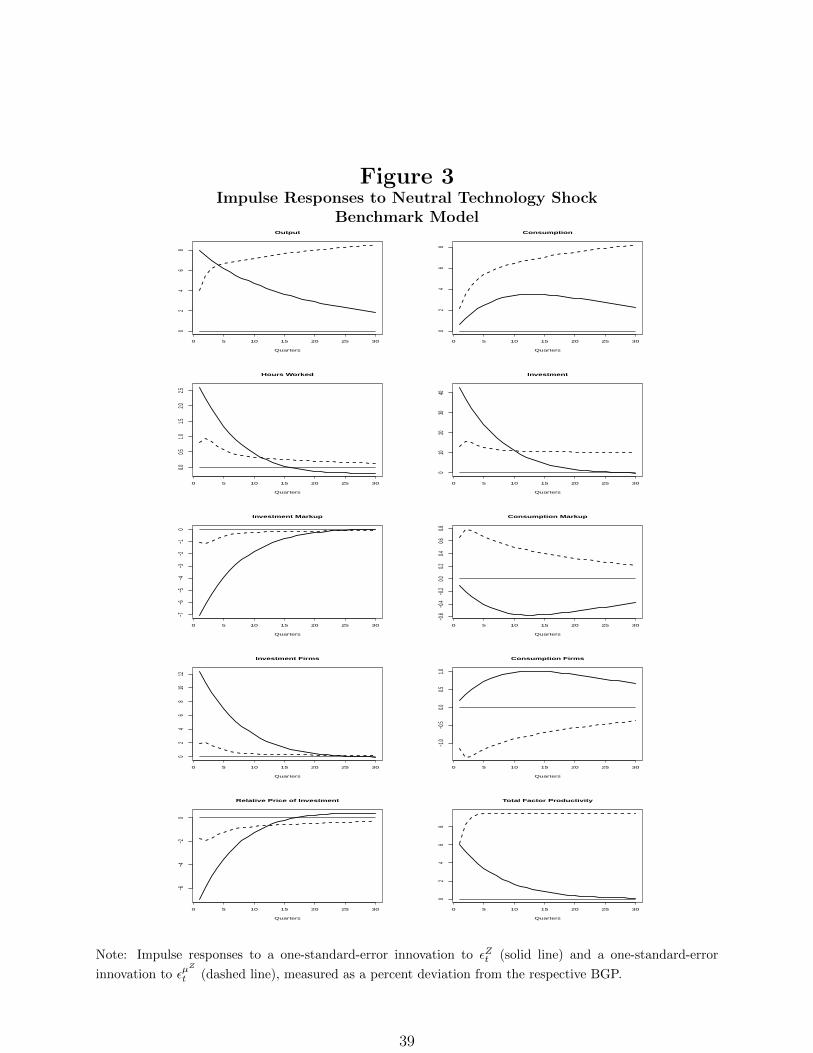
Figure 3Impulse Responses to Neutral Technology Shock

Benchmark Model

0 5 10 15 20 25 30

02

46

8

Output

Quarters

0 5 10 15 20 25 30

02

46

8

Consumption

Quarters

0 5 10 15 20 25 30

0.00.5

1.01.5

2.02.5

Hours Worked

Quarters

0 5 10 15 20 25 30

010

2030

40

Investment

Quarters

0 5 10 15 20 25 30

−7−6

−5−4

−3−2

−10

Investment Markup

Quarters

0 5 10 15 20 25 30

−0.6

−0.4

−0.2

0.00.2

0.40.6

0.8

Consumption Markup

Quarters

0 5 10 15 20 25 30

02

46

810

12

Investment Firms

Quarters

0 5 10 15 20 25 30

−1.0

−0.5

0.00.5

1.0

Consumption Firms

Quarters

0 5 10 15 20 25 30

−6−4

−20

Relative Price of Investment

Quarters

0 5 10 15 20 25 30

02

46

8

Total Factor Productivity

Quarters

Note: Impulse responses to a one-standard-error innovation to εZt (solid line) and a one-standard-error

innovation to εµZ

t (dashed line), measured as a percent deviation from the respective BGP.

39

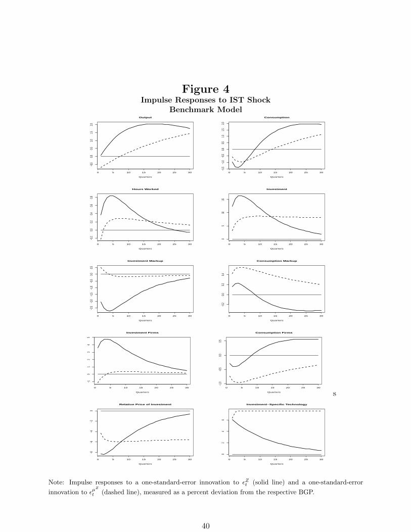
Figure 4Impulse Responses to IST Shock

Benchmark Model

0 5 10 15 20 25 30

−0.5

0.00.5

1.01.5

2.0

Output

Quarters

0 5 10 15 20 25 30

−1.5

−1.0

−0.5

0.00.5

1.01.5

2.0

Consumption

Quarters

0 5 10 15 20 25 30

−0.2

0.00.2

0.40.6

0.8

Hours Worked

Quarters

0 5 10 15 20 25 30

05

1015

Investment

Quarters

0 5 10 15 20 25 30

−2.5

−2.0

−1.5

−1.0

−0.5

0.00.5

Investment Markup

Quarters

0 5 10 15 20 25 30

−0.2

0.00.2

0.4

Consumption Markup

Quarters

0 5 10 15 20 25 30

−10

12

34

5

Investment Firms

Quarters

0 5 10 15 20 25 30

−1.0

−0.5

0.00.5

Consumption Firms

Quarters s

0 5 10 15 20 25 30

−8−6

−4−2

0

Relative Price of Investment

Quarters

0 5 10 15 20 25 30

02

46

Investment−Specific Technology

Quarters

Note: Impulse responses to a one-standard-error innovation to εZt (solid line) and a one-standard-error

innovation to εµZ

t (dashed line), measured as a percent deviation from the respective BGP.

40

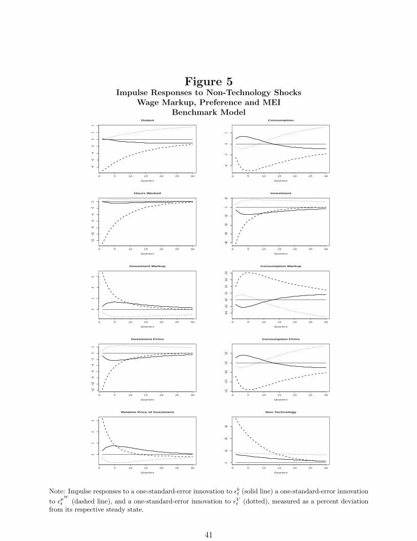
Figure 5Impulse Responses to Non-Technology Shocks

Wage Markup, Preference and MEIBenchmark Model

0 5 10 15 20 25 30

−8−6

−4−2

02

4

Output

Quarters

0 5 10 15 20 25 30

−4−2

02

Consumption

Quarters

0 5 10 15 20 25 30

−12

−10

−8−6

−4−2

0

Hours Worked

Quarters

0 5 10 15 20 25 30

−40

−30

−20

−10

010

Investment

Quarters

0 5 10 15 20 25 30

02

46

Investment Markup

Quarters

0 5 10 15 20 25 30

−0.4

−0.2

0.00.2

0.40.6

0.8

Consumption Markup

Quarters

0 5 10 15 20 25 30

−12

−10

−8−6

−4−2

02

Investment Firms

Quarters

0 5 10 15 20 25 30

−1.5

−1.0

−0.5

0.00.5

Consumption Firms

Quarters

0 5 10 15 20 25 30

02

46

Relative Price of Investment

Quarters

0 5 10 15 20 25 30

010

2030

Non Technology

Quarters

Note: Impulse responses to a one-standard-error innovation to εbt (solid line) a one-standard-error innovation

to εµW

t (dashed line), and a one-standard-error innovation to εVt (dotted), measured as a percent deviationfrom its respective steady state.

41