THE EMPIRICS OF THE SOLOW GROWTH MODEL: M B -F , R … · Mankiw, Romer, and Weil (1992) assume g is the same for all countries, so gt is the deterministic trend and ln ( A(0) ) =

31THE EMPIRICS OF THE SOLOW GROWTH MODEL

Journal of Applied Economics, Vol. VIII, No. 1 (May 2005), 31-51

THE EMPIRICS OF THE SOLOW GROWTH MODEL:LONG-TERM EVIDENCE

MILTON BAROSSI-FILHO , RICARDO GONÇALVES SILVA ,AND ELIEZER MARTINS DINIZ *

Department of Economics − FEA-RP

University of São Paulo − USP

Submitted November 2003; accepted July 2004

In this paper we reassess the standard Solow growth model, using a dynamic panel dataapproach. A new methodology is chosen to deal with this problem. First, unit root tests forindividual country time series were run. Second, panel data unit root and cointegrationtests were performed. Finally, the panel cointegration dynamics is estimated by (DOLS)method. The resulting evidence supports roughly one-third capital share in income, α.

JEL classification codes: O47, O50, O57, C33, and C52

Key words: Economic growth, panel data, unit root, cointegration and

convergence

I. Introduction

The basic Solow growth model postulates stable equilibrium with a long-

run constant income growth rate. The neoclassical assumption of analytical

representation of the production function usually consists of constant returns

to scale, Inada conditions, and diminishing returns on all inputs and some

* Ricardo Gonçalves Silva (corresponding author):. Major José Ignacio 3985, São Carlos- SP, Brazil. Postal Code: 13569-010. E-mails: [email protected], [email protected],and [email protected]. The authors acknowledge the participants of the Seventh LACEA,Uruguay, 2001; USP Academic Seminars, Brazil, 2001; XXIII Annual Meeting of theBES, Brazil, 2001 and LAMES, Brazil, 2002 for comments and suggestions on an earlierdraft. Diniz acknowledges financial support from CNPq through grant n. 301040/97-4(NV). Finally we are grateful to an anonymous referee for excellent comments whichgreatly improved the paper. All disclaimers apply.

32 JOURNAL OF APPLIED ECONOMICS

degree of substitution among them. Assuming a constant savings rate implies

that every country always follows a path along an iso-savings curve. Exogenousrates of population growth and technology were useful simplifications at thetime Solow wrote the original paper.

Despite its originality, there are some limitations in the Solow model. First,it is built on the assumption of a closed economy. That is, the convergencehypothesis supposes a group of countries having no type of interrelation.However, this difficulty can be circumvented if we argue, as Solow did, thatevery model has some untrue assumptions but may succeed if the final resultsare not sensitive to the simplifications used. In addition to the model proposedby Solow, there have been some attempts at constructing a growth model foran open economy, for example Barro, Mankiw, and Sala-I-Martin (1995).

The second limitation of the Solow model is that the implicit share ofincome that comes from capital (obtained from the estimates of the model)does not match the national accounting information. An attempt to eliminatethis problem, done by Lucas (1988), involves enlarging the concept of capitalin order to include that which is physical and human (the latter of whichconsists of education and, sometimes, health). The third limitation is that, theestimated convergence rate is too low even though attempts to modify theSolow model have impacts on this rate; e.g., Diamond model and openeconomy versions of the Ramsey-Cass-Koopmans model both have largerrates of convergence. And finally, the equilibrium rates of growth of therelevant variables depend on the rate of technological progress, an exogenousfactor and furthermore, the individuals in the Solow model (and in some ofits successors) have no motivation to invent new goods.

Notwithstanding the shortcomings mentioned, the Solow model becamethe cornerstone of economic literature focusing on the behavior of incomegrowth across countries. Moreover, the conditional convergence of incomeamong countries implies a negative correlation between the initial level ofthe real per capita GDP and the subsequent rates of growth of the samevariable. Indeed, this result arises from the assumption of diminishing returnson each input, ensuring that a less capital-intensive country tends to havehigher rates of return and, consequently, higher GDP growth rates. Detailedassessment of the convergence hypothesis and, particularly its validity acrossdifferent estimation techniques are found, inter alia, in Barro and Sala-I-

Martin (1995), Bernard and Durlauf (1996), Barro (1997) and Durlauf (2003).


The Solow neoclassical growth model was exhaustively tested in Mankiw,

Romer, and Weil (1992). They postulated that the Solow neoclassical model

fits the data better, once an additional variable - human capital - is introduced,

which improves considerably the original ability to explain income disparities

across countries. Investigating the limitations listed above, this paper uses

another route: new econometric techniques, that select a group of countries

with time series that present the same stochastic properties in order to make

reliable estimates of physical capital share. This procedure provides a new

empirical test of the Solow growth model, which yields new evidence on

income disparity behavior across countries.

Recently, the profusion of remarkable advances in econometric methods

has generated a new set of empirical tests for economic growth theories. In

keeping with this trend, an important contribution was made by Islam (1995),

whose paper reports estimates for the parameters of a neoclassical model in a

panel data approach. In this case, the author admits on leveling effects for

individual countries as heterogeneous fixed intercepts in a dynamic panel.

Although the Mankiw, Romer, and Weil (1992) findings allow us to conclude

that human capital performs an important role in the production function,

Islam (1995) reaches an opposite conclusion, once a country’s specific

technological progress is introduced into the model.

Lee, Pesaran, and Smith (1997) presented an individual random effect

version of the model, developed by Islam (1995), introducing heterogeneities

in intercepts and in slopes of the production function in a heterogeneous

dynamic panel data approach. These authors have concluded that the parameter

homogeneity hypothesis can definitely be rejected. Indeed, they point out

that different growth rates render the notion of convergence economically

meaningless, because knowledge of the convergence rate provides no insights

into the evolution of the cross-country output variance over time.

However, most classical econometric theory has been predicated on the

assumption that observed data come from stationary processes. A preliminary

glance at graphs of most economic time series or even at the historical track

record of economic forecasting is enough to invalidate that assumption, since

economies do evolve, grow, and change over time in both real and nominal

terms.


Binder and Pesaran (1999) showed that a way exists to solve this question

providing that a stochastic version of the Solow model is substituted for the

original one. This requires explicitly treating technology and labor as stochastic

processes with unit roots, which thus provide a methodological basis for using

random effects in the equations estimated in the panel data approach. Once

these settings are taking as given, Binder and Pesaran (1999) infer that the

convergence parameter estimate is interpreted purely in terms of the dynamic

random components measured in the panel data model, without any further

information about convergence dynamics itself. Binder and Pesaran (1999)

also conclude that the stochastic neoclassical growth model developed is not

necessarily a contradiction, despite the existence of unit roots in the per capita

output time series.

The purpose of this paper is threefold. First, a detailed time series analysis

is carried out on a country-by-country basis in order to build the panel. The

purpose of this procedure is to emphasize some evidence relating to unit roots

and structural breaks in the data. Based on previous results, an alternative

selection criterion is used for aggregating time series with the same features.

Finally, the original Solow growth model results are validated by estimating

the panel data model based on the procedure already described.

The remainder of the paper is organized as follows: the Solow growth

model panel data and the status of the current research is discussed in section

II. Section III considers data and sample selection issues. A country-by-country

analysis and a data set re-sampling are carrying out in section IV. Section V

contains the results for unit roots and cointegration tests for the entire panel.

The final Solow growth model, which embodies an error-correction

mechanism, is presented in section VI. In the next section, issues on the validity

and interpretation of the convergence hypothesis are discussed. Concluding

remarks are presented in section VIII.

II. Solow’s Growth Model in a Dynamic Panel Version

This section presents the basics of the Solow model and discusses the

corrections needed in order to build a dynamic panel version. The methodology

is the same as that presented by Islam (1995) and restated in Lee, Pesaran,

and Smith (1997).


Let us assume a Cobb-Douglas production function:

(1)

where Y, K, L and A denote output, physical capital stock, labor force, and

technology respectively. Capital stock change over time is given by the

following equation:

where ALKk /≡ and ,/ ALYy ≡ and s is the constant savings rate ).1,0(∈s

After taking logs on both sides of equation (1), the income per capita

steady-state is:

which is the equation obtained by Mankiw, Romer, and Weil (1992). These

authors implicitly assume that the countries are already in their current steady

state.

Apart from differences in the specific parameter values for each country,

there is an additional term, ln(A(0)) + gt in equation (3), which deserves

attention. Mankiw, Romer, and Weil (1992) assume g is the same for all

countries, so gt is the deterministic trend and ln (A(0)) = a + ε, where a is a

constant and ε is the country-specific shock. However, the same cannot be

said about A(0) since this term reflects the initial technological endowments

of an individual economy.

This point is reinforced by Islam (1995) and Lee, Pesaran, and Smith

(1997), who argue that this specification form generates loss of information

on the technological parameter dynamics. The reason for this is that the panel

data approach is the natural way to specify all shifts in the specific shock

terms for a given country, ε. In order to proceed, we assume a law of motion

for the behavior of the per capita incomes near the steady state. Let y* be the

equilibrium level for the output per effective worker, and y(t), its actual value

at time t. An approximation of y in the neighborhood of the steady state

(2)

αα −= 1))()(()()( tLtAtKtY

( ) ( ) )ln(1

ln1

)0(ln)(

)(ln δ

αα

αα ++

−−

−++=

gnsgtA

tL

tY(3)

)()(/ δ++−=∂∂

gnk

ksf

k

tk


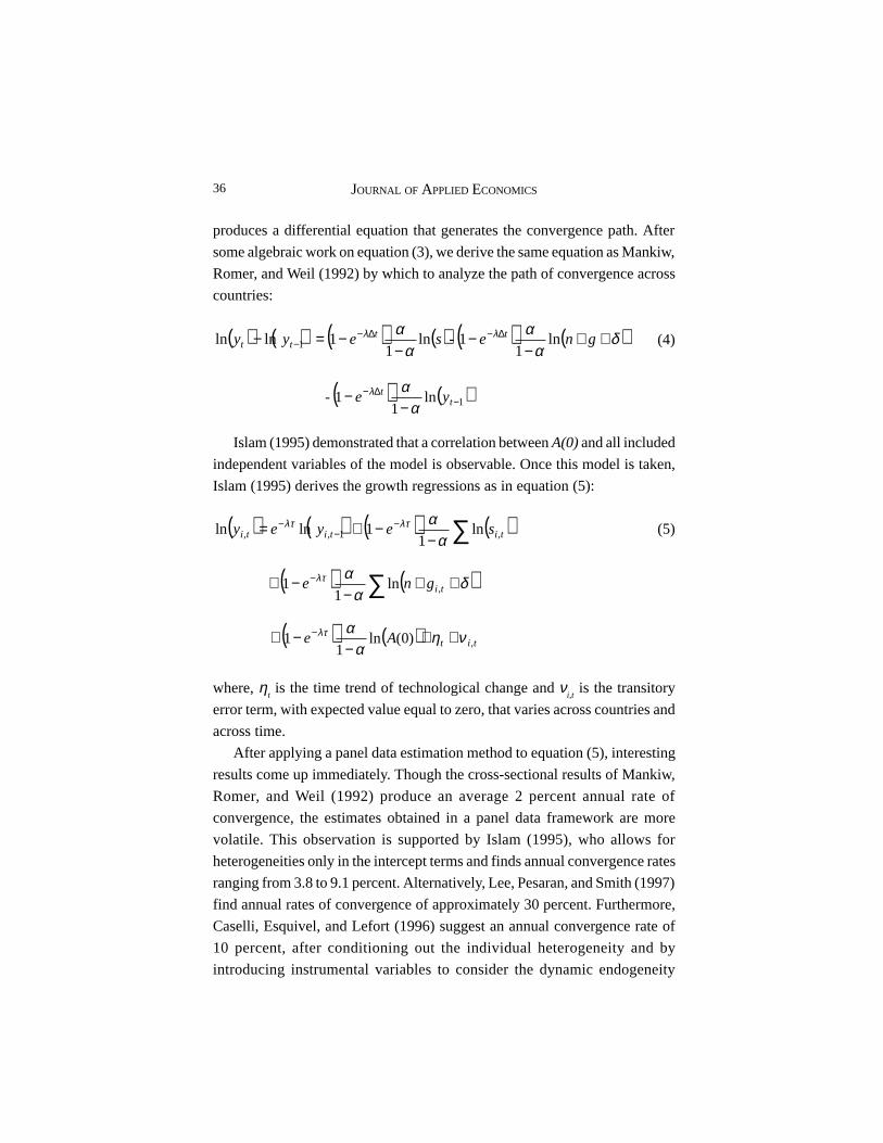
produces a differential equation that generates the convergence path. After

some algebraic work on equation (3), we derive the same equation as Mankiw,

Romer, and Weil (1992) by which to analyze the path of convergence across

countries:

Islam (1995) demonstrated that a correlation between A(0) and all included

independent variables of the model is observable. Once this model is taken,

Islam (1995) derives the growth regressions as in equation (5):

where, ηt is the time trend of technological change and ν

i,t is the transitory

error term, with expected value equal to zero, that varies across countries and

across time.

After applying a panel data estimation method to equation (5), interesting

results come up immediately. Though the cross-sectional results of Mankiw,

Romer, and Weil (1992) produce an average 2 percent annual rate of

convergence, the estimates obtained in a panel data framework are more

volatile. This observation is supported by Islam (1995), who allows for

heterogeneities only in the intercept terms and finds annual convergence rates

ranging from 3.8 to 9.1 percent. Alternatively, Lee, Pesaran, and Smith (1997)

find annual rates of convergence of approximately 30 percent. Furthermore,

Caselli, Esquivel, and Lefort (1996) suggest an annual convergence rate of

10 percent, after conditioning out the individual heterogeneity and by

introducing instrumental variables to consider the dynamic endogeneity

( ) ( ) ( ) ( ) ( ) ( )1 ln1

1-ln1

1 lnln ∆−∆−− ++

−−

−−=− tt

tt gneseyy δα

αα

α λλ

( ) ( )1ln1

1- −∆−

−− t

t yeα

αλ

(4)

( ) ( ) ( ) ( )tititi seyey ,1,, ln1

1lnlnα

αλτλτ

−−+= −

−− ∑

( ) ( )tigne ,ln1

1 δα

αλτ ++−

−+ − ∑

( ) ( ) titAe ,)0(ln1

1 νηα

αλτ ++−

−+ −

(5)


problem. Nerlove (1996), by contrast, finds annual convergence rate estimates

that are even lower then those generated by cross-section regressions. He

also argues that his findings are due to the finite sample bias of the estimator

adopted in the empirical tests of the neoclassical growth model.

Choosing a panel data approach incurs both advantages and disadvantages.1

A main disadvantage is that the nature of a panel structure as well as the

procedure of decomposition of the constant term into two additive terms and

a time-specific component does not necessarily seem theoretically natural in

many cases. However, one significant advantage comes from solving the

problem of interpreting standard cross-section regressions. In particular, the

dynamic equation typically displays correlation between lagged dependent

variables and unobservable residual, for example, the Solow residual.

Therefore, the resulting regression bias depends on the number of observations

and disappears only when that figure approaches infinity. This point is one of

the most important issues treated in this paper, mainly because it complicates

in interpreting convergence regression findings in terms of poor countries,

narrowing the gap between themselves.

Most research on this topic admits time spans in estimating the panels as

opposed to use of an entire time series (a recent exception is Ferreira, Issler,

and Pessôa (2000)). In fact, this could conceal important problems such as

unit roots and structural breaks. Moreover, as long as a first-order-integrated

stochastic process I(1) is detected for a set of time series, the possibility of a

panel data error-correction representation cannot be discarded.

Certainly this methodology leads to another puzzle, as stressed by Islam

(1995); i.e. the larger the time span, short-term disturbances may loom larger.

However, this paper deals with the time dimension of the panel in a more

precise form. All the procedures (such as specifying the right stochastic

processes underlying time series behavior) are used in order to guarantee the

absence of bias in the estimated parameters, which the most efficient strategy

in handling this problem, is to start with an individual investigation for each

time series included in the time dimension of the panel, before estimating the

panel parameters.

1 Durlauf and Quah (1999) provide a good source for supporting these arguments.


III. Data Set and Samples

Following the traditional approach in dealing with growth empirics, as in

Mankiw, Romer, and Weil (1992); Nerlove (1996); and Barro (1997), among

others, we use data on real national accounts, compiled by Heston and

Summers (1991) and known as Penn World Tables Mark 5.6. This includes

time series based on real income, real government and private investment

spending, and population growth for 1959-1989. The countries included in

our sample are described in Table 1.

Note that countries included are only the ones which compose the First-

Order Integrated Sample (IS), as described in next section.

Table 1. Countries Included in Analysis

First order stationary sample

Algeria Guinea-Bissau Papua New Guinea

Argentina Guyana Korea, Rep. of

Austria Italy Romania

Bangladesh Jamaica Russia

Belgium Jordan South Africa

Benin Kenya Sri Lanka

Bolivia Madagascar Swaziland

Botswana Mali Thailand

Burkina Faso Mauritania The Gambia

Canada Mauritius Togo

Central African, Rep. of Morocco Trinidad and Tobago

Chad Myanmar Uganda

Cyprus Namibia United States

Denmark New Zealand Yugoslavia

Domican Republic Nicaragua Zaire

Fiji Nigeria Zambia

Ghana Pakistan Zimbabwe

Greece Panama


An important issue should be considered here. Since the present goal is to

validate the standard Solow’s model, we should consider doing the same thing

with its augmented version (Mankiw, Romer, and Weil, 1992) in the same

way. The ideal procedure would be to introduce some measures of human

capital, then testing for unit root and a possible cointegration relationship

with other variables in the model. This could be done by using the Barro-Lee

education attainment dataset (Barro and Lee, 2001).

However, the data compiled by these authors consist in a panel of

observations based on five-year spans. Since the data covers 1960-1995, we

have only 8 data points, which preclude any test for unit roots, even if corrected

for small samples.

IV. Time Series Preliminary Analysis

In fact, accurate country-by-country time series analyzes has been carried

out, the first of which was performed by Nelson and Plosser (1982). Building

on these results, in this paper, we investigate the dynamic structure of the

three time series cited above for each of the 123 countries in the data set.

The first step involves running augmented Dickey and Fuller (1979) and

Phillips and Perron (1988) unit root tests. In addition, for the time series, we

suspect there is a structural break and therefore, Lee and Strazicich (2001)

unit roots tests are performed. Based on these procedures, 30 countries are

dropped from the original data set because they fail to match the integration

degree of the time series tested2 and the final and definite sample covers the

remaining 93 countries. The empirical results obtained in this paper permit

us to state the following:3

First Fact: For 20 countries out of 93, an I(2) stochastic process was adjusted.

The real per capita income fits into a first-order integrated stochastic process,

I(1), for 73 countries, which accounts for 80 percent of the sample.

Furthermore, for 20 countries out of these 73, where the per capita income

2 In fact, these countries’ time series follow a mixture of the I(1), I(2), and I(0) processes.

3 The tables containing individual country results are available upon request.


is I(1), the null hypothesis of a single endogenous structural break is not

rejected.4

Second Fact: The per capita physical capital time series, obtained using a

proxy variable defined as the sum of private and public investment spending,

is a first-order integrated stochastic process I(1), with no exceptions for

countries in the sample.

Third Fact: The growth rates of population across countries are characterized

by first-order integrated stochastic processes I(1). The calculated values for

ADF and PP tests do not allow us to reject the null hypothesis for 101 countries

in the data set. The remaining 22 time series are all stationary. Furthermore,

the same 53 countries that follow an I(1) stochastic process for real per capita

income are, in fact, contained in this sample of 101 countries.

One of the major problems related to recent empirical works on growth

models concerns the adoption of an ad hoc procedure for choosing samples

for analysis. Therefore, though choosing a specific procedure that classifies

countries into oil producers, industrialized and developed nations and others,

seems to be consistent, nothing can be said about its reliability.

Once this argument is accepted as reasonable, we select the groups based

on stochastic characteristics of the processes that drive the entire variables

behavior set. On a country-by-country basis, it is clearly possible to aggregate

countries in an entirely new binary fashion: countries where the real per capita

income growth rates are represented by a stationary process, which can include

structural breaks, and countries where these time series are integrated. This

procedure results in three samples: the First-Order Integrated Sample (IS),

the Second-Order Integrated Sample (IIS), and the Stationary Sample (SS).5

In this paper, only the first sample is admitted; research on the remaining

samples has already been carried out by the present authors.

Additionally, empirical reasoning appropriate to support this alternative

methodology. Once the conclusion that the right frame for a growth model is

4 Tables available upon request.

5 The stationary sample contains a structural break time series subset.


based on cross-sections and time-series dimensions of a panel, the next step

involves performing a panel data unit root test. Then first the existence of a

cointegration relationship among the variables that constitute the model has

to be tested for. If this relationship is supported by the data, the estimation of

an error-correction mechanism is the final step.

V. Panel Data Unit Root and Cointegration Tests

The panel data unit root test calculated is based on an original approach

incorporated in recent econometric literature. For the sake of this test, the

null hypothesis refers to non-stationary behavior of the time series, connection

admitting the possibility that the error terms are serially correlated with

different serial correlation coefficients in cross-sectional units. The test is

calculated as an averaged ADF t-statistic, as presented in Im, Pesaran, and

Shin (2002):

The calculated values of the Im, Pesaran, and Shin panel data unit root

test are reported in Table 2.

titiiiti vyty ,1,, +++= −ρβα (6)

Table 2. Panel Data Unit Root Test Estimates - IPS

Variables IPS t-test IPS LM-test

Income growth -30.6558 37.4643

Per capita income -1.8544 2.1694

Saving rates -1.0288 1.9242

Population growth 0.0869 0.9186

The null hypothesis of one unit root is rejected only in the case of the realincome growth variable. For the other four variables, the calculated unit roottest estimates are not cause for rejecting the null hypothesis. Moreover, thetest is calculated in a panel representation that accounts for a both constantterm and a time-trend component as in equation (6).


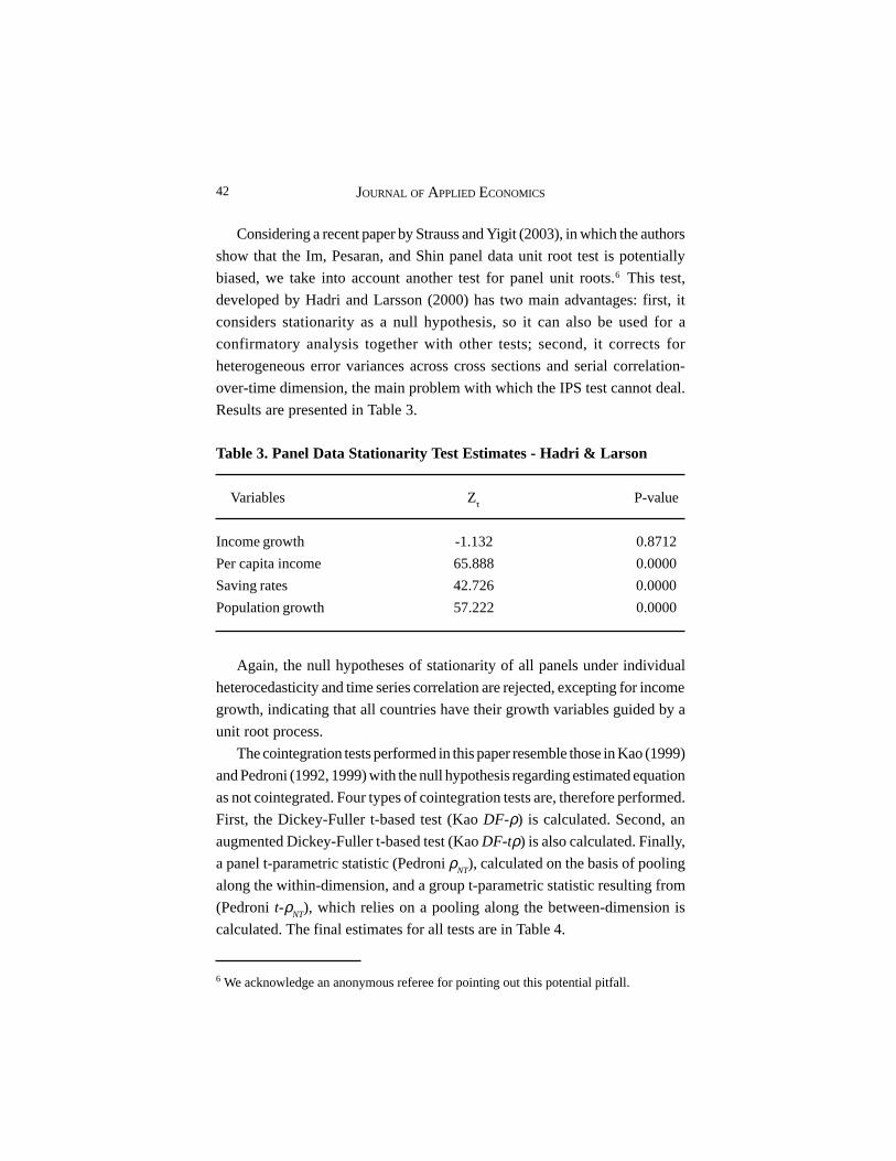
Considering a recent paper by Strauss and Yigit (2003), in which the authors

show that the Im, Pesaran, and Shin panel data unit root test is potentially

biased, we take into account another test for panel unit roots.6 This test,

developed by Hadri and Larsson (2000) has two main advantages: first, it

considers stationarity as a null hypothesis, so it can also be used for a

confirmatory analysis together with other tests; second, it corrects for

heterogeneous error variances across cross sections and serial correlation-

over-time dimension, the main problem with which the IPS test cannot deal.

Results are presented in Table 3.

6 We acknowledge an anonymous referee for pointing out this potential pitfall.

Table 3. Panel Data Stationarity Test Estimates - Hadri & Larson

Variables Zτ P-value

Income growth -1.132 0.8712

Per capita income 65.888 0.0000

Saving rates 42.726 0.0000

Population growth 57.222 0.0000

Again, the null hypotheses of stationarity of all panels under individual

heterocedasticity and time series correlation are rejected, excepting for income

growth, indicating that all countries have their growth variables guided by a

unit root process.

The cointegration tests performed in this paper resemble those in Kao (1999)

and Pedroni (1992, 1999) with the null hypothesis regarding estimated equation

as not cointegrated. Four types of cointegration tests are, therefore performed.

First, the Dickey-Fuller t-based test (Kao DF-ρ) is calculated. Second, an

augmented Dickey-Fuller t-based test (Kao DF-tρ) is also calculated. Finally,

a panel t-parametric statistic (Pedroni ρNT

), calculated on the basis of pooling

along the within-dimension, and a group t-parametric statistic resulting from

(Pedroni t-ρNT

), which relies on a pooling along the between-dimension is

calculated. The final estimates for all tests are in Table 4.


Once the estimated results for all tests proved to be significant compared

to the cut-off significance values, the null hypothesis of no cointegration was

rejected. Therefore, the next step involves the estimation of an error-correction

model for the Solow growth model, which is the main topic of discussion in

the next section.

VI. The Solow Model in an Error-Correction Presentation

The estimated error-correction model7 is based on a reparameterization

of an autoregressive distributed lag model represented by ARDL (p, q). If the

time series observations can be stacked for each group in the panel, the ECM

can be written as follows:

1i, i , ,T∀ = K where yi = (y

i,1,…,y

i,T)t is a T x 1 vector of observations on real

per capita income for the ith group of the panel; Xi = (x

i,1,…,x

i,T)t is a T x k

matrix of observations on the independent variables of the model, which vary

across groups and across time, i.e., population growth rates and per capita

physical capital accumulation rates, and D = (d1,…,d

T)t is a matrix of dimension

T x S that includes the observations on time-invariant independent variables

as intercepts and time-trend variables.

Table 4. Cointegration Test Estimates for the Solow Model

Test type Statistic Probability

Kao: D-Fρ -700.489 0.0000

Kao: D-Ftρ -409.482 0.0000

Pedroniρ -13.538 0.0000

Pedroni tρ -17.630 0.0000

7 ECM, henceforth.

iiji

p

jjiji

p

jjiiiii εγδλβφ ++∆+∆++=∆ −

−

=−

−

=− ∑∑ DXyXyy ,

1

1

*,,

1

1

*,1, (7)


Assuming that disturbances are identical and independently distributed

across countries and over time, and that the roots of the ARDL model are

outside the unit circle, it is possible to ensure that there exists a long-run

relationship between yi,T

and xi,T

, defined by the following equation:

where the error term, ηi,t, is a stationary process. Clearly, we conclude that

the order of integration of the variable yi,t is, at most, equal to the order of

integration of the regressors.

In order to write equation (7) in a more compact and intuitive manner, we

set the long-run coefficients on Xi,t as θ

i = β

i / φ

i to be the same across groups,

namely θi = θ, which results the ECM expression:

where , 1( )i i iξ θ θ−= −y X

is the error-correction component of the entire ECM representation.

The introduction of dynamic panel data methodology affects the traditional

analysis of growth model. Due to the inner structure of this model, this admits

the effects of variables in levels and lags, on the estimation step. Relying on

a theoretical statistical viewpoint, the procedure is optimal, since all parameters

of the model are estimated by maximizing a likelihood function. Another

difference concerns the interpretation of short and long-run estimated

coefficients. Basically, once an error-correction model is admitted, one is

dealing with actual values, though estimating only observed long-run

parameters.

Finally, the common procedure in estimating an unrestricted and a restricted

form of the basic empirical specification, in an error-correction model allows

for different interpretations. This happens because cointegration vector

estimation is sensitive to a linear combination of the variables.

The estimated results of a dynamic fixed-effects panel model in an error-

correction form are presented in Table 5.

, , ,i

i t i t i ti

y xβ ηφ

′ = − +

(8)

( )i i i i i iφ ξ θ κ ε∆ = + +y W (9)

(10)


Table 5. Dynamic Panel Estimates for the Growth Model

Unrestricted regression

Variables Long-run coefficients

ln (s) 0.4926

(0.1435)*

ln (n + g + δ) -1.2787

(0.3565)*

φθ 0.4926

φ -0.0742

Model adjustment statistics

AIC 1,832.1600

SC 1,678.3900

LR stat. for long-run parameters 224.0441

p-value 0.0000

Restricted regression

Variables Long-run coefficients

ln (s) - ln (n + g + δ) 0.5144

(0.0420)*

Implied α 0.3396

φθ 0.5144

φ -0.0696

Model adjustment statistics

AIC 1,902.4500

SC 1,753.0000

LR stat. for long-run parameters 135.0147

p-value 0.0000

Notes: The dependent variable is ln(y). Numbers in parenthesis refer to standard deviationsand the signal * indicates significance at 5% levels. Sample size: 1,484.


Based on these, it is possible to state the following: first, the coefficient of

savings and population growth rates shows the theoretically predicted signs,

but not at the same level of magnitude. This finding apparently contradicts

the hypothesis of constant returns to scale, indicating the prevalence of

decreasing returns, since the magnitude of the effective depreciation variable

is, in the modulus, twice the magnitude of the savings rate. However, if this is

true when the restricted equation is estimated, the correct physical capital

share cannot be found.

Now, taking into account the restricted equation, the estimated parameter

provides an implicit capital share whose value is exactly one third.

Additionally, the sign of this coefficient was found to be positive. Thus, our

results support the standard view of α = 1/3, once the implied α is calculated.

In contrast to the widespread claim that the Solow model explains cross-

country variability in labor productivity largely by appealing to variations in

technologies, the two readily observable variables on which the Solow model

focuses account, in fact, for most of the variations in per capita income.

Concerning the countries’ time series which are proved to be represented

by an I(2) integrated stochastic process, an additional a concluding remark

should be added. The possible absence of diminishing returns to capital, a

key property upon which the endogenous growth theory relies, is an assumption

that many authors have provided a basis for in the recent literature. This is the

case, for example, of Lucas (1988), Romer (1990), and Rebelo (1991). Based

on the analysis in this paper, it remains an open question whether this sort of

endogenous growth models are sufficient to explain the dynamic behavior of

economies whose income growth stochastic process embodies an acceleration

property.

Setting up a simple endogenous growth model, such as the AK model,8

we can easily observe the absence of diminishing returns to capital. An

economy described by this model can display positive long-run per capita

growth without any technological progress, which is coherent with the presence

of an embodied acceleration component.

8 Like Barro and Sala-I-Martin (1995), we also think that the first economist to use aproduction function of the AK type was Von Neumann (1937).


Many authors, including Barro and Sala-I-Martin (1995) and those citedin their references therein, mention that one way to think about the absenceof diminishing returns to capital in the AK production function is to considera broad concept of capital encompassing both physical and human components.Unfortunately, as pointed out in section III, there is no appropriate data forcarrying out an econometric analysis based on the approach presented here.Thus, such new other ideas as learning-by-doing, discussed by Arrow (1962)and Romer (1990), and purposeful activity, such as R&D expenditures, as inRomer (1987), and Aghion and Howitt (1998), should be considered. Finally,concerning convergence, unlike the neoclassical model, the AK formulationdoes not predict absolute or conditional convergence, which constitutes asubstantial failing of the model, because conditional convergence appears tobe an empirical regularity. This is certainly a matter for further research.

VII. Interpreting Convergence

Interpreting income convergence hypotheses by panel data estimation is acontroversial issue, because it centers on the interpretation of estimated speedof convergence and, consequently, its validity.

In Bernard and Durlauf (1996), the authors argue that cross-sectionalconvergence tests, as performed by Mankiw, Romer, and Weil (1992) andothers are based on the fact that data are in transition towards a limiting

distribution and, therefore, the convergence hypothesis must be interpretedas a catching-up. The same reasoning should be applied to a panel dataapproach. Furthermore, the authors arrogate that time series tests assume thatdata sets are generated by economies near their limiting distributions, andconvergence must be interpreted to mean that initial conditions have no effecton the expected value of output differences across countries. Consequently, agiven approach is appropriate depending upon whether one regards the dataas better fitting by transition or steady state dynamics.

In this paper, the estimation of an ECM provides us with a framework tointerpret convergence by either type of dynamics without violating Proposition6 in Bernard and Durlauf (1996). First, concerning cross-sectional and paneldata tests, we found that the expected value of growth income across countries

is negative while the difference between initial incomes is positive. At the

same time, the existence of an error correction term, φ, implies that in the


long run, the system is I(0), so that absence of unit roots is consistent with the

convergence hypothesis under the time series structure of the model.

In this fashion, the long-run behavior of income across countries furnishes

us with a proxy for the speed of convergence, i.e. the error correction term.

In our model, this term assumes the value of 0.0742. In other words, economies,

on the average, will converge at a 7.42 % rate, a more reasonable result than

the usual 2 % rate.

VIII. Concluding Remarks

This paper rests on empirical evidence obtained to support the original

Solow growth model, which in fact happens, since the implied capital share

on output is approximately the same as that predicted by given national

accounting data. Furthermore, this finding on the share of capital output allows

us to arrive at larger and less restrictive conditional coefficient of the speed

of convergence.

The dynamic fixed-effects Solow growth model provides a tight theoretical

framework within which to interpret the stochastic process behind income

growth. Once the nature of stochastic processes is taken into account, an

important issue arises when estimating the long-run behavior of income growth

that is not significantly different from the predictions of the Solow model,

including the evidence for diminishing returns to scale. Since panel data the

cointegration technique assigns a fixed effect to allow for country-specific

heterogeneities, conditional convergence does not lose its meaning.

In order to apply a panel data cointegration technique, a panel unit root

test is calculated the result obtained does not allow us to reject the null

hypothesis. Therefore, an error correction model representation is estimated

following the usual time series procedure. Though an immediate comparison

to a single time series error correction representation is not direct, it is

reasonable to assume the estimated coefficient for φ is equivalent of the error

correction term, i.e., the speed of convergence.

Admittedly, our procedure is not complete. This is so because the selection

criterion suggested in this paper does not apply to when all countries are

included in the sample. However, this is a solvable problem, since recent

developments in econometric techniques deal with this problem.


Moreover, a new branch of research is open on the empirics of the Solow

growth model, mainly for those countries manifesting the existence of

structural breaks and multiple unit roots in the stochastic processes generating

their income paths.

References

Aghion, Phillip, and Peter Howitt (1998), Endogenous Growth Theory,

Cambridge, MA, MIT Press.

Arrow, Kenneth (1962), “The Economic Implications of Learning by Doing,”

Review of Economic Studies 29: 155-73.

Barro, Robert, and Jong-Wha Lee (2001), “International Data on Educational

Attainment: Updates and Implications,” Oxford Economic Papers 53:

541–63.

Barro, Robert J. (1997), Determinants of Economic Growth, Cambridge, MA,

MIT Press.

Barro, Robert. J., N. Gregory Mankiw, and Xavier Sala-I-Martin (1995),

“Capital Mobility in Neoclassical Models of Growth,” American

Economic Review 85: 103-15.

Barro, Robert J., and Xavier Sala-I-Martin (1995), Economic Growth, New

York, NY, McGraw Hill.

Bernard, Andrew B., and Steven N. Durlauf (1996), “Interpreting Tests of

the Convergence Hypothesis,” Journal of Econometrics 71: 161-73.

Binder, Michael, and M. Hashem Pesaran (1999), “Stochastic Growth Models

and their Econometric Implications,” Journal of Economic Growth 4: 139–

83.

Caselli, Francesco, Gerardo Esquivel and Fernando Lefort (1996), “Re-

opening the Convergence Debate: A New Look at Cross-country Growth

Empirics,” Journal of Economic Growth 1: 363–89.

Dickey, David A., and Wayne A. Fuller (1979), “Distribution of the Estimators

for Autoregressive Time Series with a Unit Root,” Journal of the American

Statistical Association 74: 427–31.

Durlauf, Steven (2003), “The Convergence Hypothesis after 10 Years,”

unpublished manuscript, University of Wisconsin.


Durlauf, Steven, and D. Quah (1999), The New Empirics of Economic

Growth, North Holland, Amsterdam, NL.Ferreira, Pedro C., João V. Issler, and Samuel A. Pessôa (2000), “On the

Nature of Income Inequality across Nations,” unpublished manuscript,Getúlio Vargas Foundation.

Hadri, Kadoour, and Rolf Larsson (2000), “Testing for Stationarity inHeterogeneous Panel Data where the Time Dimension is Finite,”unpublished manuscript, Liverpool University.

Heston, Alan, and Robert Summers (1991), “The Penn World Table Mark 5:An Extended Set of International Comparisons, 1950-1988,” Quarterly

Journal of Economics 106: 327–368.Im, Kyung So, M. Hashem Pesaran, and Yongcheol Shin (2003), “Testing

for Unit Roots in Heterogeneous Panels,” Journal of Econometrics 115:53-74.

Islam, Nazrul (1995), “Growth Empirics: A Panel data Approach,” QuarterlyJournal of Economics 90: 1127–1170.

Kao, Chiwa (1999), “Spurious Regression and Residual Based Tests forCointegration in Panel Data,” Journal of Econometrics 90: 1–44.

Lee, Junsoo, and Mark Strazicich (2001), “Break Point Estimation andSpurious Rejections with Endogenous Unit Root Tests,” Oxford Bulletinof Economics and Statistics 63: 535–558.

Lee, Kevin, M. Hashem Pesaran, and Ronald P. Smith (1997), “Growth andConvergence in a Multi-country Empirical Stochastic Solow Model,”Journal of Applied Econometrics 12: 357–392

Lucas, Robert E. (1988), “On the Mechanics of Economic Development,”Journal of Monetary Economics 22: 3–42.

Mankiw, N. Greogory, David Romer, and David N. Weil (1992), “AContribution to the Empirics of Economic Growth,” Quarterly Journal of

Economics 58: 407–437.Nelson, Charles R., and Charles I. Plosser (1982), “Trends and Random Walks

in Economic Time Series,” Journal of Monetary Economics 10: 139–162.Nerlove, Mark (1996), “Growth Rate Convergence: Fact or Artifact?”,

unpublished manuscript, University of Maryland.

Pedroni, Peter (1992), “Panel Cointegration: Asymptotic and Finite Sample

Properties of Pooled Time Series Tests with an Application to the PPP

Hypothesis,” forthcoming in Econometric Theory.


Pedroni, Peter (1999), “Critical Values for Cointegration Tests in

Heterogeneous Panels with Multiple Regressors,” Oxford Bulletin of

Economics and Statistics 16: 653–678.

Phillips, Peter C. B., and Pierre Perron (1988), “Testing for a Unit Root in

Time Series Regression,” Biometrika 75: 335–346.

Rebelo, Sergio (1991), “Long Run Policy Analysis and Long Run Growth,”

Journal of Political Economy 99: 500–521.

Romer, Paul (1987), “Growth Based on Increasing Returns Due to

Specialization,” American Economic Review 78: 56–62.

Romer, Paul M. (1990), “Endogenous Technological Change,” Journal of

Political Economy 98: 71–102.

Strauss, Jack, and Taner Yigit (2003), “Shortfalls of Panel Data Unit Root

Testing,” Economics Letters 81: 309–13.

Von Neumann, John (1937), “Uber ein Okonomishes Gleichungssystem und

eine Verallgemeinerung des Brouwershen,” Ergebnisse eines

Mathematishe Kolloquiuns 8.

Documents

THE EMPIRICS OF THE SOLOW GROWTH MODEL: M B -F , R … · Mankiw, Romer, and Weil (1992) assume g is the same for all countries, so gt is the deterministic trend and ln ( A(0) ) =