Embed Size (px)
Citation preview
arX
iv:m
ath/
0406
526v
1 [
mat
h.ST
] 2
5 Ju
n 20
04
The Annals of Statistics
2004, Vol. 32, No. 3, 1261–1288DOI: 10.1214/009053604000000355c© Institute of Mathematical Statistics, 2004
THE EMPIRICAL PROCESS ON GAUSSIAN SPHERICAL
HARMONICS
By Domenico Marinucci1 and Mauro Piccioni
Universita di Roma “Tor Vergata” and Universita di Roma “La Sapienza”
We establish weak convergence of the empirical process on thespherical harmonics of a Gaussian random field in the presence of anunknown angular power spectrum. This result suggests various Gaus-sianity tests with an asymptotic justification. The issue of testing forGaussianity on isotropic spherical random fields has recently receivedstrong empirical attention in the cosmological literature, in connec-tion with the statistical analysis of cosmic microwave backgroundradiation.
1. Introduction. In recent years an enormous amount of attention hasbeen devoted to testing for Gaussianity for spherical random fields, espe-cially in the astrophysical and cosmological literature. The empirical mo-tivation for these studies can be explained as follows. The ongoing NASAsatellite mission MAP and the forthcoming ESA mission Planck will probecosmic microwave background radiation (CMB) to an unprecedented accu-racy. CMB can be viewed as a signature of the distribution of matter andradiation in the very early universe, and as such it is expected to yield verytight constraints on physical models for the Big Bang. For the density fluc-tuations of this field, the highly popular inflationary scenario [see Peebles(1993) or Peacock (1999)] predicts a Gaussian distribution, whereas alter-native cosmological theories, such as topological defects or nonstandard in-flationary models, predict other types of behavior. The density distributionsof fluctuations are also instrumental for drawing correct inferences on thephysical constants which can be estimated from CMB radiation; indeed,point and interval estimation procedures for cosmological parameters havebeen based almost exclusively upon Gaussian assumptions, which of course
Received July 2002; revised April 2003.1Supported by MURST.AMS 2000 subject classifications. 60F17, 62G20, 62G30.Key words and phrases. Empirical processes, weak convergence, Gaussian spherical
harmonics, cosmic microwave background radiation.
This is an electronic reprint of the original article published by theInstitute of Mathematical Statistics in The Annals of Statistics,2004, Vol. 32, No. 3, 1261–1288. This reprint differs from the original inpagination and typographic detail.
1
2 D. MARINUCCI AND M. PICCIONI
need to be validated before reliable statistical inference can take place. Forthese reasons, many different Gaussianity tests were considered in the recentcosmological literature, some of them based upon the topological propertiesof Gaussian fields [Novikov, Schmalzing and Mukhanov (2000), Phillips andKogut (2001) and Dore, Colombi and Bouchet (2003)], others on higher-order cumulant spectra [Winitzki and Wu (2000) and Komatsu and Spergel(2001)].
Let T (θ,ϕ) be a random field indexed by the unit sphere S2; that is, foreach azimuth 0≤ θ ≤ π and elongation 0≤ ϕ < 2π, T (θ,ϕ) is a random vari-able defined on some probability space. Throughout this paper we assumethat T (θ,ϕ) has zero mean, finite variance, is mean square continuous, andis isotropic, that is, its covariance is invariant with respect to the group ofrotations. Furthermore, we introduce the spherical harmonics, defined by
Yl,m(θ,ϕ) =
√2l+1
4π
(l−m)!
(l+m)!Plm(cos θ) exp(imϕ), for m> 0,
(−1)mY ∗l,−m(θ,ϕ), for m< 0,
where the asterisk denotes complex conjugation and Plm(cos θ) denotes theassociated Legendre polynomial of degree l, m, that is,
Plm(x) = (−1)m(1− x2)m/2 dm
dxmPl(x),
Pl(x) =1
2ll!
dl
dxl(x2 − 1)l, m= 0,1,2, . . . , l, l= 1,2,3, . . . .
A detailed discussion of the properties of the spherical harmonics can befound, for instance, in Liboff (1998), Chapter 9, and in Varshalovich, Moskalevand Khersonskii (1988), Chapter 5. The following spectral representationholds in the mean square sense [see, e.g., Hannan (1970), Wong (1971) andLeonenko (1999)]:
T (θ,ϕ) =∞∑
l=1
l∑
m=−l
almYlm(θ,ϕ),(1)
where the triangular array {alm} represents a set of random coefficientswhich can be obtained from T (θ,ϕ) through the inversion formula
alm =
∫ 2π
0
∫ π
0T (θ,ϕ)Y ∗
lm(θ,ϕ) sinθ dθ dϕ,(2)
m= 0,±1, . . . ,±l, l= 1,2, . . . .
These coefficients are zero-mean and uncorrelated [see Wong (1971), pages253 and 254]; hence, if T (θ,ϕ) is Gaussian, as we shall always assume in thispaper, they have a complex Gaussian distribution, and they are independent
SPHERICAL EMPIRICAL PROCESS 3
over l and m≥ 0 (although al,−m = (−1)ma∗lm), with variance E|alm|2 =Cl,m= 0,±1, . . . ,±l. The sequence {Cl} denotes the angular power spectrumof the random field; we shall always assume that Cl is strictly positive forall values of l.
Our purpose in this paper is to construct Gaussianity tests based on theempirical distribution function for the triangular array of random coeffi-cients {alm}, l= 1, . . . ,L, m= 0,±1, . . . ,±l, as L→∞. In principle, expres-sion (2) can be used to recover the coefficients alm for any value of l. Inpractical applications, however, L is finite and determined by the resolutionof the experiment. For instance, the coefficients alm may be contaminatedby noise, with a decreasing signal to noise ratio as l grows. Throughout thispaper we adopt the simplifying assumption that the noise is negligible onlyfor l = 1, . . . ,L, hence the higher-order coefficients are discarded. The cur-rent status of technology in satellite missions suggests that our assumptionmay provide a reasonable approximation for L as large as several hundredsfor the ongoing NASA experiment MAP, a value which is likely to increaseto a few thousands for the forthcoming ESA experiment Planck.
Testing Gaussianity in a spherical field poses considerable extra difficultyvs. testing in Euclidean spaces, since (fixed radius) spherical fields are neverergodic. Our proposal is to consider the asymptotic behavior of the empiri-cal process on the triangular array {alm}, in the presence of infinitely manyunknown parameters {Cl}; in fact, the angular power spectrum is typicallyunknown in practice, and needs to be estimated nonparametrically fromthe data [Miller, Nichol, Genovese and Wasserman (2002) and Wasserman,Miller, Nichol, Genovese, Jang, Connolly, Moore, Schneider and the PICAGroup (2001)]. The presence of a growing sequence of estimated parametersmakes it hard to exploit the modern theory of empirical processes, as pre-sented for instance by van der Vaart and Wellner (1996) or Dudley (1999);we hence resort to a more traditional approach, based upon standard weakconvergence theorems in the Skorohod space D[0,1]2, as presented for in-stance by Bickel and Wichura (1971) or Shorack and Wellner (1986). Werefer to these works for the definition and topological properties of such aspace. For the sequel it is enough to recall that, in order to prove the weakconvergence of a sequence {KL(r,α)} of D[0,1]2-valued processes to the fieldK(r,α), we need to prove both convergence of all finite-dimensional distri-butions and tightness. For the latter we will use a sufficient criterion due toBickel and Wichura (1971).
First, for a generic “block” B = (α1, α2]× (r1, r2]⊂ [0,1]2, define the in-crements of the field KL,
KL(B) =KL(α2, r2)−KL(α2, r1)−KL(α1, r2) +KL(α1, r1).
We define two types of adjacent blocks:
4 D. MARINUCCI AND M. PICCIONI
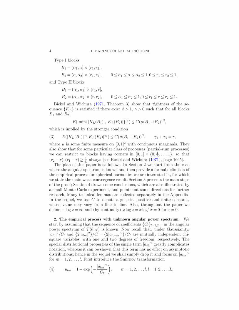
Type I blocks
B1 = (α1, α]× (r1, r2],
B2 = (α,α2]× (r1, r2], 0≤ α1 ≤ α≤ α2 ≤ 1,0≤ r1 ≤ r2 ≤ 1,
and Type II blocks
B1 = (α1, α2]× (r1, r],
B2 = (α1, α2]× (r, r2], 0≤ α1 ≤ α2 ≤ 1,0≤ r1 ≤ r ≤ r2 ≤ 1.
Bickel and Wichura (1971, Theorem 3) show that tightness of the se-quence {KL} is satisfied if there exist β > 1, γ > 0 such that for all blocksB1 and B2,
E([min{|KL(B1)|, |KL(B2)|}]γ)≤C(µ(B1 ∪B2))β,
which is implied by the stronger condition
E(|KL(B1)|γ1 |KL(B2)|γ2)≤C(µ(B1 ∪B2))β, γ1 + γ2 = γ,(3)
where µ is some finite measure on [0,1]2 with continuous marginals. Theyalso show that for some particular class of processes (partial-sum processes)we can restrict to blocks having corners in [0,1] × {0, 1L , . . . ,1}, so that
(r2 − r), (r1 − r)≥ 1L always [see Bickel and Wichura (1971), page 1665].
The plan of this paper is as follows. In Section 2 we start from the casewhere the angular spectrum is known and then provide a formal definition ofthe empirical process for spherical harmonics we are interested in, for whichwe state the main weak convergence result. Section 3 presents the main stepsof the proof; Section 4 draws some conclusions, which are also illustrated bya small Monte Carlo experiment, and points out some directions for furtherresearch. Many technical lemmas are collected separately in the Appendix.In the sequel, we use C to denote a generic, positive and finite constant,whose value may vary from line to line. Also, throughout the paper wedefine − logx=∞ and (by continuity) x logx= x log2 x= 0 for x= 0.
2. The empirical process with unknown angular power spectrum. Westart by assuming that the sequence of coefficients {Cl}l=1,2,... in the angularpower spectrum of T (θ,ϕ) is known. Now recall that, under Gaussianity,|al0|2/Cl and {2|alm|2}/Cl = {2|al,−m|2}/Cl are mutually independent chi-square variables, with one and two degrees of freedom, respectively. Thespecial distributional properties of the single term |al0|2 greatly complicatesnotation, whereas it can be shown that this term has no effect on asymptoticdistributions; hence in the sequel we shall simply drop it and focus on |alm|2for m= 1,2, . . . , l. First introduce the Smirnov transformation
ulm = 1− exp
(−|alm|2
Cl
), m= 1,2, . . . , l, l= 1,2, . . . ,L,(4)
SPHERICAL EMPIRICAL PROCESS 5
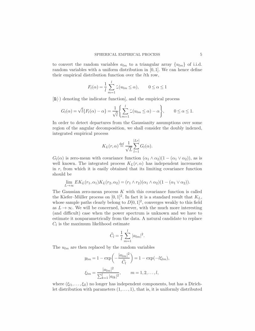
to convert the random variables alm to a triangular array {ulm} of i.i.d.random variables with a uniform distribution in [0,1]. We can hence definetheir empirical distribution function over the lth row,
Fl(α) =1
l
l∑
m=1
1(ulm ≤ α), 0≤ α≤ 1
[1(·) denoting the indicator function], and the empirical process
Gl(α) =√l{Fl(α)− α}= 1√
l
{l∑
m=1
1(ulm ≤ α)− α
}, 0≤ α≤ 1.
In order to detect departures from the Gaussianity assumptions over someregion of the angular decomposition, we shall consider the doubly indexed,integrated empirical process
KL(r,α)def=
1√L
[Lr]∑
l=1
Gl(α).
Gl(α) is zero-mean with covariance function (α1 ∧ α2)(1− (α1 ∨ α2)), as iswell known. The integrated process KL(r,α) has independent incrementsin r, from which it is easily obtained that its limiting covariance functionshould be
limL→∞
EKL(r1, α1)KL(r2, α2) = (r1 ∧ r2)(α1 ∧ α2)(1− (α1 ∨ α2)).
The Gaussian zero-mean process K with this covariance function is calledthe Kiefer–Muller process on [0,1]2. In fact it is a standard result that KL,whose sample paths clearly belong to D[0,1]2, converges weakly to this fieldas L→∞. We will be concerned, however, with the much more interesting(and difficult) case when the power spectrum is unknown and we have toestimate it nonparametrically from the data. A natural candidate to replaceCl is the maximum likelihood estimate
Cl =1
l
l∑
m=1
|alm|2.
The ulm are then replaced by the random variables
ylm = 1− exp
(−|alm|2
Cl
)= 1− exp(−lξlm),
ξlm =|alm|2
∑lk=1 |alk|2
, m= 1,2, . . . , l,
where (ξl1, . . . , ξll) no longer has independent components, but has a Dirich-let distribution with parameters (1, . . . ,1), that is, it is uniformly distributed
6 D. MARINUCCI AND M. PICCIONI
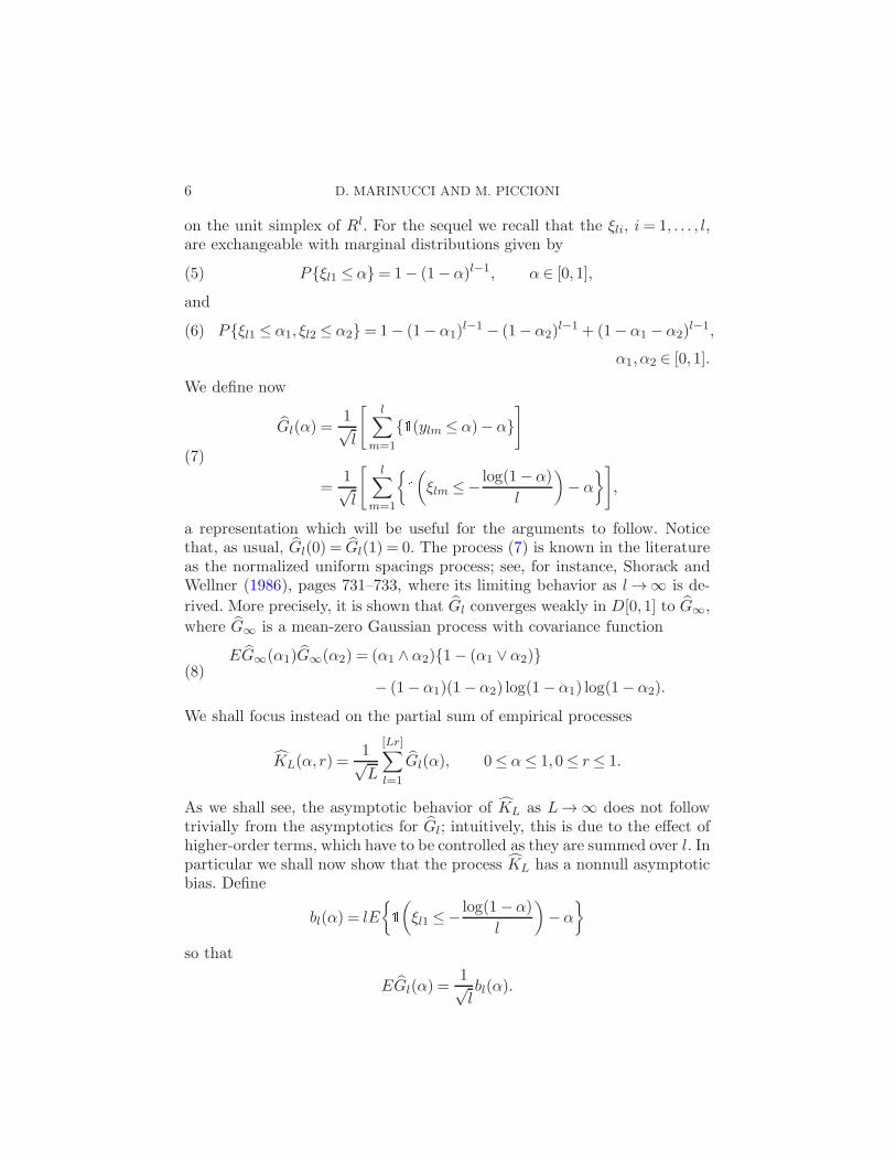
on the unit simplex of Rl. For the sequel we recall that the ξli, i= 1, . . . , l,are exchangeable with marginal distributions given by
P{ξl1 ≤ α}= 1− (1−α)l−1, α ∈ [0,1],(5)
and
P{ξl1 ≤ α1, ξl2 ≤ α2}= 1− (1− α1)l−1 − (1−α2)
l−1 + (1−α1 − α2)l−1,(6)
α1, α2 ∈ [0,1].
We define now
Gl(α) =1√l
[l∑
m=1
{1(ylm ≤ α)− α}]
(7)
=1√l
[l∑
m=1
{1
(ξlm ≤− log(1− α)
l
)− α
}],
a representation which will be useful for the arguments to follow. Noticethat, as usual, Gl(0) = Gl(1) = 0. The process (7) is known in the literatureas the normalized uniform spacings process; see, for instance, Shorack andWellner (1986), pages 731–733, where its limiting behavior as l→∞ is de-
rived. More precisely, it is shown that Gl converges weakly in D[0,1] to G∞,
where G∞ is a mean-zero Gaussian process with covariance function
EG∞(α1)G∞(α2) = (α1 ∧ α2){1− (α1 ∨ α2)}(8)
− (1−α1)(1−α2) log(1−α1) log(1− α2).
We shall focus instead on the partial sum of empirical processes
KL(α, r) =1√L
[Lr]∑
l=1
Gl(α), 0≤ α≤ 1,0≤ r≤ 1.
As we shall see, the asymptotic behavior of KL as L→∞ does not followtrivially from the asymptotics for Gl; intuitively, this is due to the effect ofhigher-order terms, which have to be controlled as they are summed over l. Inparticular we shall now show that the process KL has a nonnull asymptoticbias. Define
bl(α) = lE
{1
(ξl1 ≤− log(1−α)
l
)−α
}
so that
EGl(α) =1√lbl(α).
SPHERICAL EMPIRICAL PROCESS 7
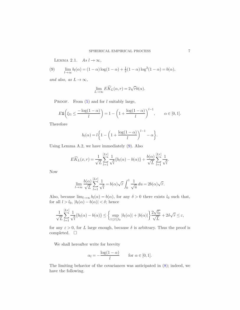
Lemma 2.1. As l→∞,
liml→∞
bl(α) = (1−α) log(1− α) + 12(1− α) log2(1− α) = b(α),(9)
and also, as L→∞,
limL→∞
EKL(α, r) = 2√rb(α).
Proof. From (5) and for l suitably large,
E1
(ξl1 ≤
− log(1−α)
l
)= 1−
(1 +
log(1−α)
l
)l−1
, α ∈ [0,1].
Therefore
bl(α) = l
{1−
(1 +
log(1−α)
l
)l−1
−α
}.
Using Lemma A.2, we have immediately (9). Also
EKL(x, r) =1√L
[Lr]∑
l=1
1√l{bl(α)− b(α)}+ b(α)√
L
[Lr]∑
l=1
1√l.
Now
liml→∞
b(α)√L
[Lr]∑
l=1
1√l= b(α)
√r
∫ 1
0
1√udu= 2b(α)
√r.
Also, because liml→∞ bl(α) = b(α), for any δ > 0 there exists l0 such that,for all l > l0, |bl(α)− b(α)|< δ; hence
1√L
[Lr]∑
l=1
1√l{bl(α)− b(α)} ≤
{sup
1≤l≤l0
|bl(α)|+ |b(α)|}2√l0√L
+2δ√r ≤ ε,
for any ε > 0, for L large enough, because δ is arbitrary. Thus the proof iscompleted. �
We shall hereafter write for brevity
αl =− log(1−α)
lfor α ∈ [0,1].
The limiting behavior of the covariances was anticipated in (8); indeed, wehave the following.
8 D. MARINUCCI AND M. PICCIONI
Lemma 2.2. For all 0≤ α1, α2 ≤ 1,
liml→∞
Cov{Gl(α1), Gl(α2)}
= (α1 ∧ α2){1− (α1 ∨ α2)}(10)
− (1− α1)(1−α2) log(1−α1) log(1−α2),
and as L→∞, for all 0≤ α1, α2 ≤ 1, 0≤ r1, r2 ≤ 1,
limL→∞
Cov{KL(α1, r1), KL(α2, r2)}
= (r1 ∧ r2)[(α1 ∧ α2){1− (α1 ∨ α2)}(11)
− (1−α1)(1−α2) log(1− α1) log(1− α2)].
Proof. The first limiting result is standard in the theory of spacings[see Shorack and Wellner (1986) and Shorack (1972)]; indeed, from (5), (6)and Lemma A.1 the reader can check that
liml→∞
Cov{1(ξl1 ≤ α1l),1(ξl1 ≤ α2l)}
= (α1 ∧ α2){1− (α1 ∨ α2)},liml→∞
lCov{1(ξl1 ≤ α1l),1(ξl2 ≤ α2l)}
=− log(1−α1) log(1−α2)(1−α1)(1− α2),
whence (10) follows easily. On the other hand, (11) is an immediate conse-quence of the Kronecker lemma and (10). �
Now write
K∗L(α, r) = KL(α, r)− 2
√rb(α),
and define K∗(α, r) as the zero-mean Gaussian process on [0,1]× [0,1] withcovariance
EK∗(α1, r1)K∗(α2, r2)
= (r1 ∧ r2)[(α1 ∧ α2){1− (α1 ∨ α2)}− (1− α1)(1−α2) log(1−α1) log(1−α2)].
To the best of our knowledge, the field K∗(α, r) has not appeared in theliterature so far, and we label it a modified Kiefer–Muller process. Our mainresult will be the following.
Theorem 2.1. As L→∞, weakly in D[0,1]2,
K∗L ⇒K∗,
⇒ denoting weak convergence in the Skorohod space D[0,1]2.
The proof of this result will be given in the next section.
SPHERICAL EMPIRICAL PROCESS 9
3. The weak convergence proof.
Proposition 3.1. As L→∞,
K∗Lf.d.d.−→K∗.
Proof. Consider 0≤ α1 < · · ·<αs ≤ 1, 0≤ r1 < · · ·< rt ≤ 1, and let
G∗l (α,β] = Gl(α,β]−EGl(α,β],(12)
for 0≤ α≤ β ≤ 1. Because of Lemma 2.1 the convergence of the s× t vectorwith components K∗
L(αi, rj) with i = 1,2, . . . , s, j = 1,2, . . . , t, to the samecomponents of K∗(α, r) is equivalent to the joint convergence of the centeredincrements
KL((αi, αi+1]× (rj, rj+1])−EKL((αi, αi+1]× (rj , rj+1])
=1√L
[Lri+1]∑
l=[Lri]+1
[Gl(αi+1)− Gl(αi)−E{Gl(αi+1)− Gl(αi)}]
=1√L
[Lri+1]∑
l=[Lri]+1
G∗l (αi, αi+1]
for i= 0, . . . , s and j = 0, . . . , t, where we have set α0 = r0 = 0, αs+1 = rt+1 =1, to the increments
K∗((αi, αi+1]× (rj, rj+1])
=K∗(αi+1, rj+1) +K∗(αi, rj)−K∗(αi, rj+1)−K∗(αi+1, rj).
Because of the independence over l we can restrict ourselves to a fixed in-terval for r, by simplicity (0,1], say. It is now clear that we have to usethe multidimensional central limit theorem (CLT) with independent but notidentically distributed summands. A suitable control on the fourth momentsclearly implies the Lindeberg condition, namely
1
L2
L∑
l=1
EG∗l (αi, αi+1]
2G∗l (αk, αk+1]
2 = o(1) as L→∞,(13)
for any i, k = 0, . . . , t, possibly equal. Now in Proposition 3.2 it will be shownthat EG∗
l (αi, αi+1]2G∗
l (αk, αk+1]2 is uniformly bounded by a constant, which
will allow us to complete the proof. �
Proposition 3.2. For L = 1,2, . . . , the sequence of fields K∗L(α, r) is
tight in D[0,1]2.
10 D. MARINUCCI AND M. PICCIONI
Proof. We write
K∗L(α, r) = KL(α, r)−EKL(α, r) + KL(α, r)
− KL(α, r) +EKL(α, r)− 2√rb(α),
where
KL(α, r) :=1√L
[Lr]∑
l=1
Gl(tl(α)),(14)
tl(α) =
{α, for α< 1− l−3/2,1, for α≥ 1− l−3/2.
Notice that the modification Gl(tl(α)) differs from the integrated empirical
process Gl(α) because it is tied down to zero at α= 1− l−3/2, l= 1,2, . . . ,L.The result will be clearly established if we can prove that the sequenceKL(α, r)−EKL(α, r) is tight, and as L→∞,
supα,r
|KL(α, r)− KL(α, r)|= op(1),(15)
supα,r
|EKL(α, r)− 2√rb(α)|= o(1).(16)
The proofs of (15) and (16) are given in Lemmas A.4 and A.5, respectively.We shall hence focus on tightness; let us write
K ′L(α, r) = KL(α, r)−EKL(α, r).
It is sufficient to establish that, for some probability measure µ(·) withcontinuous marginals,
E(|K ′L(B1)|2|K ′
L(B2)|2)≤C(µ(B1 ∪B2))2,
where B1,B2 are either Type I or Type II blocks. Let us consider Type IIblocks first, for which
E{K ′L((α1, α2]× (r1, r])
2K ′L((α1, α2]× (r, r2])
2}(17)
=E{K ′L((α1, α2]× (r1, r])
2}E{K ′L((α1, α2]× (r, r2])
2}.Now recalling (12),
E{K ′L((α1, α2]× (r1, r])
2}= 1
L
[Lr]∑
l=[Lr1]+1
EG∗2l ((α1, α2]∩ (0,1− l−3/2]).
For 0≤ α≤ β ≤ 1,
G∗l (α,β] =
1√l
l∑
m=1
Zlm(α,β],
SPHERICAL EMPIRICAL PROCESS 11
where Zlm(α,β] =Zlm(β)−Zlm(α) and
Zlm(α) = 1
(ξlm ≤− log(1−α)
l
)−E1
(ξlm ≤− log(1− α)
l
).
Thus
EG∗2l ((α1, α2]∩ (0,1− l−3/2])
=
{0, for α1 > 1− l−3/2,EG∗2
l ((α1, α2 ∧ (1− l−3/2)]), otherwise.
For 0≤ α≤ 1 write τl(α) = α∧ (1− l−3/2), so that
EG∗2l (α1, τl(α2)]
=1
l
l∑
m1=1
l∑
m2=1
EZlm1(α1, τl(α2)]Zlm2(α1, τl(α2)]
=EZ2l1(α1, τl(α2)] + (l− 1)EZl1(α1, τl(α2)]Zl2(α1, τl(α2)].
Now note that
EZ2l1(α, τl(α2)]
= Var(1(α1 < ylm ≤ τl(α2)))≤E1(α1 < ylm ≤ τl(α2))
= pl(α1, τl(α2))≤ e2|τl(α2)−α1| ≤C|α2 −α1|,
the last step following from Lemma A.3. Also, from Lemma A.6,
(l− 1)EZl1(α1, τl(α2)]Zl2(α1, τl(α2)]≤Cq(α1, τl(α2))≤Cq(α1, α2)
with
q(α1, α2) =
∫ α2
α1
(1 + | log(1− y)|)dy;
indeed,
q2(a, b)≤Cq(a, b) for all 0≤ a≤ b≤ 1,
where C does not depend on a or b. Hence
E{K ′L((α1, α2]× (r1, r])
2}
≤ C
L
[Lr]∑
l=[Lr1]+1
{|α2 −α1|+ q(α1, α2)}
=C[Lr]− [Lr1]
L{|α2 −α1|+ q(α1, α2)}.
12 D. MARINUCCI AND M. PICCIONI
Note that, since we can restrict to (r2 − r1)≥ 1L ,
[Lr]− [Lr1]
L≤ 2(r2 − r1).
This bound obviously holds for B2 as well, hence
E(K ′L((α1, α2]× (r1, r])
2K ′L((α1, α2]× (r, r2])
2)
≤C(r2 − r1){|α2 −α1|+ q(α1, α2)}2.Let us now consider Type I blocks: we have
E{K ′L((α1, α]× (r1, r2])
2K ′L((α,α2]× (r1, r2])
2}
=1
L2
[Lr2]∑
l=[Lr1]+1
EG∗2l ((α1, α]∩ (0,1− l−3/2])
×G∗2l ((α,α2]∩ (0,1− l−3/2])
+
{1
L
[Lr2]∑
l=[Lr1]+1
EG∗2l ((α1, α]∩ (0,1− l−3/2])
}
×{1
L
[Lr2]∑
l=[Lr1]+1
EG∗2l ((α,α2]∩ (0,1− l−3/2])
}
+
{1
L
[Lr2]∑
l=[Lr1]+1
EG∗l ((α1, α] ∩ (0,1− l−3/2])
×G∗l ((α,α2]∩ (0,1− l−3/2])
}2
.
The middle term is the same as for Type II blocks, while the last term isbounded by the former because of the Cauchy–Schwarz inequality. As far asthe first term is concerned, notice that
EG∗2l ((α1, α]∩ (0,1− l−3/2])G∗2
l ((α,α2]∩ (0,1− l−3/2]) = 0,
if α > 1− l−3/2. Otherwise, the right-hand side is equal to
EG∗2l (α1, α]G
∗2l (α, τl(α2)]
=1
lEZ2
l1(α1, α]Z2l1(α, τl(α2)](18)
+ 2l− 1
lEZ2
l1(α1, α]Zl1(α, τl(α2)]Zl2(α, τl(α2)](19)
+ 2l− 1
lEZl1(α1, α]Z
2l1(α, τl(α2)]Zl2(α1, α](20)
SPHERICAL EMPIRICAL PROCESS 13
+l− 1
l(l− 2)EZ2
l1(α1, α]Zl2(α, τl(α2)]Zl3(α, τl(α2)](21)
+l− 1
l(l− 2)EZ2
l1(α, τl(α2)]Zl2(α1, α]Zl3(α1, α](22)
+ 4l− 1
lEZl1(α1, α]Zl1(α, τl(α2)]Zl2(α1, α]Zl2(α, τl(α2)](23)
+l− 1
lEZ2
l1(α1, α]Z2l2(α, τl(α2)](24)
+ 4l− 1
l(l− 2)
(25)×EZl1(α1, α]Zl1(α, τl(α2)]Zl2(α1, α]Zl2(α, τl(α2)]
+l− 1
l(l− 2)(l− 3)
(26)×EZl1(α1, α]Zl2(α1, α]Zl3(α, τl(α2)]Zl4(α, τl(α2)].
Now for (18) note that
1(α1 < yl1 ≤ α)1(α < yl1 ≤ α2)≡ 0,(27)
p2l (α,β)≤ pl(α,β)≤ 1,
and then
EZ2l1(α1, α]Z
2l1(α, τl(α2)]
=E{1(α1 < yl1 ≤ α)− pl(α1, α)}2
× {1(α< yl2 ≤ τl(α2))− pl(α, τl(α2))}2
≤Cpl(α1, α)pl(α, τl(α2))≤C|α−α1| |α2 −α|.For (19), in view of (27), simple manipulations and Lemma A.6,
E{(1(α1 < yl1 ≤ α)− pl(α1, α))2Zl1(α, τl(α2)]Zl2(α, τl(α2)]}
= (1− 2pl(α1, α))E{1(α1 < yl1 ≤ α)Zl1(α, τl(α2)]Zl2(α, τl(α2)]}+ pl(α1, α)
2E{Zl1(α, τl(α2)]Zl2(α, τl(α2)]}=−(1− 2pl(α1, α))pl(α,α2)E{1(α1 < yl1 ≤ α)Zl2(α, τl(α2)]}
+ pl(α1, α)2E{Zl1(α, τl(α2)]Zl2(α, τl(α2)]}
≤Cpl(α1, α)q(α, τl(α2))≤C|α−α1|q(α,α2).
The argument for (20), (23) and (24) is entirely analogous. For (21) weobtain
EZ2l1(α1, α]Zl2(α, τl(α2)]Zl3(α, τl(α2)]
14 D. MARINUCCI AND M. PICCIONI
= (1− pl(α1, α))E{1(α1 < yl1 ≤ α)Zl1(α, τl(α2)]Zl2(α, τl(α2)]}− pl(α1, α)E{Zl1(α1, α]Zl1(α, τl(α2)]Zl2(α, τl(α2)]}
= (1− 2pl(α1, α))E{Zl1(α1, α]Zl1(α, τl(α2)]Zl2(α, τl(α2)]}+ (1− pl(α1, α))pl(α1, α)E{Zl1(α, τl(α2)]Zl2(α, τl(α2)]}
≤ C
lpl(α1, α)q(α1, α)q(α,α2)≤
C
l|α− α1|q(α1, α)q(α,α2),
in view of previous results and Lemma A.7. The argument for (22) and (25)is analogous. Finally, it is clear that for (26) it is sufficient to prove
EZl1(α1, α]Zl2(α1, α]Zl3(α, τl(α2)]Zl4(α, τl(α2)]
≤ C
l2q2(α1, α)q
2(α, τl(α2))≤C
l2q(α1, α)q(α,α2),
a result established in Lemma A.7. Hence each of the terms in (18)–(26) isbounded uniformly by
C{|α2 −α1|+ q(α1, α2)}2.The proof can then be completed by routine manipulations. �
Remark 3.1. It is immediately seen that the bounds of (18)–(26) givenpreviously hold for arbitrary nonoverlapping blocks. As such they can beused to establish the Lindeberg condition (13) in the proof of Proposition 3.1.
4. Comments and conclusions. Theorem 2.1 is immediately applicable tostatistical inference procedures, and in particular, to tests for Gaussianity.For instance, a Kolmogorov–Smirnov type of test is implemented, for anysuitably large L, if we evaluate
SL = supα,r
|K∗L(α, r)|,(28)
and compare the observed value with the desired quantile of the law ofS∞ = supα,r |K∗(α, r)|. In principle, the latter value can be derived by MonteCarlo simulation, since the limiting distribution does not entail any unknownnuisance parameter. Likewise, Cramer–Von Mises and many other types ofgoodness-of-fit statistics could be easily implemented.
Tests for Gaussianity on spherical maps have recently been considered byseveral authors in the physics literature, as mentioned in the Introduction.The focus of these papers is very much on the physical discussion rather thanon statistical methodology, so that any comparison seems inappropriate. Weclaim, however, that our method enjoys some important advantages on anyempirical procedure in this literature. To mention a few, our procedure al-lows for a rigorous asymptotic theory, which is made possible by the focus on
SPHERICAL EMPIRICAL PROCESS 15
harmonic coefficients; it allows for inference completely free from nuisanceparameters, whereas in other papers test statistics are considered whose lawdepends on the values of the angular power spectrum Cl. Due to our studyof the asymptotic behavior of the whole field K∗
L, many different testingprocedures can be implemented; these procedures provide information notonly on departures from Gaussianity, but also on their location in harmonicspace; this is important, as different physical mechanisms are known to op-erate at the various multipoles. Moreover, the distributional properties ofthe normalized spherical harmonic coefficients may have some independentinterest for other cosmological applications.
It is clearly of great interest to evaluate the power of our testing proce-dures in non-Gaussian situations. With regard to this issue, a crucial pointis the nature of non-Gaussianity. In the cosmological literature departuresfrom Gaussianity are occasionally generated by superimposing non-Gaussianstructures over a Gaussian map. For instance, it is possible to mimic a pop-ular class of topological defects models (the so-called “cosmic strings”) bysetting
T (θ,ϕ) = TG(θ,ϕ) + T S(θ,ϕ),(29)
where TG(θ,ϕ) is a Gaussian map, and T S(θ,ϕ) is a map of Poisson-distributedsegments of randomly varying directions, length and level [for more detailson simulations of non-Gaussian spherical fields and their physical meaning,see Hansen, Marinucci, Natoli and Vittorio (2002)]. TG(θ,ϕ) and T S(θ,ϕ)are taken to be zero-mean and independent; we define the percentage ofnon-Gaussianity in the map by
PNG =ET S(θ,ϕ)2
ETG(θ,ϕ)2 +ET S(θ,ϕ)2.
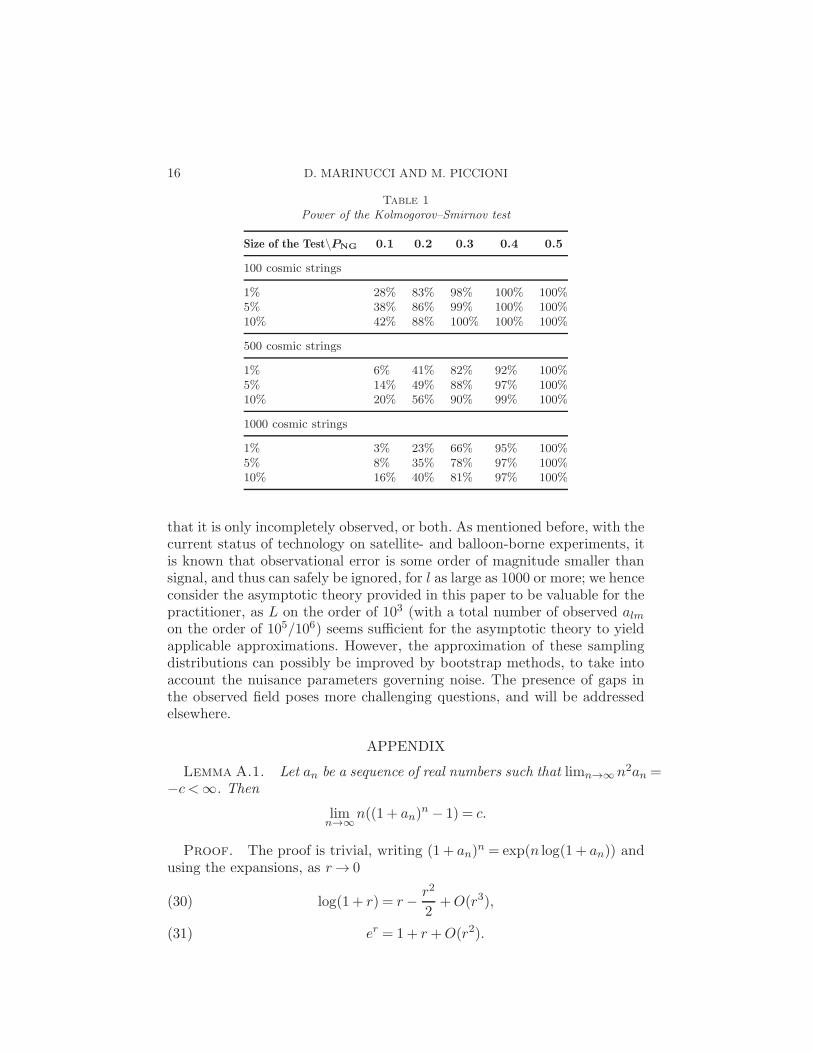
We fix L= 500, a realistic value for the MAP experiment, and we eval-uate the threshold values for sizes α = 10%, 5%, 1% by 500 Monte Carloreplications of (28): we obtain 0.947, 1.012, 1.160, respectively. We then gen-erate string maps with 100, 500 and 1000 strings, and report the rejectionfrequencies for 100 replications of model (29) (with different percentages ofnon-Gaussianity) in Table 1.
We leave several issues for future research. To increase the power of thetests, it is useful to consider empirical processes constructed on several rows[see the applied papers by Hansen, Marinucci, Natoli and Vittorio (2002)and Hansen, Marinucci and Vittorio (2003)]. As these rows are independentunder the null of Gaussianity, the extension is conceptually straightforward,although computationally burdensome. For cosmological applications, someadditional difficulties may arise in practical implementation; in particular,it may be the case that T (θ,ϕ) is subject to some measurement error, or
16 D. MARINUCCI AND M. PICCIONI
Table 1
Power of the Kolmogorov–Smirnov test
Size of the Test\PNG 0.1 0.2 0.3 0.4 0.5
100 cosmic strings
1% 28% 83% 98% 100% 100%5% 38% 86% 99% 100% 100%10% 42% 88% 100% 100% 100%
500 cosmic strings
1% 6% 41% 82% 92% 100%5% 14% 49% 88% 97% 100%10% 20% 56% 90% 99% 100%
1000 cosmic strings
1% 3% 23% 66% 95% 100%5% 8% 35% 78% 97% 100%10% 16% 40% 81% 97% 100%
that it is only incompletely observed, or both. As mentioned before, with thecurrent status of technology on satellite- and balloon-borne experiments, itis known that observational error is some order of magnitude smaller thansignal, and thus can safely be ignored, for l as large as 1000 or more; we henceconsider the asymptotic theory provided in this paper to be valuable for thepractitioner, as L on the order of 103 (with a total number of observed almon the order of 105/106) seems sufficient for the asymptotic theory to yieldapplicable approximations. However, the approximation of these samplingdistributions can possibly be improved by bootstrap methods, to take intoaccount the nuisance parameters governing noise. The presence of gaps inthe observed field poses more challenging questions, and will be addressedelsewhere.
APPENDIX
Lemma A.1. Let an be a sequence of real numbers such that limn→∞ n2an =−c <∞. Then
limn→∞
n((1 + an)n − 1) = c.
Proof. The proof is trivial, writing (1 + an)n = exp(n log(1 + an)) and
using the expansions, as r→ 0
log(1 + r) = r− r2
2+O(r3),(30)
er = 1+ r+O(r2).(31)
SPHERICAL EMPIRICAL PROCESS 17
�
The proof of the following lemma was very much shortened thanks tothe comments of one referee.
Lemma A.2. For any C > 0, as →∞,
supl−C≤x≤1
∣∣∣∣l{x−
(1 +
logx
l
)− x logx− x log2 x
2
}∣∣∣∣→ 0.
Proof. We have, uniformly in l−C ≤ x≤ 1,
l
{x−
(1 +
logx
l
)}= l
{x− exp
((l− 1) log
(1 +
logx
l
))}
= l
{x− exp
((l− 1)
(logx
l− log2 x
2l2+O
(log3 l
l3
)))}
= l
{x− exp
(logx− logx
l− log2 x
2l+O
(log3 l
l2
))}
= lx
{1− exp
(− logx
l− log2 x
2l+O
(log3 l
l2
))}
= lx
{1−
(1− logx
l− log2 x
2l+O
(log4 l
l2
))}
= x logx+x log2 x
2+O
(log4 l
l
)
= x logx+x log2 x
2+ o(1),
where we used (30) and (31). �
Lemma A.3. The marginal density of ylm = 1− exp(−lξlm) is bounded
uniformly by e2 for l≥ 2.
Proof. The marginal density of ξlm is
fξlm(t) = (l− 1)(1− t)l−21[0,1](t),
whence by the change of variable formula,
fylm(y) =l− 1
l(1− y)
(1 +
log(1− y)
l
)l−2
1[0,1−exp(−l))(y)
≤ 1
(1− y)
(1 +
log(1− y)
l
)l−2
1[0,1−exp(−l))(y).
18 D. MARINUCCI AND M. PICCIONI
Now let x= 1− y and differentiate with respect to x; we obtain
(1− 2/l)(1 + l−1 logx)l−3 − (1 + l−1 logx)l−2
x2
=−(1 + l−1 logx)l−3l−1(2 + logx)
x2,
which is equal to zero at x = e−2; the latter is easily seen to be a uniquemaximum. Hence
fYl(y)≤ e2
(1 +
log e−2
l
)l−2
≤ e2.�
Lemma A.4. As L→∞,
supα,r
|KL(α, r)− KL(α, r)|= op(1).
Proof. By the definition of KL(α, r) (14),
supα,r
|KL(α, r)− KL(α, r)| ≤1√L
L∑
l=1
1√l
l∑
m=1
1(1− l−3/2 < ylm ≤ 1);
hence, using Lemma A.3 and Markov’s inequality,
supα,r
|KL(α, r)− KL(α, r)|=Op
(L∑
l=1
√lE{1(0≤ e−lξlm < l−3/2)}
)
=Op
(1√L
L∑
l=1
1
l
)=Op
(logL√L
), as L→∞.
�
In the sequel, recall that
Zlm((α,β]) = 1(α1 < ylm ≤ β)− pl(α,β),
pl(α,β) = E1(α1 < ylm ≤ β).
Lemma A.5. As L→∞,
supα,r
|EKL(α, r)− 2√rb(α)|= o(1).
SPHERICAL EMPIRICAL PROCESS 19
Proof. By the definition of KL(α, r),
EKL(α, r)− 2√rb(α)
=1√L
[Lr]∑
l=1
[1√lbl(tl(α))
]− 2
√rb(α)
=1√L
[Lr]∑
l=1
1√l[bl(tl(α))− b(α)] + b(α)
[1√L
[Lr]∑
l=1
1√l− 2
√r
],
whose absolute value is bounded by
1√L
L∑
l=1
1√lsupα
|bl(tl(α))− b(α)|(32)
+ supα
|b(α)| supr
∣∣∣∣∣1√L
[Lr]∑
l=1
1√l− 2
√r
∣∣∣∣∣.(33)
Now for (33) we have that supα |b(α)| ≤C, whereas approximating the sumwith the integral, it is easy to see that
1√L
[Lr]∑
l=1
1√l=
1
L
[Lr]∑
l=1
1√l/L
≤∫ r
0
1√xdx= 2
√r,
and
2√r =
∫ 1/L
0
1√xdx+
∫ r
1/L
1√xdx
≤ 2√L+
1
L
[Lr]∑
l=2
1√(l− 1)/L
.
Hence
(33)≤C2√L
= o(1) as L→∞.
On the other hand, for (32) it is enough to prove that
sup0≤α≤1
|bl(tl(α))− b(α)|
≤ sup0≤α≤1−l−3/2
|bl(tl(α))− b(α)|+ sup1−l−3/2≤α≤1
|b(α)|
is o(1) as l→∞. For the second term on the right-hand side, continuity ofb(α) at α= 1 is enough. For the first, we take x= 1−α, so that we need toestablish that
liml→∞
supl−3/2≤x≤1
∣∣∣∣l{x−
(1 +
logx
l
)l−1}− 1
2x log2 x− x logx
∣∣∣∣= 0,
20 D. MARINUCCI AND M. PICCIONI
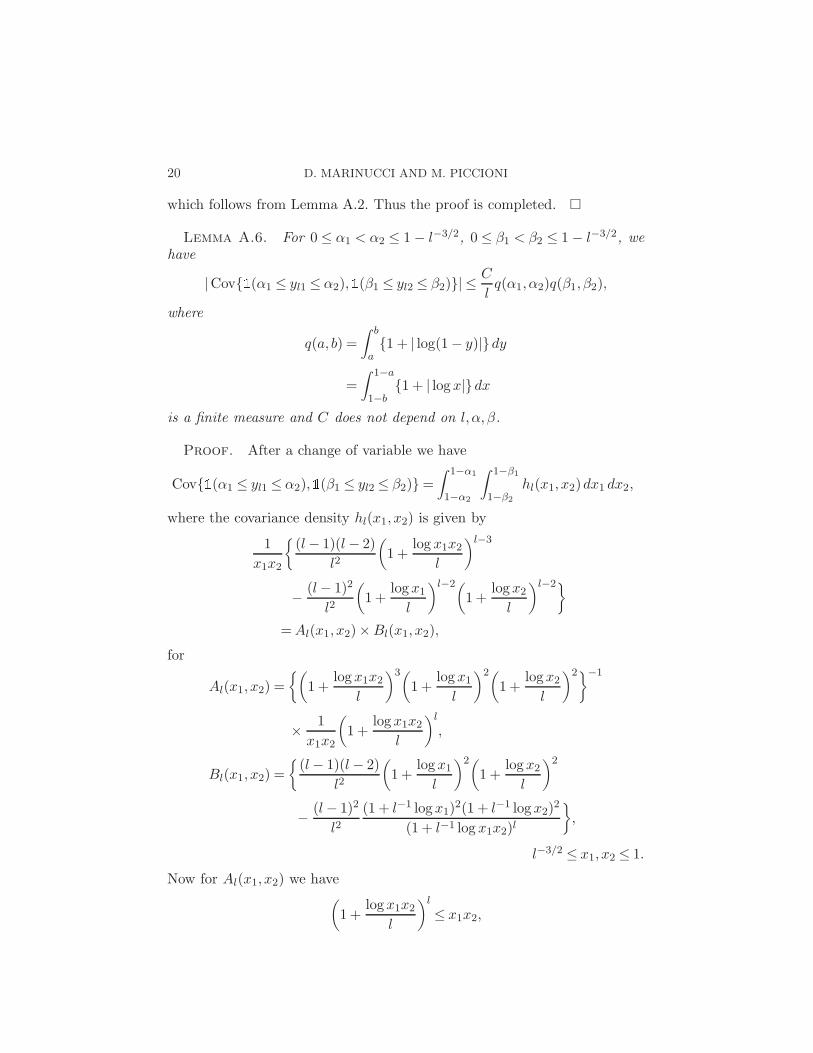
which follows from Lemma A.2. Thus the proof is completed. �
Lemma A.6. For 0 ≤ α1 < α2 ≤ 1− l−3/2, 0 ≤ β1 < β2 ≤ 1− l−3/2, we
have
|Cov{1(α1 ≤ yl1 ≤ α2),1(β1 ≤ yl2 ≤ β2)}| ≤C
lq(α1, α2)q(β1, β2),
where
q(a, b) =
∫ b
a{1 + | log(1− y)|}dy
=
∫ 1−a
1−b{1 + | logx|}dx
is a finite measure and C does not depend on l, α, β.
Proof. After a change of variable we have
Cov{1(α1 ≤ yl1 ≤ α2),1(β1 ≤ yl2 ≤ β2)}=∫ 1−α1
1−α2
∫ 1−β1
1−β2
hl(x1, x2)dx1 dx2,
where the covariance density hl(x1, x2) is given by
1
x1x2
{(l− 1)(l− 2)
l2
(1 +
logx1x2l
)l−3
− (l− 1)2
l2
(1 +
logx1l
)l−2(1 +
logx2l
)l−2}
=Al(x1, x2)×Bl(x1, x2),
for
Al(x1, x2) =
{(1 +
logx1x2l
)3(1 +
logx1l
)2(1 +
logx2l
)2}−1
× 1
x1x2
(1 +
logx1x2l
)l
,
Bl(x1, x2) =
{(l− 1)(l− 2)
l2
(1 +
logx1l
)2(1 +
logx2l
)2
− (l− 1)2
l2(1 + l−1 logx1)
2(1 + l−1 logx2)2
(1 + l−1 logx1x2)l
},
l−3/2 ≤ x1, x2 ≤ 1.
Now for Al(x1, x2) we have(1 +
logx1x2l
)l
≤ x1x2,
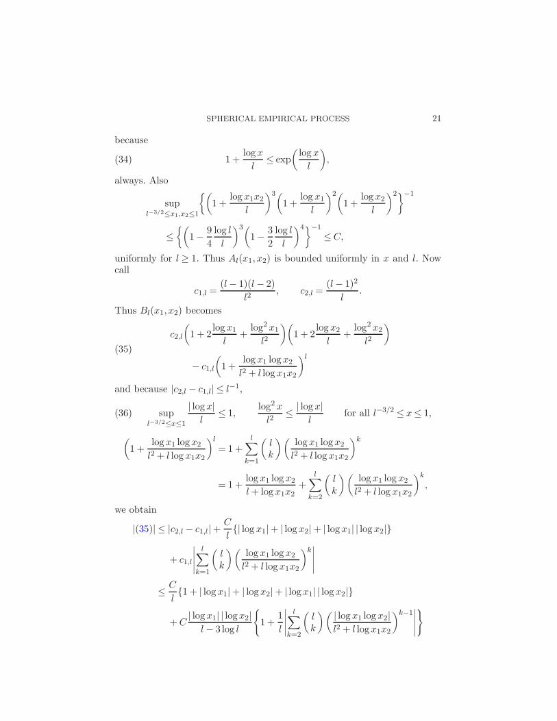
SPHERICAL EMPIRICAL PROCESS 21
because
1 +logx
l≤ exp
(logx
l
),(34)
always. Also
supl−3/2≤x1,x2≤1
{(1 +
logx1x2l
)3(1 +
logx1l
)2(1 +
logx2l
)2}−1
≤{(
1− 9
4
log l
l
)3(1− 3
2
log l
l
)4}−1
≤C,
uniformly for l ≥ 1. Thus Al(x1, x2) is bounded uniformly in x and l. Nowcall
c1,l =(l− 1)(l− 2)
l2, c2,l =
(l− 1)2
l.
Thus Bl(x1, x2) becomes
c2,l
(1 + 2
logx1l
+log2 x1l2
)(1 + 2
logx2l
+log2 x2l2
)
(35)
− c1,l
(1 +
logx1 logx2l2 + l logx1x2
)l
and because |c2,l − c1,l| ≤ l−1,
supl−3/2≤x≤1
| logx|l
≤ 1,log2 x
l2≤ | logx|
lfor all l−3/2 ≤ x≤ 1,(36)
(1 +
logx1 logx2l2 + l logx1x2
)l
= 1+l∑
k=1
(lk
)(logx1 logx2l2 + l logx1x2
)k
= 1+logx1 logx2l+ logx1x2
+l∑
k=2
(lk
)(logx1 logx2l2 + l logx1x2
)k
,
we obtain
|(35)| ≤ |c2,l − c1,l|+C
l{| logx1|+ | logx2|+ | logx1| | logx2|}
+ c1,l
∣∣∣∣∣l∑
k=1
(lk
)(logx1 logx2l2 + l logx1x2
)k∣∣∣∣∣
≤ C
l{1 + | logx1|+ | logx2|+ | logx1| | logx2|}
+C| logx1| | logx2|l− 3 log l
{1 +
1
l
∣∣∣∣∣l∑
k=2
(lk
)( | logx1 logx2|l2 + l logx1x2
)k−1∣∣∣∣∣
}
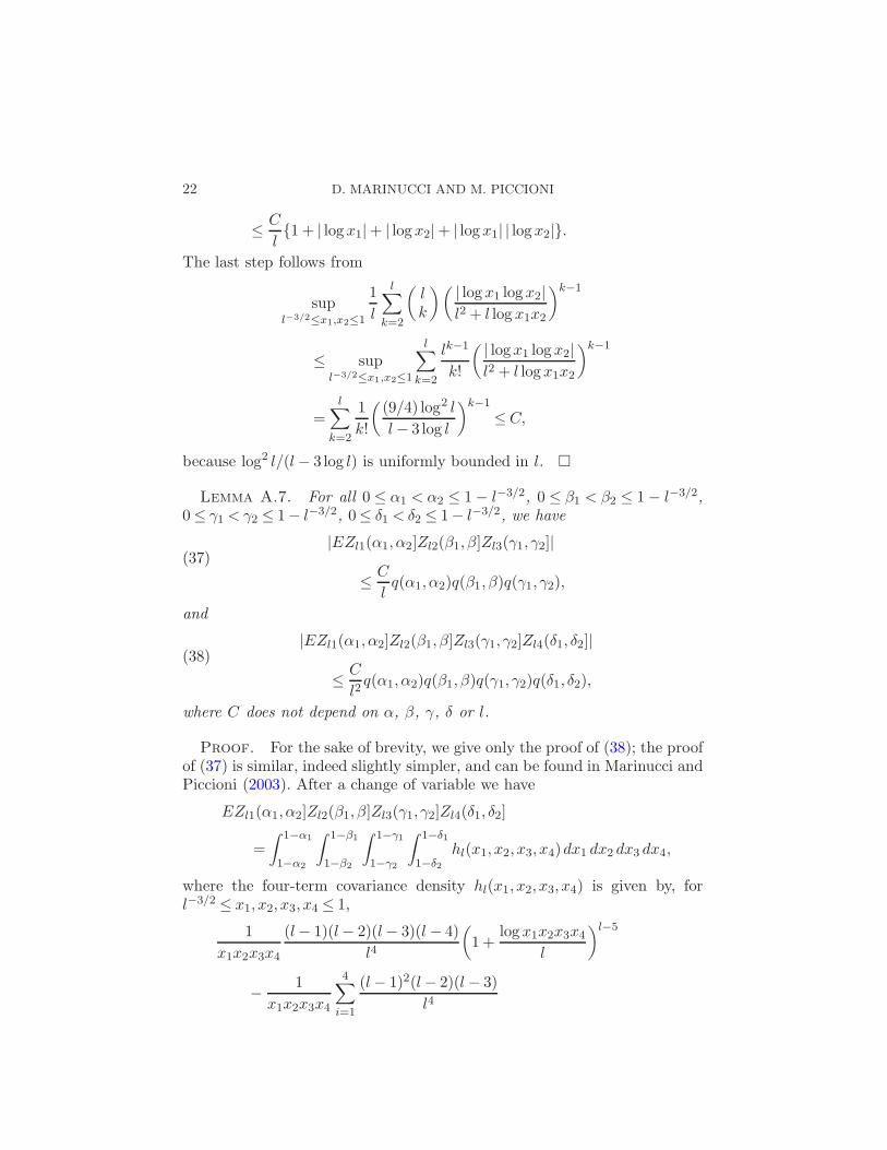
22 D. MARINUCCI AND M. PICCIONI
≤ C
l{1 + | logx1|+ | logx2|+ | logx1| | logx2|}.
The last step follows from
supl−3/2≤x1,x2≤1
1
l
l∑
k=2
(lk
)( | logx1 logx2|l2 + l logx1x2
)k−1
≤ supl−3/2≤x1,x2≤1
l∑
k=2
lk−1
k!
( | logx1 logx2|l2 + l logx1x2
)k−1
=l∑
k=2
1
k!
((9/4) log2 l
l− 3 log l
)k−1
≤C,
because log2 l/(l− 3 log l) is uniformly bounded in l. �
Lemma A.7. For all 0 ≤ α1 < α2 ≤ 1− l−3/2, 0 ≤ β1 < β2 ≤ 1− l−3/2,
0≤ γ1 < γ2 ≤ 1− l−3/2, 0≤ δ1 < δ2 ≤ 1− l−3/2, we have
|EZl1(α1, α2]Zl2(β1, β]Zl3(γ1, γ2]|(37)
≤ C
lq(α1, α2)q(β1, β)q(γ1, γ2),
and
|EZl1(α1, α2]Zl2(β1, β]Zl3(γ1, γ2]Zl4(δ1, δ2]|(38)
≤ C
l2q(α1, α2)q(β1, β)q(γ1, γ2)q(δ1, δ2),
where C does not depend on α, β, γ, δ or l.
Proof. For the sake of brevity, we give only the proof of (38); the proofof (37) is similar, indeed slightly simpler, and can be found in Marinucci andPiccioni (2003). After a change of variable we have
EZl1(α1, α2]Zl2(β1, β]Zl3(γ1, γ2]Zl4(δ1, δ2]
=
∫ 1−α1
1−α2
∫ 1−β1
1−β2
∫ 1−γ1
1−γ2
∫ 1−δ1
1−δ2hl(x1, x2, x3, x4)dx1 dx2 dx3 dx4,
where the four-term covariance density hl(x1, x2, x3, x4) is given by, forl−3/2 ≤ x1, x2, x3, x4 ≤ 1,
1
x1x2x3x4
(l− 1)(l− 2)(l− 3)(l− 4)
l4
(1 +
logx1x2x3x4l
)l−5
− 1
x1x2x3x4
4∑
i=1
(l− 1)2(l− 2)(l− 3)
l4
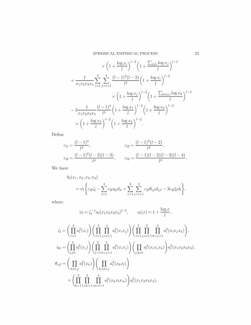
SPHERICAL EMPIRICAL PROCESS 23
×(1 +
logxil
)l−2(1 +
∑j 6=i logxj
l
)l−4
+1
x1x2x3x4
3∑
i=1
4∑
j=i+1
(l− 1)3(l− 2)
l4
(1 +
logxil
)l−2
×(1 +
logxjl
)l−2(1 +
∑k 6=j,i logxk
l
)l−4
− 31
x1x2x3x4
(l− 1)4
l4
(1 +
logx1l
)l−2(1 +
logx2l
)l−2
×(1 +
logx3l
)l−2(1 +
logx4l
)l−2
.
Define
c1l =(l− 1)4
l4, c2l =
(l− 1)3(l− 2)
l4,
c3l =(l− 1)2(l− 2)(l− 3)
l4, c4l =
(l− 1)(l− 2)(l− 3)(l− 4)
l4.
We have
hl(x1, x2, x3, x4)
= ψl
{c4lζl −
4∑
i=1
c3lηildil +3∑
i=1
4∑
j=i+1
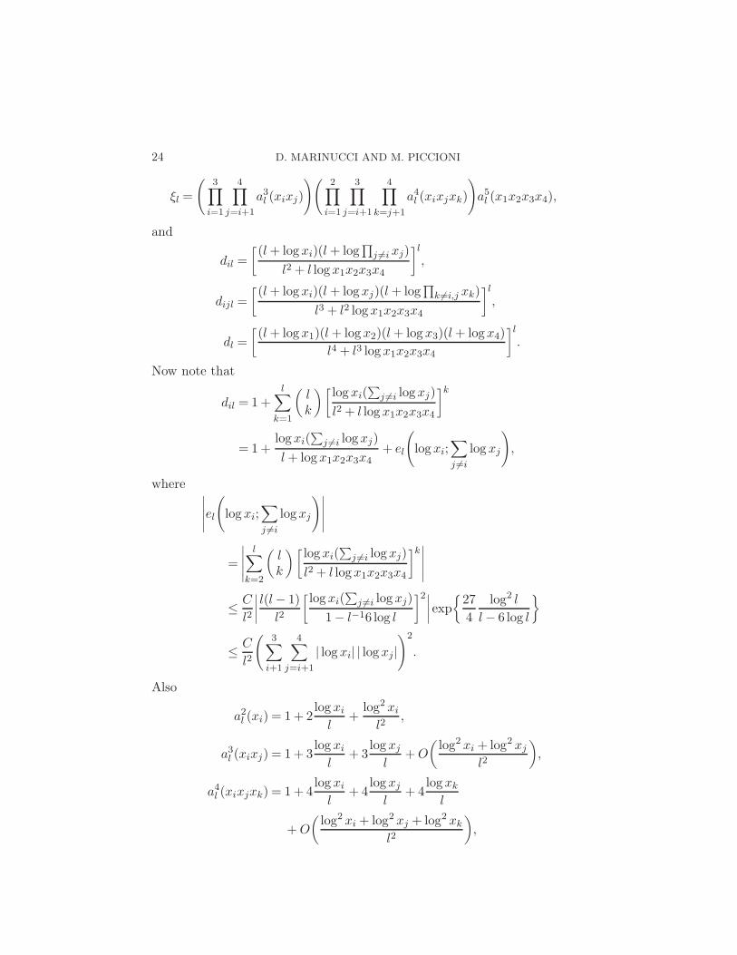
c2lθijldijl − 3c4lξldl
},
where
ψl = ζ−1l al(x1x2x3x4)
l−5, al(x) = 1 +logx
l,
ζl =
(4∏
i=1
a2l (xi)
)(3∏
i=1
4∏
j=i+1
a3l (xixj)
)(2∏
i=1
3∏
j=i+1
4∏
k=j+1
a4l (xixjxk)
),
ηil =
(4∏
j 6=i
a2l (xj)
)(3∏
j=1
4∏
k=j+1
a3l (xixj)
)( ∏
j,k 6=i
a4l (xixjxk)
)a5l (x1x2x3x4),
θijl =
( ∏
k 6=i,j
a2l (xk)
)( ∏
k,l 6=i,j
a3l (xkxl)
)
×(
2∏
k=1
3∏
l=k+1
4∏
m=l+1
a4l (xkxlxm)
)a5l (x1x2x3x4),
24 D. MARINUCCI AND M. PICCIONI
ξl =
(3∏
i=1
4∏
j=i+1
a3l (xixj)
)(2∏
i=1
3∏
j=i+1
4∏
k=j+1
a4l (xixjxk)
)a5l (x1x2x3x4),
and
dil =
[(l+ logxi)(l+ log
∏j 6=i xj)
l2 + l logx1x2x3x4
]l,
dijl =
[(l+ logxi)(l+ logxj)(l+ log
∏k 6=i,j xk)
l3 + l2 logx1x2x3x4
]l,
dl =
[(l+ logx1)(l+ logx2)(l+ logx3)(l+ logx4)
l4 + l3 logx1x2x3x4
]l.
Now note that
dil = 1+l∑
k=1
(lk
)[logxi(
∑j 6=i logxj)
l2 + l logx1x2x3x4
]k
= 1+logxi(
∑j 6=i logxj)
l+ logx1x2x3x4+ el
(logxi;
∑
j 6=i
logxj
),
where ∣∣∣∣∣el(logxi;
∑
j 6=i
logxj
)∣∣∣∣∣
=
∣∣∣∣∣l∑
k=2
(lk
)[logxi(
∑j 6=i logxj)
l2 + l logx1x2x3x4
]k∣∣∣∣∣
≤ C
l2
∣∣∣∣l(l− 1)
l2
[logxi(
∑j 6=i logxj)
1− l−16 log l
]2∣∣∣∣ exp{27
4
log2 l
l− 6 log l
}
≤ C
l2
(3∑
i+1
4∑
j=i+1
| logxi| | logxj|)2
.
Also
a2l (xi) = 1+ 2logxil
+log2 xil2
,
a3l (xixj) = 1+ 3logxil
+ 3logxjl
+O
(log2 xi + log2 xj
l2
),
a4l (xixjxk) = 1+ 4logxil
+ 4logxjl
+ 4logxkl
+O
(log2 xi + log2 xj + log2 xk
l2
),
SPHERICAL EMPIRICAL PROCESS 25
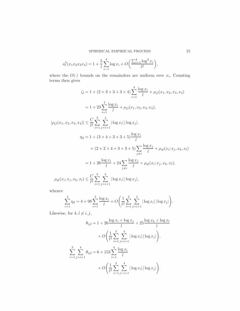
a5l (x1x2x3x4) = 1+5
l
4∑
i=1
logxi +O
(∑4i=1 log
2 xil2
),
where the O(·) bounds on the remainders are uniform over xi. Countingterms then gives
ζl = 1+ (2 + 3× 3 + 3× 4)4∑
i=1
logxil
+ ρζl(x1, x2, x3, x4)
= 1+ 234∑
i=1
logxil
+ ρζl(x1, x2, x3, x4),
|ρζl(x1, x2, x3, x4)| ≤C
l2
3∑
i=1
4∑
j=i+1
| logxi| | logxj |.
ηil = 1+ (3× 4 + 3× 3 + 5)logxil
+ (2+ 2× 4 + 3× 3 + 5)∑
j 6=i
logxjl
+ ρηl(xi;xj , xk, xl)
= 1+ 26logxil
+24∑
j 6=i
logxjl
+ ρηl(xi;xj, xk, xl),
ρηl(xi;xj, xk, xl)≤C
l2
3∑
i=1
4∑
j=i+1
| logxi| | logxj |,
whence
4∑
i=1
ηil = 4+ 984∑
i=1
logxil
+O
(1
l2
3∑
i=1
4∑
j=i+1
| logxi| | logxj|).
Likewise, for k, l 6= i, j,
θijl = 1+ 26logxi + logxj
l+ 25
logxk + logxll
+O
(1
l2
3∑
i=1
4∑
j=i+1
| logxi| | logxj|),
3∑
i=1
4∑
j=i+1
θijl = 6+ 1534∑
i=1
logxil
+O
(1
l2
3∑
i=1
4∑
j=i+1
| logxi| | logxj|).
26 D. MARINUCCI AND M. PICCIONI
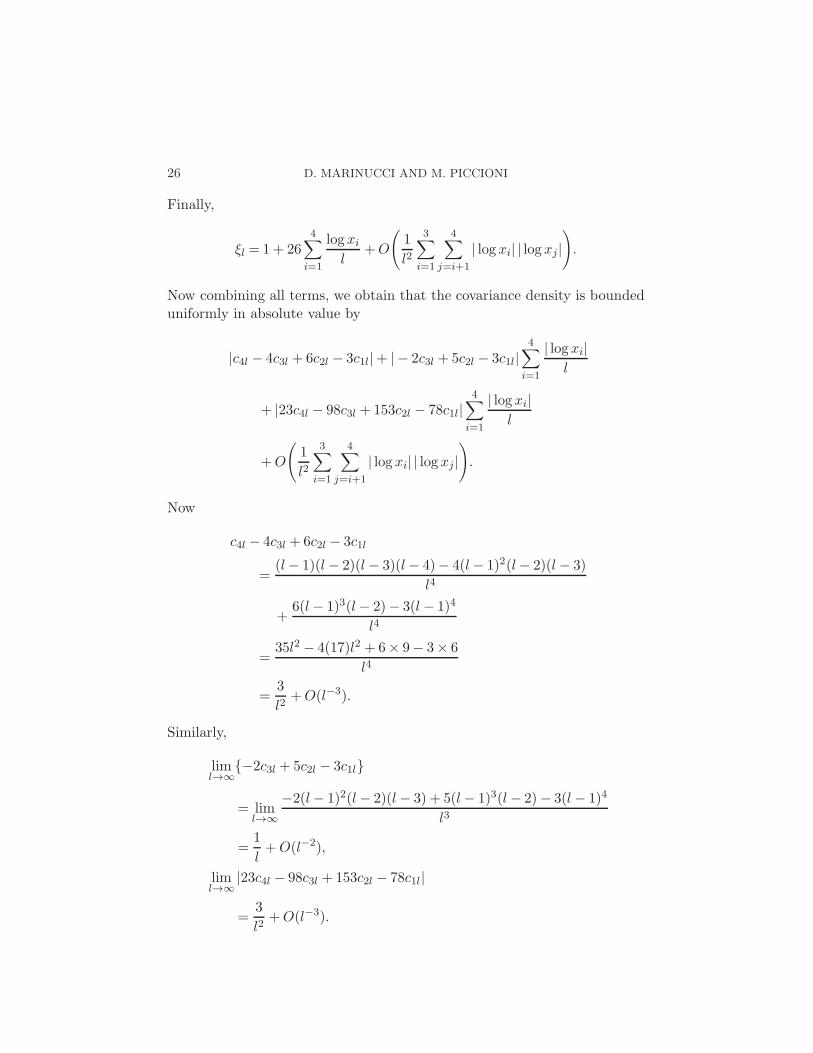
Finally,
ξl = 1+ 264∑
i=1
logxil
+O
(1
l2
3∑
i=1
4∑
j=i+1
| logxi| | logxj|).
Now combining all terms, we obtain that the covariance density is bounded
uniformly in absolute value by
|c4l − 4c3l +6c2l − 3c1l|+ | − 2c3l +5c2l − 3c1l|4∑
i=1
| logxi|l
+ |23c4l − 98c3l +153c2l − 78c1l|4∑
i=1
| logxi|l
+O
(1
l2
3∑
i=1
4∑
j=i+1
| logxi| | logxj |).
Now
c4l − 4c3l +6c2l − 3c1l
=(l− 1)(l− 2)(l− 3)(l− 4)− 4(l− 1)2(l− 2)(l− 3)
l4
+6(l− 1)3(l− 2)− 3(l− 1)4
l4
=35l2 − 4(17)l2 + 6× 9− 3× 6
l4
=3
l2+O(l−3).
Similarly,
liml→∞
{−2c3l +5c2l − 3c1l}
= liml→∞
−2(l− 1)2(l− 2)(l− 3) + 5(l− 1)3(l− 2)− 3(l− 1)4
l3
=1
l+O(l−2),
liml→∞
|23c4l − 98c3l +153c2l − 78c1l|
=3
l2+O(l−3).
SPHERICAL EMPIRICAL PROCESS 27
It can thus be concluded that the four-term covariance density is boundeduniformly by
hl(x1, x2, x3, x4)≤C
l2
{1 +
4∑
i=1
| logxi|+3∑
i=1
4∑
j=i+1
| logxi| | logxj|}
≤ C
l2
4∏
i=1
{1 +
4∑
i=1
| logxi|},
and thus the proof is completed. �
Acknowledgments. We are very grateful to two anonymous referees whosecomments greatly improved the presentation of this paper. We are also grate-ful to F. Hansen, P. Natoli and N. Vittorio, from the Cosmology Group atthe University of Rome “Tor Vergata,” for bringing this problem to our at-tention and for many fruitful discussions. Finally, we thank F. Hansen forcarrying out the simulations in Section 4.
REFERENCES
Bickel, P. J. and Wichura, M. J. (1971). Convergence criteria for multiparame-ter stochastic processes and some applications. Ann. Math. Statist. 42 1656–1670.MR383482
Dore, O., Colombi, S. and Bouchet, F. R. (2003). Probing cosmic microwave back-ground non-Gaussianity using local curvature. Monthly Notices R. Astronom. Soc. 344
905–916. Available at arxiv.org as astro-ph/0202135.Dudley, R. M. (1999). Uniform Central Limit Theorems. Cambridge Univ. Press.
MR1720712Hannan, E. J. (1970). Multiple Time Series. Wiley, New York. MR279952Hansen, F. K., Marinucci, D., Natoli, P. and Vittorio, N. (2002). Testing for non-
Gaussianity of the cosmic microwave background in harmonic space: An empirical pro-cess approach. Phys. Rev. D 66 63006/1-14. Available at arxiv.org as astro-ph/0206501.
Hansen, F. K., Marinucci, D. and Vittorio, N. (2003). Extended empirical processtest for non-Gaussianity in the CMB, with an application to non-Gaussian inflationarymodels. Phys. Rev. D 67 123004/1-7. Available at arxiv.org as astro-ph/0302202.
Johnson, N. L. and Kotz, S. J. (1972). Distributions in Statistics: Continuous Multi-
variate Distributions. Wiley, New York. MR418337Komatsu, E. and Spergel, D. N. (2001). Acoustic signatures in the primary mi-
crowave background bispectrum. Phys. Rev. D 63 63002/1-13. Available at arxiv.orgas astro-ph/0005036.
Leonenko, N. N. (1999). Limit Theorems for Random Fields with Singular Spectrum.Kluwer, Dordrecht. MR1687092
Liboff, R. L. (1998). Introductory Quantum Mechanics, 3rd ed. Addison-Wesley, Reading,MA.
Marinucci, D. and Piccioni, M. (2003). The empirical process on Gaussian sphericalharmonics. Working Paper n. 7, Dip. Matematica, Universita di Roma “La Sapienza.”
Miller, C. J., Nichol, R. C., Genovese, C. and Wasserman, L. (2002). A nonpara-metric analysis of the cosmic microwave background power spectrum. Astrophys. J. 565
L67–L70. Available at arxiv.org as astro-ph/0112049.
28 D. MARINUCCI AND M. PICCIONI
Novikov, D., Schmalzing, J. and Mukhanov, V. F. (2000). On non-Gaussianity inthe cosmic microwave background. Astronomy and Astrophysics 364 17–25. Availableat arxiv.org as astro-ph/0006097.
Peacock, J. A. (1999). Cosmological Physics. Cambridge Univ. Press.Peebles, P. J. E. (1993). Principles of Physical Cosmology. Princeton Univ. Press.
MR1216520Phillips, N. G. and Kogut, A. (2001). Statistical power, the bispectrum and the search
for non-Gaussianity in the cosmic microwave background anisotropy. Astrophys. J. 548
540–549. Available at arxiv.org as astro-ph/0010333.Shorack, G. (1972). Convergence of quantile and spacings processes with applications.
Ann. Math. Statist. 43 1400–1411. MR359133Shorack, G. and Wellner, J. (1986). Empirical Processes with Applications to Statis-
tics. Wiley, New York. MR838963van der Vaart, A. andWellner, J. (1996). Weak Convergence and Empirical Processes.
Springer, New York. MR1385671Varshalovich, D. A., Moskalev, A. N. and Khersonskii, V. K. (1988). Quantum
Theory of Angular Momentum. World Scientific, Singapore. MR1022665Wasserman, L., Miller, C., Nichol, B., Genovese, C., Jang, W., Connolly, A.,
Moore, A., Schneider, J. and the PICA Group (2001). Nonparametric inferencein astrophysics. Preprint. Available at arxiv.org as astro-ph/0112050.
Winitzki, S. and Wu, J. H. P. (2000). Inter-scale correlations as measures of CMBGaussianity. Preprint. Available at arxiv.org as astro-ph/0007213.
Wong, E. (1971). Stochastic Processes in Information and Dynamical Systems. McGraw-Hill, New York.
Dipartimento di Matematica
Universita di Roma “Tor Vergata”
via della Ricerca Scientifica 1
00133 Roma
Italy
e-mail: [email protected]
Dipartimento di Matematica
Universita di Roma “La Sapienza”
Piazzale Aldo Moro 2
00185 Roma
Italy
e-mail: [email protected]