The Emperor has no Clothes:Limits to Risk Modelling

Jon Danıelsson∗

Financial Markets GroupLondon School of Economics

www.RiskResearch.org

June 2000

Abstract

This paper considers the properties of risk measures, primarily Value–at–Risk(VaR), from both internal and external (regulatory) points of view. It is arguedthat since market data is endogenous to market behavior, statistical analysismade in times of stability does not provide much guidance in times of crisis. Inan extensive survey across data classes and risk models, the empirical propertiesof current risk forecasting models are found to be lacking in robustness whilebeing excessively volatile. For regulatory use, the VaR measure is lacking inthe ability to fulfill its intended task, it gives misleading information about risk,and in some cases may actually increase both idiosyncratic and systemic risk.Finally, it is hypothesized that risk modelling is not an appropriate foundationfor regulatory design, and alternative mechanisms are discussed.

∗I have benefited from comments by Richard Payne, Casper de Vries, Charles Goodhart, KevinJames, and Bob Nobay; the mistakes and analysis is of course my responsibility alone. For cor-respondence j.danielsson@lse.ac.uk. My papers can be downloaded from www.RiskResearch.org orfmg.lse.ac.uk/˜jond.

1 Introduction

Recent years have witnessed an enormous growth in financial risk modelling bothfor regulatory and internal risk management purposes. There are many reasonsfor this; stronger perception of the importance of risk management, deregulationenabling more risk taking, and technical advances encouraging both risk takingand facilitating the estimation and forecasting of risk. This impact has been feltin regulatory design: market risk regulations are now model based, and we seeincreasing clamoring for regulatory credit risk modelling. The motivations formarket risk modelling are obvious. The data is widely available, a large numberof models analyzing financial data exist, rapid advances in computer technologyenable the estimation of the most complicated models, and the ever–increasingsupply of well educated graduates, all led to a sense of “can do” within thetechnical modelling community. Empirical modelling has been of enormous usein applications such as derivatives pricing and risk management, and is beingapplied successfully to the new fields of credit and operational risk.

There is however precious little evidence that risk modelling actually works.Has risk management delivered? We don’t know for sure, and probably neverwill. If regulatory risk management fulfills its objectives, we will not observeany systemic failures, so only the absence of crisis can prove the system works.There is however an increasing body of evidence that inherent limitations in riskmodelling technology, coupled with imperfect regulatory design, is more like aplacebo rather than the scientifically proven preventer of crashes it is sometimesmade out to be. Below I survey some of this evidence; the general inaccuracy andlimitations of current risk models, the impact of (externally imposed uniform)risk constraints on firm behavior, the relevance of statistical risk measures, andthe feedback between market data, risk models, and the beliefs of market partic-ipants. I finally relate this evidence to the current debate on regulatory designwhere I argue against the notion of model based regulations, be it for market,credit, or operational risk.

An explicit assumption in most risk models is that market price data follows astochastic process which only depends on past observations of itself and othermarket data, not on outside information. While this assumption is made tofacilitate modelling1, it relies on the hypothesis that there are so many marketparticipants, and they are so different that in the aggregate their actions areessentially random and can not influence the market. This implies that therole of the risk forecaster is akin to a meteorologists job, who can forecast theweather, but not influence it. This approach to modelling has a number ofshortcomings from the point of view of financial markets. If risk measurementsinfluence people’s behavior, it is inappropriate to assume market prices followan independent stochastic process. This becomes especially relevant in times

1Incorporating outside information in statistical risk models is very hard

2

of crisis when market participants hedge related risks leading to the executionof similar trading strategies. The basic statistical properties of market dataare not the same in crisis as they are during stable periods; therefore, mostrisk models provide very little guidance during crisis periods. In other words,the risk properties of market data change with observation. If, in addition,identical external regulatory risk constraints are imposed, regulatory demandsmay perversely lead to the amplification of the crisis by reducing liquidity. Thereis some evidence that this happened during the 1998 crisis. Indeed, the past 3years have not only been the most volatile in the 2nd half of the 20th centurybut also the era of intensive risk modelling.

In order to forecast risk, it is necessary to assume a model which in turn is esti-mated with market price data. This requires a number of assumptions regardingboth model design and the statistical properties of the data. It is not possible tocreate a perfect risk model, and the risk forecaster needs to weigh the pros andcons of the various models and data choices to create what inevitably can onlybe an imperfect model. I present results from an extensive survey of model riskforecast properties, employing a representative cross–section of data and modelsacross various estimation horizons and risk levels. The results are less than en-couraging. All the models have serious problems with lack of robustness and highrisk volatility, implying that unless a risk model is chosen with considerable skilland care, the model outcomes will be as accurate as predictions of the outcomesof a roulette wheel. Off–the–shelf models can not be recommended.

Current market risk regulations are based on the 99% Value–at–Risk (VaR) mea-sure obtained from a risk model. The VaR number can, under some assumptions,provide an adequate representation of risk, however such assumptions are oftenunrealistic, and result in the misrepresentation of risk. There are (at least) fourproblems with the regulatory VaR measure. First, it does not indicate potentiallosses, and as a result is flawed, even on its own terms. Second, it is not a co-herent measure of risk. Third, its dependence on a single quantile of the profitand loss distribution implies it is easy to manipulate reported VaR with speciallycrafted trading strategies. Finally, it is only concerned with the 99% loss level,or a loss which happens 2.5 times a year, implying that VaR violations have verylittle relevance to the probability of bankruptcy, financial crashes, or systemicfailures.

The role of risk modelling in regulatory design is hotly debated. I argue that theinherent flaws in risk modelling imply that neither model based risk regulationsnor the risk weighing of capital can be recommended. If financial regulations aredeemed necessary, alternative approaches such as state contingent capital levelsand/or cross–insurance systems are needed.

3

2 Risk Modelling and Endogenous Response

The fundamental assumption in most statistical risk modelling is that the basicstatistical properties of financial data during stable periods remain (almost) thesame as during crisis. The functional form of risk models is usually not updatedfrequently, and model parameters get updated slowly.2 This implies that riskmodels can not work well in crisis. The presumed inability of risk models towork as advertised has not gone unnoticed by commentators and the popularpress;

“Financial firms employed the best and brightest geeks to quantify anddiversify their risks. But they have all – commercial banks, investmentbanks and hedge funds – been mauled by the financial crisis. Now theyand the worlds regulators are trying to find out what went wrong andto stop it happening again. ... The boss of one big firm calls super–sophisticated risk managers ‘high–IQ morons’ ”The Economist, November 18, 1998, pp. 140–145.

There is a grain of truth in this quote: Statistical financial models do break downin crisis. This happens because the statistical properties of data during crisis isdifferent than the statistical properties in stable times. Hence, a model createdin normal times may not be of much guidance in times of crisis. Morris and Shin(1999) suggest that most statistical risk modelling is based on a fundamentalmisunderstanding of the properties of risk. They suggest that (most) risk mod-elling is based on the incorrect assumption of a single person (the risk manager)solving decision problems with a natural process (risk). The risk manager inessence treats financial risk like the weather, where the risk manager assumes arole akin to a meteorologist. We can forecasts the weather but can not changeit, hence risk management is like a “game against nature”. Fundamental tothis is the assumption that markets are affected by a very large number of het-erogeneous market participants, where in the aggregate their actions become arandomized process, and no individual market participant can move the markets.This is a relatively innocuous assumption during stable periods, or in all peri-ods if risk modelling is not in widespread use. However, the statistical processof risk is different from the statistical process of the weather in one importantsense: forecasting the weather does not (yet) change the statistical properties ofthe weather, but forecasting risk does change the nature of risk. In fact, this isrelated to Goodharts Law:

Law 1 (Goodhart (1974)) Any statistical relationship will break down whenused for policy purposes.

2Models, such as GARCH, do of course pick up volatility shocks, but if the parameterization andestimation horizon remain the same, the basic stochastic process is the same, and the model has thesame steady state volatility, which is only updated very slowly.

4

We can state a corollary to this

Corollary 1 A risk model breaks down when used for its intended purpose.

Current risk modelling practices are similar to pre–rational expectations Key-nesian economics in that risk is modelled with behavioral equations that areinvariant under observation. However, just as the economic crisis of the 1970’sillustrated the folly of the old style Keynesian models, so have events in finan-cial history demonstrated the limitations of risk models. Two examples serve toillustrate this. The Russia crisis of 1998 and the stock market crash of 1987.

Consider events during the 1998 Russia crisis. (See e.g. Dunbar (1999)). At thetime risk had been modelled with relatively stable financial data. In Figure 3on page 26 we see that the world had been in a low volatility state for thepreceding half a decade, volatility had somewhat picked up during the Asiancrisis of 1997, but those volatility shocks were mostly confined to the Far East,and were leveling off in any case. In mid year 1998 most financial institutionsemployed similar risk model techniques and often similar risk constrains becauseof regulatory considerations. When the crisis hit, volatility for some assets wentfrom 16 to 40, causing a breach in many risk limits. The response was decidedlyone–sided, with a general flight from volatile to stable assets. This of courseamplified price movements and led to a sharp decrease in liquidity. In otherwords, the presence of VaR based risk limits led to the execution of similartrading strategies, escalating the crisis.

This is indeed similar to events surrounding a previous crisis, the 1987 crash whena method called portfolio insurance was very much in vogue. (See e.g. Jacobs(1999)). An integral component in portfolio insurance is that complicated hedg-ing strategies with futures contracts are used to dynamically replicate options inorder to contain downside risk. These dynamic trading strategies worked well inthe stable pre–crisis periods since they depended on the presence of functioningfutures markets. However, one characteristic of the ’87 crash was that the futuresmarkets ceased to function properly because the institutions who used portfolioinsurance were trying to execute identical trading strategies, which only servedto escalate the crisis.

If every financial institution has its own trading strategy, no individual techniquecan lead to liquidity crisis. However, each institution’s behavior does move themarket, implying that the distribution of profit and loss is endogenous to thebanks decision–making process. In other words, risk is not the separate stochas-tic variable assumed by most risk models, instead, risk modelling affects thedistribution of risk. A risk model is a model of the aggregate actions of marketparticipants, and if many of these market participants need to execute the sametrading strategies during crisis, they will change the distributional properties ofrisk. As a result, the distribution of risk is different during crisis than in otherperiods, and risk modelling is not only useless but may exasperate the crisis, byleading to large price swings and lack of liquidity.

5

The role played by regulation during these scenarios is complex. It is rationalfor most banks to reduce exposure in the event of a risk shock, independent ofany regulatory requirements, and if banks have similar incentives and employsimilar risk models, that alone can lead to a snowball effect in trading strategiesduring crisis. Indeed this is what happened during the 1987 crisis when regula-tion played no direct role. However, if regulation restricts the banks scope forpursuing individually optimal strategies, causing banks to act in a more uniformmanner during crisis it may lead to an escalation of the crisis. Whether thisactually happens is yet unknown. In the current regulatory environment, thebanks themselves model risk, hence risk models are individual to the bank andas a results not all institutions follow the same risk control trading strategy.Hence, regulation may not be the straight–jacket one might think. However, theburden of proof is on the regulators to demonstrate that the regulations do notescalate the crisis. They have not yet done so.

The analysis presented here does not imply that risk modelling is inherentlypointless. Internally, banks do benefit from hedging as demonstrated by e.g.Froot, Scharfstein, and Stein (1993), and risk models are reliable in stable pe-riods, especially in dealing with idiosyncratic shocks. However, even though(most) current risk models are useless during crisis, this is only a reflection ofthe current state of risk technology. Risk models grounded in the microeconomictheory of financial crisis, have considerable promise.

3 Empirical Properties of Risk Models

Risk forecasting depends on a statistical model and historical market price data.The modeller makes a number of assumptions about the statistical propertiesof the data, and from that specifies the actual model. This model will alwaysbe based on objective observations and subjective opinions, and therefore thequality of the model depends crucially on the modeller’s skill. As a result, it isnot possible to create a perfect model. Each model has flaws, where the modellerweighs the pros and cons of each technique and data set, juggling issues like thechoice of the actual econometric model, the length of the estimation horizon,the forecast horizon, and the significance level of the forecasts. In fact, dueto these limitations, the resulting model is endogenous to its intended use. Twodifferent users, who have different preferences but identical positions and views ofwhat constitutes risk, require different risk forecasts. This happens because riskmodelling is conditional on the user’s loss functions. The weighing of the pros andcons is different for different users, resulting in different risk models and hencedifferent risk forecasts, even for identical positions. In order to address some ofthese issues I refer below to results from a survey I made (Danıelsson 2000) ofthe forecast properties of various models and data sets.

The data is a sample from the major asset classes, equities, bonds, foreign ex-

6

change, and commodities. Each data set consists of daily observations and spansat least fifteen years. The discussion below is based on forecasts of day–by–dayValue–at–Risk during the 1990s (2500 forecasts per dataset on average) The risklevel is mostly the regulatory 99% but I also consider lower and higher risk lev-els. The survey was done with a single asset return. While a portfolio approachwould be more appropriate, this raises a number of issues which I thought bestavoided. As such, my survey only presents a best case scenario, most favorableto risk models.

A large number of risk models exist and it is not possible to examine each andevery one. However, most models are closely related to each other, and by usinga carefully selected subsample I am confident that I cover the basic properties ofmost models in use. The models studied are:

• Conditional volatility models (normal3 and student–t GARCH)

• Unconditional models (historical simulation (HS) and extreme value theory(EVT))

(More details on the survey can be found in Appendix A.)

The risk modeller is faced with many challenges, some of the most importantare:

• Robustness of risk forecasts (Section 3.1)

• Volatility of risk forecasts (Section 3.2 on page 9)

• Determination of the appropriate measuring horizon (Section 3.3 on page 10)

• Determination of the holding period (Section 3.4 on page 11)

• Underestimation of downside risk due to asymmetries in correlation struc-tures (Section 3.5 on page 13)

3.1 Robustness of Risk Forecasts

For a risk model to be considered reliable, it should provide accurate risk forecastsacross different assets, time horizons, and risk levels within the same asset class.The robustness of risk models has been extensively documented, and there is notmuch reason to report detailed analysis here, my results correspond broadly tothose from prior studies. I use violation ratios4 to measure the accuracy of riskforecasts. If the violation ratio is larger than 1, the model is underforecastingrisk (it is thin tailed relative to the data), and if the violation ratio is lowerthan 1, the model is overforecasting risk (the model is thick tailed relative to the

3The RiskMetricsTM model is a restricted normal GARCH model (IGARCH) and hence its per-formance can only be worse than for the normal GARCH.

4The realized number of VaR violations over expected number of violations. By violation I meanthat realized loss was larger than the VaR forecast

7

data). Violation ratios are the most common method for ranking models, sincethey directly address the issue of forecast accuracy. The risk level used is theregulatory 99%, see Table 1 on page 24.

An ideal model has violation ratios close to 1 across asset classes and significancelevels. While what constitutes “close to 1” is subjective, the range of 0.8 to 1.2is a useful compromise. Based on this criteria, the results are depressing. Forexample, the normal GARCH model produces violation ratios ranging from 0.37to 2.18, and even for the same data set, e.g. S&P–500, the violation ratiosrange from 0.91 to 1.46. The other estimation methods have similar problemsbut not on the same scale. Every method overestimates the bond risk, andunderestimates the risk in Microsoft stock. The normal GARCH model (andby extension RiskMetricsTM) has the overall worst performance, the results forthe other models are mixed. Danıelsson (2000) reports that a similar pictureemerges from all considered risk levels, but the ranking among models changes.At the 95% risk level, the normal GARCH model performs generally best, whileat 99.9% EVT is best.

It is also interesting to consider the importance of the estimation horizon. Con-ventional wisdom seems to be that short horizons are preferred, say one year or250 days. This is indeed a regulatory recommendation in some cases. It is how-ever not supported by my results. For example, for oil prices and the Student–tGARCH model, the violation ratio is 1.38 when the model is estimated with300 days, and only 1.04 when the model is estimated with 2,000 days. Similarresults have been obtained in some other cases. The reason has to do with thefact that a conditional volatility reverts to the steady state volatility, which isdependent on the estimation horizon. If the estimation horizon is too short, themodel steady state volatility reflects past high/low volatility states which areless relevant than the long run average.

These results show that no model is a clear winner. The forecasts, cover a verywide range, and the lack of robustness is disconcerting. Furthermore, the estima-tion horizon has considerable impact on the forecast accuracy. One conclusionis that none of these models can be recommended, but since these models formthe basis of almost every other model, this recommendation is too strong. Myapproach here is to use off-the–shelf models. A skilled risk manager consideringspecific situations is able to specify much more accurate models. This is indeedthe situation internally in many banks. For reporting purposes, where the VaRnumber is an aggregate of all the banks risky positions, the use of an accuratespecially designed model is much harder and off–the–shelf models are more likelyto be used. This coupled with ad hoc aggregation methods for risk across op-erations, and the lack of coherence in VaR, can only have an adverse effect onmodel accuracy.

8

3.2 Risk Volatility

Fluctuations in risk forecasts have serious implications for the usefulness of a riskmodel; however, risk forecast fluctuations have not been well documented. Thereason for this is unclear, but the importance of this issue is real. If a financialinstitution has a choice between two risk models both of which forecast equallywell, but one model produces much less volatile forecasts, it will be chosen. Andif risk forecasts are judged to be excessively volatile, it may hinder the use ofrisk forecasting within a bank. If a VaR number routinely changes by a factorof 50% from one day to the next, and factor 2 changes are occasionally realized,it may be hard to sell risk modelling within the firm. Traders are likely to beunhappy with widely fluctuating risk limits, and management does not like tochange market risk capital levels too often. This is due to many reasons, oneof them phantom price volatility. Furthermore Andersen and Bollerslev (1998)argue that there is an built–in upper limit on the quality of volatility forecasts(around 47%).

In my survey I use two measures of fluctuations in risk forecasts;

• The volatility of the VaR, i.e. the standard deviation of VaR forecasts overthe sample period

• The VaR forecast range, i.e. the maximum and minimum VaR forecast overthe sample period

Both measures are necessary. The VaR volatility addresses the issue of day–to–day fluctuations in risk limits, while the VaR range demonstrates the worst–casescenarios.

A representative sample of the results using the S&P–500 index is presentedbelow in Table 2 on page 25. Consider e.g. the regulatory 99% level and the300 day estimation horizon. The return volatility is 0.9%, and the volatilityof the VaR estimates is 0.7% It is almost like we need a risk model to accessthe risk in the risk forecasts! The largest drop in returns is -7.1% (in 2527observations), while the lowest normal GARCH model forecast is -7.5% at the99% level or an event once every 100 days. With longer estimation horizons boththe volatility and the range decrease, suggesting that longer estimation horizonsare preferred. The same results are obtained from the other data sets. Anotherinteresting result is that the least volatile methods are historical simulation (HS)and extreme value theory (EVT). The reason is that conditional volatility modelsare based on a combination of long estimation horizons (more than 250 days)along with very short run VaR updating horizons (perhaps five days). In contrast,the HS and EVT methods are unconditional and as a result produce less volatilerisk forecasts. Note that a hybrid conditional volatility and EVT method, such asthe methods proposed by McNeil and Frey (1999) produce VaR forecasts whichare necessarily more volatile than the condition volatility methods.

9

The contrast between GARCH and EVT volatility can be seen in Figure 4 onpage 27 which shows Hang Seng index returns during the last quarter of 1997. Setin the middle of the Asian crisis, the Hang Seng index is very volatile, with thelargest one day drop of more than 15%. Both models have an excessive amount ofviolations, but while the EVT forecast is relatively stable throughout the quarter,the GARCH forecast is very volatile. The lowest GARCH VaR is 19%, and themodel takes more than a month to stabilize after the main crash. In addition,the main contributor to the GARCH VaR volatility is the positive return of18% following the main crash. Since conditional volatility models like GARCHhave a symmetric response to market movements, a positive and negative marketmovement has the same impact on the VaR.

Because the Value–at–Risk numbers are quantiles of the profit and loss distribu-tion it is not surprising that they are volatile. However, I find them surprisinglyvolatile. It is not uncommon for VaR numbers to double from one day to thenext, and then revert back. If VaR limits were strictly adhered to, the costsof portfolio rebalancing would be large. This has not gone unnoticed by thefinancial industry and regulators. Anecdotal evidence indicates that many firmsemploy ad hoc procedures to smooth risk forecasts. For example, a bank mightonly update its covariance matrix every three months, or treat risk forecastsfrom conditional volatility models as an ad hoc upper limit for daily risk lim-its. Alternatively, covariance matrices are sometimes smoothed over time usingnon–optimal procedures. If Value–at–Risk is used to set risk limits for a tradingdesk, strict adherence to a VaR limit which changes by a factor of two from oneday to the next is indeed costly. The same applies to portfolio managers whoneed to follow their mandate, but would rather not rebalance their portfoliostoo often. In addition, since regulatory VaR is used to determine market riskcapital, a volatile VaR leads to costly fluctuations in capital if the financial insti-tution keeps its capital at the minimum level predicted by the model. This mayturn cause lack of confidence in risk models and hinder their adoption within afirm. Anecdotal evidence indicates that (some) regulators consider bank capitalas a constant to be allocated to the three categories of risk, market, credit, andoperational, and not the widely fluctuating quantity predicted by the models.

3.3 Model Estimation Horizon

The estimation of a risk model depends on sufficiently long historical data seriesbeing available. The regulatory suggestion is (at least) 250 days, and anecdotalevidence indicates that short estimation horizons are very much preferred. Thismust be based on one of two assumptions;

• Older data is not available, or is irrelevant due to structural breaks

• Long run risk dynamics are so complicated that they can’t be modelled

10

While the first assumption is true in special cases, e.g. immediately after anew instrument is introduced such as the Euro, and in emerging markets, ingeneral, it is not correct. The second assumption is partially correct: long runrisk dynamics are complicated and often impossible to model explicitly; however,long run patterns can be incorporated, it just depends on the model.

Long run risk dynamics are not a well understood and documented phenomena,but it is easy to demonstrate the existence of long cycles in volatility. ConsiderFigure 3 on page 26 which demonstrates changes in average daily volatility forthe second half of the 20th century. Daily volatility ranges from 0.5% to almost2% in a span of few years. The 1990s demonstrate the well–known U–shapedpattern in volatility.

Observing these patterns in volatility is one thing, modelling them is another.Although existing risk models do not yet incorporate this type of volatility dy-namics, conceivably this it possible. Most conditional volatility models, e.g.GARCH, incorporate both long run dynamics (through parameter estimates)and very short–term dynamics (perhaps less than one week). Long memoryvolatility models may provide the answers; however, their risk forecasting prop-erties are still largely unexplored.

The empirical results presented in Table 1 on page 24 and Table 2 on page 25 showthat shorter estimation horizons do not appear to contribute to more accurateforecasting, but longer estimation horizons do lead to lower risk volatility. Forthat reason alone longer estimation horizons are preferred.

3.4 Holding Periods and Loss Horizons

Regulatory Value–at–Risk requires the reporting of VaR for a 10 day holdingperiod. This is motivated by a fear of liquidity crisis where a financial institutionmight not be able to liquidate its holdings for 10 days straight. While this maybe theoretically relevant, two practical issues arise;

• The contradiction in requiring the reporting of a 10 day 99% Value–at–Risk, i.e. a two week event which happens 25 times per decade, in order tocatch a potential loss due to a liquidity crisis which is unlikely to happeneven once a decade. Hence the probability and problem are mismatched.

• There are only two different methods of doing 10 day Value–at–Risk inpractice:

– Use non–overlapping5 10 day returns to produce the 10 day Value–at–Risk forecast

– Use a scaling law to convert one day VaRs to 10 day VaRs (recom-mended by the Basel Committee on Banking Supervision (1996))

5Overlapping returns cannot be used for obvious reasons

11

Both of these methods are problematic

If 10 day returns are used to produce the Value–at–Risk number, the data re-quirements obviously also increase by a factor of 10. For example, if 250 days(one year) are used to produce a daily Value–at–Risk number, ten years of dataare required to produce a 10 day Value–at–Risk number with the same statisticalaccuracy. If however 250 days are used to produce 10 day Value–at–Risk num-bers, as sometimes is recommended, only 25 observations are available for thecalculation of something which happens in one observation out of every hundred,clearly an impossible task. Indeed, at least 3,000 days are required to directlyestimate a 99% 10 day VaR, without using a scaling law.

To bypass this problem most users tend to follow the recommendation in theBasel regulations (Basel Committee on Banking Supervision 1996) and use theso–called ‘square–root–of–time’ rule, where a one day VaR number is multipliedby the square root of 10 to get a 10 day VaR number. However, this depends onsurprisingly strong distribution assumptions, i.e. that returns are normally iid:

• Returns are normally distributed

• Volatility is independent over time

• The volatility is identical across all time periods

Needless to say, all three assumptions are violated. However, creating a scal-ing law which incorporates violations of these assumptions is not trivial. (For atechnical discussion on volatility and risk time scaling rules see appendix B.) Forexample, it is almost impossible to scale a one day VaR produced by a normalGARCH model to a 10 day VaR (see Drost and Nijman (1993) or Christoffersenand Diebold (2000)). Using square–root–of–time in conjunction with conditionalvolatility models implies an almost total lack of understanding of statistical riskmodelling. The problem of time scaling for a single security, e.g. for option pric-ing, is much easier than the scaling of an institution wide VaR number, whichcurrently is impossible. When I have asked risk managers why they use thesquare–root–of–time rule, they reply that they do understand the issues (theseproblems have been widely documented), but they are required to do this any-way because of the demand for 10 day VaRs for regulatory purposes. In otherwords, regulatory demands require the risk manager to do the impossible! I haveencountered risk managers who use proper scaling laws for individual assets, butthen usually in the context of option pricing, where the pricing of path depen-dent options depends crucially on using the correct scaling method and accuratepricing has considerable value. The pricing of path dependent options with fattailed data is discussed in e.g. Caserta, Danıelsson, and de Vries (1998).

In fact, one can make a plausible case for the square–root–of–time rule to betwice as high, or alternatively half the magnitude of the real scaling factor. Inother words, if a daily VaR is one million, a 10 day VaR equal to 1.5 millionor 6 million is as plausible. Indeed, given current technology, it is not possible

12

to come up with a reliable scaling rule, except in special cases. The marketrisk capital regulatory multiplier of 3 is sometimes justified by the uncertaintyin the scaling laws, e.g. by Stahl (1997), however as suggested by Danıelsson,Hartmann, and de Vries (1998), it is arbitrary.

Estimating VaR for shorter holding horizons (intra day VaR, e.g. one hour)is also very challenging due to intraday seasonal patterns in trading volume, asfrequently documented, e.g. by Danıelsson and Payne (2000). Any intraday VaRmodel needs to incorporate these intraday patterns explicitly for the forecast tobe reliable, a non–trivial task.

Considering the difficulty given current technology of creating reliable 10 dayVaR forecasts, regulatory market risk capital should not be based on the 10 dayhorizon. If there is a need to measure liquidity risk, other techniques than VaRneed to be employed. If the regulators demand the impossible, it can only leadto a lack of faith in the regulatory process.

3.5 Asymmetry and Correlations

One aspect of risk modelling which does not seem to get much attention is theserious issue of changing correlations. It is well known that measured correlationsare much lower when the markets are increasing in value, compared to marketconditions when some assets increase and other decrease, and especially whenthe markets are falling. Indeed, the worse market conditions are, the higher thecorrelation is: in a market crash, all assets collapse in value and correlationsare close to hundred percent. However, most risk models do not take this intoconsideration. For example, conditional volatility models, e.g. GARCH or Risk-Metrics, produce correlation estimates based on normal market conditions, hencethese models will tend to underestimate portfolio risk. Furthermore, since thecorrelations increase with higher risk levels, a conditional variance–covariancevolatility model which performs well at the 95% level, will not perform as wellat the 99%

This problem is bypassed in methods which depend on historical portfolio re-turns, since they preserve the correlation structure. An example of methodswhich use historical portfolio returns are historical simulation, extreme valuetheory, and Student–t GARCH6

One study which demonstrates this is by Erb, Harvey, and Viskanta (1994) whoconsider monthly correlations in a wide cross–section of assets in three differentmarket conditions (bull markets , bear markets, mixed). They rank data ac-cording to the market conditions, and report correlations for each subsample. A

6A non–ambiguous representation of the multivariate Student–t does not exist, hence in practicea Student–t conditional volatility model can only be used with a single asset, not a portfolio. Thisapplies to most other non–normal distribution as well. In addition, the normal GARCH model canbe used in this manner as well.

13

small selection of their results is reported below:

Asset Pair Up–Up Down–Down Mixed Total

US Germany 8.6 52 -61 35Japan 21 41 -54 26UK 32 58 -60 50

Germany Japan 4.6 24 -47 40UK 22 40 -62 42

Japan UK 12 21 -54 37

We see that correlations are low when both markets are increasing in value, forexample for the U.S. and Germany the correlation is only 8.6%. When both ofthese markets are dropping in value, the correlation increases to 52%. Similarresults have been obtained by many other authors using a variety of data samples.

These problems are caused because of the non–normal nature of financial returndata. The only way to measure tail correlations is by using bi–variate extremevalue theory where under strict assumptions it is possible to measure tail correla-tions across probability levels, see e.g. Longin (1998) or Hartmann, Straetmans,and de Vries (2000). However, this research is still in an early stage.

Another problem in correlation analysis relates to international linkages. Sincenot all markets are open at the exact same time, volatility spillovers may bespread over many days. This happened during the 1987 crisis where the maincrash day was spread over two days in Europe and the Far East. A naıve anal-ysis would indicate that the US markets experienced larger shocks than othermarkets, however this is only an artifact of the data. This also implies that it isvery hard to measure correlations across timezones. Any cross–country analysisis complicated by market opening hours, and is an additional layer of complexity.

4 The Concept of (Regulatory) Risk

A textbook definition of risk is volatility7, however, volatility is a highly mislead-ing concept of risk. It depends on the notion of returns being normal iid8, butsince they are not, volatility only gives a partial picture. Consider Figure 5 onpage 27 which shows 500 realizations of two different return processes, A whichis normally distributed and B which is not normal. For the purpose of risk,returns B are clearly more risky, for example the regulatory 99% Value–at–Riskfor asset A is 2, while the VaR for B is 7. However, the volatility of A is 1, whilethe volatility of B is 0.7. If volatility was used to choose the less risky asset,

7The standard deviation of returns.8See Section 3.4 on page 12 for more on iid normality

14

the choice would be B, but if Value–at–Risk was used correctly9 to make thechoice it would be A. This demonstrates the advantages of using a distributionindependent measure, like VaR, for risk.

Value–at–Risk (VaR) is a fundamental component of the current regulatory en-vironment10, and financial institutions in most countries are now expected toreport VaR to their supervisory authorities. (See the Basel Committee on Bank-ing Supervision (1996) for more information on regulatory VaR.) Value–at–Riskas a theoretical definition of risk has some advantages, primarily;

• Ease of exposition11

• Distributional independence

There are some disadvantages in the Value–at–Risk concept as well;

• It is only one point on the distribution of profit and loss

• It is easy to manipulate, leading to moral hazard, hence potentially increas-ing risk, while reporting lower risk

We address each of these issues in turn.

4.1 Lower Tail and Alternative Risk Measures

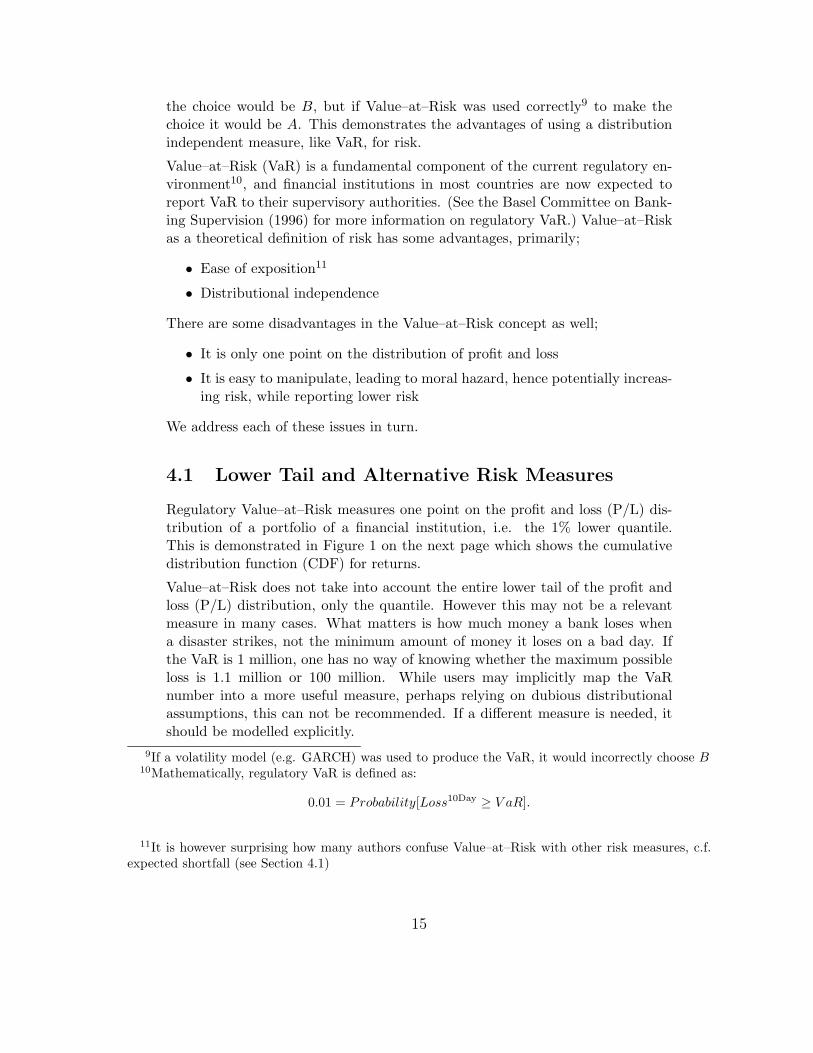
Regulatory Value–at–Risk measures one point on the profit and loss (P/L) dis-tribution of a portfolio of a financial institution, i.e. the 1% lower quantile.This is demonstrated in Figure 1 on the next page which shows the cumulativedistribution function (CDF) for returns.

Value–at–Risk does not take into account the entire lower tail of the profit andloss (P/L) distribution, only the quantile. However this may not be a relevantmeasure in many cases. What matters is how much money a bank loses whena disaster strikes, not the minimum amount of money it loses on a bad day. Ifthe VaR is 1 million, one has no way of knowing whether the maximum possibleloss is 1.1 million or 100 million. While users may implicitly map the VaRnumber into a more useful measure, perhaps relying on dubious distributionalassumptions, this can not be recommended. If a different measure is needed, itshould be modelled explicitly.

9If a volatility model (e.g. GARCH) was used to produce the VaR, it would incorrectly choose B10Mathematically, regulatory VaR is defined as:

0.01 = Probability[Loss10Day ≥ V aR].

11It is however surprising how many authors confuse Value–at–Risk with other risk measures, c.f.expected shortfall (see Section 4.1)

15

Figure 1: Value–at–Risk and the CDF of Profit and Loss

0

1

VaR

1%

In addition, Artzner, Delbaen, Eber, and Heath (1999) note that VaR is nota coherent measure of risk because it fails to be subadditive.12 They proposeto use instead the expected shortfall measure which measures the expected lossconditional on reaching the VaR level. A related measure is the first lower partialmoment which attempts to map the entire lower tail into one number.13

However, this need not to be a serious criticism. As discussed by Cumper-ayot, Danıelsson, Jorgensen, and de Vries (2000) and Danıelsson, Jorgensen, andde Vries (2000), these three risk measures provide the same ranking of riskyprojects under second order stochastic dominance, implying that Value–at–Riskis a sufficient measure of risk. This however only happens sufficiently far the tails.Whether the regulatory 99% is sufficiently far out, remains an open question.14

12A function f is subadditive if f (x1 + ... + xN ) ≤ f (x1) + ... + f (xN ).13The formal definition of expected shortfall is:

∫ t

−∞x

f(x)F (t)

dx.

First lower partial moments:∫ t

−∞(t − x)f(x)dx =

∫ t

−∞F (x)dx.

14Answering this question ought not to be difficult, it only requires a comprehensive empirical study,as the theoretical tools do exist.

16

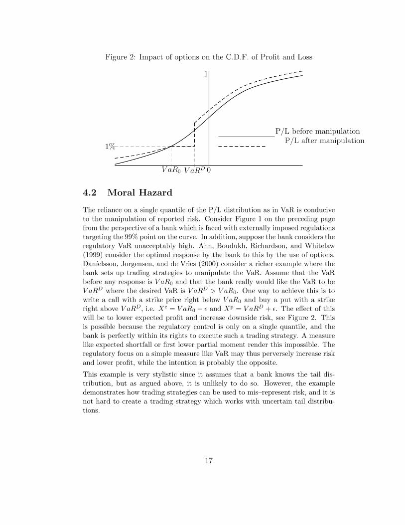
Figure 2: Impact of options on the C.D.F. of Profit and Loss

0

1

V aR0 V aRD

1%P/L after manipulation

P/L before manipulation

4.2 Moral Hazard

The reliance on a single quantile of the P/L distribution as in VaR is conduciveto the manipulation of reported risk. Consider Figure 1 on the preceding pagefrom the perspective of a bank which is faced with externally imposed regulationstargeting the 99% point on the curve. In addition, suppose the bank considers theregulatory VaR unacceptably high. Ahn, Boudukh, Richardson, and Whitelaw(1999) consider the optimal response by the bank to this by the use of options.Danıelsson, Jorgensen, and de Vries (2000) consider a richer example where thebank sets up trading strategies to manipulate the VaR. Assume that the VaRbefore any response is V aR0 and that the bank really would like the VaR to beV aRD where the desired VaR is V aRD > V aR0. One way to achieve this is towrite a call with a strike price right below V aR0 and buy a put with a strikeright above V aRD, i.e. Xc = V aR0 − ε and Xp = V aRD + ε. The effect of thiswill be to lower expected profit and increase downside risk, see Figure 2. Thisis possible because the regulatory control is only on a single quantile, and thebank is perfectly within its rights to execute such a trading strategy. A measurelike expected shortfall or first lower partial moment render this impossible. Theregulatory focus on a simple measure like VaR may thus perversely increase riskand lower profit, while the intention is probably the opposite.

This example is very stylistic since it assumes that a bank knows the tail dis-tribution, but as argued above, it is unlikely to do so. However, the exampledemonstrates how trading strategies can be used to mis–represent risk, and it isnot hard to create a trading strategy which works with uncertain tail distribu-tions.

17

4.3 The Regulatory 99% Risk Level

The regulatory risk level is 99%. In other words, we expect to realize a violationof the Value–at–Risk model once every hundred days, or 2.5 times a year onaverage. Some banks report even lower risk levels, JP Morgan (the creator ofVaR and RiskMetrics) states in its annual report that in 1996, its average daily95% VaR was $36 million. Two questions immediately spring to mind: why wasthe 99% level chosen, and how relevant is it?

The first question may have an easy answer. Most models only have desirableproperties in a certain probability range and the risk level and risk horizon governthe choice of model. For example, at the 95% risk level, conditional normalmodels such as normal GARCH or RiskMetrics are the best choice. However,the accuracy of these models diminishes rapidly with lower risk levels, and at the99% risk level they cannot be recommended, and other, harder to use techniquesmust be employed. In general, the higher the risk level, the harder it is to forecastrisk. So perhaps the 99% level was chosen because it was felt that more extremerisk levels were too difficult to model?

The question of the relevance of a 99% VaR is harder to answer because it dependson the underlying motivations of the regulators. The general perception seemsto be that market risk capital is required in order to prevent systemic failures.However, systemic failures are very rare events, indeed so rare that one has neverbeen observed in modern economies. We have observed near–systemic collapses,e.g. in the Scandinavian banking crisis, but in that case even a meticulouslymeasured VaR would not have been of much help.

The regulatory risk level is clearly mismatched with the event it is supposed tobe relevant for, i.e. systemic collapse. In other words, the fact that a financialinstitution violates its VaR says nothing about the probability of the firms prob-ability of bankruptcy, indeed, one expects the violation to happen 2.5 times ayear. There is no obvious mapping from the regulatory risk level to systemic risk,however defined. Whether there is no link between regulatory risk and systemicrisk is still an open question.

5 Implications for Regulatory Design

The arguments voiced above suggest that modelling as a regulatory tool cannotbe recommended. It does not imply anything about the need to regulate. Bankregulation is a contentious issue which is beyond the scope of this paper. Assum-ing that regulations are here to stay, the important question must be whetherit is possible to create a regulatory mechanism that is successful in reducingsystemic risk, but not too costly.

For most of the 1990s the answer to this question seemed to be risk modelling,

18

and it is only after the Asian and Russian crisis that modelling as a regulatorytool has come under serious criticism. Risk modelling is simply too unreliable,it is too hard to define what constitutes a risk, and the moral hazard issues aretoo complicated for risk modelling to be an integral part of regulatory design,whether for market, credit, or operational risk. This is a reflection of the currentstate of technology.

My analysis focuses on market risk models. Market risk modelling is much easierthan credit risk modelling due to the abundance of accurate market risk dataand more established methodology, compared to the lack of reliable credit riskdata. My criticism applies equally to credit and operational risk models, hencethe case for model based credit and operational regulations is even weaker thanfor market risk.

If the authorities want banks to hold minimum capital, crude capital adequacyratios are the only feasible way. Risk weighing of capital will not work for thesame reason as regulatory risk modelling does not work. However, it is unrealisticto expect banks to meet minimum capital ratios in times of crisis, therefore, suchcapital would have to be state contingent, i.e., a bank would be allowed to runcapital down during crisis. The question what constitutes a crisis, of course stillremains to be answered.

Another possible way is to follow the lead of New Zealand and do away withminimum capital, but require banks instead to purchase insurance, in effectrequire financial institutions to cross insure each other. This market solutionhas the advantage that much more flexibility is built into the system while atthe same time sifting the burden of risk modelling back to the private sector.While such a system may work for small country like New Zealand which caninsure in larger markets, it is still an open question whether this would work forlarger economies.

6 Conclusion

Empirical risk modelling forms the basis of the market risk regulatory environ-ment as well as internal risk control. Market risk regulations are based on usingthe lower 1% quantile of the distribution of profit and loss

(V aR99%

)as the

statistic reported as risk. This paper identifies a number of shortcomings withregulatory Value–at–Risk (VaR), where both theoretic and empirical aspects ofVaR are analyzed.

I argue that most existing risk models break down in times of crisis becausethe stochastic process of market prices is endogenous to the actions of marketparticipants. If the risk process becomes the target of risk control, it changesits dynamics, and hence risk forecasting becomes unreliable. This is especiallyprevalent in times of crisis, such as events surrounding the Russia default of 1998.

19

In practice, Value–at–Risk (VaR) is forecasted using an empirical model in con-junction with historical market data. However, current risk modelling technologystill in the early stages of development, is shown in the paper to be lacking inthe robustness of risk forecasts, and to produce excessively volatile risk forecasts.If risk modelling is not done with great skill and care, the risk forecast will beunreliable to the point of being useless. Or even worse, it may impose significantbut unnecessary costs on the financial institution, due to the misallocation ofcapital and excessive portfolio rebalancing.

This, however, is only a reflection on the current state of technology. A risk modelwhich incorporates insights from economic and financial theory, in conjunctionwith financial data during crisis, has the potential to provide much more accurateanswers by directly addressing issues such as liquidity dynamics. There is a needfor a joint market and liquidity risk model, covering both stable and crisis periods.

The theoretic properties of the VaR measure, conceptually result in VaR pro-viding misleading information about a financial institution’s risk level. The verysimplicity of the VaR measure, so attractive when risk is reported, leaves theVaR measure wide open to manipulation. This in turn implies that foundingmarket risk regulations on VaR, not only can impose considerable costs on thefinancial institution, it may act as a barrier to entry, and perversely increaseboth bank and systemic risk.

The problems with risk modelling have not gone unnoticed. Anecdotal evidenceindicates that many firms employ ad hoc procedures to smooth risk forecasts,and that (some) regulators consider capital as a constant rather than the widelyfluctuating variable suggested by the models. Risk modelling does, however,serve a function when implemented correctly internally within a firm, but itsusefulness for regulatory purposes is very much in doubt.

20

A Empirical Study

The empirical results are a subset of results in Danıelsson (2000). I used there 4common estimation methods

• Normal GARCH

• Student t GARCH

• Historical simulation

• Extreme value theory

as well as representative foreign exchange, commodity, and equity datasets con-taining daily observations obtained from DATASTREAM, from the first recordedobservation until the end of 1999.

• S&P 500 index

• Hang Seng index

• Microsoft stock prices

• Amazon stock prices

• Ringgit pound exchange rates

• Pound dollar exchange rates

• Clean U.S. government bond price index

• Gold prices

• Oil prices

I estimated each model and dataset with a moving 300, 1,000, and 2,000 dayestimation window, and forecast risk one day ahead. Then I record the actualreturn, move the window and reestimate. This is repeated until the end of thesample.

B Scaling Laws

This discussion is partially based on de Vries (1998) and Dacorogna, Muller,Pictet, and de Vries (1999), and it draws on insight from extreme value theory.

The following holds for all iid distributions for which the second moment isdefined.

• The variance of sum is sum of variances V (X + Y ) = 2× V (X) if V (X) =V (Y ) and COV (X, Y ) = 0. This is called self additivity.

If in addition, X is normally distributed, the self additivity property extends tothe tails:

21

• Implication for the quantile: Pr [X ≤ x] = p

– for the sum over two days, the probability of an outcome,

Pr[X1 + X2 ≤ 2

12 x

]= p

– For the sum over T days

Pr[X1 + X2 + ... + XT ≤ T

12 x

]= p

– i.e. V aRT = T12 V aRone day

If however X is iid but not normal, the self additivity property does not applyto the tails, however, even if heavy tailed distributions are typically not selfadditive, the tails are self additive in a special way:

• Consider i.i.d. fat tailed daily returns Xt where Pr [Xt ≤ x] = p

• Then for a sum of the returns

– Pr[X1 + X2 ≤ 2

1α x

]= p

• where α is the tail index

• α is also the number of finite bounded moments

• therefore V aRT = T1α V aRone day

It is known that for financial data α > 2 (if α ≤ 2 the variance is not defined,with serious consequences for much financial analysis). Since we can assume thatthe tail index α > 2, then

T12 > T

1α ,

which has a number of interesting consequences, e.g.

• The use of the square–root–of–time rule to obtain multi–day Value–at–Riskestimates eventually overestimates the risk

• The√

T rule usually used for multi day returns

• For fat tailed data, a T day VaR extrapolated from a one day VaR

V aRT = T1α V aR

Therefore, the√

T rule will eventually lead to an overestimation of the VaRas T increases.

This has implications in other areas besides risk, e.g. in the pricing of pathdependent options, see e.g. Caserta, Danıelsson, and de Vries (1998).

22

C tables

23

Table 1: 99% VaR Violation Ratios 1990–1999

Data Estimation GARCH GARCH Historical Extremehorizon Normal Student-t simulation value theory

S&P–500 300 1.46 1.07 0.79 0.79S&P–500 1, 000 1.27 0.83 0.95 0.99S&P–500 2, 000 0.91 0.67 1.07 1.07

US bond 300 0.94 0.66 0.49 0.49US bond 1, 000 0.53 0.57 0.66 0.41US bond 2, 000 0.37 0.49 0.67 0.37

Oil 300 1.76 1.38 1.17 1.17Oil 1, 000 1.67 1.30 0.92 1.00Oil 2, 000 1.64 1.04 0.35 0.35

Hang Seng 300 2.18 1.41 0.69 0.69Hang Seng 1, 000 1.90 1.29 1.17 1.21Hang Seng 2, 000 2.02 1.21 1.09 1.09

Microsoft 300 2.24 1.78 1.58 1.58Microsoft , 1000 1.98 1.60 1.84 1.74Microsoft 2, 000 2.25 1.69 2.06 1.87

GBP/USD 300 2.13 1.42 0.79 0.79GBP/USD 1, 000 1.85 1.18 0.63 0.63GBP/USD 2, 000 1.62 1.14 0.47 0.47

Notes: Each model was estimated with three different estimation horizons, 300, 1000, and 2000 days.The expected value for the violation ratio is one. A value larger than one indicates underestimationof risk, and a value less than one indicates overestimation. These results are a part of results inDanıelsson (2000)

24

Table 2: S&P–500 Index 1990–1999. VaR Volatility

Risk Statistic Estimation Returns GARCH GARCH Historical ExtremeLevel Horizon Normal Student-t simulation value theory

5% SE 300 0.89 0.47 0.44 0.41 0.415% Min 300 −7.11 −5.32 −4.17 −2.19 −2.195% Max 300 4.99 −0.74 −0.66 −0.73 −0.73

5% SE 2, 000 0.89 0.42 0.41 0.12 0.125% Min 2, 000 −7.11 −3.70 −3.31 −1.55 −1.555% Max 2, 000 4.99 −0.81 −0.74 −1.15 −1.15

1% SE 300 0.89 0.66 0.68 0.71 0.711% Min 300 −7.11 −7.52 −6.68 −3.91 −3.911% Max 300 4.99 −1.05 −1.09 −1.26 −1.26

1% SE 2, 000 0.89 0.60 0.64 0.29 0.331% Min 2, 000 −7.11 −5.23 −5.45 −2.72 −2.841% Max 2, 000 4.99 −1.14 −1.26 −1.90 −1.90

0.4% SE 300 0.89 0.76 0.82 1.94 1.940.4% Min 300 −7.11 −8.58 −8.25 −7.11 −7.110.4% Max 300 4.99 −1.19 −1.36 −1.81 −1.81

0.4% SE 2, 000 0.89 0.68 0.80 0.74 0.630.4% Min 2, 000 −7.11 −5.96 −6.84 −4.27 −4.180.4% Max 2, 000 4.99 −1.30 −1.61 −2.50 −2.49

0.1% SE 300 0.89 0.88 1.06 1.94 1.940.1% Min 300 −7.11 −9.99 −10.92 −7.11 −7.110.1% Max 300 4.99 −1.39 −1.82 −1.81 −1.81

0.1% SE 2, 000 0.89 0.80 1.06 2.10 1.420.1% Min 2, 000 −7.11 −6.94 −9.31 −8.64 −7.490.1% Max 2, 000 4.99 −1.52 −2.26 −3.13 −3.15

Notes: For each model and the risk level, the table presents the standard error (SE) of the VaRforecasts, and the maximum and minimum forecast throughout the sample period. These results area part of results in Danıelsson (2000)

25

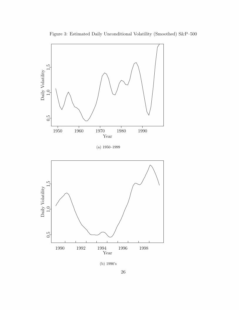
Figure 3: Estimated Daily Unconditional Volatility (Smoothed) S&P–500

Daily

Volatility

Year1950 1960 1970 1980 1990

0.5

1.0

1.5

(a) 1950–1999

Daily

Volatility

Year1990 1992 1994 1996 1998

0.5

1.0

1.5

(b) 1990’s

26

Figure 4: Daily Hang Seng Index 1997 and 99% VaR

-20

-15

-10

-5

0

5

10

15

20

09/13 09/27 10/11 10/25 11/08 11/22 12/06 12/20

ReturnsGARCH

EVT

Figure 5: Which is More Volatile and which is more Risky?

Returns

−6%

−4%

−2%

0%

2%

(a) Returns A

Returns

−6%

−4%

−2%

0%

2%

(b) Returns B

27

References

Ahn, D. H., J. Boudukh, M. Richardson, and R. F. Whitelaw (1999):“Optimal Risk Management Using Options,” J. Finance, 54 (1), 359–375).

Andersen, T., and T. Bollerslev (1998): “Answering the Skeptics: Yes,Standard Volatility Models Do Provide Accurate Forecasts,” InternationalEconomic Review, 38, 885–905.

Artzner, P., F. Delbaen, J. Eber, and D. Heath (1999): “Coherent Mea-sure of Risk,” Mathematical Finance.

Basel Committee on Banking Supervision (1996): Overview of the amand-ment to the capital accord to incorporate market risk.

Caserta, S., J. Danıelsson, and C. G. de Vries (1998): “Abnormal Return,Risk, and Options in Large Data Sets,” Statistica Neerlandica, November.

Christoffersen, P. F., and F. X. Diebold (2000): “How Relevant is Volatil-ity Forecasting for Financial Risk Management?,” Review of Economics andStatistics, 82, 1–11.

Cumperayot, P. J., J. Danıelsson, B. N. Jorgensen, and C. G. de Vries

(2000): “On the (Ir)Relevancy of Value–at–Risk Regulation,” Forthcommingbook chapter: Springer Verlag.

Dacorogna, M. M., U. A. Muller, O. V. Pictet, and C. G. de Vries

(1999): “Extremal foreign exchange rate returns in extremely large data sets,”www.few.eur.nl/few/people/cdevries/workingpapers/workingpapers.htm.

Danıelsson, J. (2000): “(Un)Conditionality and Risk Forecasting,” Unfinishedworking paper, London School of Economics www.RiskResearch.org.

Danıelsson, J., P. Hartmann, and C. G. de Vries (1998): “The cost ofconservatism: Extreme returns, Value-at-Risk, and the Basle ’MultiplicationFactor’,” Risk, January 1998, www.RiskResearch.org.

Danıelsson, J., B. N. Jorgensen, and C. G. de Vries (2000):“Risk Managements and Complete Markets,” Unfinished working paper,www.RiskResearch.org.

Danıelsson, J., and R. Payne (2000): “Real Trading Patterns and Prices inSpot Foreign Exchange Markets,” working paper www.RiskResearch.org.

de Vries, C. G. (1998): “Second Order Diversification Effects,”www.few.eur.nl/few/people/cdevries/workingpapers/workingpapers.htm.

Drost, F. C., and T. E. Nijman (1993): “Temporal Aggregation of GARCHProcesses,” Econometrica, 61, 909–927.

Dunbar, N. (1999): Inventing Money: The Story of Long–Term Capital Man-agement and the Legends Behind It. John Wiley.

28

Economist (1998): “Risk management. Too clever by half,” The Economist,pp. 140–145.

Erb, Harvey, and Viskanta (1994): “Forecasting International Correla-tions,” Financial Analysts Journal.

Froot, K. A., D. S. Scharfstein, and J. C. Stein (1993): “Risk Man-agemnt: Coordinating Corporate Investments and Financing Policies,” J. Fi-nance, XLVIII, no 4, 1629–1658.

Goodhart, C. A. E. (1974): “Public lecture at the Reserve bank of Australia,”reprinted.

Hartmann, P., S. Straetmans, and C. G. de Vries (2000): “Asset MarketLinkages in Crisis Periods,” working paper.

Jacobs, B. (1999): Capital Ideas and Market Realities. Blackwell.

Longin, F. (1998): “Correlation structure of international equity markets dur-ing extremely volatile periods,”babel.essec.fr:8008/domsite/cv.nsf/WebCv/Francois+Longin.

McNeil, A. J., and R. Frey (1999): “Estimation of Tail–Related RiskMeasures for Heteroskedastic Financial Time Series: An Extreme Value Ap-proach,” Journal of Emprical Finance, forthcoming.

Morris, S., and H. S. Shin (1999): “Risk Managementwith Interdependent Choice,” Mimeo Nuffield College, Oxfordhttp://www.nuff.ox.ac.uk/users/Shin.

Stahl, G. (1997): “Three cheers,” Risk, 10, 67–69.

29