1

The Emergence of Financial

Cryptography.

An analysis of Bitcoin and its viability as a currency using a

GARCH model of volatility.

University of Surrey

Kern Robinson

Ralph Clayton

Robert Muddle

Roman Gregory

Thomas Leach

Vincent Yau

Vladimir Emelianov

13th May 2014

2

Abstract

With all of the recent hysteria surrounding the emergence of crypto-currencies, this

paper assesses the viability of Bitcoin through estimating its volatility whilst

hypothesizing its place in society as a viable currency. We have used an econometric

estimation method known as ARCH/GARCH in order to assess the volatility of the

currency in order to analyse it’s viability against the six characteristics of a currency.

This paper concludes that Bitcoin is in fact a viable currency, however it is still in the

early stages of development and to succeed long term will have to address its high

volatility.

3

Contents

1. Introduction 4

2. Money; a brief background. 6

3. Literature Review 8

4. Methodology

4.0 The ARCH/GARCH Model. 12

4.1 Conditions for ARCH/GARCH Model 13

4.2 Variable & Distribution Selection. 14

4.3 Interpreting the Coefficients. 17

5. Findings 17

6. Conclusion 19

7. Appendix 21

8. Reference list 26

4

1. Introduction.

Currency is a term to describe a medium of exchange between parties in return for

goods or services. Many different types of currency have been used throughout

history; these include commodities, hard money, and fiat money. Recently, crypto-

currencies have become a widely debated topic regarding their place in today’s

society1. The most well-known and successful crypto-currency is Bitcoin, which will

be the topic of this paper

What is Bitcoin?

Bitcoin is a peer-to-peer digital currency, introduced in 2009 by a developer

supposedly known as Satoshi Nakamoto. It is decentralised meaning there is no-one

who owns or regulates it; instead details of all transactions are recorded in a shared

public ledger known as the block chain.

It works through each user owning a digital wallet on their computer, which stores the

addresses of each Bitcoin contained in that wallet. To send a Bitcoin to another

wallet, the platform takes the previous owner’s address, as well as that of the wallet

the Bitcoin is being sent to, these details will be submitted to the block chain and

confirmed by the network within 10 minutes through the process of mining. Mining is

the process of compiling all the recent transactions into a block and added to the block

chain. The quickest miner to do this is rewarded with 25 newly created Bitcoins. This

serves as the only way Bitcoins are created, which means the issue of Bitcoins is

controlled by an algorithm as opposed to a central bank. The algorithm is designed to

mimic the rate in which commodities such as gold are mined. The amount of Bitcoins

awarded halves every 210,000 blocks, and is capped at a total of 21million Bitcoins. 2

1 The Economist, (2011). Bits and bob. [online] Available at:

http://www.economist.com/node/18836780 [Accessed 8 May. 2014]. 2 Bitcoin.org, (2014). How does Bitcoin work? - Bitcoin. [online] Available at:

https://bitcoin.org/en/how-it-works

5

The demand for Bitcoin

One of Bitcoin’s main attractions is its decentralised system; this allows users to

freely make transactions without charges being made to a middleman. Another benefit

of this is that it means the user owns their Bitcoins, with no central authority being

able to take ownership. Bitcoin is also used because it’s fast; transactions are

confirmed within 10 minutes, allowing users to transfer large sums without having to

wait a few days; which is typical with most bank transfers. There are many other

advantages such as no chargebacks, which is a common case for credit card fraud and

the personal information of users is safe; most other forms of online payments require

large amounts of personal information which could potentially be stolen.3

Why is Bitcoin being so heavily debated?

The underlying issue with many users, both current and future, is the uncertainty of

what is to become of Bitcoin. A Bitcoin is just a string of digital code, with the value

depending on what other users are willing to pay for it, which in turn is reliant on the

belief Bitcoin will still be used as a currency in the future. This is true with most fiat

currencies being used today, but there is one main difference with Bitcoin: the fact it

has not been made legal tender by a Government.4

The focus of this paper surrounds the likely future of Bitcoin. We aim to predict this

through identifying, evaluation and comparing key characteristics of Bitcoin

compared with currently used fiat currencies.

The context in which ‘viable’ is used in this paper will refer to the prospect of Bitcoin

being used in the long run whilst satisfying the demand for digital currency.

3 The Economist (2011), Bits and bob [online] Available at:

http://www.economist.com/blogs/babbage/2011/06/virtual-currency [Accessed 1st May 2014]

4 Hoppe (1994),The Review of Austrian Economics, Volume 7, Issue 2, pp 49-74

6

2. Money; a brief background.

It is hypothesised across several academic papers that there are six characteristics a

currency should possess if it is going to be viable, these are: durability, portability,

divisibility, uniformed, limited supply, and acceptability. 56

Originally, currencies were backed by commodities, such as gold standard.

Today, currencies are fiat money; non-redeemable paper money that is made legal

tender by the government of a specific country. The portability and durability of fiat

money made it more convenient thus fiat money became widely used.

These characteristics serve as a good base for evaluating the future of Bitcoin.

Durability: with Bitcoins being made up of a string of code, they could be traded an

infinite amount of times without losing integrity. However, through human error,

Bitcoins could be lost, as they are stored on individual computers, if that computer

was to crash or the data erased, the Bitcoins would be lost forever.

Portability: Wallets can be setup in minutes and transactions are made quickly, with

the log formed into the blockchain within 10 minutes, with no third-parties needed for

authorisation.

Divisibility: Bitcoins can be divided into units of 8 decimal places (Satoshis). If

necessary, the code could be updated to allow further division, making Bitcoin

infinitely divisible

Uniformed: Bitcoins are identical, with each Bitcoin being an exact replica of all

others.

5 Rothbard, M. (1983). The mystery of banking. 1st ed. New York, N.Y.: Richardson & Snyder. 6 Bagus, P. (2009). THE QUALITY OF MONEY. Quarterly Journal of Austrian

Economics, 12(4).

7

Limited supply: a fixed amount brought into supply every 10minutes up until the limit

is reached.

Acceptability: Fiat currencies have the benefit that once they have been made legal

tender, they instantly become accepted. Bitcoin acceptance is slowly increasing;

whether it will become widely accepted depends on many factors.

As shown, Bitcoin fits five of the six characteristics extremely well, however falls

behind significantly on the acceptability aspect. For Bitcoin to become viable it needs

to develop a larger user base consisting of both businesses and individuals. For the

larger part of the paper, we will evaluate academic papers to assess the key factors

that will affect the acceptability and therefore viability.

A key aspect affecting the acceptability of Bitcoin is the volatility of the currency;

High volatility is an issue as users won’t want to be exposed to the resulting risks.

Any user relying on Bitcoin as an income would prefer a stable, predictable income.

Our research has led us to estimating the volatility using an econometric estimation

method known as ARCH/GARCH regression, the details of which are specified later

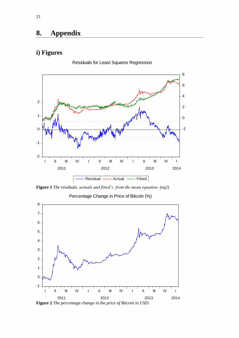
on. It is possible to see Bitcoin is highly volatile just by looking at the percentage

price change (See figure 2), however we decided to derive a more explicit explanation

of volatility.

8

3. Literature Review.

This review discusses published evidence debating both the significant factors related

to the characteristics of viable currency and factors likely to affect the acceptability of

Bitcoin. We will be specifically looking at the confidence, volatility and legalities of

Bitcoin to assess the acceptability, reviewing literature on the ARCH/GARCH model

and the continuing debate with regard to Bitcoin viability.

Given Bitcoin’s relatively youthful existence, first published in 2009, there is a

limited spectrum of literature on it; more specifically, it’s viability. Therefore, we

begin by looking at publications that identify key characteristics of money.

3.1 Confidence

For many, confidence and expectations are pivotal in assuring a currencies’ longevity.

Simmel, in regards to new money, claims “the acceptance of money cannot develop

without public confidence.” (Selgin, 1994)7 this relates to Bitcoin in that without

confidence, it will surely fail as a currency. Although an opinion, Simmel’s attitude

towards confidence is a widely supported school of thought in economics.

In addition, “Simmel feared that abuse of monetary systems by governments would

lead to the breakdown of trust, which depends among other things on confidence in

the future stability of money’s purchasing power.” (Selgin, 1994) Selgin explains how

confidence in a currency, and its’ purchasing power, is crucial to prevent a currency

from crashing. What differs in Bitcoin is that it is non–centralised. Thus, the stability

of a government or the “trust” in the government should not affect the stability of

purchasing power in the same way. Bitcoin’s code is open source and anyone can

verify how Bitcoin works, thus users of Bitcoin need not trust a central body, but will

still need to have confidence in the future purchasing power of Bitcoin.

7 Selgin.G (1994), On Ensuring the Acceptability of a New Fiat Money, Journal of Money, Credit and

Banking, Vol. 26, No. 4, Pg 808 - 826

9

One could suggest however, that without the backing of a government there will be

less initial support and trust in a non-centralised currency. Later we will see, in

relation to centralised currencies, how volatile Bitcoin appears to be and how this

affects confidence of future purchasing power.8

3.2 Volatility

In order to begin estimating how volatile Bitcoin is, we decided to use an estimation

method known as ARCH/GARCH.

The ARCH model was derived and published in 1982 by Economist Robert Engle as

a method of analysing economic time series with time-varying volatility9. His work

on the ARCH model, for which he won a Nobel Prize in 2003, and other statistical

models have become essential tools in economics ever since.

Following on from the ARCH process introduced in Engle (1982), economist

Bollerslev developed the model and introduced the GARCH model, Bollerslev

(1986) 10 . The GARCH model, explained later, has become fundamental when

modelling time dependent volatility. So much so, that it has been referred to as “the

workhorse of the industry” (Lee & Hansen 1994)11.

Given the pivotal nature of these processes in Economics and that they have been

accepted and widely utilized for many years, we are confident it is the appropriate

technique for our model on volatility.

8 Bitcoin.org, (n.d.). FAQ - Bitcoin. [online] Available at: https://bitcoin.org/en/faq#why-do-people-trust-bitcoin. 9 Engle R (1982), Autoregressive Conditional Heteroskedasticity, Econimetrica, Vol. 50, No.4 10 Bollerlslev T (1986), Generalized Autoregressive Conditional Heteroskedasticity, Journal of Econometrics 31 11 Lee S & Hansen B (1994) , Asymptotic Theory for the GARCH (1,1) Quasi-maximum Likelihood

Estimator

10

3.3 Bitcoin Debate

A recent paper on Bitcoin and its future (Bollen, 2013)12, focusing on the legality of

digital currencies, suggests that in the long run Bitcoin can and probably will succeed

in becoming a viable currency. This attitude was not shared by Krugen who argued

crypto-currencies were so “vulnerable to economic factors such as money hoarding,

deflation and depression” that they would not succeed in the long run. (Krugen,

2011)13 Given Krugen wrote this in 2011, when Bitcoin was still young and relatively

unproven, one can understand his dismissal of Bitcoin long term viability. The

multiple thefts and crashes that have occurred are evidence of the vulnerability that

Krugen spoke of and to an extent foresaw. However, with the benefit of hindsight one

can argue that Bitcoin has developed many fail safes to supersede its failures.

Multiple times Bitcoin has fallen foul to one of its weaknesses and yet has bounced

back and survives to this day.

Bollen’s paper, although useful in aiding our research on Bitcoin viability, mainly

focuses on the legal and regulatory side of Bitcoin and its uses. We cannot therefore

fully rely on this analysis as supporting the economic viability; these aspects will

however affect acceptability.

According to Patterson (2013), in an article on the Foundation for Economic

Education website, Bitcoin is a currency that possesses the necessary attributes to be

viable. Patterson argues that Bitcoin shares many fundamental properties with both

gold and silver.14 Given the success of gold and silver, the similarities, in Patterson’s

opinion, give Bitcoin good foundations for success. Furthermore, Patterson agrees

Bitcoin outperforms gold and silver in some aspects; both its portability and

divisibility as previously mentioned.

While the article by Patterson is relevant to our research, he does not go into much

depth in terms of economic theory, nor does he analyse any data to support his

12 Bollen.R (2013), Conclusions and Recommendations, The legal status of online currencies; are

Bitcoins the future? 13 KrugenP (2011), “Golden Cyberfetters”, New York Times, “ 7 September 2011 (krugman.blogs.ny

times.com/2011/09/07/golden-cyberfetters, accessed 30 April 2014) 14 Patterson.S (2013), “Is bitcoin a viable currency?”, Foundation for Economic Education, 11

December 2013 (www.fee.org/the_freeman/detail/is-Bitcoin-a-viable-currency, assessed 30 April

2014)

11

opinion. The article is mainly speculation and would require further analysis in order

to draw sound conclusions. Despite these drawbacks, we believe Patterson is helpful

as he points us in a positive direction.

Economist Gary North, in 2013 claimed that Bitcoin was a Ponzi scheme, a fraudulent

investment scheme in which the creators benefit from individuals who believe the

system to be an arbitrage opportunity to make money. Perhaps one of the most well

regarded economists to have commented on Bitcoin as a currency, North clearly

disagrees with the notion that it can be viable in the long term (North, 2013)15. North

analyses what is meant by money through looking at Menger’s On the Origin of

Money, 1892. In contrast to the aforementioned, Bollen and Patterson, North strictly

disagrees that Bitcoin satisfies the characteristics that define money therefore

eliminating its viability as a currency.

North argues that due to its volatility, people will hang on to Bitcoin rather than

exchanging them for goods. This does seem to be a feasible idea; many people have

made significant gains through buying and selling their Bitcoin, rather than

exchanging them. Individuals and firms, as North suggests, might believe there to be

more value in holding on to Bitcoin as a commodity rather than using them as

currency. From this he draws the overwhelming conclusion that Bitcoin is not money,

and will never succeed as a currency.

Although there has been criticism of North’s radical view that Bitcoin is a Ponzi

scheme, as an established and well supported economist, he has received some

support from the wider community. North’s opinion completely opposes the notion

that Bitcoin can be a viable currency. In this paper we aim to formulate our own

opinion on a more analytical level.

15 North.G (2013), “Bitcoins: The Second Biggest Ponzi Scheme in History”, 29 November

2013(http://www.garynorth.com/public/11828.cfm, assessed 30 April 2014)

12

4. Methodology

4.0 The ARCH/GARCH Model.

Autoregressive Conditional Heteroskedasticity (ARCH) models are used to

characterize and model observed time series. The concept introduced by Engle

(1982) 16 , could be effectively applied to time series models with conditional

heteroskedasticity. Engle put forward the idea that information from a previous period

(t-1) could impact the conditional disturbance variance (volatility). He concluded the

following:

𝜎𝑢𝑡2 = 𝛼0 + 𝛼1𝑢𝑡−1

2 + ⋯ + 𝛼𝑝𝑢𝑡−𝑝2 (eq. 1)

The variance equation (eq.1) portrays the volatility from the previous period

measured in the lags of the squared residuals, derived from a mean equation. The

conditional disturbance variance is the variance of 𝑢𝑡 ; it is conditional upon

information available up to time t-1, determined below.

𝜎𝑢𝑡2 = 𝑉𝑎𝑟(𝑢𝑡 | 𝑢𝑡−1, … , 𝑢𝑡−𝑝)

= 𝐸(𝑢𝑡2 | 𝑢𝑡−1, … , 𝑢𝑡−𝑝)

The mean equation is the equivalence of the desired dependent variable as a function

of its regressors. In the model we propose, the mean equation will be expressed as;

𝑙𝑛𝑏𝑡𝑐 = 𝛽0 + 𝛽1𝑙𝑛𝑏𝑡𝑐𝑣𝑜𝑙 + 𝛽2𝑙𝑛𝑐𝑝𝑡 + 𝛽3𝑙𝑛𝑑𝑖𝑓𝑓 + 𝑢 (eq.2)

The GARCH model (Generalised Autoregressive Conditional Heteroskedasticity) was

proposed by Bollerslev (1986)17. Bollerslev’s publication exposed that the GARCH

with a lesser number of terms can perform as well as or better than an ARCH model

with several parameters. The GARCH model inherits an additional component to the

16 Engle, R. (1982). Autoregressive conditional heteroscedasticity with estimates of the variance of United Kingdom inflation. Econometrica: Journal of the Econometric Society, pp.987--1007. 17 Bollerslev, T. (1986). Generalized autoregressive conditional heteroskedasticity. Journal of econometrics, 31(3), pp.307--327.

13

variance equation, the variance of the lagged residuals (𝛾𝑡𝜎𝑢𝑡−12 ). An equation in the

form GARCH (p,q), shown below.

𝜎𝑢𝑡2 = 𝛼0 + 𝛼1𝑢𝑡−1

2 + 𝛾𝑡𝜎𝑢𝑡−12 + ⋯ + 𝛼1𝑢𝑡−𝑝

2 + 𝛾𝑡𝜎𝑢𝑡−𝑞2 (eq.3)

4.1 Conditions for ARCH/GARCH Model

We will focus on two conditions that sustain that the ARCH/GARCH model can be

applied to our data.

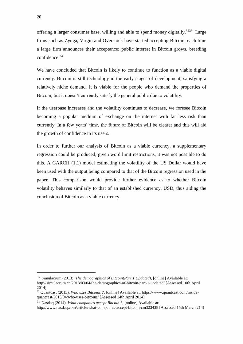
4.1.1 Volatility Clustering

Volatility clustering states that period of high variance are often followed by further

periods of high variance and vice versa for ambient periods of low volatility

Mandelbrot (1963) 18 and Fama (1965) 19 . Empirical evidence suggests that an

ARCH/GARCH model can be applied to data that exhibits this characteristic. Figures

1 and 2 both show that the residuals of mean equation (1) display this autocorrelation

between periods. We may therefore verify that the ARCH/GARCH model can be

applied to our model.

4.1.2 ARCH Test Hypothesis

The second of the conditions to be met is an ARCH test which can be executed on

eviews. Fundamentally the ARCH test hypothesis states the following:

H0: There is no ARCH effect.

H1: There is an ARCH effect.

The test is implemented in the following way; regress the desired dependent variable

on its regressors to obtain the mean equation (eq. 2). Save the residuals and perform a

regression of the residual squared on its lagged counterparts. For the following

equation:

18 Mandelbrot, B. (1963). The Variation of Certain Speculative Prices. The Journal of Business, 36(4), pp.394-419 19 Fama, E. F. (1965). The behavior of stock-market prices. Journal of business, 34-105.

14

�̂�𝑡2 = �̂�0 + �̂�1𝑢𝑡−1

2 + ⋯ + �̂�𝑝𝑢𝑡−𝑝2 (eq.4)

𝑝 determining the chosen number of lags.

We test for heteroskedasticity, the null hypothesis states that over time the conditional

disturbance variance is constant, the alternative hypothesis states that at time 𝑡 the

variance is partial to the conditional disturbance variance of the previous 𝑝 periods.

𝐻0: �̂�1 = �̂�2 = ⋯ = �̂�𝑝

𝐻1: �̂�1 ≠ �̂�2 ≠ ⋯ ≠ �̂�𝑝

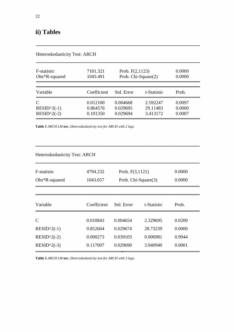
We selected to test at 1, 2, 3 & 4 lags. When tested at 1 and 2 lags the chi-squared

statistic was significant, likewise were the two ARCH coefficients. At 3 and 4 lags the

chi-squared statistic was significant. However, at 3 lags the 2nd lag residual coefficient

becomes insignificant; similarly at 4 lags the 2nd and 3rd residual coefficients are

insignificant. Thus, we chose to select to use ARCH order 2.

Testing for a GARCH (1,1) is locally equivalent to performing a test for ARCH(1)

(for proof see, Jondeau et al, p.92, 2007)20. Therefore we elect to use a GARCH (2,2).

4.2 Variable & Distribution Selection.

To model the volatility we have decided it is best to go forth with the ARCH/GARCH

model as discussed above. To construct the GARCH model we must first look at the

initial mean equation (eq.2) to identify explanatory variables we would like to include

in our primary regression. To find the most appropriate variables, using available

data, we intuitively identified what factors can explain the price of Bitcoin itself. The

explanation behind using these regressors follows.

20 Jondeau, E., Poon, S. and Rockinger, M. (2007). Financial modeling under non-gaussian distributions. 1st ed. London: Springer, p.92.

15

Cost Per Transaction, we hypothesized that an increase in the cost of transacting

Bitcoins would have a negative impact on price as users decide to restrict their use of

the currency as the cost of transacting increases, this would therefore result in a

decrease in the price of Bitcoins

The difficulty variable describes the difficulty of mining Bitcoins i.e. how long it

would take to complete a block. The difficulty level would have a positive impact on

the price as an increase in the level of difficulty can be seen as a narrowing of the

supply of currency, under regular economic theory narrowing of supply would result

in a stronger or more valued currency.

Volume describes how many Bitcoins were transacted throughout the day. The output

volume would have a positive relationship with the price level; with higher

transaction volumes, the price would also see higher levels.

The second component of the equation is the variance equation (eq.3). The variance

equation comprises of the ARCH/GARCH terms plus the rate of return for the

EURUSD rate and the rate of return for the GBPUSD exchange rate. This was

achieved by taking the log of the linear exchange rates. Concluding that the ideal

model was GARCH(2,1) the variance equation is illustrated below.

𝜎𝑏𝑡

2 = 𝛼0 + 𝛼1𝑏𝑡−12 + 𝛼2𝑏𝑡−2

2 + 𝛾1𝜎𝑏𝑡−1

2 + 𝛾2𝜎𝑏𝑡−2

2 + 𝛽1𝑙𝑛𝑒𝑢𝑟𝑡 + 𝛽2𝑙𝑛𝑔𝑏𝑝𝑡 (eq.5)

We decided to use some of the world’s largest and widely used currencies, the USD,

GBP and the EUR. Accumulatively, these currencies make up almost 90% of the

world’s reserve currency, with GBP being central to financial markets21, while the

EUR and US are some of the world’s largest economies and make up more than 80%

of the world’s reserve currencies22. The reasoning behind using these currencies in the

variance equation is as follows: An increased period of volatility in the value of a

21 Archive.today, (2006). Xak.com: Currency Strategists: Morgan Says Pound Is Euro Proxy. [online] Available at: http://archive.today/Hkb6X#selection-852.35-852.38 [Accessed 6 May. 2014]. 22 IMF, (n.d.). Currency Composition of Official Foreign Exchange Reserves (COFER). [online] Available at: http://www.imf.org/external/np/sta/cofer/eng/cofer.pdf.

16

currency can be linked to macroeconomic instability.23(i.e. inflation, volatile growth,

etc), as a result of this instability and volatility speculators may begin to panic, with

Bitcoin’s role as a speculative vehicle, this may result in increased instability and

volatility in the price of Bitcoin.

4.2.1 Error Distribution

When constructing a GARCH model on eviews, there are three approaches in which

the errors can be distributed, Gaussian (Normal), Student’s t or Generalised Error

(GED). Due to the stigma of volatility that Bitcoin infamously inherits, a

characteristic which is palpable in the raw data gathered in Figures 1 & 2 (see

Appendix, i), we can assume the data is non-normal and not i.i.d (independent and

identically distributed). Therefore normality can be rejected, this can be explained

financially, by the assumption that the factors affecting the value of an asset or price

are ‘well-behaved’ (Mandelbrot 1963)24. It is known the factors affecting Bitcoin do

not possess this quality. Assuming that our data most probably has a leptokurtic

distribution (‘fat-tailed’), the student’s t or GED could be suitable25. For simplicity,

we choose to continue with the student’s t distribution as this is perfectly capable of

satisfying the requirements for the distribution of our error.

4.2.2 Adjustments

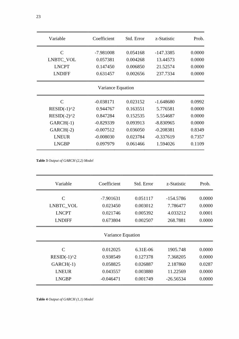
After computing our output using the GARCH (2,2) model, we found some of the

coefficients produced were insignificant, namely the 𝛾2𝜎𝑢𝑡−22 , the second lag of the

GARCH term, shown in Table 3 (see Appendix, ii). The implication being that the

conditional disturbance variance of 2 previous periods could not have an effect on

current period volatility. To rectify this error in our model we decided to take the

model back to a GARCH (1,1) model, in this case all of our predicted coefficients are

significant, shown in Table 4 (see Appendix, ii).

23 Sciencedirect.com, (2009). On the macroeconomic causes of exchange rate volatility. [online] Available at: http://www.sciencedirect.com/science/article/pii/S0169207009000375 [Accessed 6 May. 2014]. 24 Mandelbrot, B. (1963). The Variation of Certain Speculative Prices. The Journal of Business, 36(4), pp.394-419. 25 Giller, D. (2009). Why Use the Generalized Error Distribution?. [online] Blog.gillerinvestments.com. Available at: http://blog.gillerinvestments.com/post/2009/3/19/Why-Use-the-Generalized-Error-Distribution.aspx [Accessed 7 May. 2014].

17

4.3 Interpreting the Coefficients.

With reference to Table 4 (see Appendix, ii), our final regression analysis, we can

infer from the output the following:

The ARCH term (RESID(-1)^2 in Table) shows a trait of an asset which can be

extremely erratic. A stable asset would tend to exhibit a value between 0.05 and 0.1,

as we can see in our output this is at 0.94 (2.s.f). This is considerably larger than a

stable asset exposing the excessive amount of volatility in Bitcoin. The GARCH term

(GARCH(-1) in Table) gives an indication of the persistence of a volatility shock,

stable assets would tend to produce a value around 0.85 and 0.98 26. Naturally, as we

have a high ARCH term our GARCH term will lower, due to 𝛼1 + 𝛾1 ≤ 1.27 As the

table denotes we have a GARCH coefficient of 0.059 (2.s.f) this shows that

persistence in the shocks is minimal and tend not to last longer than one period.

The currency pair (LNEUR and LNGBP in Table) coefficients show how a

percentage point change in the EURUSD and GBPUSD affect the volatility of

Bitcoin. A percentage point change in the Euro accounts for a 0.044 (2.s.f) change in

the conditional disturbance variance (volatility) of Bitcoin, whereas the GBP accounts

for a -0.046 (2.s.f) change in Bitcoin’s volatility.

5. Findings

In this section we will make a reference to the works of Engle and Patton

(2001)28 and Carroll (2011)29. This will give us the benefit of comparing the

magnitude in the scale of volatility between Bitcoin, Dow Jones and ISEQ. The

26 Alexander, C. (2008). Market risk analysis. 1st ed. Chichester, England: Wiley, p.283. 27 Engle, R. (2001). GARCH 101: The use of ARCH/GARCH models in applied econometrics. Journal of economic perspectives, pp.157--168. 28 Engle, R. and Patton, A. (2001). What good is a volatility model. Quantitative finance, 1(2), pp.237--245. 29 Carroll, T. and Collins, J. (2012). Volatility models and the ISEQ index

18

two pieces of work adopt a similar empirical approach to our work, which we

can use to make inference upon our own output.

The 𝛼1 + 𝛾1 values for the GARCH models in the 3 studies represent the

equations mean reversion to its long run variance as this figure approaches 1 the

longer the volatility will take to converge back to its mean. In Engle and Patton’s

study this value is 0.9904 for the Dow Jones and in Carrol’s study 0.974. Carrols

study made inference to the fact that the Dow Jones would take longer to

approach it’s long run variance. Our study returned a figure of 0.997, which gives

evidence of an even more gradual mean reverting process.

Another measure to compare the mean reverting process is the half-life

prediction (for calculation, see appendix, iii, EQ6). The half-life is the time it

takes for the volatility of Bitcoin to decrease by half towards it’s mean value.

Comparing Bitcoin’s half-life to that of the Dow Jones’ half-life we find that

Bitcoins have a considerably higher half-life of 265 days in contrast to the Dow’s

half-life is estimated to be 73 days by Engle and Patton and 28 days by Carroll for

the ISEQ. The extortionately larger half-life of Bitcoins, shows that an isolated

shock, following no further shocks (which is quite a strong assumption) the

isolated shock will take a longer period of time to dissipate. In this case the it

would take more than 3 times as many days for the effect of a shock Bitcoin to

feed through in comparison to the Dow Jones. 265 days is an considerably long

time for an effect of a shock to feed through and could be interpreted as

insignificant as this result may be skewed by the fact we know our 𝛼1 value is

around 18 times larger than Carrols values gathered for the ISEQ, displaying a

greater frequency of shocks.

This high 𝛼1 value, in table 4 (see appendix, ii), displays that even for the more

informed users of Bitcoin the price can be difficult to predict for the next period.

Unpredictable volatility similar to this has been seen in historical periods such as

the hyperinflation in the Weimar Republic after the First World War, where the

19

currency was abandoned as normal economic transactions became difficult to

facilitate under the Mark’s tenure.30

6. Conclusion

There has been much excitement and controversy surrounding the emergence of

Bitcoin, with policy makers viewing Bitcoin as a useful financial product and

speculators enjoying large returns. Crypto-currencies are a relatively new product in

the marketplace; consequently there has been little research in this area. This paper

assesses the viability of Bitcoin through estimating its volatility whilst hypothesizing

its place in society as a viable currency.

Our model of volatility estimation concluded that Bitcoin is a highly volatile currency.

Based on the ARCH/GARCH regression we conducted; our results stated that the

volatility of the price of Bitcoin is highly sensitive to any exogenous shock that may

occur to the price. We were also able to conclude that the crypto-currency exhibited

large amounts of volatility clustering and price fluctuations.

Furthermore, looking at calculations already carried out in other papers, it is possible

to see that the volatility is steadily decreasing at a rate of “.00008 a day, or about 3

percentage points annually.31

To work effectively as a medium of exchange and be widely accepted in the long run

the volatility will need to continue decreasing, otherwise the user base will be limited

to few firms who are willing to accept Bitcoin.

With larger transaction volume and more firms adopting Bitcoin, it is likely the

volatility will continue to drop. Many firms have caught on as the demographics of

Bitcoin users are young, digitally affluent users with higher-than-average incomes,

30 Fergusson A (1975). When money dies. 1st ed. London: Kimber. 31 Cryptonomics (2014). Is Bitcoin volatility really in decline? [online] Available at: http://cryptonomics.org/2014/01/22/is-bitcoin-volatility-really-in-decline/ [Assessed 9th May 2014]

20

offering a larger consumer base, willing and able to spend money digitally.3233 Large

firms such as Zynga, Virgin and Overstock have started accepting Bitcoin, each time

a large firm announces their acceptance; public interest in Bitcoin grows, breeding

confidence.34

We have concluded that Bitcoin is likely to continue to function as a viable digital

currency. Bitcoin is still technology in the early stages of development, satisfying a

relatively niche demand. It is viable for the people who demand the properties of

Bitcoin, but it doesn’t currently satisfy the general public due to volatility.

If the userbase increases and the volatility continues to decrease, we foresee Bitcoin

becoming a popular medium of exchange on the internet with far less risk than

currently. In a few years’ time, the future of Bitcoin will be clearer and this will aid

the growth of confidence in its users.

In order to further our analysis of Bitcoin as a viable currency, a supplementary

regression could be produced; given word limit restrictions, it was not possible to do

this. A GARCH (1,1) model estimating the volatility of the US Dollar would have

been used with the output being compared to that of the Bitcoin regression used in the

paper. This comparison would provide further evidence as to whether Bitcoin

volatility behaves similarly to that of an established currency, USD, thus aiding the

conclusion of Bitcoin as a viable currency.

32 Simulacrum (2013), The demographics of Bitcoin(Part 1 Updated), [online] Available at:

http://simulacrum.cc/2013/03/04/the-demographics-of-bitcoin-part-1-updated/ [Assessed 10th April

2014] 33 Quantcast (2013), Who uses Bitcoins ?, [online] Available at: https://www.quantcast.com/inside-

quantcast/2013/04/who-uses-bitcoins/ [Assessed 14th April 2014] 34 Nasdaq (2014), What companies accept Bitcoin ?, [online] Available at:

http://www.nasdaq.com/article/what-companies-accept-bitcoin-cm323438 [Assessed 15th March 214]

21

8. Appendix

i) Figures

-2

-1

0

1

2

-2

0

2

4

6

8

I II III IV I II III IV I II III IV I

2011 2012 2013 2014

Residual Actual Fitted

Residuals for Least Squares Regression

Figure 1 The residuals, actuals and fitted’s from the mean equation. (eq2)

-1

0

1

2

3

4

5

6

7

8

I II III IV I II III IV I II III IV I

2011 2012 2013 2014

Percentage Change in Price of Bitcoin (%)

Figure 2 The percentage change in the price of Bitcoin in USD.

22

ii) Tables

Heteroskedasticity Test: ARCH

F-statistic 7101.321 Prob. F(2,1123) 0.0000

Obs*R-squared 1043.491 Prob. Chi-Square(2) 0.0000

Variable Coefficient Std. Error t-Statistic Prob.

C 0.012100 0.004668 2.592247 0.0097

RESID^2(-1) 0.864576 0.029695 29.11483 0.0000

RESID^2(-2) 0.101350 0.029694 3.413172 0.0007

Table 1 ARCH LM test, Heteroskedasticity test for ARCH with 2 lags

Heteroskedasticity Test: ARCH

F-statistic 4794.232 Prob. F(3,1121) 0.0000

Obs*R-squared 1043.657 Prob. Chi-Square(3) 0.0000

Variable Coefficient Std. Error t-Statistic Prob.

C 0.010843 0.004654 2.329695 0.0200

RESID^2(-1) 0.852604 0.029674 28.73239 0.0000

RESID^2(-2) 0.000273 0.039103 0.006981 0.9944

RESID^2(-3) 0.117007 0.029690 3.940940 0.0001

Table 2 ARCH LM test, Heteroskedasticity test for ARCH with 3 lags.

23

Variable Coefficient Std. Error z-Statistic Prob.

C -7.981008 0.054168 -147.3385 0.0000

LNBTC_VOL 0.057381 0.004268 13.44573 0.0000

LNCPT 0.147450 0.006850 21.52574 0.0000

LNDIFF 0.631457 0.002656 237.7334 0.0000

Variance Equation

C -0.038171 0.023152 -1.648680 0.0992

RESID(-1)^2 0.944767 0.163551 5.776581 0.0000

RESID(-2)^2 0.847284 0.152535 5.554687 0.0000

GARCH(-1) -0.829339 0.093913 -8.830965 0.0000

GARCH(-2) -0.007512 0.036050 -0.208381 0.8349

LNEUR -0.008030 0.023784 -0.337619 0.7357

LNGBP 0.097979 0.061466 1.594026 0.1109

Table 3 Output of GARCH (2,2) Model

Table 4 Output of GARCH (1,1) Model

Variable Coefficient Std. Error z-Statistic Prob.

C -7.901631 0.051117 -154.5786 0.0000

LNBTC_VOL 0.023450 0.003012 7.786477 0.0000

LNCPT 0.021746 0.005392 4.033212 0.0001

LNDIFF 0.673804 0.002507 268.7881 0.0000

Variance Equation

C 0.012025 6.31E-06 1905.748 0.0000

RESID(-1)^2 0.938549 0.127378 7.368205 0.0000

GARCH(-1) 0.058825 0.026887 2.187860 0.0287

LNEUR 0.043557 0.003880 11.22569 0.0000

LNGBP -0.046471 0.001749 -26.56534 0.0000

24

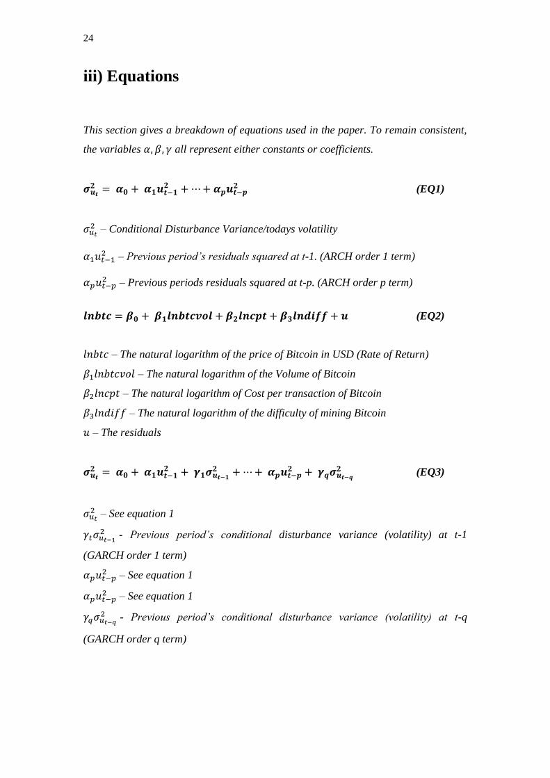
iii) Equations

This section gives a breakdown of equations used in the paper. To remain consistent,

the variables 𝛼, 𝛽, 𝛾 all represent either constants or coefficients.

𝝈𝒖𝒕𝟐 = 𝜶𝟎 + 𝜶𝟏𝒖𝒕−𝟏

𝟐 + ⋯ + 𝜶𝒑𝒖𝒕−𝒑𝟐 (EQ1)

𝜎𝑢𝑡2 – Conditional Disturbance Variance/todays volatility

𝛼1𝑢𝑡−12 – Previous period’s residuals squared at t-1. (ARCH order 1 term)

𝛼𝑝𝑢𝑡−𝑝2 – Previous periods residuals squared at t-p. (ARCH order p term)

𝒍𝒏𝒃𝒕𝒄 = 𝜷𝟎 + 𝜷𝟏𝒍𝒏𝒃𝒕𝒄𝒗𝒐𝒍 + 𝜷𝟐𝒍𝒏𝒄𝒑𝒕 + 𝜷𝟑𝒍𝒏𝒅𝒊𝒇𝒇 + 𝒖 (EQ2)

𝑙𝑛𝑏𝑡𝑐 – The natural logarithm of the price of Bitcoin in USD (Rate of Return)

𝛽1𝑙𝑛𝑏𝑡𝑐𝑣𝑜𝑙 – The natural logarithm of the Volume of Bitcoin

𝛽2𝑙𝑛𝑐𝑝𝑡 – The natural logarithm of Cost per transaction of Bitcoin

𝛽3𝑙𝑛𝑑𝑖𝑓𝑓 – The natural logarithm of the difficulty of mining Bitcoin

𝑢 – The residuals

𝝈𝒖𝒕𝟐 = 𝜶𝟎 + 𝜶𝟏𝒖𝒕−𝟏

𝟐 + 𝜸𝟏𝝈𝒖𝒕−𝟏𝟐 + ⋯ + 𝜶𝒑𝒖𝒕−𝒑

𝟐 + 𝜸𝒒𝝈𝒖𝒕−𝒒𝟐 (EQ3)

𝜎𝑢𝑡2 – See equation 1

𝛾𝑡𝜎𝑢𝑡−12 - Previous period’s conditional disturbance variance (volatility) at t-1

(GARCH order 1 term)

𝛼𝑝𝑢𝑡−𝑝2 – See equation 1

𝛼𝑝𝑢𝑡−𝑝2 – See equation 1

𝛾𝑞𝜎𝑢𝑡−𝑞2 - Previous period’s conditional disturbance variance (volatility) at t-q

(GARCH order q term)

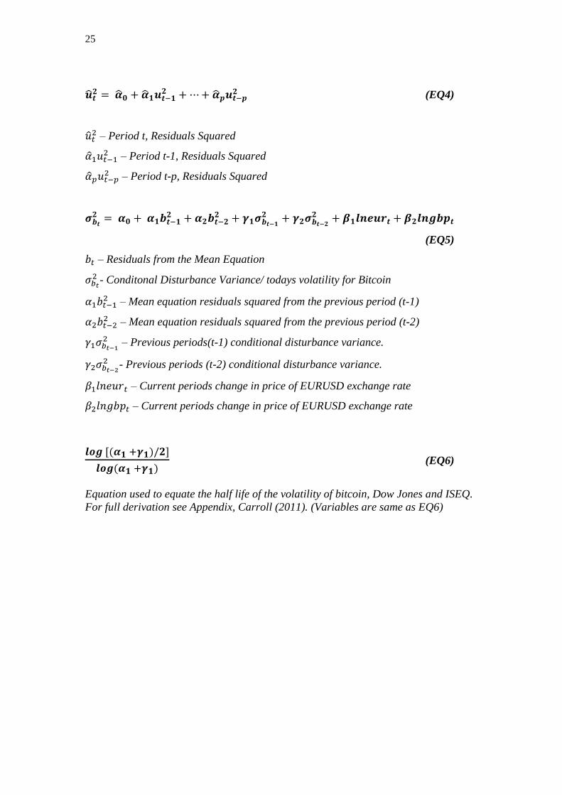
25

�̂�𝒕𝟐 = �̂�𝟎 + �̂�𝟏𝒖𝒕−𝟏

𝟐 + ⋯ + �̂�𝒑𝒖𝒕−𝒑𝟐 (EQ4)

�̂�𝑡2 – Period t, Residuals Squared

�̂�1𝑢𝑡−12 – Period t-1, Residuals Squared

�̂�𝑝𝑢𝑡−𝑝2 – Period t-p, Residuals Squared

𝝈𝒃𝒕

𝟐 = 𝜶𝟎 + 𝜶𝟏𝒃𝒕−𝟏𝟐 + 𝜶𝟐𝒃𝒕−𝟐

𝟐 + 𝜸𝟏𝝈𝒃𝒕−𝟏

𝟐 + 𝜸𝟐𝝈𝒃𝒕−𝟐

𝟐 + 𝜷𝟏𝒍𝒏𝒆𝒖𝒓𝒕 + 𝜷𝟐𝒍𝒏𝒈𝒃𝒑𝒕

(EQ5)

𝑏𝑡 – Residuals from the Mean Equation

𝜎𝑏𝑡

2 - Conditonal Disturbance Variance/ todays volatility for Bitcoin

𝛼1𝑏𝑡−12 – Mean equation residuals squared from the previous period (t-1)

𝛼2𝑏𝑡−22 – Mean equation residuals squared from the previous period (t-2)

𝛾1𝜎𝑏𝑡−1

2 – Previous periods(t-1) conditional disturbance variance.

𝛾2𝜎𝑏𝑡−2

2 - Previous periods (t-2) conditional disturbance variance.

𝛽1𝑙𝑛𝑒𝑢𝑟𝑡 – Current periods change in price of EURUSD exchange rate

𝛽2𝑙𝑛𝑔𝑏𝑝𝑡 – Current periods change in price of EURUSD exchange rate

𝒍𝒐𝒈 [(𝜶𝟏 +𝜸𝟏)/𝟐]

𝒍𝒐𝒈(𝜶𝟏 +𝜸𝟏) (EQ6)

Equation used to equate the half life of the volatility of bitcoin, Dow Jones and ISEQ.

For full derivation see Appendix, Carroll (2011). (Variables are same as EQ6)

26

7. Reference list

Alexander, C. (2008). Market risk analysis. 1st ed. Chichester, England: Wiley, p.283. Archive.today, (2006). Xak.com: Currency Strategists: Morgan Says Pound Is Euro Proxy. [online] Available at: http://archive.today/Hkb6X#selection-852.35-852.38 [Accessed 6 May. 2014]. Bagus, P. (2009). The Quality of Money. Quarterly Journal of Austrian Economics, 12(4). Bitcoin.org, (2014). How does Bitcoin work? - Bitcoin. [online] Available at: https://bitcoin.org/en/how-it-works Bitcoin.org, (n.d.). FAQ - Bitcoin. [online] Available at: https://bitcoin.org/en/faq#why-do-people-trust-bitcoin. Bollen.R (2013), Conclusions and Recommendations, The legal status of online currencies; are Bitcoins the future? Bollerlslev T (1986), Generalized Autoregressive Conditional Heteroskedasticity, Journal of Econometrics 31 Bollerslev, T. (1986). Generalized autoregressive conditional heteroskedasticity. Journal of econometrics, 31(3), pp.307--327. Carroll, T. and Collins, J. (2012). Volatility models and the ISEQ index Cont, R. (2007). Volatility clustering in financial markets: empirical facts and agent-based models. Springer, pp.289--309. Cryptonomics (2014). Is Bitcoin volatility really in decline? [online] Available at: http://cryptonomics.org/2014/01/22/is-bitcoin-volatility-really-in-decline/ [Assessed 9th May 2014] Engle, R. (1982). Autoregressive conditional heteroscedasticity with estimates of the variance of United Kingdom inflation. Econometrica: Journal of the Econometric Society, pp.987--1007. Engle, R. (2001). GARCH 101: The use of ARCH/GARCH models in applied econometrics. Journal of economic perspectives, pp.157--168. Engle, R. and Patton, A. (2001). What good is a volatility model. Quantitative finance, 1(2), pp.237--245. Fama, E. F. (1965). The behavior of stock-market prices. Journal of business, 34-105. Fergusson A (1975). When money dies. 1st ed. London: Kimber. Giller, D. (2009). Why Use the Generalized Error Distribution?. [online] Blog.gillerinvestments.com. Available at: http://blog.gillerinvestments.com/post/2009/3/19/Why-Use-the-Generalized-Error-Distribution.aspx [Accessed 7 May. 2014].

27

Hoppe (1994),The Review of Austrian Economics, Volume 7, Issue 2, pp 49-74 IMF, (n.d.). Currency Composition of Official Foreign Exchange Reserves (COFER). [online] Available at: http://www.imf.org/external/np/sta/cofer/eng/cofer.pdf. Jondeau, E., Poon, S. and Rockinger, M. (2007). Financial modeling under non-gaussian distributions. 1st ed. London: Springer, p.92. KrugenP (2011), “Golden Cyberfetters”, New York Times, “ 7 September 2011 (krugman.blogs.ny times.com/2011/09/07/golden-cyberfetters, accessed 30 April 2014) Lee S & Hansen B (1994) , Asymptotic Theory for the GARCH (1,1) Quasi-maximum Likelihood Estimator Mandelbrot, B. (1963). The Variation of Certain Speculative Prices. The Journal of Business, 36(4), pp.394-419. Nasdaq (2014), What companies accept Bitcoin ?, [online] Available at: http://www.nasdaq.com/article/what-companies-accept-bitcoin-cm323438 [Assessed 15th March 214] North.G (2013), “Bitcoins: The Second Biggest Ponzi Scheme in History”, 29 November 2013(http://www.garynorth.com/public/11828.cfm, assessed 30 April 2014) Patterson.S (2013), “Is bitcoin a viable currency?”, Foundation for Economic Education, 11 December 2013 (www.fee.org/the_freeman/detail/is-Bitcoin-a-viable-currency, assessed 30 April 2014) Quantcast (2013), Who uses Bitcoins ?, [online] Available at: https://www.quantcast.com/inside-quantcast/2013/04/who-uses-bitcoins/ [Assessed 14th April 2014] Rothbard, M. (1983). The mystery of banking. 1st ed. New York, N.Y.: Richardson & Snyder. Sciencedirect.com, (2009). On the macroeconomic causes of exchange rate volatility. [online] Available at: http://www.sciencedirect.com/science/article/pii/S0169207009000375 [Accessed 6 May. 2014]. Selgin.G (1994), On Ensuring the Acceptability of a New Fiat Money, Journal of Money, Credit and Banking, Vol. 26, No. 4, Pg 808 – 826 Simulacrum (2013), The demographics of Bitcoin(Part 1 Updated), [online] Available at: http://simulacrum.cc/2013/03/04/the-demographics-of-bitcoin-part-1-updated/ [Assessed 10th April 2014] The Economist(2011), Bits and bob[online] Available at: http://www.economist.com/blogs/babbage/2011/06/virtual-currency [Accessed 1st May 2014]

28

The Economist, (2011). Bits and bob. [online] Available at: http://www.economist.com/node/18836780 [Accessed 8 May. 2014].