The El Nino Stochastic Oscillator

Gerrit BurgersRoyal Netherlands Meteorological Institute, The Netherlands

Submitted to Journal of ClimateApril, 1997

Gerrit BurgersOceanographic Research DivisionRoyal Netherlands Meteorological Institute (KNMI)PO Box 201, 3730 AE De BiltThe Netherlands

Phone: +31 302206682fax: +31 302210407e-mail: burgers@knmi.nl

The El Nino Stochastic Oscillator

Gerrit Burgers

Royal Netherlands Meteorological Institute, The Netherlands

Submitted to Journal of Climate, April 1997

abstract

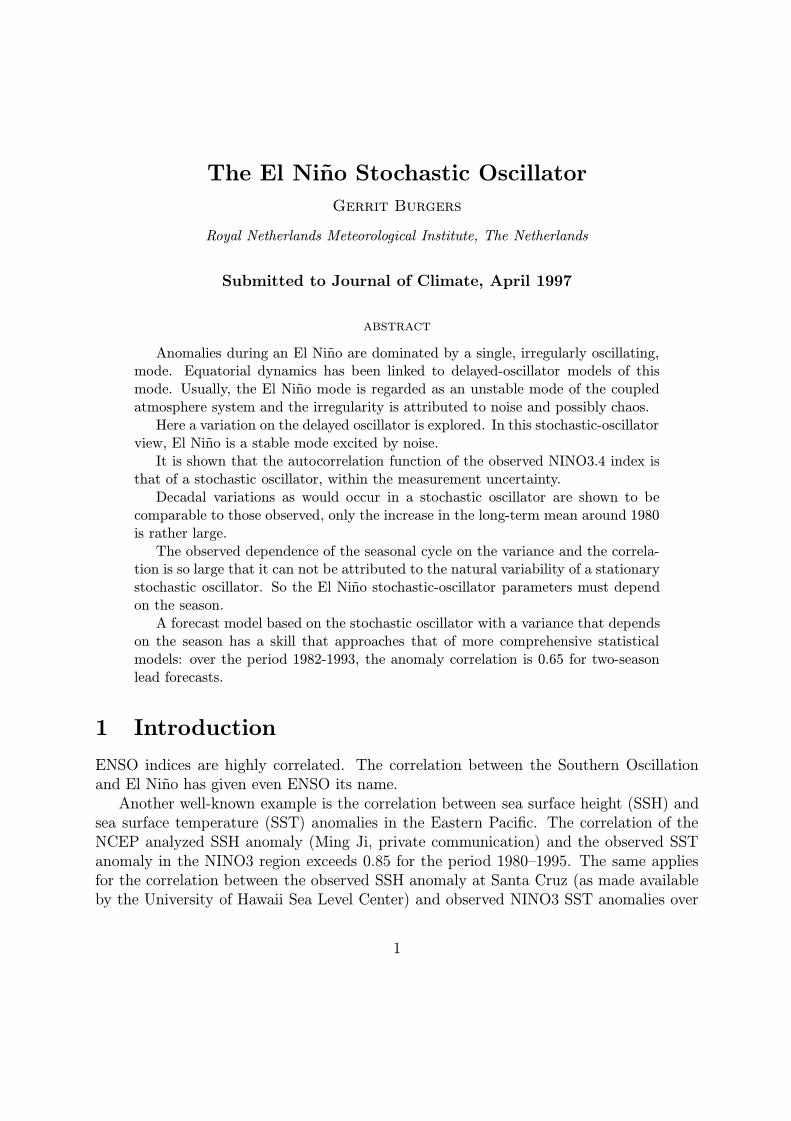
Anomalies during an El Nino are dominated by a single, irregularly oscillating,mode. Equatorial dynamics has been linked to delayed-oscillator models of thismode. Usually, the El Nino mode is regarded as an unstable mode of the coupledatmosphere system and the irregularity is attributed to noise and possibly chaos.

Here a variation on the delayed oscillator is explored. In this stochastic-oscillatorview, El Nino is a stable mode excited by noise.

It is shown that the autocorrelation function of the observed NINO3.4 index isthat of a stochastic oscillator, within the measurement uncertainty.

Decadal variations as would occur in a stochastic oscillator are shown to becomparable to those observed, only the increase in the long-term mean around 1980is rather large.

The observed dependence of the seasonal cycle on the variance and the correla-tion is so large that it can not be attributed to the natural variability of a stationarystochastic oscillator. So the El Nino stochastic-oscillator parameters must dependon the season.

A forecast model based on the stochastic oscillator with a variance that dependson the season has a skill that approaches that of more comprehensive statisticalmodels: over the period 1982-1993, the anomaly correlation is 0.65 for two-seasonlead forecasts.

1 Introduction

ENSO indices are highly correlated. The correlation between the Southern Oscillationand El Nino has given even ENSO its name.

Another well-known example is the correlation between sea surface height (SSH) andsea surface temperature (SST) anomalies in the Eastern Pacific. The correlation of theNCEP analyzed SSH anomaly (Ming Ji, private communication) and the observed SSTanomaly in the NINO3 region exceeds 0.85 for the period 1980–1995. The same appliesfor the correlation between the observed SSH anomaly at Santa Cruz (as made availableby the University of Hawaii Sea Level Center) and observed NINO3 SST anomalies over

1

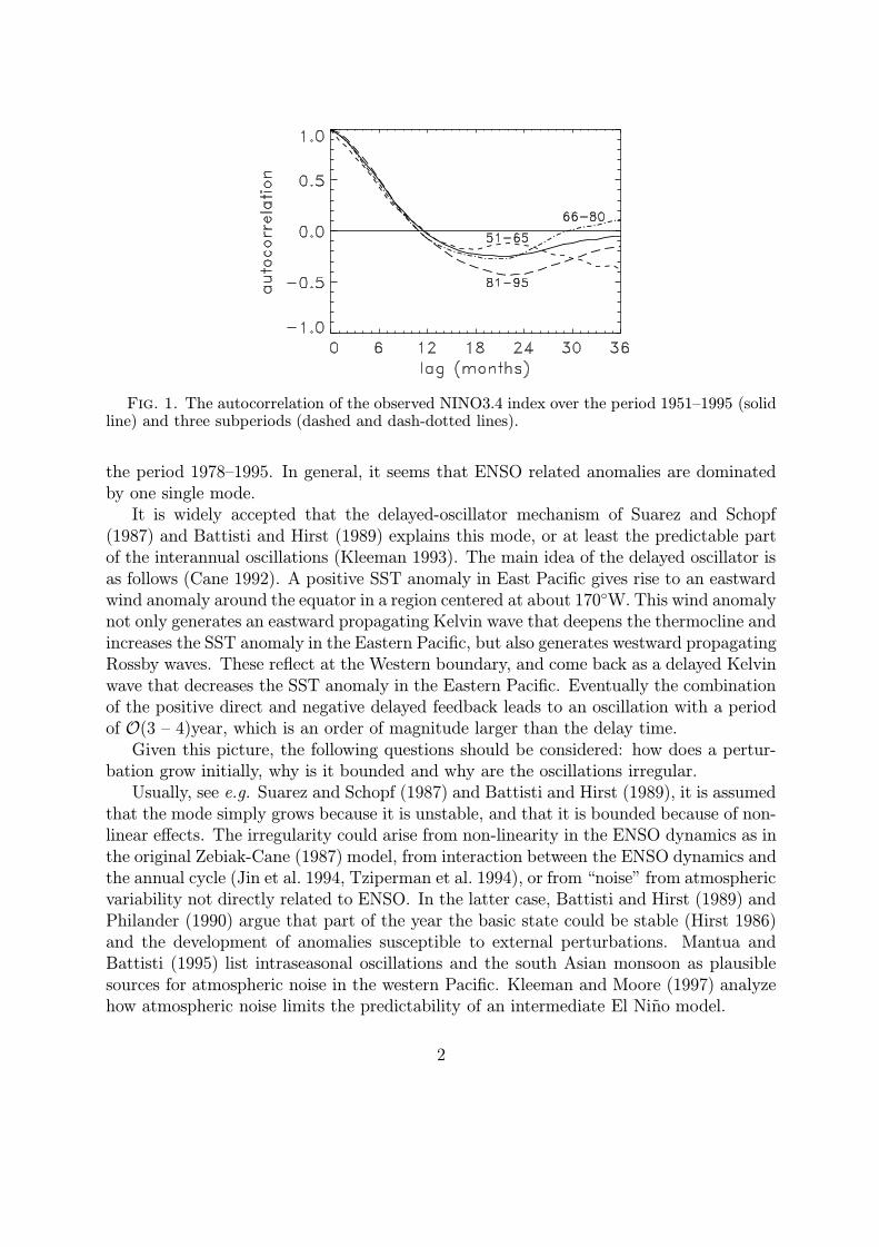
Fig. 1. The autocorrelation of the observed NINO3.4 index over the period 1951–1995 (solidline) and three subperiods (dashed and dash-dotted lines).

the period 1978–1995. In general, it seems that ENSO related anomalies are dominatedby one single mode.

It is widely accepted that the delayed-oscillator mechanism of Suarez and Schopf(1987) and Battisti and Hirst (1989) explains this mode, or at least the predictable partof the interannual oscillations (Kleeman 1993). The main idea of the delayed oscillator isas follows (Cane 1992). A positive SST anomaly in East Pacific gives rise to an eastwardwind anomaly around the equator in a region centered at about 170◦W. This wind anomalynot only generates an eastward propagating Kelvin wave that deepens the thermocline andincreases the SST anomaly in the Eastern Pacific, but also generates westward propagatingRossby waves. These reflect at the Western boundary, and come back as a delayed Kelvinwave that decreases the SST anomaly in the Eastern Pacific. Eventually the combinationof the positive direct and negative delayed feedback leads to an oscillation with a periodof O(3 – 4)year, which is an order of magnitude larger than the delay time.

Given this picture, the following questions should be considered: how does a pertur-bation grow initially, why is it bounded and why are the oscillations irregular.

Usually, see e.g. Suarez and Schopf (1987) and Battisti and Hirst (1989), it is assumedthat the mode simply grows because it is unstable, and that it is bounded because of non-linear effects. The irregularity could arise from non-linearity in the ENSO dynamics as inthe original Zebiak-Cane (1987) model, from interaction between the ENSO dynamics andthe annual cycle (Jin et al. 1994, Tziperman et al. 1994), or from “noise” from atmosphericvariability not directly related to ENSO. In the latter case, Battisti and Hirst (1989) andPhilander (1990) argue that part of the year the basic state could be stable (Hirst 1986)and the development of anomalies susceptible to external perturbations. Mantua andBattisti (1995) list intraseasonal oscillations and the south Asian monsoon as plausiblesources for atmospheric noise in the western Pacific. Kleeman and Moore (1997) analyzehow atmospheric noise limits the predictability of an intermediate El Nino model.

2

Consider now the autocorrelation function of the NINO3 or the NINO3.4 index1. Theautocorrelation function of the NINO3.4 index over the period 1951–1995 is shown inFig. 1. It is a fairly smooth function of the delay time and looks like a decaying cosinefunction. This suggests an alternative mechanism to explain the size and irregularity ofENSO.

In this explanation, the ENSO mode is stable, and noise both excites this mode andmakes it irregular.

The simplest model which exhibits such behaviour, that of a stochastic oscillator, hasan autocorrelation function that is a decaying cosine, just like observed. So I proposea stochastic-oscillator mechanism to describe ENSO. The idea is not new. Jin (1997)discusses in some detail a stochastic oscillator as one possible mechanism to excite hiscoupled recharge oscillator ENSO model. New in the present paper is that the stochas-tic oscillator is tested as a forecast model, and that the consequences of the stochasticoscillator mechanism for decadal variability are investigated.

Hasselmann (1976) introduced the concept of stochastic forcing as a source of variabil-ity in climate modelling. Most applications have dealt with the case of a red variabilityspectrum caused by a white noise forcing. Lau (1985) proposed that ENSO fluctua-tions are the result of stochastic forcing inducing transitions between multiple equilibriumstates. The idea of a stochastic oscillator is a very natural one too. It has been appliedto model variability of the thermohaline circulation (Griffies and Tziperman 1995) andto discuss decadal variability (Griffies and Bryan 1997; Munnich et al. 1997). A decadaldelayed oscillator model for exchanges between the tropics and the extratropics has beenproposed by Gu and Philander (1997). Chang, Ji and Li (1997) discuss stochasticallyexcited oscillatory modes in the context of decadal variability in the Tropical Atlanticand Jin (1997) for ENSO.

Above, the delayed-oscillator picture and the observed NINO3.4 index autocorrelationsuggested to look at a stochastic oscillator. Another motivation stems from the success ofhybrid coupled models (Balmaseda et al. 1994, Latif 1987, Barnett et al. 1993), which havestable coupled modes. Flugel and Chang (1996) and Eckert and Latif (1997) studied theimpact of an extra stochasting forcing in a HCM. The stochastic oscillator can be viewedas a representation of the main coupled mode of such a HCM with noise. Alternatively,one can arrive at the stochastic oscillator if one uses statistical techniques for signalprocessing, like fitting autoregressive-moving average (ARMA) models to timeseries, ormaking a POP or CCA analysis of observed fields. Indeed, Penland and Sardeshmukh(1995), who made an inverse modeling analysis of SST anomalies, have put forward thenotion that the El Nino system is stable and driven by white noise, although they do notpropose a system of the simple stochastic-oscillator type.

In section 2 the stochastic oscillator is formulated, and its autocorrelation function iscompared with the observed autocorrelation of the NINO3.4 index.

Simply by chance, considering a series of periods of say fifteen years, there will be fluc-tuations in properties like mean, variance and apperent autocorrelation parameters that

1The NINO3 index is the mean SST anomaly of the region 5◦S–5◦N, 150◦W–90◦W, and the NINO3.4index of the region 5◦S–5◦N, 170◦W–120◦W.

3

might account for the observed fluctuations in these parameters. This will be discussedin section 3.

In section 4 the influence of the seasonal cycle is discussed. A simple modification ofthe stationary stochastic oscillator which allows for a seasonal dependence of the varianceis introduced.

In section 5 forecasts made with the stochastic oscillator are evaluated. The simplemodel, based on the timeseries of a single variable, has a forecast skill that is comparableto that of some models actually used for ENSO predictions.

Finally, section 6 contains a discussion and the conclusion. Some technical aspects ofthe stochastical oscillator are discussed in Appendix A.

2 The stochastic oscillator model

The observed autocorrelation of the NINO3.4 index over the period 1951-1995 was shownin Fig. 1, toghether with the autocorrelations over the three 15-year long subperiods. TheNINO indices have been made available by the U.S. National Centers for Environmen-tal Prediction (NCEP), and are the result of the processing of satellite, ship and buoyobservations (Reynolds and Smith 1994).

The autocorrelation has a rather regular shape, like a damped oscillation. The differ-ences between the three fifteen year periods shown are considerable, though. This suggeststhat random fluctuations are important, and that it is probably not meaningful to extractmore than two or three parameters above the noise from a fit to this autocorrelation.

As mentioned in the Introduction, the delayed-oscillator model is about the simplestsystem ENSO can be reduced to. At the level of simplification of the delayed-oscillator,one can just as well take a regular oscillator as a model of the dynamics of the coupledsystem. The interpretation of the delayed-oscillator is of course more direct. To fitthe observed autocorrelation, some source of irregularity has to be introduced. One ofthe simplest ways to accomplish this is just adding noise. The resulting system is thestochastic oscillator.

The basic equations of the discrete stochastic oscillator can be written as follows:

xi+1 = axi − byi + ξi

yi+1 = bxi + ayi + ηi (1)

Here x and y are the variables of the two degrees of freedom of the oscillator, a and b areconstants and ξ and η are noise terms, which may be correlated. It is assumed that noisebetween different timesteps is not correlated. The constants a and b can be related to aoscillation period T = 2πω−1 and a decay time scale D = γ−1 as follows:

a+ ib = e−γ∆t eiω∆t , (2)

where ∆t is the timestep.Throughout this paper, the value of the timestep is ∆t= 1 month.

4

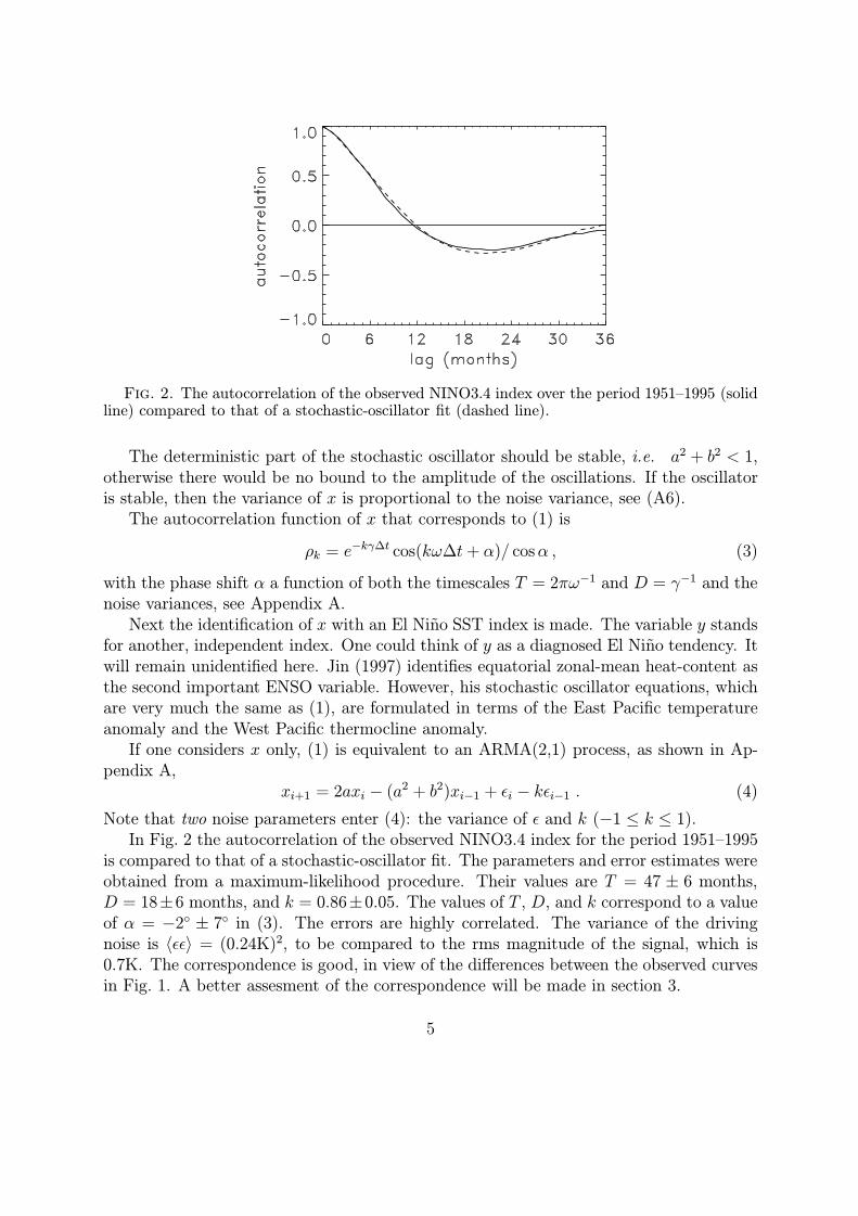
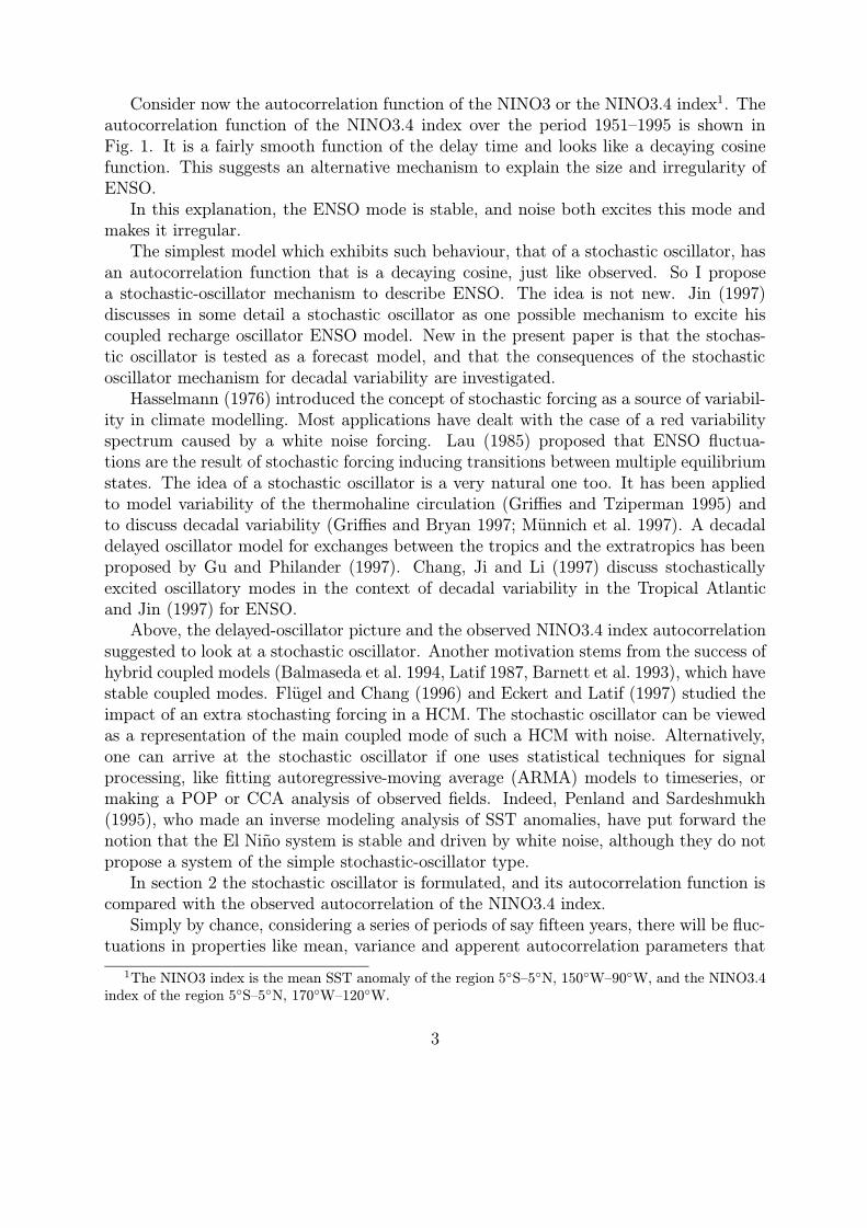
Fig. 2. The autocorrelation of the observed NINO3.4 index over the period 1951–1995 (solidline) compared to that of a stochastic-oscillator fit (dashed line).

The deterministic part of the stochastic oscillator should be stable, i.e. a2 + b2 < 1,otherwise there would be no bound to the amplitude of the oscillations. If the oscillatoris stable, then the variance of x is proportional to the noise variance, see (A6).

The autocorrelation function of x that corresponds to (1) is

ρk = e−kγ∆t cos(kω∆t+ α)/ cosα , (3)

with the phase shift α a function of both the timescales T = 2πω−1 and D = γ−1 and thenoise variances, see Appendix A.

Next the identification of x with an El Nino SST index is made. The variable y standsfor another, independent index. One could think of y as a diagnosed El Nino tendency. Itwill remain unidentified here. Jin (1997) identifies equatorial zonal-mean heat-content asthe second important ENSO variable. However, his stochastic oscillator equations, whichare very much the same as (1), are formulated in terms of the East Pacific temperatureanomaly and the West Pacific thermocline anomaly.

If one considers x only, (1) is equivalent to an ARMA(2,1) process, as shown in Ap-pendix A,

xi+1 = 2axi − (a2 + b2)xi−1 + εi − kεi−1 . (4)

Note that two noise parameters enter (4): the variance of ε and k (−1 ≤ k ≤ 1).In Fig. 2 the autocorrelation of the observed NINO3.4 index for the period 1951–1995

is compared to that of a stochastic-oscillator fit. The parameters and error estimates wereobtained from a maximum-likelihood procedure. Their values are T = 47 ± 6 months,D = 18±6 months, and k = 0.86±0.05. The values of T , D, and k correspond to a valueof α = −2◦ ± 7◦ in (3). The errors are highly correlated. The variance of the drivingnoise is 〈εε〉 = (0.24K)2, to be compared to the rms magnitude of the signal, which is0.7K. The correspondence is good, in view of the differences between the observed curvesin Fig. 1. A better assesment of the correspondence will be made in section 3.

5

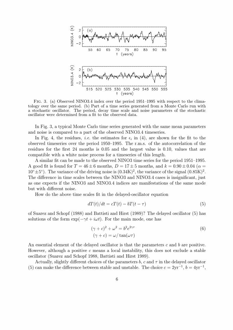
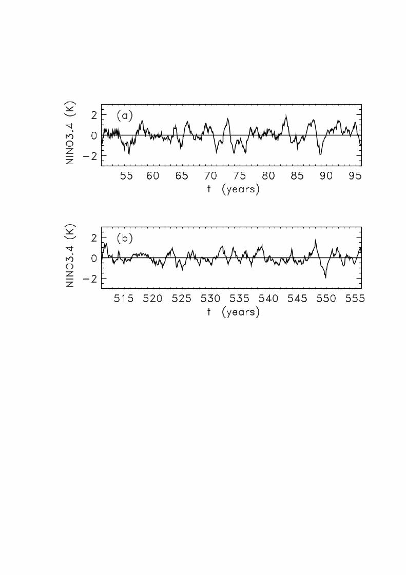
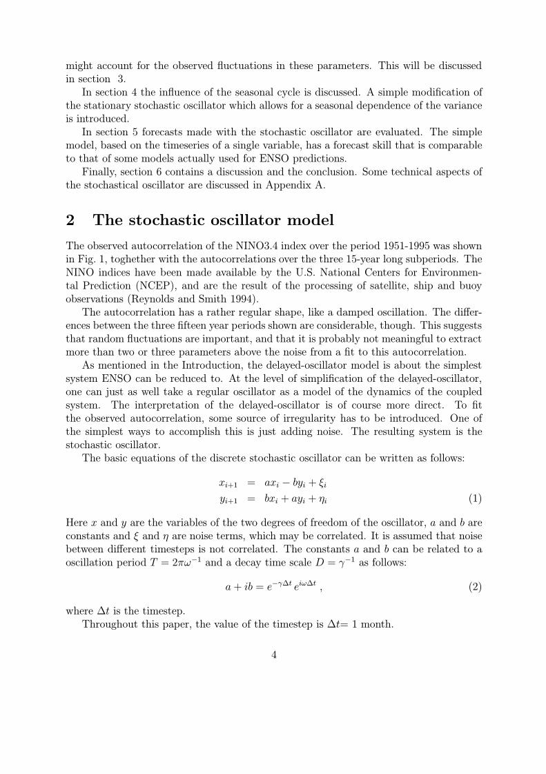
Fig. 3. (a) Observed NINO3.4 index over the period 1951–1995 with respect to the clima-tology over the same period. (b) Part of a time series generated from a Monte Carlo run witha stochastic oscillator. The period, decay time scale and noise parameters of the stochasticoscillator were determined from a fit to the observed data.

In Fig. 3, a typical Monte Carlo time series generated with the same mean parametersand noise is compared to a part of the observed NINO3.4 timeseries.

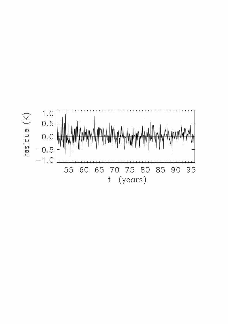
In Fig. 4, the residues, i.e. the estimates for εi in (4), are shown for the fit to theobserved timeseries over the period 1950–1995. The r.m.s. of the autocorrelation of theresidues for the first 24 months is 0.05 and the largest value is 0.10, values that arecompatible with a white noise process for a timeseries of this length.

A similar fit can be made to the observed NINO3 time series for the period 1951–1995.A good fit is found for T = 46± 6 months, D = 17± 5 months, and k = 0.90± 0.04 (α =10◦±5◦). The variance of the driving noise is (0.34K)2, the variance of the signal (0.85K)2.The difference in time scales between the NINO3 and NINO3.4 cases is insignificant, justas one expects if the NINO3 and NINO3.4 indices are manifestations of the same modebut with different noise.

How do the above time scales fit in the delayed-oscillator equation

dT (t)/dt = cT (t)− bT (t− τ) (5)

of Suarez and Schopf (1988) and Battisti and Hirst (1989)? The delayed oscillator (5) hassolutions of the form exp(−γt+ iωt). For the main mode, one has

(γ + c)2 + ω2 = b2e2γτ (6)

(γ + c) = ω/ tan(ωτ)

An essential element of the delayed oscillator is that the parameters c and b are positive.However, although a positive c means a local instability, this does not exclude a stableoscillator (Suarez and Schopf 1988, Battisti and Hirst 1989).

Actually, slightly different choices of the parameters b, c and τ in the delayed oscillator(5) can make the difference between stable and unstable. The choice c = 2yr−1, b = 4yr−1,

6

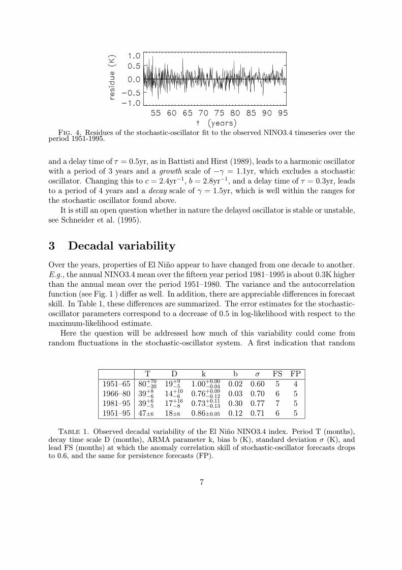
Fig. 4. Residues of the stochastic-oscillator fit to the observed NINO3.4 timeseries over theperiod 1951-1995.

and a delay time of τ = 0.5yr, as in Battisti and Hirst (1989), leads to a harmonic oscillatorwith a period of 3 years and a growth scale of −γ = 1.1yr, which excludes a stochasticoscillator. Changing this to c = 2.4yr−1, b = 2.8yr−1, and a delay time of τ = 0.3yr, leadsto a period of 4 years and a decay scale of γ = 1.5yr, which is well within the ranges forthe stochastic oscillator found above.

It is still an open question whether in nature the delayed oscillator is stable or unstable,see Schneider et al. (1995).

3 Decadal variability

Over the years, properties of El Nino appear to have changed from one decade to another.E.g., the annual NINO3.4 mean over the fifteen year period 1981–1995 is about 0.3K higherthan the annual mean over the period 1951–1980. The variance and the autocorrelationfunction (see Fig. 1 ) differ as well. In addition, there are appreciable differences in forecastskill. In Table 1, these differences are summarized. The error estimates for the stochastic-oscillator parameters correspond to a decrease of 0.5 in log-likelihood with respect to themaximum-likelihood estimate.

Here the question will be addressed how much of this variability could come fromrandom fluctuations in the stochastic-oscillator system. A first indication that random

T D k b σ FS FP1951–65 80+70

−20 19+9−5 1.00+0.00

−0.04 0.02 0.60 5 41966–80 39+8

−6 14+10−6 0.76+0.09

−0.12 0.03 0.70 6 51981–95 39+6

−5 17+16−8 0.73+0.11

−0.13 0.30 0.77 7 51951–95 47±6 18±6 0.86±0.05 0.12 0.71 6 5

Table 1. Observed decadal variability of the El Nino NINO3.4 index. Period T (months),decay time scale D (months), ARMA parameter k, bias b (K), standard deviation σ (K), andlead FS (months) at which the anomaly correlation skill of stochastic-oscillator forecasts dropsto 0.6, and the same for persistence forecasts (FP).

7

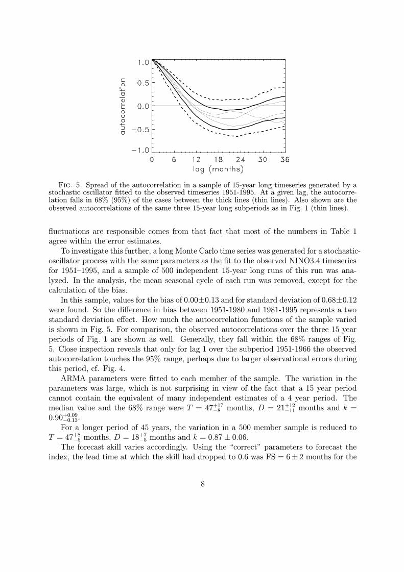
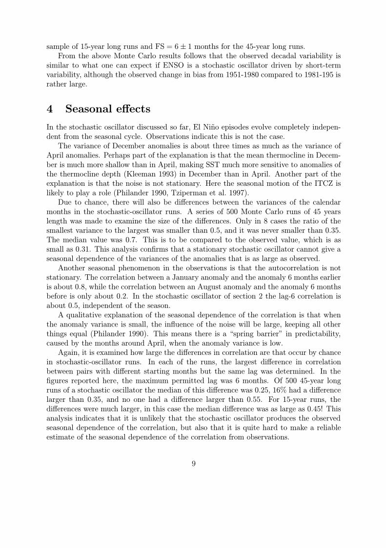
Fig. 5. Spread of the autocorrelation in a sample of 15-year long timeseries generated by astochastic oscillator fitted to the observed timeseries 1951-1995. At a given lag, the autocorre-lation falls in 68% (95%) of the cases between the thick lines (thin lines). Also shown are theobserved autocorrelations of the same three 15-year long subperiods as in Fig. 1 (thin lines).

fluctuations are responsible comes from that fact that most of the numbers in Table 1agree within the error estimates.

To investigate this further, a long Monte Carlo time series was generated for a stochastic-oscillator process with the same parameters as the fit to the observed NINO3.4 timeseriesfor 1951–1995, and a sample of 500 independent 15-year long runs of this run was ana-lyzed. In the analysis, the mean seasonal cycle of each run was removed, except for thecalculation of the bias.

In this sample, values for the bias of 0.00±0.13 and for standard deviation of 0.68±0.12were found. So the difference in bias between 1951-1980 and 1981-1995 represents a twostandard deviation effect. How much the autocorrelation functions of the sample variedis shown in Fig. 5. For comparison, the observed autocorrelations over the three 15 yearperiods of Fig. 1 are shown as well. Generally, they fall within the 68% ranges of Fig.5. Close inspection reveals that only for lag 1 over the subperiod 1951-1966 the observedautocorrelation touches the 95% range, perhaps due to larger observational errors duringthis period, cf. Fig. 4.

ARMA parameters were fitted to each member of the sample. The variation in theparameters was large, which is not surprising in view of the fact that a 15 year periodcannot contain the equivalent of many independent estimates of a 4 year period. Themedian value and the 68% range were T = 47+17

−8 months, D = 21+12−11 months and k =

0.90+0.09−0.13.For a longer period of 45 years, the variation in a 500 member sample is reduced to

T = 47+8−5 months, D = 18+7

−5 months and k = 0.87± 0.06.The forecast skill varies accordingly. Using the “correct” parameters to forecast the

index, the lead time at which the skill had dropped to 0.6 was FS = 6± 2 months for the

8

sample of 15-year long runs and FS = 6± 1 months for the 45-year long runs.From the above Monte Carlo results follows that the observed decadal variability is

similar to what one can expect if ENSO is a stochastic oscillator driven by short-termvariability, although the observed change in bias from 1951-1980 compared to 1981-195 israther large.

4 Seasonal effects

In the stochastic oscillator discussed so far, El Nino episodes evolve completely indepen-dent from the seasonal cycle. Observations indicate this is not the case.

The variance of December anomalies is about three times as much as the variance ofApril anomalies. Perhaps part of the explanation is that the mean thermocline in Decem-ber is much more shallow than in April, making SST much more sensitive to anomalies ofthe thermocline depth (Kleeman 1993) in December than in April. Another part of theexplanation is that the noise is not stationary. Here the seasonal motion of the ITCZ islikely to play a role (Philander 1990, Tziperman et al. 1997).

Due to chance, there will also be differences between the variances of the calendarmonths in the stochastic-oscillator runs. A series of 500 Monte Carlo runs of 45 yearslength was made to examine the size of the differences. Only in 8 cases the ratio of thesmallest variance to the largest was smaller than 0.5, and it was never smaller than 0.35.The median value was 0.7. This is to be compared to the observed value, which is assmall as 0.31. This analysis confirms that a stationary stochastic oscillator cannot give aseasonal dependence of the variances of the anomalies that is as large as observed.

Another seasonal phenomenon in the observations is that the autocorrelation is notstationary. The correlation between a January anomaly and the anomaly 6 months earlieris about 0.8, while the correlation between an August anomaly and the anomaly 6 monthsbefore is only about 0.2. In the stochastic oscillator of section 2 the lag-6 correlation isabout 0.5, independent of the season.

A qualitative explanation of the seasonal dependence of the correlation is that whenthe anomaly variance is small, the influence of the noise will be large, keeping all otherthings equal (Philander 1990). This means there is a “spring barrier” in predictability,caused by the months around April, when the anomaly variance is low.

Again, it is examined how large the differences in correlation are that occur by chancein stochastic-oscillator runs. In each of the runs, the largest difference in correlationbetween pairs with different starting months but the same lag was determined. In thefigures reported here, the maximum permitted lag was 6 months. Of 500 45-year longruns of a stochastic oscillator the median of this difference was 0.25, 16% had a differencelarger than 0.35, and no one had a difference larger than 0.55. For 15-year runs, thedifferences were much larger, in this case the median difference was as large as 0.45! Thisanalysis indicates that it is unlikely that the stochastic oscillator produces the observedseasonal dependence of the correlation, but also that it is quite hard to make a reliableestimate of the seasonal dependence of the correlation from observations.

9

The above results show that the stationary stochastic oscillator model of section 2 isincomplete because it lacks seasonal dependence in variance and correlation.

In principle, the extension is clear: make all parameters dependent on the season, andrepeat the analysis to get the best fit to the observed seasonal dependence. This will notbe attempted here. Instead, the following simple trick is used. The analysis of section 2 isredone on data scaled to unit variance month-by-month. Stochastic-oscillator parametersfrom fits to these standarized anomalies are given in Table 2. The values are similar tothose for fits to the full NINO3.4 anomalies in Table 1.

A stochastic oscillator model of the standarized anomalies is equivalent to a seasonalstochastic oscillator which is obtained by multiplying the r.h.s. of (1) by a factor thatdepends on the calendar month, the products of these factors being unity. This makes thatfor the NINO3.4 seasonal stochastic oscillator the deterministic part grows in boreal falland decays relatively fast in early spring, giving rise to the observed seasonal dependenceof the variance. Also, it implies that the noise is larger if the deterministic part favoursgrowth, thus neglecting the seasaonal dependence of the correlation.

Although the above modification leaves the correlation unchanged and independent ofthe season, it is a great improvement of the covariance. In Fig. 6. the observed covarianceas a function of lag and final month is compared to that of a stationary stochastic-oscillatorfit and to that of a fit of a stochastic oscillator with seasonal variance. Note that althoughtheir correlations are almost identical and independent of the season, the second and thethird panel look less similar than the first and the third.

Actually, the anomaly correlation of the seasonal stochastic-oscillator forecast for thefull (destandarized) anomalies is somewhat larger than the skills of Table 2. This is be-cause high-variance months are generally better predictable than low-variance monthsin terms of anomaly correlation, due the observed seasonal dependence of the correla-tions. This applies to persistence skill as well: forecasts based on persistent standarizedanomalies have more skill than forecasts based on persistent anomalies.

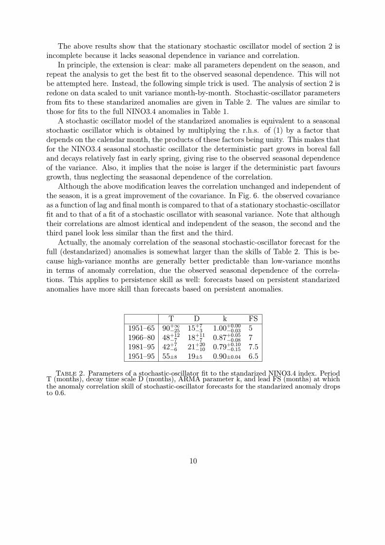
T D k FS1951–65 90+∞

−25 15+7−3 1.00+0.00

−0.03 51966–80 48+12

−7 18+11−7 0.87+0.05

−0.08 71981–95 42+7

−6 21+20−10 0.79+0.10

−0.15 7.51951–95 55±8 19±5 0.90±0.04 6.5

Table 2. Parameters of a stochastic-oscillator fit to the standarized NINO3.4 index. PeriodT (months), decay time scale D (months), ARMA parameter k, and lead FS (months) at whichthe anomaly correlation skill of stochastic-oscillator forecasts for the standarized anomaly dropsto 0.6.

10

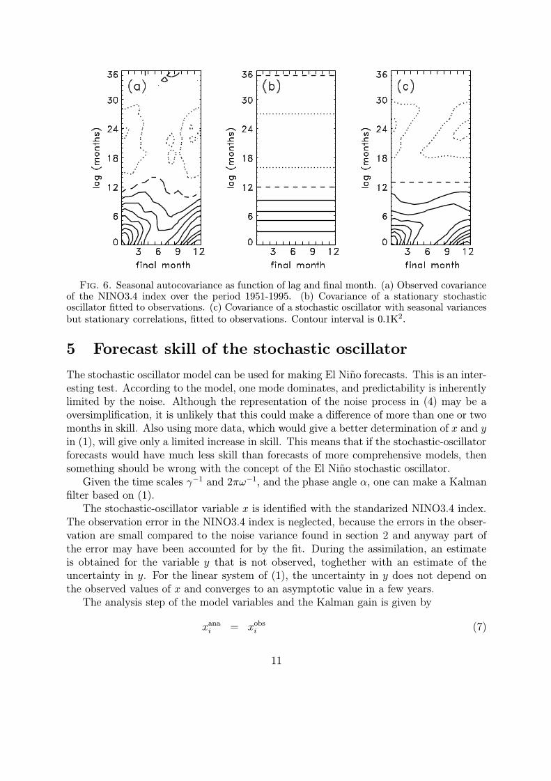
Fig. 6. Seasonal autocovariance as function of lag and final month. (a) Observed covarianceof the NINO3.4 index over the period 1951-1995. (b) Covariance of a stationary stochasticoscillator fitted to observations. (c) Covariance of a stochastic oscillator with seasonal variancesbut stationary correlations, fitted to observations. Contour interval is 0.1K2.

5 Forecast skill of the stochastic oscillator

The stochastic oscillator model can be used for making El Nino forecasts. This is an inter-esting test. According to the model, one mode dominates, and predictability is inherentlylimited by the noise. Although the representation of the noise process in (4) may be aoversimplification, it is unlikely that this could make a difference of more than one or twomonths in skill. Also using more data, which would give a better determination of x and yin (1), will give only a limited increase in skill. This means that if the stochastic-oscillatorforecasts would have much less skill than forecasts of more comprehensive models, thensomething should be wrong with the concept of the El Nino stochastic oscillator.

Given the time scales γ−1 and 2πω−1, and the phase angle α, one can make a Kalmanfilter based on (1).

The stochastic-oscillator variable x is identified with the standarized NINO3.4 index.The observation error in the NINO3.4 index is neglected, because the errors in the obser-vation are small compared to the noise variance found in section 2 and anyway part ofthe error may have been accounted for by the fit. During the assimilation, an estimateis obtained for the variable y that is not observed, toghether with an estimate of theuncertainty in y. For the linear system of (1), the uncertainty in y does not depend onthe observed values of x and converges to an asymptotic value in a few years.

The analysis step of the model variables and the Kalman gain is given by

xanai = xobs

i (7)

11

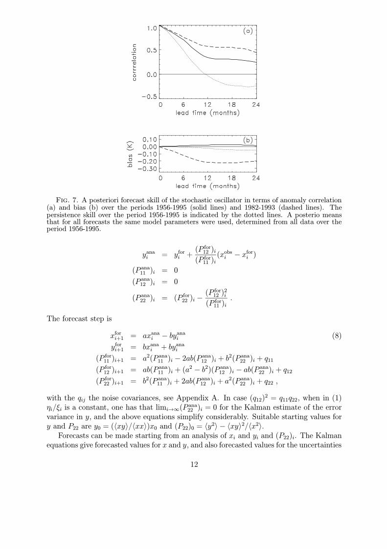
Fig. 7. A posteriori forecast skill of the stochastic oscillator in terms of anomaly correlation(a) and bias (b) over the periods 1956-1995 (solid lines) and 1982-1993 (dashed lines). Thepersistence skill over the period 1956-1995 is indicated by the dotted lines. A posterio meansthat for all forecasts the same model parameters were used, determined from all data over theperiod 1956-1995.

yanai = yfor

i +(P for

12 )i(P for

11 )i(xobs

i − xfori )

(P ana11 )i = 0

(P ana12 )i = 0

(P ana22 )i = (P for

22 )i −(P for

12 )2i

(P for11 )i

.

The forecast step is

xfori+1 = axana

i − byanai (8)

yfori+1 = bxana

i + byanai

(P for11 )i+1 = a2(P ana

11 )i − 2ab(P ana12 )i + b2(P ana

22 )i + q11

(P for12 )i+1 = ab(P ana

11 )i + (a2 − b2)(P ana12 )i − ab(P

ana22 )i + q12

(P for22 )i+1 = b2(P ana

11 )i + 2ab(P ana12 )i + a2(P ana

22 )i + q22 ,

with the qij the noise covariances, see Appendix A. In case (q12)2 = q11q22, when in (1)ηi/ξi is a constant, one has that limi→∞(P ana

22 )i = 0 for the Kalman estimate of the errorvariance in y, and the above equations simplify considerably. Suitable starting values fory and P22 are y0 = (〈xy〉/〈xx〉)x0 and (P22)0 = 〈y2〉 − 〈xy〉2/〈x2〉.

Forecasts can be made starting from an analysis of xi and yi and (P22)i. The Kalmanequations give forecasted values for x and y, and also forecasted values for the uncertainties

12

in x and y. An alternative is making an ensemble of forecast runs, using (1) with differentnoise for each ensemble member. Finally, the forecasted values for x are destandarized toget the full anomalies.

The Kalman filter was tried on the NINO3.4 index, because the NINO3.4 index ismore persistent and easier to predict than the NINO3 index.

In a first experiment, forecasts over the period 1956–1995 were made with a modelfitted to the same period. Because the model parameters were determined using thetimeseries over the full period, these are not really forecasts in the strict sense that nofuture information is used, and the skill is overestimated substantially. In principle, thesame applies to persistence forecasts based on a climatology calculated over the full periodtoo, but in that case the effect is only marginal.

The skill as measured by the anomaly correlation and the bias of these “a posteriori”forecasts is shown in Fig. 7. The correlation drops to about 0.6 after 7.5 months. Thisamounts to a gain of 2.5 month over simple persistence skill and of 1.5 month over “stan-darized persistence” skill (not shown). Also shown in Fig. 7 is that the skill was higherover the subperiod 1982–1993 than over 1956-1995. However, for longer lead times, thebias over this subperiod is large. This is because for longer lead times, the stochastic-oscillator forecasts relax to the climatology of the full period instead of to the subperiodmean.

In another experiment, quasi-operational forecasts were made for the period 1976–1995. The model parameters (biases, variances, stochastic-oscillator parameters) for eachforecast were determined using only data from 1956 to the starting month of the forecast.The skill of these quasi-operational forecasts is shown in Fig. 8. Also shown in Fig. 8 isthe skill of the quasi-operational forecasts over the subperiod 1982-1993. As one sees, thequasi-operational skill is somewhat lower than the a posterio skill. Over 1982-1993, theanomaly correlation drops to 0.6 after 8.5 months, and the bias is about −0.3K for longerlead times.

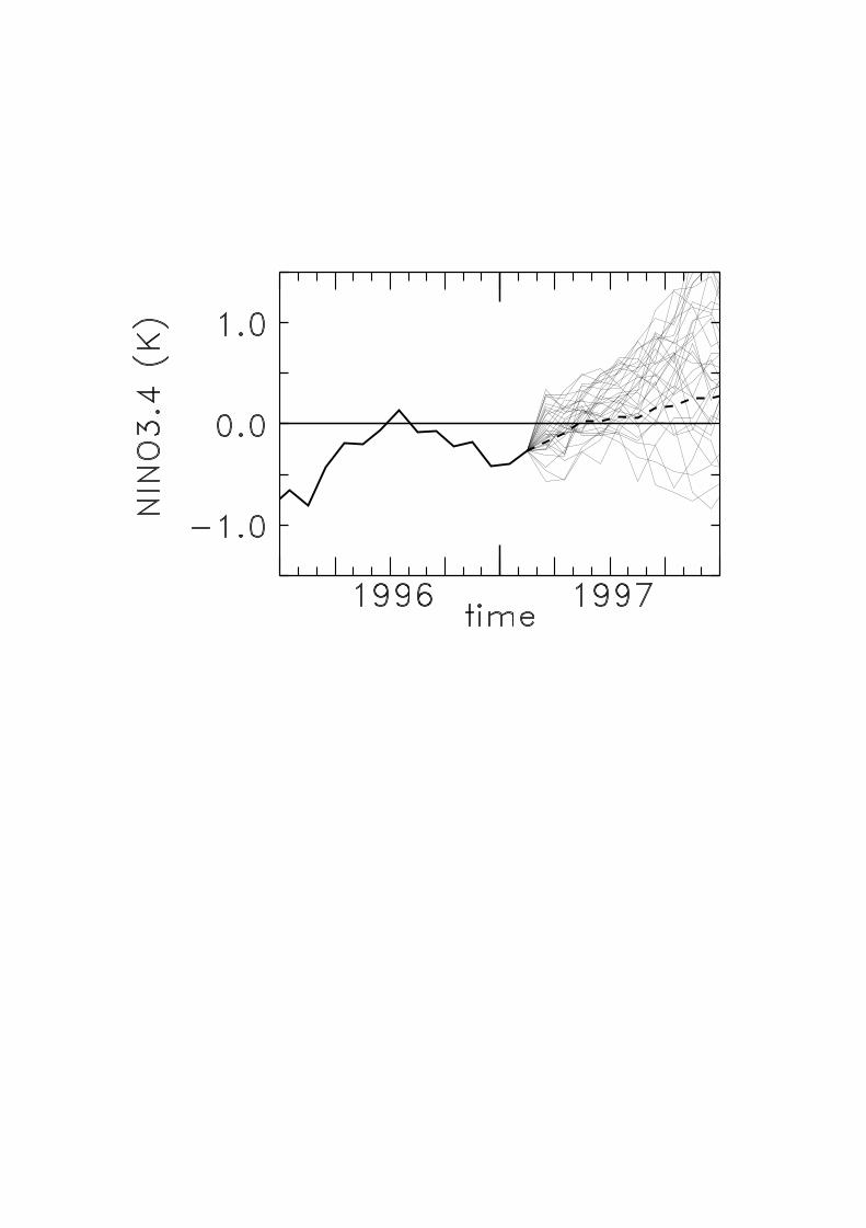
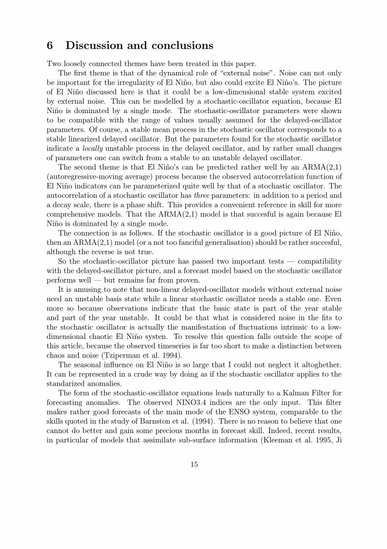
The reader may check the forecast of Fig. 9, which was made just before this paperwas submitted. It shows the Kalman Filter forecast from February 1997, toghether witha 32-member ensemble forecast.

A comparison of two-season lead forecasts by Barnston et al. (1994) concentratedon the relatively well-predictable sub-period 1982–1993. The anomaly correlation of aquasi-operational two-season lead forecast as defined by Barnston et al., which roughlycorresponds to the anomaly correlation at eight months as presented here, is 0.65 for thequasi-operational forecasts. This is comparable to the skill of the models considered inBarnston et al. and significantly better than the anomaly-correlation skill of persistence,which is 0.33 for the period considered.

The above results indicate that the stochastic oscillator is quite capable of succesfulpredicting the main ENSO mode.

13

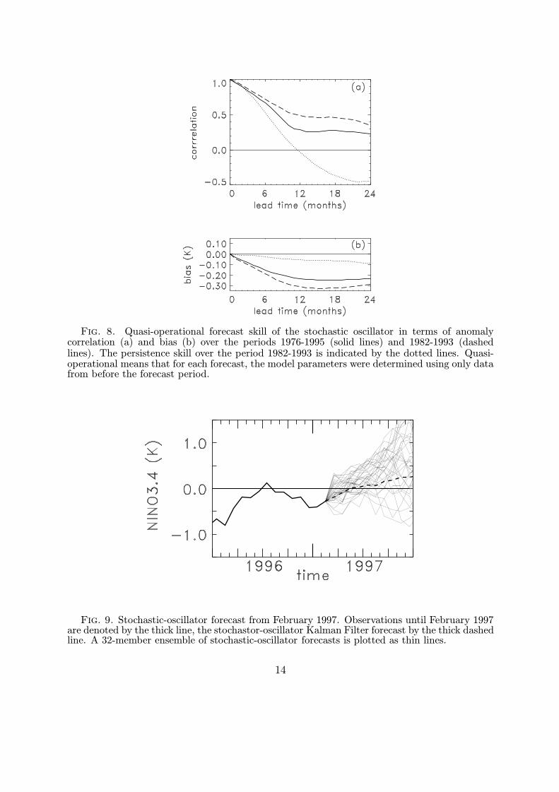
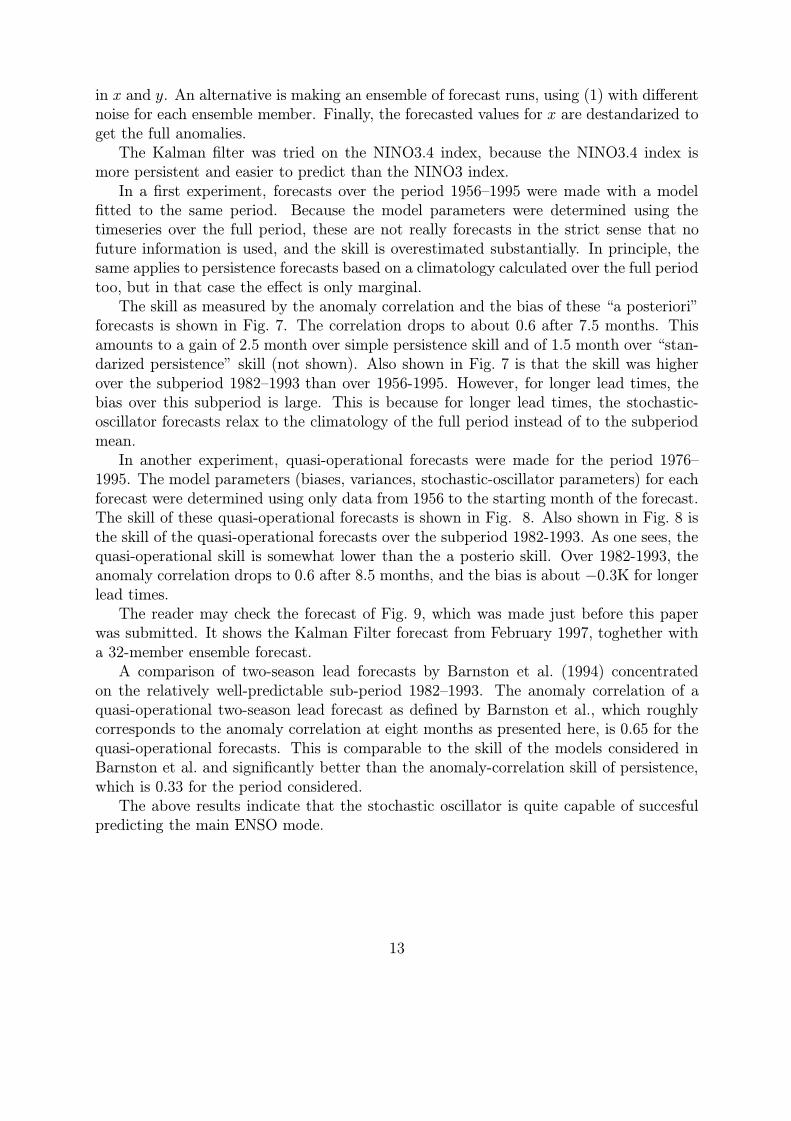
Fig. 8. Quasi-operational forecast skill of the stochastic oscillator in terms of anomalycorrelation (a) and bias (b) over the periods 1976-1995 (solid lines) and 1982-1993 (dashedlines). The persistence skill over the period 1982-1993 is indicated by the dotted lines. Quasi-operational means that for each forecast, the model parameters were determined using only datafrom before the forecast period.

Fig. 9. Stochastic-oscillator forecast from February 1997. Observations until February 1997are denoted by the thick line, the stochastor-oscillator Kalman Filter forecast by the thick dashedline. A 32-member ensemble of stochastic-oscillator forecasts is plotted as thin lines.

14

6 Discussion and conclusions

Two loosely connected themes have been treated in this paper.The first theme is that of the dynamical role of “external noise”. Noise can not only

be important for the irregularity of El Nino, but also could excite El Nino’s. The pictureof El Nino discussed here is that it could be a low-dimensional stable system excitedby external noise. This can be modelled by a stochastic-oscillator equation, because ElNino is dominated by a single mode. The stochastic-oscillator parameters were shownto be compatible with the range of values usually assumed for the delayed-oscillatorparameters. Of course, a stable mean process in the stochastic oscillator corresponds to astable linearized delayed oscillator. But the parameters found for the stochastic oscillatorindicate a locally unstable process in the delayed oscillator, and by rather small changesof parameters one can switch from a stable to an unstable delayed oscillator.

The second theme is that El Nino’s can be predicted rather well by an ARMA(2,1)(autoregressive-moving average) process because the observed autocorrelation function ofEl Nino indicators can be parameterized quite well by that of a stochastic oscillator. Theautocorrelation of a stochastic oscillator has three parameters: in addition to a period anda decay scale, there is a phase shift. This provides a convenient reference in skill for morecomprehensive models. That the ARMA(2,1) model is that succesful is again because ElNino is dominated by a single mode.

The connection is as follows. If the stochastic oscillator is a good picture of El Nino,then an ARMA(2,1) model (or a not too fanciful generalisation) should be rather succesful,although the reverse is not true.

So the stochastic-oscillator picture has passed two important tests — compatibilitywith the delayed-oscillator picture, and a forecast model based on the stochastic oscillatorperforms well — but remains far from proven.

It is amusing to note that non-linear delayed-oscillator models without external noiseneed an unstable basis state while a linear stochastic oscillator needs a stable one. Evenmore so because observations indicate that the basic state is part of the year stableand part of the year unstable. It could be that what is considered noise in the fits tothe stochastic oscillator is actually the manifestation of fluctuations intrinsic to a low-dimensional chaotic El Nino systen. To resolve this question falls outside the scope ofthis article, because the observed timeseries is far too short to make a distinction betweenchaos and noise (Tziperman et al. 1994).

The seasonal influence on El Nino is so large that I could not neglect it altoghether.It can be represented in a crude way by doing as if the stochastic oscillator applies to thestandarized anomalies.

The form of the stochastic-oscillator equations leads naturally to a Kalman Filter forforecasting anomalies. The observed NINO3.4 indices are the only input. This filtermakes rather good forecasts of the main mode of the ENSO system, comparable to theskills quoted in the study of Barnston et al. (1994). There is no reason to believe that onecannot do better and gain some precious months in forecast skill. Indeed, recent results,in particular of models that assimilate sub-surface information (Kleeman et al. 1995, Ji

15

et al. 1996), seem to point to an improvement in model skill in recent years.Even within the context of the stochastic oscillator, improvement in forecast skill could

come from more comprehensive models. Seasonality might be represented better, data-assimilation might give an better estimate of the two deterministic degrees of freedomof the system, and the noise might be better represented and partly predictable. Also,going slightly beyond the stochastic-oscillator picture, it might very well be that the noisevariance could be dependent on El Nino.

If models as the stochastic oscillator are tuned on relatively short testing periods,forecast skill may be overestimated considerably.

The stochastic oscillator exhibits substantial decadal variability. This applies not onlyto the apperent mean state and that some periods are more active than others. It alsoapplies to predictability: even with a “perfect” model, during some periods forecasts aremuch more succesful than during others.

Acknowledgements I thank Geert Jan van Oldenborgh and Gerbrand Komen for manydiscussions and Adri Buishand for providing me with a maximum-likelihood algorithmfor determining the parameters of an ARMA process.

Appendix A Properties of the stochastic oscillator

The simplest form of the stochastic oscillator is the complex Langevin equation

z = −cz + ζ(t) (A1)

for a complex variable z, with a complex constant c and a noise term ζ . The noise ζ is notspecified as a given function of time, but it assumed that its average 〈ζ〉 = 0, that ζ(t) isdistributed according a Gaussian law and that its second moment 〈ζ(t)ζ(t− τ)〉 is given.The autocorrelation of ζ should go to zero at times much smaller than the mean timescale | c |−1, for a meaningful separation of mean and stochastic processes to be possible.(A1) has the formal solution

z = z0e−ct + e−ct

∫ t

0dτ ecτζ(τ) . (A2)

A clear account of the theory of the real Langevin equation can be found in Balescu(1975).

In this paper, the discretized form of (A1) is considered:

xi+1 = axi − byi + ξi

yi+1 = bxi + ayi + ηi (A3)

for two real variables x and y, real constants a and b and noise terms ξi and ηi. From(A3) follows the following equation in terms of x alone:

xi+1 = 2axi − (a2 + b2)xi−1 + ξi − aξi−1 − bηi−1 . (A4)

16

In the following, the timescales γ−1 and 2πω−1 will be used. They are defined by

a+ ib = e−γ∆t eiω∆t , (A5)

with ∆t the timestep.Next, the assumption is made that the noise between different timesteps in (A3) is

not correlated. Going back to a complex variable and using formal solutions analoguousto (A2), the following expressions for the variances of the variables x and y in term of thevariances of the noise can be obtained:

〈x2〉 =1

2

(q11 + q22)

1− e−2γ∆t+

1

2

(1− 2e−2γ∆t cos(2ω∆t)) (q11 − q22)

1− 2e−2γ∆t cos(2ω∆t) + e−4γ∆t(A6)

−e−2γ∆t sin(2ω∆t) q12

1− 2e−2γ∆t cos(2ω∆t) + e−4γ∆t

〈y2〉 =q11 + q22

1− e−2γ∆t− 〈x2〉

〈xy〉 =1

2

e−2γ∆t sin(2ω∆t) (q11 − q22)

1− 2e−2γ∆t cos(2ω∆t) + e−4γ∆t+

(1− 2e−2γ∆t cos(2ω∆t)) q12

1− 2e−2γ∆t cos(2ω∆t) + e−4γ∆t,

with

q11 = 〈ξiξi〉 (A7)

q22 = 〈ηiηi〉

q12 = 〈ξiηi〉 .

The autocorrelation function of x, ρk = 〈xi+kxi〉/〈xixi〉 is given by

ρk = e−kγ∆t cos(kω∆t+ α)/ cosα , (A8)

tanα = 〈xy〉/〈x2〉 . (A9)

So in addition to the mean-process timescales γ−1 and ω−1 there is a third parameter inthe autocorrelation function, the phase shift α. The phase shift depends both on the meanand the noise parameters. In the special case that q12 = 0 and q11 = q22, one has 〈xy〉 = 0and α = 0. In the limit ω → 0, ω tanα→ −r, one has ρk → exp(−γk∆t)(1 + rk∆t).

If one would make a POP (Hasselmann 1988) analysis of x and y, or of observed fieldsdominated by a mode linearly related to x and y, then the leading POP mode will havethe stochastic-oscillator period and decay time scale.

Looking only at one variable, the stochastic oscillator reduces to what in term ofautoregressive modelling is called an ARMA(2,1) (autoregressive-moving average) process:

xi+1 = 2axi − (a2 + b2)xi−1 + εi − kεi−1 , (A10)

where the correspondence between the ARMA noise variance

q00 = 〈εiεi〉 (A11)

17

and the noise parameters q11, q22 and q12 is given by

(1 + k2)q00 = (1 + a2)q11 + b2q22 + 2abq12 (A12)

kq00 = aq11 + bq12 .

Note that k and 1/k are equivalent. To one value of k corresponds a curve of combinationsof q22/q11 and q12/q11 which have the same variance and autocorrelation for x but differin the variance and autocorrelation of y.

The power spectrum which corresponds to the autocorrelation function of (A8) is inthe limit ∆t→ 0 that of a broad peak with a red tail:

S(ω′) =1

2π

{γ − tanα(ω′ − ω)

(ω′ − ω)2 + γ2+γ + tanα(ω′ + ω)

(ω′ + ω)2 + γ2

}. (A13)

18

references

Balescu, R., 1975: Equilibrium and nonequilibrium statistical mechanics, J. Wiley & Sons, 742pp.Balmaseda, M.A., D.L.T. Anderson, and M.K. Davey, 1994: ENSO prediction using a dynamical

ocean model coupled to statistical atmospheres. Tellus, 46A, 497–511.Barnett, T.P., M. Latif, M. Flugel, S. Pazan, and W. White, 1993: ENSO and ENSO-related

predictability: Part I - Prediction of equatorial Pacific sea surface temperature with ahybrid coupled ocean-atmosphere model. J. Climate, 6, 1545–1566.

Barnston, G.B., H.M. van den Dool, S.E. Zebiak, T.P. Barnett, Ming Ji, D.R. Rodenhuis, M.A.Cane, A. Leetmaa, N.E. Graham, C.F. Ropelewski, V.E. Kousky, E.A. O’Lenic, andR.E. Livezey, 1994: Long-lead seasonal forecasts – where do we stand? Bull. Am. Met.Soc., 75, 2097–2114.

Battisti, D.S., and A.C. Hirst, 1989: Interannual variability in a tropical atmosphere-oceanmodel: Influence of the basic state, ocean geometry and nonlinearity. J. Atmos. Sci.,46, 1687–1712.

Cane, M.A., 1992: Tropical Pacific ENSO models: ENSO as a mode of the coupled system. In:Climate System Modeling, K.E. Trenberth ed., Cambridge University Press, p583–614.

Chang, P., L. Ji, and H. Li, 1997: A decadal climate variation in the tropical Atlantic Oceanfrom thermodynamic air-sea interactions. Nature, 385, 516–518.

Eckert, C. and M. Latif, 1997: Predictability of a stochastically forced hybrid coupled model ofEl Nino. J. Clim., (accepted).

Flugel, M. and P. Chang, 1996: Impact of dynamical and stochastic processes on the predictabil-ity of ENSO. Geophys. Res. Let., 23, 2089-2092.

Griffies, S.M., and K. Bryan, 1997: Predictability of North Atlantic multidecadal climate vari-ability. Science, 275, 181–184.

, and E. Tziperman, 1995: A linear thermohaline oscillator driven by stochastic atmo-spheric forcing. J. Clim., 8, 2440–2453.

Gu D., and S.G.H. Philander, 1997: Interdecadal climate fluctuations that depend on exchangesbetween the tropics and extratropics. Science, 275, 805–807.

Hasselmann, K., 1976: Stochastic climate models. Part 1. Theory. Tellus, 18, 473–485., 1988: PIP’s and POP’s: The reduction of complex dynamical systems using principal

interaction and oscillation patterns. J. Geophys. Res., 93, 11015–11021.Hirst, A.C., 1986: Unstable and damped equatorial modes in simple coupled ocean-atmosphere

models. J. Atmos. Sci., 43, 606–630.Ji, M., A. Leetmaa, and V.E. Kousky, 1996: Coupled model predictions of ENSO during the

1980s and the 1990s at the National Centers for Environmental Prediction. J. Clim.,9, 3105–3120.

Jin, F.-F., D. Neelin, and M. Ghil, 1994: ENSO on the devil’s staircase. Science, 263,70–72., 1997: An equatorial ocean recharge paradigm for ENSO. Part I: Conceptual model. J.

Atmos. Sci., 54, 811–829.Kleeman, R., 1993: On the dependence of the hindcast skill on ocean thermodynamics in a

coupled ocean-atmosphere model. J. Clim., 6, 2012–2033., Moore and N.R. Smith, 1995: Assimiliation of sub-surface thermal data into an inter-

mediate tropical coupled ocean-atmosphere model. Mon. Wea. Rev., 123, 3103–3113., and , 1997: A theory for the limitation of ENSO predictability due to stochastic

atmospheric transients. J. Atmos. Sci., 54, 753–767.

19

Latif, M., 1987: Tropical ocean circulation experiments. J. Phys. Oceanogr., 17, 246–263.Lau, K.M., 1985: Elements of a stochastic-dynamical theory of the long-term variability of the

El Nino/Southern Oscillation. J. Atmos. Sci., 42, 1552–1558.Mantua, N.J., and D.S. Battisti 1995: Aperiodic variability in the Zebiak-Cane coupled ocean-

atmosphere model: air-sea interactions in the western equatorial Pacific. J. Clim., 8,2897–2927.

Munnich, M., M. Latif, S. Venzke, and E. Maier-Reimer, 1997: Decadal oscillations in a simplecoupled model. submitted to J. Phys. Oceanogr.

Penland, C., and P.D. Sardeshmukh, 1995: The optimal growth of tropical sea surface temper-ature anomalies. J. Clim., 8, 1999–2024.

Philander, S.G.H., 1990: El Nino, La Nina and the Southern Oscillation. Academic Press,293pp.

Reynolds, R.W., and T.M. Smith, 1994: Improved global sea surface temperature analyses usingoptimum interpolation. J. Clim., 7, 929–948.

Schneider E.K., B. Huang, and J. Shukla, 1995: Ocean wave dynamics and El Nino. J. Clim.,8, 2415–2439.

Tziperman, E., L. Stone, M.A. Cane, and H. Jarosh, 1994: El Nino chaos: Overlapping of reso-nances between the seasonal cycle and the Pacific ocean-atmospere oscillator. Science,263,72–74.

, Zebiak and M.A. Cane, 1997: Mechanisms of seasonal-Enso interaction. J. Atmos. Sci.,54, 61–71.

Zebiak, S.E., and M.A. Cane, 1987: A model El Nino-Southern Oscillation. Mon. Wea. Rev.,

115, 2262–2278.

20