Embed Size (px)
Citation preview
The Effects of Weather on Crime
James Horrocks
Department of Economics and Finance; University of Canterbury
Email: [email protected]
Ph: +64 21 778 710
Andrea Kutinova Menclova
Department of Economics and Finance; University of Canterbury
Email: [email protected]
Ph: +64 3 364 2823
Abstract
This paper uses daily data from 43 districts across New Zealand from 2000 to 2008 and employs
panel econometric techniques to investigate the effect of weather on crime. Temperature and
precipitation are found to have a significant effect on the number of violent crimes recorded and
temperature also affects the number of property crimes recorded. Studies of this nature are
important for the allocation of police resources.
As an extension, the common belief that the Nor’wester wind causes ‘disorderly’ behavior is
empirically investigated. Data on violent crime from three Canterbury police districts is used. The
Nor’wester is found to be statistically insignificant in determining the number of violent crimes
in Canterbury.
JEL Code: K42
Keywords: Property crime, Violent crime, Temperature, Precipitation
Acknowledgments: We would like to thank Bob Reed, Gregory Breetzke and participants at the
University of Canterbury Economics and Finance seminar and the Australian School of Business
National Honours Colloquium for very helpful comments. We are also indebted to the New
Zealand Police (Obert Cinco in particular) and NIWA for their data.

1
1. Introduction
Criminal activity and the factors driving it have received a lot of attention. One factor that is
believed to affect criminal activity is weather. A small body of literature empirically investigates
this relationship and mostly supports the conclusion that weather has a causal effect on criminal
activity. This paper investigates whether this relationship holds in New Zealand. Incorporating
weather into the dynamics of criminal behavior potentially provides important explanatory power
for models of criminal behavior. In addition, weather could be used as an instrumental variable in
analyses of the effects of crime on a number of variables such as property prices, quality of life
indices, economic growth, and so on. Furthermore, weather could act as a direct predictor of
criminal activity. This would be a valuable tool for police in their efforts to allocate resources.
This paper employs panel econometric techniques on daily crime and weather data from New
Zealand from 2000 to 2008. Two broad categories of crime are analyzed: property crime and
violent crime. Temperature and precipitation are used as measures of weather. The relationship
between each of the crime variables and each of the weather variables is investigated. Evidence is
found to suggest that weather has a significant effect on criminal activity.
As an extension, the effect of the North-westerly wind, which is often thought to induce
‘disorderly’ behavior, on violent crime in Canterbury is measured.
2. Theoretical Framework
The supply of criminal offences depends on the individual-specific costs and benefits of the
crime as well as individual-specific preferences and circumstances (Becker 1968). A crime will
2
be committed if the expected utility of committing a crime exceeds the expected costs (including
the opportunity costs, i.e., the expected utility of using the same amount of time and resources
elsewhere). For example, as the probability of being caught increases, the expected cost of
committing an offence increases, thereby decreasing the number of offences committed.
Similarly, if the expected punishment for an offence increases, the expected cost of committing
an offence increases, thereby decreasing the number of offences committed. Several studies
provide empirical evidence for these assertions (Sjoquist 1973). Other important determinants of
criminal activity include the potential income derived from criminal activity, moral attitudes
towards criminal behavior, risk aversion, and the opportunity set outside of criminal activity.
Weather may have an effect on the probability of being caught committing a crime as well as on
several other determinants of criminal behavior.
2.1 Violent Crime
Previous literature emphasizes the psychological impacts of weather and the resulting changes in
the propensity to commit a violent crime. For example, the Negative Affect Escape (NAE) model
stipulates that aggression increases with temperature because of increases in irritation and
discomfort, but only up to a certain point. At this point, the relationship changes to being
negative as the discomfort increases to a level where the motivation to escape uncomfortable
situations outweighs the motivation to be aggressive (Bell 1992). Thus, there is an ‘inverse-U-
shaped’ relationship between temperature and aggression. As aggression increases/decreases, the
expected utility of crime which releases that aggression also increases/decreases.
The General Affect (GA) model suggests that higher temperatures facilitate affective aggression
(Cohn and Rotton 2000a). That is, higher temperatures facilitate aggression that has its primary

3
purpose in injuring another person. The Routine Activity (RA) theory stipulates that a criminal
event requires three elements: a suitable target, a motivated offender, and the absence of capable
guardians against crime (Felson 1987; Cohn and Rotton 2000a). Relating this to weather, ‘better’
weather conditions are likely to increase the likelihood of a suitable target occurring, thus
increasing the expected utility of crime. For example, better weather will increase mobility and
social interaction as more people leave their homes thereby presenting more opportunities for
violent crime to occur. However, better weather is also likely to increase the presence of capable
guardians, increasing the probability of being caught and thus the expected costs of crime. If
more people are interacting, then there will be more capable guardians (e.g., companions or
bystanders) to prevent a crime. As a result, ‘worse’ weather may increase violence when people
do come in contact due to the lack of capable guardians. An example of this latter effect is
domestic violence. Regarding the third necessary element, motivation to commit a violent crime
may be related to temperature (as stipulated by the NAE and GA models). Thus, the overall
impact of weather on violent crime will depend on the magnitudes of the effects on all of the
three elements. For example, if temperature increases, will the increase in capable guardians (i.e.,
the increase in expected costs) counter the increase in suitable targets and motivation (i.e., the
increase in expected utility)? The RA theory is ambiguous on this point and the answer is
essentially an empirical matter.
2.2 Property Crime
Weather is likely to have an impact on social mobility. If the weather is ‘fine’, people are less
likely to be at home (Schmallager 1997). People may be more likely to go out in the evening or
go away for the weekend. The RA theory described above illustrates how this might impact on
criminal activity through the likelihood of encountering a suitable target, a motivated offender,

4
and the absence of capable guardians against crime. First, in ‘fine’ weather, it is less likely that
people will be in their homes, therefore decreasing the probability of a capable guardian being
present. This decreases the probability of being caught, thereby decreasing the expected costs and
increasing the number of property crime offences, ceteris paribus.
Second, if more homes are unoccupied, potential burglars will have a greater selection of suitable
targets. This increases the expected utility of committing a property crime as the most suitable
target can be chosen. For example, if all houses on a street are unoccupied, the burglar can
choose the most expensive house on the street, thereby increasing the expected monetary benefits
of a burglary.
Third, criminals may be less motivated to commit crimes during ‘bad’ weather. For example,
precipitation may discourage a criminal from undertaking a burglary because of the discomfort of
being outside in bad weather (and the associated expected costs). In addition, bad weather could
make transporting stolen goods, in particular electronic equipment, more difficult. Thus, overall,
we may expect ‘fine’ weather to be associated with more property crime.
2.3 Effect of Weather on Policing
It is possible that the police incorporate weather as a decision variable when deciding on the level
and intensity of policing. First, police departments may have already observed the relationship
between weather and crime and adjusted police presence accordingly. If the police presence is
consistently higher in finer weather, we would expect this to result in fewer crimes occurring as
criminals acknowledge the increased probability of being caught. This would introduce a
downward bias to the relationship between weather and crime observed in the data, making the

5
results of this study conservative (i.e., representing a lower bound of the true effect of weather on
crime, ceteris paribus). Second, effort levels of police officers may change depending on weather.
For example, if it is raining, police may not decide to do a foot patrol. The temperament of police
officers may also be affected by weather. In line with the NAE model, increased temperatures
may increase police aggression resulting in more arrests. It is important to note, however, that the
crime data used in this study consist of recorded crimes and so a police officer does not
necessarily have to witness the crime or apprehend the offender for it to be recorded. The issue of
variation in policing is a small but noteworthy limitation of our study.
3. Previous Findings
Several studies have been conducted internationally on the effects of weather on criminal
activity. The weather variables used and crimes measured vary across studies.
3.1 Violent Crime
Using weekly data from 116 jurisdictions in the U.S. from 1995 to 2001, Jacob, Lefgren, and
Moretti (2006) find that a 10°F increase in average weekly temperature is associated with a 5%
increase in violent crime. For precipitation, they find that a 1 inch increase in average weekly
precipitation is associated with a 10% reduction in violent crime. Using monthly data from
England and Wales, Field (1992) finds that temperature is positively and significantly correlated
with violent crime, sexual offences, and criminal damage. Precipitation provides no explanatory
power and is insignificant for all dependent variables. Cohn and Rotton (2000b) use data on
complaints about disorderly behavior from Minnesota over two years and find that temperature is
significantly correlated with the number of complaints. Their evidence supports the existence of a
6
curvilinear relationship, with the number of complaints increasing with temperatures up to 70ºF
and then exhibiting a negative relationship at temperatures above this point.
Cohn and Rotton (2000c) test for a curvilinear relationship between violence and temperature.
Their data consists of calls for service relating to aggravated assault over a two year period in
Dallas, Texas. When analyzing the relationship between temperature and violent crime over three
hour time periods, the authors find a curvilinear pattern, with temperature positively correlated
with calls up to 85ºF and negatively correlated thereafter. Interestingly for the purposes of this
study, the relationship is not as prominent when the data is aggregated into 24 hour time periods.
To summarize, the literature is largely consistent with the hypothesis that violent crime is
strongly correlated with temperature. In addition, there is evidence of an inverse-U-shaped
relationship between temperature and violent crime. The literature is ambiguous about the effect
of precipitation on violent crime.
3.2 Property Crime
Jacob, Lefgren, and Moretti (2006) find that a 10°F increase in the average weekly temperature is
correlated with a 3% reduction in property crime. Their results indicate that precipitation is
insignificant. Field (1992) finds that burglary, theft and robbery are all positively and
significantly correlated with temperature. Precipitation is insignificant in his results. Since
monthly data is used, the paper does not provide evidence on the effects of brief weather shocks.
Cohn and Rotton (2000a) analyze theft, burglary and robbery in Minneapolis over two years
using calls for service to measure criminal activity. They find that theft is negatively correlated

7
with precipitation and temperature and that both burglary and robbery are positively correlated
with precipitation and temperature.
To summarize, the literature is ambiguous about the effects of temperature and precipitation on
property crime.
4. Data
Daily data on recorded crime was obtained from the New Zealand Police. It covers 43 districts in
New Zealand from 1st January 2000 to 31st December 2008 and several crime categories are
available (Table 1).
From the raw data, violent and property crime variables were constructed by aggregating
different categories, as illustrated below. This aggregation largely removed zero values.
Violent Crime = Violence + Property Damage + Property AbuseProperty Crime = Theft + Burglary
‘Property Damage’ and ‘Property Abuse’ were categorized as violent crimes because they
constitute violence against property. Other categories were excluded from the main specification
because there was no theoretical justification for their inclusion. For example, fraud is unlikely to
be related to weather. In addition, most of the existing literature does not include these categories
and so excluding them makes our results more comparable.
A crime is recorded upon the report of an incident if that incident is deemed to be an offence and
there is no evidence to the contrary. In the majority of cases, violent crimes are reported on the

8
day of the crime; however, this could be an issue for some categories of violent crime. For
example, ‘Property Abuse’ such as vandalism may be reported days after the actual incident
occurred (for example, when the property owners return from holidays). Delayed reporting is a
more serious issue for property crime, as crimes are less likely to be reported immediately after
the crime has occurred. This represents a limitation of our study but an attempt is made to address
this issue by employing several lags of the weather variables.
Daily weather data was obtained from the National Institute of Water and Atmospheric Research
(NIWA) from 1st January 2000 to 31st December 2008. Weather variables collected were
maximum and minimum daily temperature (in °C) and total precipitation (in millimeters).
For each of the district/day crime observations, a corresponding weather observation had to be
found. This was done by matching police districts to the nearest weather station(s). While there
are many weather stations in New Zealand, finding the appropriate data was complicated by the
fact that weather stations often have incomplete (missing) records or do not measure either
temperature or precipitation. Another complicating issue is the treatment of large police districts.
For example, Rural Otago has a large geographic area with population concentrated in
Queenstown, which is located in the mountains, and Oamaru, which is located on the coast. As
expected, an inspection of temperature and precipitation variables for these areas revealed large
differences in weather conditions. While imperfect, our method for constructing weather
variables for areas such as Rural Otago was to take weighted averages based on population
estimates obtained at the small town level from Statistics New Zealand. So, for example, the
weather variables for Rural Otago were created by weighting Queenstown and Oamaru weather
conditions by the corresponding population estimates. This is similar to the method used by

9
Jacob, Lefgren, and Moretti (2006) in their treatment of county-level weather variables. In our
study, this method was used for 11 of the 43 police districts.
A further issue was that due to the proximity of some police districts, the same weather data had
to be used for more than one police district. This was only a problem for the 8 police districts
within Auckland. Weather data was missing for less than 1% of the days covered in the sample.
Annual population data was collected as a control. Data was sourced from Statistics New
Zealand. In some regressions, observations are weighted by population. This is done in order to
give a greater weight to observations that affect more people and thus to make the results
nationally representative. The regression results are robust to the use of population weights,
presumably largely because police districts are defined so that population is evenly dispersed.
Quarterly unemployment data was sourced from the Household Labour Force Survey (HLFS).
The data available is aggregated across 12 regions in New Zealand which means that some police
districts had to be linked with the same unemployment data. The regional unemployment rate
was used as a control in recognition of the fact that unemployment has previously been found to
be a determinant of crime in New Zealand (Papps and Winkelmann 2000).
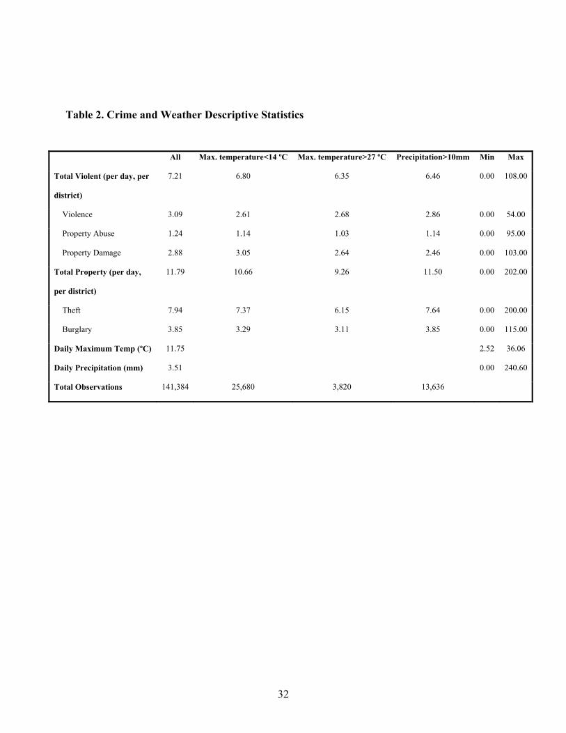
5. Descriptive Statistics
The average number of violent crimes per day per district is 7.21 and the average number of
property crimes is 11.79 (Table 2). On ‘cold days’ when the maximum temperature is less than
14ºC (57ºF), representing the coolest quintile of days, the average numbers of violent and

10
property crimes are lower than the overall means. On ‘very hot’ days when the maximum
temperature is greater than 27ºC (80ºF), the temperature that other studies have identified as a
turning point (Cohn 1990), the average numbers of violent and property crimes are also lower
than the overall mean. This is consistent with the inverse-U-shaped relationship discussed above.
On days with more than 10 millimeters (0.04 inches) of precipitation (three times the daily
average precipitation in the sample), the average number of violent crimes per district is 6.46
which is significantly lower than the sample average of 7.21. The average number of property
crimes per district is 11.50 on days with more than 10 millimeters of precipitation, which is
slightly lower than the sample average of 11.79. The maximum precipitation in our sample (241
mm; 0.95 inches) occurred in the Bay of Plenty in May 2005 during heavy flooding. The
maximum temperature (36ºC; 97ºF) was recorded in mid-south Canterbury in January 2004.
6. Methods and Results
6.1 Temperature and Violent Crime
Ordinary least squares (OLS) was used to estimate the following base specification:
2, 0 1 , 2 , 3 , ,
,
,
,
tempmax tempmax
violent offences in district on day tempmax maximum temperature in district on day
a set of controls
vd t d t d t d t d t
vd t
d t
d t
O controlswhere
O d td t
controls
β β β β ε= + + + +
===
The set of controls includes annual district population, region-specific quarterly unemployment
rate, day of the week dummy variables, an interaction term between city districts and the
weekend, month dummy variables, year dummy variables, district dummy variables, and a linear
time trend for each district. The above specification – specification (1) – is our preferred

11
specification for its intuitive appeal, simplicity, as well as its goodness-of-fit (R2=0.43).
However, as shown below, the coefficients on the temperature variables remain robust to
different alternative specifications. The results of specification (1) are presented in the first
column of Table 3. Robust standard errors are used in all specifications to correct for possible
heteroskedasticity.
The results in specification (1) - and in all other specifications - suggest that temperature has an
effect on the number of violent crimes recorded. The daily maximum temperature coefficient is
positive and significant as expected, and the coefficient on daily maximum temperature squared is
negative and significant, consistent with the proposed inverse-U-shaped relationship.
It is crucial to note that by including district and month dummies in our regressions, we are only
estimating the effects of unexpected (i.e., not given by geography and season) weather changes.
Thus, we may be underestimating the full effects of weather on crime. Unfortunately, the
alternative approach of omitting district and month dummies will produce biased estimates of the
effects of weather/climate on crime if some other factors (e.g., school holidays or immigration to
Auckland) are correlated with both of these variables. Therefore, we prefer our fixed effects
specification but note that caution is needed when deriving policy recommendations from our
findings. In particular, we emphasize that in allocating its resources, police should use
information on both district and seasonal characteristics (e.g., January in Auckland) and current
weather conditions (from short-term weather forecast) into account.
Specification (2) weights observations by annual district population, giving greater weight to
observations that affect more people. Specification (3) adds three lags of the dependent variable

12
(i.e., violent crime) to specification (2). Note that although the first and second lags are highly
significant, the effect of temperature on violent crime remains robust. Specification (4) adds
precipitation and an interaction term between temperature and precipitation as explanatory
variables to specification (3). The coefficient on precipitation is negative and significant as
expected. The interaction term is very small and insignificant which indicates that the effects of
temperature and precipitation are separate from each other. Specification (5) uses the crime rate
calculated as crimes per 100,000 people as the dependent variable with the same controls as
specification (1), excluding population. Specification (6) uses the Tobit procedure with censoring
at zero with the same controls as specification (1). The dependent variable had a value of zero in
2.5% of the sample and so the Tobit procedure was used to address any bias that may have
occurred using OLS. The coefficient estimates for temperature and temperature squared are
almost identical to the OLS estimates suggesting that no serious bias occurs when using OLS.
Specification (7) uses the average temperature of the preceding seven days as an explanatory
variable. The coefficient is small and insignificant indicating that sudden deviations from the
average temperature rather than simply warmer periods are important in determining crime.
Specification (8) allows each district to have a non-linear time trend to account for the fact that
crimes within each district may evolve differently over time. An interaction between district and
year dummy variables was used to achieve this. This specification did not alter the observed
effect of temperature on violent crime. Similarly, each month was allowed to have a district-
specific effect by interacting each district with each month. The relationship between temperature
and violent crime was unaffected by this specification (results available on request). As an
additional robustness check, specification (1) was run without temperature as an explanatory
variable. This produced an AIC value of 777,510 compared with an AIC value of 767,953 when

13
the temperature controls are included. This suggests that temperature adds explanatory power to
the specification.
Coefficients on most of the controls used (available on request) have the expected sign. As
expected, Friday and Saturday have higher levels of crime than Mondays. This result also
suggests that violent crimes are recorded when they occur; more crimes are expected on the
weekend and this is when more crimes are recorded. Population is positive and significant.
Unemployment does not have a statistically significant impact which is contrary to previous
findings in New Zealand (Papps and Winkelmann 2000). A potential source of this difference is
that Papps and Winkelmann used annual data whereas this study uses daily data: unemployment
is more likely to affect the propensity to commit crimes over a much longer time period, rather
than explaining day to day variation in crime. The coefficients on the weekend*city interaction
terms are positive and significant. This can be explained by high transitory population over the
weekend in cities relative to other districts and by increased social activity. The city districts used
were Auckland Central City, Hamilton, Wellington, Christchurch and Dunedin. The month
dummy variables produced some interesting results; with April to July having the lowest number
of violent crimes and November the highest number of crimes relative to January. A joint
coefficient test on the eleven month dummy variables produced an F-statistic of 87.42;
confirming a strong seasonal component of crime. The year dummy variables suggest that violent
crime was decreasing in the period from 2000 to 2005 and then increasing slightly in 2005 to
2008.
What specifically do our results imply about the effects of regional temperature changes on
violent crime? As an example, take consecutive Wednesdays in Counties-Manukau South in July

14
2004. These days were chosen because precipitation was zero on both days and all other controls
such as the day of the week, month, year, the unemployment rate, population and district are held
constant. This enables us to isolate the effect of an increase in temperature. The temperature on
the first Wednesday was 14.2ºC (57.6ºF) and on the second Wednesday 17.2ºC (63.0ºF). Our
model predicts an increase in the number of violent crimes by 2.2% (from 7.20 to 7.36) due to
this change in temperature (the actual number of violent crimes on both these days was 5).
Figure 1 illustrates the general effect of temperature on the total number of violent crimes implied
by our empirical models. The turning point occurs at 27ºC (80ºF – similar to Cohn 1990; Cohn
and Rotton 2000b and 2000c), indicating that violent crime increases with temperature up to that
point but then begins to decrease. To further examine this relationship, total violent crime was
regressed on the maximum temperature for days when the maximum temperature was lower than
27ºC and for days when the maximum temperature was higher than 27ºC (available on request).
On days when the maximum temperature is lower than 27ºC, maximum temperature has a
positive and significant effect. On days when temperature is greater than 27ºC, maximum
temperature has a negative but insignificant coefficient. These findings are consistent with the
curvilinear relationship estimated in specification (1), although the insignificance of the
maximum temperature variable at temperatures greater than 27ºC also allows for a zero effect of
temperature on crime – consistent with a positive but diminishing (in the limit to zero) marginal
effect of temperature on violent crime. Alternatively, the insignificance of the temperature
variable on ‘very hot’ days could be due to a small sample size (3,820 observations).

15
Care is required when interpreting the above results. Firstly, the coefficient on temperature
indicates the effect of relative (compared to other districts) temperature changes. Seasonal effects
are accounted for by the month dummy variables and any national time trend by the year dummy
variables. Since year to year changes are accounted for, no inference can be made about national,
long run changes to the average temperature. So, for example, we cannot conclude that global
warming would increase the number of violent crimes committed. Furthermore, we note that out-
of-sample predictions should not be made based on our results. For example, our results do not
apply to temperature changes at extremely low or extremely high temperatures not observed in
New Zealand.
Specification (1) was used to estimate the relationship between temperature and each of the three
subcategories of violent crime: ‘Violence’, ‘Property Abuse’, and ‘Property Damage’ (available
on request). ‘Violence’ did not exhibit the curvilinear relationship found in the aggregated
category. When the quadratic term was excluded from regressions on ‘Violence’, the coefficient
on maximum temperature increased to 0.017 with a t-statistic of 7.22. ‘Property Abuse’ and
‘Property Damage’ did exhibit the curvilinear relationship witnessed in the aggregated category.
6.2 Precipitation and Violent Crime
OLS was used to estimate the following base specification:
, 0 1 , 3 , ,
,
,
,
precip
violent offences in district on day precip millimetres of precipitation in district on day
a set of controls
vd t d t d t d t
vd t
d t
d t
O controlswhere
O d td t
controls
β β β ε= + + +
===

16
The controls are the same as those used in specification (1) for temperature and violent crime.
Specification (1) is again our preferred specification, for its simplicity and performance on
goodness-of-fit measures (R2=0.43; Table 4). Again, robust standard errors are used in all
specifications to correct for possible heteroskedasticity.
Specifications (1) to (6) and specification (8) use the same controls and procedures as used in the
temperature and violent crime specifications. The coefficient on precipitation is always negative
and significant, as expected. Specification (7) adds a quadratic term for precipitation to
specification (1). The coefficient on precipitation squared is positive (but small), suggesting that
the marginal effect of precipitation on violent crime decreases as precipitation increases. The
turning point is 90 millimeters (0.35 inches) of precipitation. However, only 66 days in the
sample had more than 90 millimeters of precipitation and so we do not infer that crime starts to
increase after 90 millimeters of rain. In addition, we could find no theoretical justification for
such a relationship. Rather, we infer that in the limit, the effect of precipitation on violent crime
is zero. The coefficients estimated for the controls (available on request) are very similar to those
reported in the temperature and violent crime regressions.
The effect of precipitation on violent crime is negative and significant across all of our models
and the magnitude of the coefficient is robust to the different specifications. In specification (1),
the coefficient on precipitation is -0.019 (t-statistic -14.38), which can be interpreted as follows: a
10 millimeter (0.04 inch) increase in daily precipitation causes a decrease of 0.19 violent crimes
committed per day per district. The average number of violent crimes per day per district is 7.21
and so the effect of precipitation is not negligible.
17
Specification (1) was used to estimate the relationship between precipitation and each of the three
subcategories of violent crime: ‘Violence’, ‘Property Abuse’, and ‘Property Damage’ (available
on request). The three subcategories all have a negative and significant relationship with
precipitation.
6.3 Temperature and Property Crime
The baseline model was identical to the temperature and violent crime regression. Specification
(1) was again selected as the preferred regression (R2=0.68; Table 5). The relationship between
temperature and property crime remained robust to alternative specifications.
Consistent with our hypothesis, specification (1) indicates that temperature increases the
incidence of property crime (at least up to a point). This relationship is verified by all of our
robustness checks. Specification (2) weights observations by annual district population, giving
greater weight to observations that affect more people. Specification (3) adds lags of the
dependent variable (i.e. property crime). Nine lags of property crime are used to deal with
autocorrelation issues. Additional lags were used in the property crime regression compared to
the violent crime regressions because shocks to property crime have previously been found to
persist for longer time periods (Jacob, Lefgren, and Moretti 2006). The coefficients on the lag of
property crime remain significant but their magnitude decreases. The positive sign on the lag of
property crime indicates that higher crime today is associated with higher crime tomorrow. This
seems contrary to the hypothesis that higher levels of property crime in one period reduce crimes
in successive periods due to an income effect; however, an analysis of this issue is not developed
further in our research. The coefficients on temperature and temperature squared remain

18
significant and similar in magnitude with the addition of the lags of property crime. Specification
(4) adds precipitation and an interaction term between temperature and precipitation as
explanatory variables to specification (3). Both precipitation and the temperature and
precipitation interaction term are insignificant. The coefficients on temperature and temperature
squared are not sensitive to the addition of precipitation and the temperature and precipitation
interaction term. Specification (5) uses the crime rate calculated as crimes per 100,000 people as
the dependent variable with the same controls as specification (1) except for population. The
coefficients on temperature and temperature squared are slightly smaller, but the combined effect
is similar to the other specifications. The coefficients remain significant at the 95% confidence
level. Specification (6) uses the Tobit procedure with censoring at zero with the same controls as
specification (1). The dependent variable had a value of zero in 1.2% of the sample. The
coefficient estimates for temperature and temperature squared are almost identical to the OLS
estimates.
Specification (7) adds the average temperature in the preceding seven days as an explanatory
variable to specification (3). The coefficient is significant and negative. This suggests that
warmer temperatures in the preceding week decrease the number of property crimes committed.
A 10ºC (18ºF) increase in the average temperature in the preceding week decreases the number of
property crimes committed on a given day by 0.24. This is not a particularly large effect
considering that the average number of property crimes committed is 11.79. It is difficult to find
a theoretical justification for this result. Specification (8) allows each district to have a non-linear
time trend to account for the fact that crimes within each district may evolve differently over
time. This specification did not alter the observed effect of temperature on property crime. As an
additional robustness check, specification (1) was run without temperature as an explanatory

19
variable. This produced an AIC value of 828,654 compared with an AIC value of 818,716 when
the temperature controls are included. This suggests that temperature adds explanatory power to
the specification.
Coefficients on most of the controls used have the expected sign. As expected, Friday and
Saturday have higher levels of property crime than Mondays. The impact of the weekend on
property crime is not as large as the impact on violent crime. The coefficient on the dummy
variable for Saturday is 1.67 for property crime (the average number of property crimes per day
per district is 11.79) whilst the coefficient on Saturday is 3.99 for violent crime (the average
number of violent crimes per day per district is 7.21). Population is positive and significant. The
coefficient on unemployment is 0.03 and is significant at the 95% confidence level. This
coefficient suggests that a 1 percentage point increase in unemployment causes the number of
property crimes recorded in a district per day to increase by 0.03. This is consistent with previous
findings in New Zealand (Papps and Winkelmann 2000). The coefficients on the weekend*city
interaction terms (not reported) are positive and significant. The month dummy variables
produced some interesting results; with March to June having the lowest number of property
crimes (relative to January) and July and August having the highest number. A joint significance
test on the eleven month dummy variables produced an F-statistic of 105.36; confirming a strong
seasonal component to property crime. The year dummy variables suggest that property crime
offences have been declining since 2003.
Figure 2 illustrates the effect of temperature on the total number of property crimes. The turning
point occurs at 21ºC (70ºF), indicating that property crime increases with temperature up to that

20
point but then begins to decrease. To further examine this relationship, total property crime was
regressed on the maximum temperature for days when the maximum temperature was lower than
21ºC and for days when the maximum temperature was higher than 21ºC (available on request).
On days when the maximum temperature is lower than 21ºC (104,013 observations), maximum
temperature has a positive and highly significant effect. On days when temperature is greater than
21ºC (34,704 observations), the maximum temperature variable has a negative coefficient
(significant at the 90% confidence level). These findings are consistent with the curvilinear
relationship estimated in specification (1).
Specification (1) was used to estimate the relationship between temperature and each of the two
subcategories of property crime: ‘Theft’ and ‘Burglary’ (available on request). ‘Theft’ and
‘Burglary’ both exhibit the same curvilinear relationship found in the aggregate category.
6.4 Precipitation and Property Crime
The baseline model was identical to the precipitation and violent crime regression. Specification
(1) is again our preferred specification (R2=0.68; Table 6).
Specifications (1) to (6) and specification (8) use the same controls and procedures used in the
precipitation and violent crime specifications. The coefficient on precipitation is positive and
significant which is an unexpected result as we hypothesized that higher levels of precipitation
would decrease property crime. However, the magnitude of the coefficient is small. Interpreting
the coefficient on precipitation in specification (1), a 10 millimeter (0.04 inch) increase in
precipitation causes a 0.04 increase in the number of property crimes committed on that day. This
21
is a minor effect given that the average number of property crimes committed per day is 11.79.
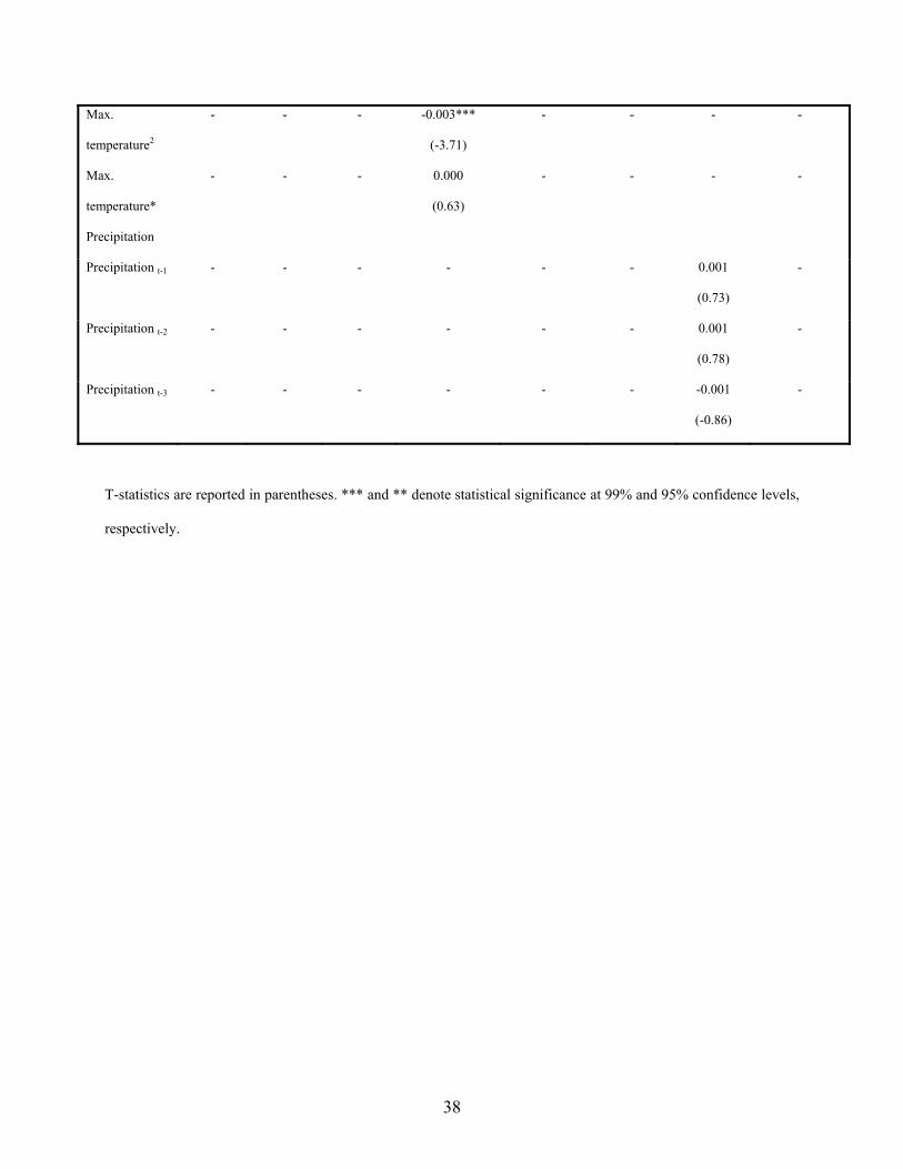
Specification (7) adds lags of precipitation for the three preceding days. This was done to deal
with possible delays in reporting property crime – property crimes may occur in periods of low
precipitation but only get reported in the succeeding days as people return from holiday. If this
was the case, the coefficients on the lags of precipitation would be negative and significant – less
rain on one day would cause an increase in the number of crimes reported in the following one to
three days. This relationship is not observed, with all three lags of precipitation being
insignificant. As an additional robustness check, a quadratic of precipitation was used and this
also indicated that property crime and precipitation have a weak relationship.
Specification (1) was used to estimate the relationship between precipitation and the two
subcategories of property crime: ‘Theft’ and ‘Burglary’ (available on request). The results
indicate that precipitation has no effect on ‘Theft’ and the effect on ‘Burglary’ is negligible (with
a positive, significant but very small coefficient).
6.5 Limitations to Empirical Work
There are several limitations to our empirical work. First, our model does not capture all the
factors that explain criminal activity. For example, alcohol consumption is likely to be correlated
with criminal activity. However, the purpose of our study is to investigate as precisely as possible
the causal effect of weather on crime rather than build a comprehensive model explaining
criminal activity. A more serious issue is that factors such as alcohol consumption may be
correlated with weather. However, this only means that our work investigates the total effect of
weather on crime: an indirect effect through its impact on daily activities as well as a direct effect
through aggression relief etc.

22
Second, spatial correlation in crime could be an issue, particularly in areas such as Auckland. For
example, higher crime in Auckland city could ‘spill over’ into neighboring police districts. We
have not explicitly dealt with this issue but we take some comfort in the large size of police
districts (average population of 94,600) and thus believe that spatial correlation does not have
significant implications for our results. If police districts were city blocks, then it would be far
more likely for a wave of burglaries to affect a cluster of city blocks. However, as our police
districts are far larger than this, spatial correlation is unlikely to be a major issue.
Third, Augmented Dickey Fuller Tests revealed that within each district, the property crime and
violent crime time series are characterized by unit roots. However, the effect of current weather
on crime in our regressions is robust to the addition of lags of the dependent variable. Our study
does not address the dynamic properties of crime beyond their effect on the coefficient estimates
for the weather variables.
Fourth, it is possible that the weather variables are statistically significant due to the large number
of observations rather than a causal relationship. In order to check whether the large number of
observations is a key reason for the significance of the weather variables, we regressed ‘Fraud’
on temperature and precipitation. We could find no theoretical reason for a relationship between
‘Fraud’ and temperature/precipitation and so we expected that temperature and precipitation
would be insignificant. Our findings confirmed this hypothesis, suggesting that the large number
of observations was not the (only) reason for the significance of precipitation and temperature in
our other results.

23
7. The Nor’wester and Violent Crime
The Nor’wester wind allegedly incites ‘disorderly’ behavior in the Canterbury region. For
example, suicide rates and domestic violence rates are said to increase (Brenstrum 1989). In this
section, we present a preliminary empirical test of this assertion, using the number of total violent
crimes as a proxy for ‘disorderly’ behavior. We do not an attempt to establish any effect of wind
in general, but instead to investigate the special alleged effect of the Nor’wester.
We use data from the Christchurch, North Canterbury and South Canterbury police districts
which are exposed to the Nor’wester. The Nor’wester is associated with warm weather. On days
when the North Westerly wind is greater than 7 meters per second (25 km/h; 16 miles/h), the
average maximum daily temperature is 20.5ºC (68.9ºF), compared to a sample mean of 17.0ºC
(62.6ºF). The mean number of total violent crimes across the three regions is 9.8. On days when
the North Westerly wind is greater than 7 meters per second, the average number of violent
crimes is 11.3, indicating a possibility of a causal relationship.
To investigate the effects of the Nor’wester, a dummy variable was constructed using wind
direction and speed (at 1 pm) and daily maximum temperature. The Nor’wester is colloquially
defined as a warm, strong wind from the North West. No formal definition of the Nor’wester
could be found and so, for our purposes, we define a Nor’wester to be a North Westerly wind that
exceeds a speed of 10 meters per second (36 km/h; 22 miles/h) and a temperature of 17ºC (63ºF)
- definition (1). The threshold for wind is based on the Beaufort wind scale which defines a ‘fresh
wind’ to be 30–39 km/h (19-24 miles/h) and the temperature threshold was chosen at the average

24
temperature for the sample. Alternative definitions of the Nor’wester were employed as
robustness checks (Table 7). OLS was used to estimate the following specification:
2, 0 1 , 2 , 3 , 4 , 3 , ,
,
,
nor'wester tempmax tempmax precip
violent offences in district on day nor'wester a dummy variable for a Nor'wester in district on da
vd t d t d t d t d t d t d t
vd t
d t
O controlswhere
O d td
β β β β β β ε= + + + + + +
==
,
,
,
y precip millimetres of precipitation in district on day
tempmax maximum temperature in district on day a set of controls
d t
d t
d t
td t
d tcontrols
===
The controls used are the same as those in specification (1) from the preceding sections. It is
worth noting that β1 in the above specification does not capture the full effect of a Nor’wester but
only any extra effect Nor’wester might have after controlling for daily temperature and
precipitation.
The coefficient on the Nor’wester is positive but insignificant across all four definitions. The
Nor’wester variable calculated using our preferred definition, definition (1), is only significant at
the 73% confidence level and so we cannot infer a strong extra effect of the Nor’wester on
violent crime. Notably, the coefficients on the temperature and precipitation variables remain
significant and of similar magnitudes to our previous findings.
Although the Nor’wester coefficient is statistically insignificant, its size is large. According to
definition (1), a Nor’wester day causes an extra 1.08 violent crimes (the sample mean is 9.80).
This is in addition to any effect of temperature or precipitation in general as both are controlled
for. While the statistical insignificance of the Nor’wester coefficient limits our ability to draw

25
strong conclusions, it appears that the Nor’wester might have an effect on the number of violent
crimes and a future study using a longer time period might address the issue.
The insignificance of the Nor’wester variable may be due to the small number of days that fit the
definition of a Nor’wester (only 42 out of 8,826 in definition (1)). In addition, wind at 1 pm was
used to represent the wind conditions for the entire day. If the wind direction and/or speed change
during the day, 1 pm wind will not be representative of the day’s wind conditions. Finally, the
number of total violent crimes may not be a good proxy for the ‘disorderly’ behavior associated
with the Nor’wester.
8. Conclusions
Our empirical work suggests that weather is an important determinant of the number of criminal
offences recorded. In particular, temperature and precipitation both have a significant effect on
the number of violent crimes recorded and temperature has a significant effect on the number of
property crimes recorded. We were unable to establish that the Nor’wester has any special effect
on the number of violent crimes committed, although there is evidence to suggest a study with
more data and a more robust measure of wind conditions may find a positive and substantial
relationship.
Our results suggest that police should respond to weather shocks characterized by increases in
temperature and/or decreases in precipitation by increasing the resources allocated to policing on
those days. For example, additional patrols of residential areas could be undertaken in ‘fine’
weather in response to an anticipated increase in property crime. Importantly, however, our

26
models are only estimating the effects of unexpected (i.e., not given by geography and season)
weather changes. Thus, when allocating its resources, police should use information on both
district and seasonal characteristics (e.g., January in Auckland) and current weather conditions
(from short-term weather forecast) into account.
Our study is limited in several ways. First, the police districts are often too large for us to
generate representative weather variables. However, if anything, this is likely to bias our results
downwards. Second, as discussed above, there are potential issues with variation in policing as
weather changes. To the extent that police effort already responds to weather changes as
recommended here, our results are again a conservative estimate of the true effect of weather on
crime. Third, we do not have data available for a number of variables that affect crime. However,
our research is a partial analysis of the effect of weather on crime; we do not aim to explain all
variation in crime levels.
Despite the above limitations, our study makes several significant contributions. Most
importantly, we use a large and detailed dataset and demonstrate that the relationship between
weather and crime remains robust to different model specifications. Our empirical results are
largely consistent with our theoretical framework and previous studies and provide solid
recommendations for the allocation of police resources.

27
References
Becker, G., 1968. ‘Crime and Punishment: An Economic Approach’ Journal of Political
Economy, 76(3):169-217.
Bell, P., 1992. ‘In Defense of the Negative Affect Escape Model of Heat and Aggression’
Psychological Bulletin, 111: 342-346.
Brenstrum, E., 1989. ‘Canterbury’s Damaging Nor'wester’.
(http://vaac.metservice.com/default/index.php?alias=norwester192956; Accessed
12/10/2009)
Cohn, E., 1990. ‘Weather and Crime’ British Journal of Criminology, 30: 51-64.
Cohn, E. and Rotton, J., 2000a. ‘Violence Is a Curvilinear Function of Temperature in Dallas: A
Replication’ Journal of Personality and Social Psychology, 78: 1074-1081.
Cohn, E. and Rotton, J., 2000b. ‘Weather, Disorderly Conduct, and Assaults: From Social
Contract to Social Avoidance’ Environment and Behavior, 32: 651-673.
Cohn, E. and Rotton, J., 2000c. ‘Weather, Seasonal Trends and Property Crimes in Minneapolis,
1987-88. A Moderator-Variable Time-Series Analysis of Routine Activities’ Journal of
Environmental Psychology, 20: 257-272.
Felson, M., 1987. ‘Routine Activities and Crime Prevention in the Developing Metropolis’
Criminology, 25: 911-931.
Field, S., 1992. ‘The Effect of Temperature on Crime’ British Journal of Criminology, 32: 340-
351.
28
Jacob, B., Lefgren, L., and Moretti, E., 2006. ‘The Dynamics of Criminal Behavior: Evidence
from Weather Shocks’ Journal of Human Resources, 42: 489-527.
Papps, K. and Winkelmann, R., 2000. ‘Unemployment and Crime: New Evidence for an Old
Question’ New Zealand Economic Papers, 43:1 53-71.
Schmallenger, F., 1997. Criminal Justice Today, Englewood Cliffs, New Jersey.
Sjoquist, D.L., 1973. ‘Property Crime and Economic Behavior: Some Empirical Results’
American Economic Review, 63: 439-446.

29
Figure 1. The Estimated Effect of Temperature on Violent Crime

30
Figure 2. The Estimated Effect of Temperature on Property Crime

31
Table 1. Categories of Crime Data Provided by the New Zealand Police
Aggregated Data Available Prominent Subcategories
Violence Forms of assault (~70%), intimidation and threats (~15%), homicide (~0.3%)
Sexual Indecent assault (~35%), sexual violation (~20%)
Drugs and Anti-social Cannabis use (~45%), disorder (~35%)
Property Damage Willful damage (~90%)
Property Abuse Trespass (~65%)
Administrative Offences against justice (~80%)
Burglary Burglary - day (~40%) Burglary - night (~40%)
Car Conversion Etc Unlawful taking of a car (~50%), Unlawful interference with a car (~40%)
Fraud Document fraud (~50%), bank card fraud (~20%)
Receiving Receiving stolen goods (~95%)
Theft Shoplifting (~50%), theft under $500 (~25%)
The approximate weightings of the subcategories were obtained by analyzing annual data from Statistics New
Zealand. Unfortunately, the daily data provided to us could not be disaggregated into these subcategories. However,
even if data for the narrow subcategories could be obtained, many district/day values would be zero.
32
Table 2. Crime and Weather Descriptive Statistics
All Max. temperature<14 ºC Max. temperature>27 ºC Precipitation>10mm Min Max
Total Violent (per day, per
district)
7.21 6.80 6.35 6.46 0.00 108.00
Violence 3.09 2.61 2.68 2.86 0.00 54.00
Property Abuse 1.24 1.14 1.03 1.14 0.00 95.00
Property Damage 2.88 3.05 2.64 2.46 0.00 103.00
Total Property (per day,
per district)
11.79 10.66 9.26 11.50 0.00 202.00
Theft 7.94 7.37 6.15 7.64 0.00 200.00
Burglary 3.85 3.29 3.11 3.85 0.00 115.00
Daily Maximum Temp (ºC) 11.75 2.52 36.06
Daily Precipitation (mm) 3.51 0.00 240.60
Total Observations 141,384 25,680 3,820 13,636

33
Table 3. The Effects of Temperature on Violent Crime
Spec (1) Spec (2)
(Spec 1 +
popul.
weights)
Spec (3)
(Spec 2 +
crime
lags)
Spec (4)
(Spec 3 +
precip.)
Spec (5)
(Spec 1
with
crimes/
100,000)
Spec (6)
(Spec 1
with
Tobit)
Spec (7)
(Spec 1 +
aver. temp
in prev. 7
days)
Spec (8)
(Spec 1 +
district t-
trend)
R2 0.432 0.407 0.412 0.413 0.396 0.095 0.432 0.439
0.126*** 0.169*** 0.149*** 0.147*** 0.145*** 0.130*** 0.128*** 0.132*** Max. temperature
(7.30) (7.43) (6.60) (6.46) (6.05) (7.32) (7.28) (7.61)
-0.002*** -0.003*** -0.003*** -0.003*** -0.003*** -0.003*** -0.002*** -0.003*** Max. temperature2
(-5.20) (-5.56) (-5.09) (-5.19) (-4.07) (-5.24) (-5.11) (-5.56)
-0.007 Average temperature in
preceding seven days
- - - - - -
(-0.94)
-
0.083*** 0.082*** Violent crimes t-1 - -
(21.38) (20.92)
- - - -
0.013*** 0.012*** Violent crimes t-2 - -
(3.57) (3.48)
- - - -
0.000 0.000 Violent crimes t-3 - -
(0.17) (0.11)
- - - -
0.021*** Precipitation - - -
(2.78)
- - - -
0.000 Max. temperature
*Precipitation
- - -
(0.06) -
- - -
T-statistics are reported in parentheses. *** denotes statistical significance at 99% confidence level.

34
Table 4. The Effects of Precipitation on Violent Crime
Spec (2) Spec (3) Spec (4) Spec (5) Spec (6) Spec (7) Spec (8) Spec (1)
(Spec 1 +
popul. weights)
(Spec 2 +
crime lags)
(Spec 3 +
temp.)
(Spec 1 with
crimes/ 100,000)
(Spec 1 with
Tobit)
(Spec 1 +
precip2)
( Spec 1 +
district t-
trend)
R2 0.432 0.409 0.414 0.413 0.396 0.095 0.432 0.440
-0.019*** -0.024*** -0.021*** -0.021*** -0.022*** -0.020*** -0.026*** -0.019*** Precipitation
(-14.38) (-14.20) (-12.87) (-2.78) (-11.76) (-14.30) (-9.74) (-14.44)
0.083*** 0.082*** Violent crimes t-1 - -
(21.34) (20.92)
- - - -
0.013*** 0.012*** Violent crimes t-2 - -
(3.69) (3.48)
- - - -
0.000 0.000 Violent crimes t-3 - -
(0.14) (0.11)
- - - -
0.147*** Max. temperature - - -
(6.46)
- - - -
-0.003*** Max.
temperature2
- - -
(-5.19)
- - - -
0.000*** Max.
temperature*
Precipitation
- - -
(0.06)
- - - -
0.000*** Precipitation2 - - - - -
(2.79)
-
T-statistics are reported in parentheses. *** denotes statistical significance at 99% confidence level.

35
Table 5. The Effects of Temperature on Property Crime
Spec (1) Spec (2)
(Spec 1 +
popul.
weights)
Spec (3)
(Spec 2 +
crime lags)
Spec (4)
(Spec 3 +
precip.)
Spec (5)
(Spec 1 with
crimes/
100,000)
Spec (6)
(Spec 1
with
Tobit)
Spec (7)
(Spec 3 +
aver.
temp in
prev. 7
days)
Spec (8)
(Spec 1 +
district t-
trend)
R2 0.685 0.636 0.657 0.657 0.6882 0.165 0.702 0.694
Max. temperature 0.106***
(5.34)
0.152***
(5.49)
0.119***
(4.41)
0.117***
(4.28)
0.068**
(2.47)
0.107***
(5.34)
0.089***
(4.53)
0.104***
(5.32)
Max. temperature2 -0.003***
(-4.76)
-0.004***
(-4.78)
-0.003***
(-3.83)
-0.003***
(-3.71)
-0.002**
(-2.40)
-0.003***
(-4.76)
-0.002***
(-3.91)
-0.003***
(-4.81)
Property crimes t-1 - - 0.11***
(23.49)
0.11***
(23.47)
- - 0.112***
(28.48)
-
Property crimes t-2 - - 0.055***
(13.23)
0.054***
(13.17)
- - 0.057***
(16.09)
-
Property crimes t-3 - - 0.053***
(13.12)
0.053***
(13.06)
- - 0.055***
(16.35)
-
Property crimes t-4 - - 0.047***
(11.89)
0.047***
(11.93)
- - 0.046***
(13.63)
-
Property crimes t-5 - - 0.037***
(8.95)
0.037***
(8.91)
- - 0.04***
(11.75)
-
Property crimes t-6 - - 0.051***
(13.08)
0.051***
(13.13)
- - 0.05***
(15.25)
-
Property crimes t-7 - - 0.078***
(19.08)
0.078***
(19.08)
- - 0.075***
(22.19)
-
Property crimes t-8 - - 0.034*** 0.034*** - - 0.034*** -

36
(8.87) (8.86) (10.72)
Property crimes t-9 - - 0.025***
(6.56)
0.025***
(6.52)
- - 0.025***
(7.86)
-
Precipitation - - - 0.001
(0.10)
- - - -
Max. temperature*
Precipitation
- - - 0.000
(0.63)
- - - -
Average temperature in
preceding seven days
- - - - - - -0.024***
(-3.09)
-
T-statistics are reported in parentheses. *** and ** denote statistical significance at 99% and 95% confidence levels,
respectively.

37
Table 6. The Effects of Precipitation on Property Crime
Spec (1) Spec (2)
(Spec 1 +
popul.
weights)
Spec (3)
(Spec 2 +
crime
lags)
Spec (4)
(Spec 3 +
temp.)
Spec (5)
(Spec 1 with
crimes/
100,000)
Spec (6)
(Spec 1 with
Tobit)
Spec (7)
(Spec 1 +
precip.
lag)
Spec (8)
(Spec 1 +
district t-
trend)
R2
0.685
0.638
0.659
0.657
0.688
0.165
0.685
0.694
Precipitation 0.004***
(2.73)
0.007***
(3.24)
0.006***
(3.06)
0.001
(0.10)
0.003
(1.62)
0.004**
(2.54)
0.004**
(2.38)
0.004***
(2.65)
Property
crimes t-1
- - 0.111***
(23.75)
0.110***
(23.47)
- - -
Property
crimes t-2
- - 0.055***
(13.24)
0.054***
(13.17)
- - - -
Property
crimes t-3
- - 0.053***
(13.11)
0.053***
(13.06)
- - - -
Property
crimes t-4
- - 0.047***
(11.99)
0.047***
(11.93)
- - - -
Property
crimes t-5
- - 0.036***
(8.86)
0.037***
(8.91)
- - - -
Property
crimes t-6
- - 0.052***
(13.27)
0.051***
(13.13)
- - - -
Property
crimes t-7
- - 0.078***
(19.22)
0.078***
(19.08)
- - - -
Property
crimes t-8
- - 0.034***
(8.85)
0.034***
(8.86)
- - - -
Property
crimes t-9
- - 0.025***
(6.53)
0.025***
(6.52)
- - - -
Max.
temperature
- - - 0.117***
(4.28)
- - - -
38
Max.
temperature2
- - - -0.003***
(-3.71)
- - - -
Max.
temperature*
Precipitation
- - - 0.000
(0.63)
- - - -
Precipitation t-1 - - - - - - 0.001
(0.73)
-
Precipitation t-2 - - - - - - 0.001
(0.78)
-
Precipitation t-3 - - - - - - -0.001
(-0.86)
-
T-statistics are reported in parentheses. *** and ** denote statistical significance at 99% and 95% confidence levels,
respectively.

39
Table 7. The Effects of the Nor’wester Wind on Violent Crime
Definition (1) Definition (2) Definition (3) Definition (4)
Definition
North West wind
Max. temperature>17ºC
Wind speed>36km/h
North West wind
Max. temperature>15ºC
Wind speed>25km/h
North West wind
-
Wind speed>36km/h
North West wind
Max. temperature>25ºC
Wind speed>25km/h
Number of Nor’wester days 42 169 45 22
Nor’wester
1.078
(1.12)
0.578
(1.60)
0.890
(0.98)
1.136
(1.23)
Max. temperature
0.157***
(3.36)
0.155***
(3.32)
0.156***
(3.36)
0.161***
(3.46)
Max. temperature2
-0.004***
(-3.08)
-0.004***
(-3.06)
-0.004***
(-3.07)
-0.004***
(-3.19)
Precipitation
-0.059***
(-7.39)
-0.059***
(-7.38)
-0.059***
(-7.39)
-0.059***
(-7.40)
T-statistics are reported in parentheses. *** denotes statistical significance at 99% confidence level.


![Forecasting Crime with Deep Learning - arXiv · crime data. We make use of weather data, census data, and public transportation data on top of the crime reports. Cohn [4] establishes](https://img.pdfslide.us/doc/110x75/5f66a77ca7fa7c529521e9f8/forecasting-crime-with-deep-learning-arxiv-crime-data-we-make-use-of-weather.jpg)