Embed Size (px)
Citation preview
IZA DP No. 1032
The Effects of Wealth and Incomeon Subjective Well-Being and Ill-Being
Bruce HeadeyMark Wooden
DI
SC
US
SI
ON
PA
PE
R S
ER
IE
S
Forschungsinstitutzur Zukunft der ArbeitInstitute for the Studyof Labor
February 2004
The Effects of Wealth and Income on Subjective Well-Being and Ill-Being
Bruce Headey Melbourne Institute of Applied Economic and Social Research
Mark Wooden Melbourne Institute of Applied Economic and Social Research
and IZA Bonn
Discussion Paper No. 1032 February 2004
IZA
P.O. Box 7240 53072 Bonn
Germany
Phone: +49-228-3894-0 Fax: +49-228-3894-180
Email: [email protected]
Any opinions expressed here are those of the author(s) and not those of the institute. Research disseminated by IZA may include views on policy, but the institute itself takes no institutional policy positions. The Institute for the Study of Labor (IZA) in Bonn is a local and virtual international research center and a place of communication between science, politics and business. IZA is an independent nonprofit company supported by Deutsche Post World Net. The center is associated with the University of Bonn and offers a stimulating research environment through its research networks, research support, and visitors and doctoral programs. IZA engages in (i) original and internationally competitive research in all fields of labor economics, (ii) development of policy concepts, and (iii) dissemination of research results and concepts to the interested public. IZA Discussion Papers often represent preliminary work and are circulated to encourage discussion. Citation of such a paper should account for its provisional character. A revised version may be available on the IZA website (www.iza.org) or directly from the author.
IZA Discussion Paper No. 1032 February 2004
ABSTRACT
The Effects of Wealth and Income on Subjective Well-Being and Ill-Being∗
The accepted view among psychologists and economists alike is that household income has statistically significant but only small effects on measures of subjective well-being. Income, however, is clearly an imperfect measure of the economic circumstances of households. Using data drawn from the 2001 and 2002 waves of the Household, Income and Labour Dynamics in Australia (HILDA) Survey, this paper demonstrates that wealth, which can be viewed as providing a degree of economic security, is at least as important to well-being and ill-being as income. JEL Classification: D19 Keywords: income, wealth, subjective well-being, life satisfaction Corresponding author: Mark Wooden Melbourne Institute of Applied Economic and Social Research Faculty of Economics and Commerce University of Melbourne Melbourne, VIC 3010 Australia Email: [email protected]
∗ This paper reports on research being conducted as part of the research program, “The Dynamics of Economic and Social Change: An Analysis of the Household, Income and Labour Dynamics in Australia Survey”. It is supported by an Australian Research Council Discovery Grant (DP0342970). The paper uses the data in the confidentialized unit record file from the Department of Family and Community Services’ (FaCS) Household, Income and Labour Dynamics in Australia Survey, which is managed by the Melbourne Institute of Applied Economic and Social Research. The findings and views reported in the paper, however, are those of the authors and should not be attributed to either FaCS or the Melbourne Institute.
1
I Introduction
The accepted view in psychology is that objective economic circumstances
have only a slight though statistically significant effect on happiness and other
measures of well-being (Andrews and Withey 1976; Argyle 1987; Campbell,
Converse and Rodgers 1976; Diener and Biswas-Diener 2002; Diener et al. 1999;
Headey and Wearing 1992; Kahnemann, Diener and Schwarz 1999). This view has
sometimes been repeated by economists, usually with reference to Easterlin’s seminal
1974 paper, ‘Does economic growth improve the human lot?’ However, the claim that
money has little effect on happiness is almost entirely based on weak relationships
between survey measures of happiness and measures of income. The single exception
appears to be a paper by Mullis (1992), which was based on a sample of American
men aged between 55 and 69 years of age, and showed that, for this group, income
and wealth combined additively to affect scores on a composite index of satisfaction
with standard of living, housing, neighbourhood, health, leisure and ‘life in general’.
Plainly income is not the only or necessarily the best indicator of material
standard of living. Using data from the new Household, Income and Labour
Dynamics in Australia (HILDA) Survey, this paper estimates the combined effects of
disposable income and wealth (net worth) on measures of subjective well-being
(SWB) and ill-being. The analysis indicates that objective economic circumstances
have a greater impact on subjective outcomes than previously believed.
We stress that this paper assesses the impact of economic circumstances on ill-
being (or psychological distress) as well as well-being (or happiness). So far as we
know, it is the first paper which imports into economics a key result from the
psychological literature – namely that well-being and ill-being are distinct dimensions

2
and not opposite ends of the same dimension (Bradburn 1969; Diener 1984; Diener et
al. 1999; Headey Kelley and Wearing 1993; Headey and Wearing 1992). The issue
here is whether objective economic circumstances do more to promote well-being or
relieve ill-being, or have about the same impact on both. Our results provide most
support for the latter hypothesis.
II Economic and Psychological Theory
Until very recently, the two major social science literatures on happiness and
well-being – the economic literature on utility and the psychological literature on
SWB – steadfastly ignored each other. Welfare economists learn not to measure
utility directly, but instead to infer it from behaviour. Following Samuelson (1938),
the standard approach is to treat behaviours as ‘revealed preferences’. Utility is
viewed as involving trade-offs between work and leisure. Work is regarded as pain
but provides the wherewithal for consumption, while leisure is regarded as pleasure.
Individuals are viewed as making different trade-offs, depending on their preferences
for consumption and leisure, but essentially a happy person is seen as someone with a
full shopping basket and lots of free time; a rather hedonistic view.
In psychology, empirical research on well-being and happiness began in the
late 1960s and 1970s at the Universities of Chicago (Bradburn 1969 and Michigan
(Andrews and Withey 1976; Campbell, Converse and Rodgers 1976). The early
studies made two discoveries that are still debated but are accepted by the large
majority of researchers. These discoveries, if correct, are of great importance to
economists.
3
First, well-being (or happiness) and ill-being (or psychological distress) are
empirically distinct dimensions with different causes; they are not opposite ends of
the same dimension. Well-being comprises life satisfaction and positive feelings (e.g.,
joy, vitality), or what psychologists call positive affects. Ill-being comprises anxiety,
depression and other negative affects. There is much evidence that people can
experience both high levels of well-being and also quite high levels of anxiety at the
same time (see Headey, Kelley and Wearing 1993).
Second, economic variables, notably income, appear to have little effect on
either well-being or ill-being. This is part of a more general finding that objective
circumstances of all kinds (such as gender, age and employment status) have only
modest effects on subjective outcomes. Well-being turns out to be much more
affected by personality traits, personal relationships and social participation, and ill-
being by personality problems, marital problems, job problems (including
unemployment) and self-assessed health.
In recent years, economists have begun to take an interest in the psychological
literature (see Frey and Stutzer 2002 for a review). An important motivation for the
recent interest among economists in psychological theories and results relating to
well-being is a concern that the ‘revealed preferences’ approach may be open to
challenge. This approach depends on the assumption that people’s preferences for
goods and leisure are exogenously determined and hence that increases in supply will
increase utility. However, if people change their preferences in response to what
others have and want, as proposed by Duesenberry (1949), then one cannot
reasonably infer that more goods and leisure, preferred at time t, will necessarily
increase utility if acquired at time t+1. Easterlin (1974) provided support for
Duesenberry’s theory by showing that, in so far as income affects happiness at all, it
4
is relative income – one’s income relative to others in one’s own country – and not
absolute gains in income that make a difference. A recent issue of the Journal of
Economic Behavior and Organization (July, 2001; see especially Hollaender, pp. 227-
49) was devoted to the debate about whether preferences are exogenous or
endogenous, and the major implications for welfare economics of accepting the latter
standpoint (see also Frank 1985).
Some economists might concede that, while it might be desirable to measure
utility directly, it cannot be done in a reasonably valid way. Economists have been
trained to the view that it is impossible to make interpersonal comparisons of utility.
Can anyone really believe, they ask, that a person who scores 80 on a survey measure
of satisfaction is more satisfied than someone who scores 70 or 75? Psychologists
who have developed measures of well-being might reply that, taken literally, no-one
does believe that. But, they might also reply, do economists literally believe that
someone who reports an income of $80,000 in a survey or a tax return really has a
higher income than someone who reports $70,000 or $75,000? What the
psychologists claim is that, in general, the people who score higher on satisfaction
scales are more satisfied than people who score lower, and ‘in general’ is all that is
needed for statistical analysis or, one might add, for business and government
decision-making.
A limitation of the recent work in economics is a lack of recognition that well-
being is probably better regarded as multi-dimensional, not unidimensional. To date
those economists who have reported results involving direct measurement of well-
being have usually conceptualized it as ‘satisfaction’; either life satisfaction or
satisfaction with one’s material standard of living or financial situation. So far as we

5
know, no previous research has investigated the impact of economic circumstances on
ill-being, as well as well-being.
III Data and Methods
(i) The HILDA Survey
The data for this analysis come from the second wave of the HILDA Survey,
conducted in 2002. Described in more detail in Watson and Wooden (2002), the
HILDA Survey is a household panel survey. It began with a large national probability
sample of households, and involved personal interviews with all household members
aged 15 years and over. In wave 1, conducted during the second half of 2001,
interviews were obtained at 7682 households, which represent 66 per cent of all
households identified as in-scope. This, in turn generated, a sample of 15,127 persons
eligible for interview, 13,969 of whom were successfully interviewed.
A year later all responding households from wave 1 were re-contacted.
Interviews were again sought with all household members aged 15 years or over,
including persons who did not respond in wave 1, as well as any new household
members. In total, interviews were completed with 13,041 persons from 7245
households. Of this group almost 12,000 were respondents from wave 1, which
represents almost 87 per cent of the wave 1 individual sample.
The coverage of the survey is extremely broad, but with a focus on household
structure and formation, income and economic well-being, and employment and
labour force participation. Each year a special module of non-core questions is added.
In wave 1 it was appropriate to devote the module to personal and family history. In
wave 2 the topic was wealth. Each year’s survey also includes a leave-behind self-

6
completion questionnaire, which mainly contains attitude questions. Among the topics
covered are experiences of financial stress and deprivation, social networks, attitudes
to saving and borrowing, and physical and psychological health.
For this paper we restrict the sample to persons of prime working age (25-59
years) at 30 June 2002, reducing the final sample to 7934 observations. This exclusion
seems justified on the grounds that the economic concerns of younger people and
retirees tend to be quite different from the prime age group. Younger people typically
do not expect to earn much – many are still in education – and retirees, being mostly
not in paid work, care primarily about their superannuation assets and pension
income.
Cross-sectional weights have been used in reporting means and standard
deviations, and for making ‘predictions’ about the impact of economic circumstances
on SWB. As is usual, weights were not used in regression analyses.
(ii) Well-being Measures
Two indicators of subjective well-being were used and two of ill-being. The
well-being indicators were single item measures of ‘overall life satisfaction’ and
‘satisfaction with your financial situation’. The ill-being measures were a 5-item scale
based on the mental health sub-scale included in the SF-36 Health Survey and a
measure of ‘financial stress’ constructed from eight questions about difficulty in
paying bills and dealing with financial emergencies (see below). It should be noted
that, both for well-being and ill-being, one measure relates to the concept defined very
broadly and one relates specifically to the economic/financial domain of life.
The concept of life satisfaction is perhaps closest to what welfare economists
say they mean by utility, and is the concept employed in nearly all the recent studies

7
by economists who have chosen to measure utility directly. On the other hand,
‘satisfaction / dissatisfaction with your financial situation’, or satisfaction /
dissatisfaction with material standards of living, seem to be the outcomes most likely
to result from the variables that are actually included in most welfare economics
equations and from the variables measuring family economic circumstances, which
are our focus here.
Life satisfaction and financial satisfaction were both measured by single
questions scored on a 0-10 scale. Only the extreme values were labeled, with a score
of 0 described as ‘totally dissatisfied’ and a score of 10 as ‘totally satisfied’. For ease
of interpretation these scales – and the ill-being measures also – were rescored to run
from 0 to 100. This means that the coefficients in regression results can be understood
as showing the quasi-percentage increases or decreases in well-being or ill-being that
would result from one unit of change in the explanatory variable in question (net of
the effects of other variables on the right hand side).
Clearly, single item scales are not the best measures of well-being available,
but they are very widely used in international surveys and have been found to have
acceptable levels of reliability and validity (Diener et al. 1999, pp. 277-278). It
appears that, in relation to life satisfaction in particular, human beings can make quick
global judgments in survey interviews; judgments which pretty accurately summarize
their feelings. The global judgments that individuals make about themselves are
corroborated by external validity tests done with partners and friends (Diener et al.
1999). Judgments of life satisfaction prove to be reasonably stable; they have a test-
retest reliability of around 0.6, which is about the same as standard tests of blood
pressure.
8
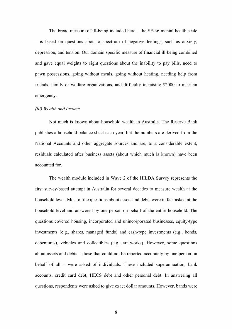
The broad measure of ill-being included here – the SF-36 mental health scale
– is based on questions about a spectrum of negative feelings, such as anxiety,
depression, and tension. Our domain specific measure of financial ill-being combined
and gave equal weights to eight questions about the inability to pay bills, need to
pawn possessions, going without meals, going without heating, needing help from
friends, family or welfare organizations, and difficulty in raising $2000 to meet an
emergency.
(iii) Wealth and Income
Not much is known about household wealth in Australia. The Reserve Bank
publishes a household balance sheet each year, but the numbers are derived from the
National Accounts and other aggregate sources and are, to a considerable extent,
residuals calculated after business assets (about which much is known) have been
accounted for.
The wealth module included in Wave 2 of the HILDA Survey represents the
first survey-based attempt in Australia for several decades to measure wealth at the
household level. Most of the questions about assets and debts were in fact asked at the
household level and answered by one person on behalf of the entire household. The
questions covered housing, incorporated and unincorporated businesses, equity-type
investments (e.g., shares, managed funds) and cash-type investments (e.g., bonds,
debentures), vehicles and collectibles (e.g., art works). However, some questions
about assets and debts – those that could not be reported accurately by one person on
behalf of all – were asked of individuals. These included superannuation, bank
accounts, credit card debt, HECS debt and other personal debt. In answering all
questions, respondents were asked to give exact dollar amounts. However, bands were
9
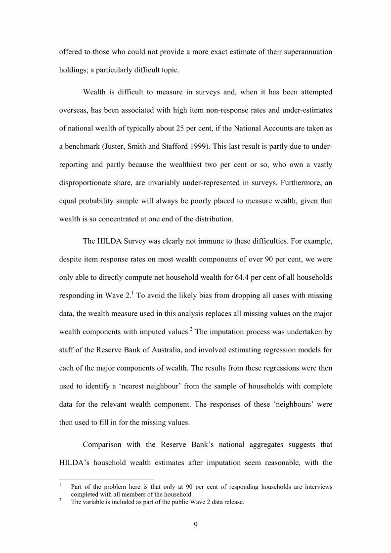
offered to those who could not provide a more exact estimate of their superannuation
holdings; a particularly difficult topic.
Wealth is difficult to measure in surveys and, when it has been attempted
overseas, has been associated with high item non-response rates and under-estimates
of national wealth of typically about 25 per cent, if the National Accounts are taken as
a benchmark (Juster, Smith and Stafford 1999). This last result is partly due to under-
reporting and partly because the wealthiest two per cent or so, who own a vastly
disproportionate share, are invariably under-represented in surveys. Furthermore, an
equal probability sample will always be poorly placed to measure wealth, given that
wealth is so concentrated at one end of the distribution.
The HILDA Survey was clearly not immune to these difficulties. For example,
despite item response rates on most wealth components of over 90 per cent, we were
only able to directly compute net household wealth for 64.4 per cent of all households
responding in Wave 2.1 To avoid the likely bias from dropping all cases with missing
data, the wealth measure used in this analysis replaces all missing values on the major
wealth components with imputed values.2 The imputation process was undertaken by
staff of the Reserve Bank of Australia, and involved estimating regression models for
each of the major components of wealth. The results from these regressions were then
used to identify a ‘nearest neighbour’ from the sample of households with complete
data for the relevant wealth component. The responses of these ‘neighbours’ were
then used to fill in for the missing values.
Comparison with the Reserve Bank’s national aggregates suggests that
HILDA’s household wealth estimates after imputation seem reasonable, with the
1 Part of the problem here is that only at 90 per cent of responding households are interviews
completed with all members of the household. 2 The variable is included as part of the public Wave 2 data release.
10
HILDA Survey appears to have under-estimated net worth by only around 10 per cent
(see Headey, Marks and Wooden forthcoming). This is likely to be almost entirely
due to inadequate representation of the very wealthy. Our wealthiest household, for
example, had a reported net worth of $22 million, which is well below the levels
recorded for individuals listed in the BRW list of Australia’s 200 wealthiest people.
Note that the variable we use to measure wealth is net worth at the household
level. In other words, even where questions were asked at the individual level, we
have summed the results for all household members and attributed the same net worth
to each person.
Turning now to income, individual respondents are asked each wave to
provide extensive details about their income from all sources during the preceding
financial year. That includes labour income (wages and salaries), asset income
(business income, rental income, share dividends, etc.), private superannuation
income, private transfers (e.g., child support payments) and public transfers (pensions,
benefits). Like all other surveys, HILDA does not ask about taxes, since most people
could not answer accurately. So in order to estimate disposable incomes, taxes have to
be imputed. Again, there is a problem with missing data, with the necessary data to
construct household income missing in almost 28 per cent of cases in wave 2. So we
again used the household income variable provided in the data file that includes
imputed estimates for missing cases.
The main measure of income used in this paper is household disposable
income, which, with a couple of adjustments (discussed below), is usually regarded as
the best income-based measure of material standard of living. As with wealth, our
measure is based on summing the incomes of all household members and implicitly
assuming that resources are shared.
11
Obviously a small household with the same income as a large household
would have a higher standard of living, so it is necessary to make some adjustment for
household size. The obvious way to do this is to calculate household per capita
income, but this makes no allowance for economies of scale in larger households or
for the fact that children are cheaper to keep than adults. The usual way to make the
adjustment is to use an equivalence scale; a scale intended to assist measurement of
standard of living by adjusting household income to needs. In this paper the
equivalence scale we use is the so-called International Experts’ Scale, which
represents a compromise among the wide range of scales explicitly or implicitly used
by Western governments in running their social assistance programs (Buhmann et al.
1988). Use of the scale requires dividing household disposable income by the square
root of household size. So a four-person household with a disposable income of
$40,000 is deemed to have an equivalent income of $20,000.3 Note that we did not
equivalize wealth (net worth) because, for reasons unclear, equivalized wealth
correlated with dependent variables much less strongly than the unequivalized
variable.
A further measurement issue was whether to use logarithmic transformations
of wealth and income in regression equations. Economists normally prefer to take
logs of income-like measures because the distributions are usually lognormal rather
than normal, due to small numbers of very rich people (in the right tail of the
distribution). Inspection of the data for wealth indicated the necessity of a log
transformation. However, equivalized disposable income has a more or less normal
distribution, so a log transformation is not a statistical necessity. Empirically in
Australia, and in other countries, equivalized income correlates a little more highly
3 Results are very close to those obtained for the current OECD scale of 1.0 for the first adult in a
household, 0.5 for other adults and 0.3 for children.
12
with measures of well-being and ill-being than the log of equivalized income. So on
empirical grounds we did not take logs.
IV Results
(i) Well-being
By international standards, Australians score high on well-being, with a mean
score for this age group of 77.0 on the 0-100 scale. We also find that women are
slightly more likely to report higher levels of life satisfaction than men (mean = 77.5
compared with 76.5 for men), a result different from most other Western countries,
but one that is found in all Australian studies that we have seen.
The Pearson correlations between measures of household economic
circumstances and well-being give a first clue to the fact that we are going to find
stronger relationships than in previous research. The simple correlations between
equivalized disposable income and life satisfaction, and between income and financial
satisfaction, are 0.11 and 0.27 respectively, very similar to what has been reported in
previous research. However, the correlations with wealth are actually higher than for
income; 0.15 for life satisfaction and 0.33 for financial satisfaction.
Of course these preliminary results could prove deceptive. We now assess the
combined effects of wealth and income, and also control for a small number of other
‘objective’ characteristics of respondents; sex, age, marital status, educational
attainment, employment status and disability status.4 Ordinary least squares (OLS)
4 The construction of most of these control variables is straightforward and should require little by
way of explanation. The exception here is disability status. Respondents were classified as disabled if they had any long-term health condition, impairment or disability that restricted their everyday activities and had lasted, or was likely to last, for 6 months more. Following Shields and Wooden (2003), we then further decomposed this group into three sub-groups according to the severity of
13
regression was used, although it is recognized that, strictly speaking, three of the
dependent variables are only ordinal. However, ordered probit equations gave results
that were qualitatively the same, so like most previous researchers in the field of
SWB, we preferred to give the more readily interpretable OLS results.5 Note that,
given the evidence of heteroscedasticity, all equations have been estimated with
robust standard errors.
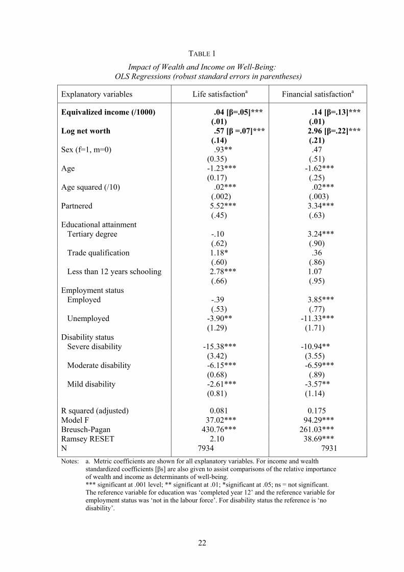
Using the evidence in Table 1 to reconsider the effects of objective economic
circumstances on well-being, one is faced with the standard worry about whether to
see the bottle as half empty or half full. Clearly the inclusion of wealth helps to
account for more variance than just income by itself. One slightly crude way to
compare the relative importance of wealth and income to well-being is to compare the
size of standardized coefficients (Betas). In Table 1 the Betas for wealth are higher
than for income in both equations. In the case of life satisfaction, it appears that the
wealth variable is just slightly more ‘important’ than the income variable (Beta=0.07
compared with 0.05), whereas for financial satisfaction the difference is much greater
(0.22 compared with 0.13). On the other hand, the combined effect of all ‘objective’
variables, including those measuring economic circumstances, is such as to account
for just 8.1 per cent of the variance in life satisfaction and a more solid 17.5 per cent
of the variance in the domain-specific measure of financial satisfaction.
It should be recorded that results were very similar when the equations were
estimated separately for men and women. Also, only minor differences were found
the disability based on how much the disability limited the type or amount of work thy could undertake. Those who could do no work at all were classified as severely disabled. Those whose disability had no impact on their ability to work were classified as mildly disabled. All other disabled persons were classified as having a moderate disability.
5 The measure of financial ill-being is actually a count of the number of different types of financially stressful events experienced in the last year. A more appropriate estimator for this type of data is provided by the Poisson regression model. Again, however, estimates from this model were qualitatively very similar to the least squares regression estimates.

14
when additional control variables were introduced. These included measures of
occupational status and home ownership.
In order to get a better handle on the key empirical issue, we now estimate
differences in well-being that would result from being at sharply different points in
the distributions of both wealth and income. Imagine two people, one at the 25th
percentile on both measures and one at the 75th percentile. These people are quite far
apart, but panel studies show that moving this far up or down the ladder is not
uncommon over, say, a decade (Goodin et al. 1999). Straightforward arithmetic, based
on the evidence in Table 1, shows that a person who moved up the ‘economic ladder’
by these 50 steps would gain 2.0 percentiles on the life satisfaction scale and 8.7
percentiles on the financial satisfaction scale. Conversely someone who dropped 50
rungs on the ladder would drop by these percentiles. The gains and losses would be
about equally due to wealth and disposable income. The 2.0 percentile gain in life
satisfaction would be 1.1 percentiles due to wealth and 0.9 due to income. The 8.7
percentiles gain in financial satisfaction breaks down into 3.4 percentiles due to
income and 5.3 due to wealth.
Continuing with the issue of whether the bottle is half empty or half full,
similar calculations show that moving 50 percentiles up the economic ladder brings
less than half the gain in life satisfaction that comes from getting married or partnered
(which brings a gain of 5.5 percentiles), but is better than getting married as a means
of increasing financial satisfaction, although getting married is not bad for that either
(gain = 3.3 percentiles). Another comparison can be made with unemployment.
Getting a job increases life satisfaction by 4.3 percentiles and increases financial
satisfaction by 15.2 percentiles; both these gains are clearly larger than the effects of
moving up the economic ladder. On the other side of the ledger, moving up or down
15
the economic ladder makes a far bigger difference than is found between women and
men (women are a little happier, as noted above), between older and younger people
(older people are a little happier), or between homeowners and tenants (homeowners
are happier).
Overall, the results presented here suggest that wealth is more important for
well-being than income. Moreover, we expect our results to understate the relative
importance of wealth given it is almost certainly not as well measured, which usually
has the effect of attenuating statistical relationships. Finally, it might be worth asking
which components of wealth make most difference to well-being. More detailed
analyses showed that, in Australia, housing and superannuation assets are the two
significant components. By themselves other specific types of assets and debts are not
significant at the 5 per cent level. However, the most highly aggregated measure – the
measure of net worth used in Table 1 – has the strongest relationship with all
subjective outcomes.
(ii) Ill-being
Australians averaged 73.5 on the 0-100 SF-36 standardized mental health
scale. This not a high score by international standards and indicates fairly high levels
of anxiety and stress. Australia, like Sweden and the United States, is in fact a country
that has high average ratings on well-being and fairly high ratings on ill-being.
Australian women have slightly lower mental health score men and feel a slightly
greater sense of financial stress. The mental health result may seem odd in view of the
fact that women score higher on life satisfaction, but is in fact in line with previous
findings (e.g., Headey and Wearing 1992; Henderson et al. 1981). The usual result of
gender comparisons is that women score higher on both positive emotions (positive
16
affect) and negative emotions (negative affect). They are both more up and more
down than men.
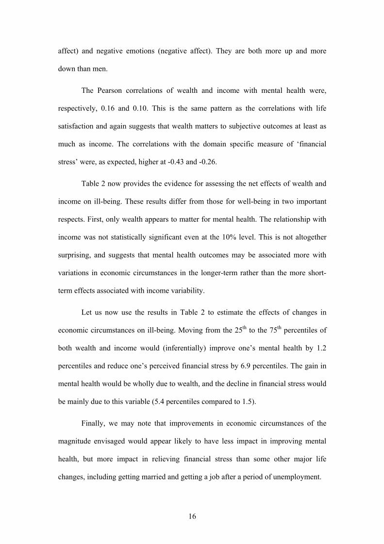
The Pearson correlations of wealth and income with mental health were,
respectively, 0.16 and 0.10. This is the same pattern as the correlations with life
satisfaction and again suggests that wealth matters to subjective outcomes at least as
much as income. The correlations with the domain specific measure of ‘financial
stress’ were, as expected, higher at -0.43 and -0.26.
Table 2 now provides the evidence for assessing the net effects of wealth and
income on ill-being. These results differ from those for well-being in two important
respects. First, only wealth appears to matter for mental health. The relationship with
income was not statistically significant even at the 10% level. This is not altogether
surprising, and suggests that mental health outcomes may be associated more with
variations in economic circumstances in the longer-term rather than the more short-
term effects associated with income variability.
Let us now use the results in Table 2 to estimate the effects of changes in
economic circumstances on ill-being. Moving from the 25th to the 75th percentiles of
both wealth and income would (inferentially) improve one’s mental health by 1.2
percentiles and reduce one’s perceived financial stress by 6.9 percentiles. The gain in
mental health would be wholly due to wealth, and the decline in financial stress would
be mainly due to this variable (5.4 percentiles compared to 1.5).
Finally, we may note that improvements in economic circumstances of the
magnitude envisaged would appear likely to have less impact in improving mental
health, but more impact in relieving financial stress than some other major life
changes, including getting married and getting a job after a period of unemployment.

17
V Discussion
This paper has shown that objective economic circumstances matter a good
deal more to well-being and ill-being or, one can loosely say, to happiness than
previously believed. Wealth (net worth) appears to matter at least as much as income,
so its inclusion changes our picture of the importance of economics to well-being.
Wealth is probably important because it provides economic security, which many
people value highly. Future work may well show that other measures of living
standards, including consumption, have significant additional effects. This is not to
claim that previous research was wrong in emphasising that personality and personal
relationships are more important to well-being and ill-being than material factors, but
the unimportance of material circumstances has been exaggerated, largely as a
consequence of omitting all variables bar income. In many cases, too, researchers
have relied on measures of pre-tax, pre-transfer income – rather than equivalized
disposable income – and so have omitted the main effects of government policy in
redistributing income and potentially redistributing well-being and ill-being.
Arguably, our results have implications both for the psychology literature on
happiness and for welfare economics. The implications for psychology are obvious
and just involve a modified understanding of what matters to well-being and ill-being.
The implications for economics are subtler. If the ‘revealed preferences’ approach
survives the challenges it currently faces, then research on happiness will presumably
remain on the fringe of economics. If, on the other hand, it comes to be accepted by
increasing numbers of economists that gains in utility cannot be validly inferred from
18
gains in consumption and leisure, then issues will arise about the direct measurement
of utility/happiness. It will then be comforting to know that household living
standards – and therefore, by inference, national economic growth – matter quite
substantially to utility/happiness.
19
REFERENCES
Andrews, F.M. and Withey, S.B. (1976), Social Indicators of Well-being: Americans’
Perceptions of Quality of Life, Plenum Press, New York.
Argyle, M. (1987), The Psychology of Happiness, Routledge, London.
Bradburn, N.M. (1969), The Structure of Psychological Well-Being, Aldine, Chicago.
Buhmann, B., Rainwater, L. Schmaus, G. and Smeeding, T.N. (1988), ‘Equivalence
Scales, Well-being, Inequality and Poverty: Sensitivity Estimates Across Ten
Countries, Using the Luxembourg Income Study (LIS) Database’, The Review of
Income and Wealth, 34, 115-42.
Campbell, A., Converse, P.E. and Rodgers, W.L. (1976), The Quality of American
Life: Perceptions, Evaluations, and Satisfactions, Russell Sage Foundation, New
York.
Diener, E. (1984), ‘Subjective Well-being’, Psychological Bulletin, 95, 542-575.
Diener, E., Suh, E.M., Lucas, R.E. and Smith, H.L. (1999), ‘Subjective Well-being:
Three Decades of Progress’, Psychological Bulletin, 125, 276-302.
Diener, E. and Biswas-Diener, R. (2002), ‘Will Money Increase Subjective Well-
being? A Literature Review and Guide to Needed Research’, Social Indicators
Research, 57, 119-169.
Duesenberry, J.S. (1949), Income, Saving and the Theory of Consumer Behavior,
Harvard University Press, Cambridge.
Frank, R.H. (1985), ‘The Demand for Unobservable and Other Nonpositional Goods’,
American Economic Review, 75, 101-16.

20
Frey, B.S. and Stutzer, A. (2002), ‘What Can Economists Learn From Happiness
Research?’ Journal of Economic Literature, 40, 402-435.
Easterlin, R.A. (1974), ‘Does Economic Growth Improve the Human Lot? Some
Empirical Evidence’, in: P.A. David and M.W. Reder (eds), Nations and
Households in Economic Growth: Essays in Honor of Moses Abramowitz,
Academic Press, New York: 89-125.
Goodin, R.E., Headey, B.W., Muffels, R. and Dirven, H-J. (1999), The Real Worlds of
Welfare Capitalism, Cambridge University Press, Cambridge.
Headey, B.W., Kelley, J. and Wearing, A.J. (1993), ‘Dimensions of Mental Health:
Life Satisfaction, Positive Affect, Anxiety and Depression’, Social Indicators
Research, 29, 63-83.
Headey, B.W., Marks, G. and Wooden, M. (forthcoming), ‘The Structure of
Household Wealth in Australia’, Melbourne Institute Working Paper Series,
Melbourne Institute of Applied Economic and Social Research Working Paper
Series, University of Melbourne.
Headey, B.W. and Wearing, A.J. (1992), Understanding Happiness, Longman
Cheshire, Melbourne.
Henderson, S., Byrne, D.G. and Duncan-Jones, P. (1981), Neurosis and the Social
Environment, Academic Press, New York.
Hollaender, H. (2001), ‘On the Validity of Utility Statements: Standard Theory
Versus Duesenberry’s’, Journal of Economic Behavior and Organization, 45,
227-49.
Juster, F.T., Smith, J.P. and Stafford, F. (1999), ‘The Measurement and Structure of
Household Wealth’, Labour Economics, 6, 253-276.

21
Kahnemann D., Diener, E. and Schwarz, N. (1999), Well-Being: The Foundations of
Hedonic Psychology, Russell Sage Foundation, New York.
Mullis, R.J. (1992), ‘Measures of Economic Well-being as Predictors of
Psychological Well-being’, Social Indicators Research, 26, 119-135.
Samuelson, P.A. (1938), ‘A Note on the Pure Theory of Consumer’s Behavior’,
Economica, 5, 61-71.
Shields, M. and Wooden, M. (2002), ‘Investigating the Role of Neighbourhood
Characteristics in Determining Life Satisfaction’, Melbourne Institute Working
Paper Series no. 24/03, Melbourne Institute of Applied Economic and Social
Research, University of Melbourne.
Watson, N. and Wooden, M. (2002), ‘The Household, Income and Labour Dynamics
in Australia (HILDA) Survey: Wave 1 Survey Methodology’, HILDA Project
Technical Paper Series no. 1/02, May, Melbourne Institute of Applied Economic
and Social Research, University of Melbourne.
22
TABLE 1
Impact of Wealth and Income on Well-Being: OLS Regressions (robust standard errors in parentheses)
Explanatory variables Life satisfactiona Financial satisfactiona
Equivalized income (/1000) .04 [β=.05]*** (.01)
.14 [β=.13]*** (.01)
Log net worth .57 [β =.07]***(.14)
2.96 [β=.22]*** (.21)
Sex (f=1, m=0) .93** (0.35)
.47 (.51)
Age -1.23*** (0.17)
-1.62*** (.25)
Age squared (/10) .02*** (.002)
.02*** (.003)
Partnered 5.52*** (.45)
3.34*** (.63)
Educational attainment Tertiary degree -.10
(.62) 3.24*** (.90)
Trade qualification 1.18* (.60)
.36 (.86)
Less than 12 years schooling 2.78*** (.66)
1.07 (.95)
Employment status Employed -.39
(.53) 3.85*** (.77)
Unemployed -3.90** (1.29)
-11.33*** (1.71)
Disability status Severe disability -15.38***
(3.42) -10.94** (3.55)
Moderate disability -6.15*** (0.68)
-6.59*** (.89)
Mild disability -2.61*** (0.81)
-3.57** (1.14)
R squared (adjusted) 0.081 0.175 Model F 37.02*** 94.29*** Breusch-Pagan 430.76*** 261.03*** Ramsey RESET 2.10 38.69*** N 7934 7931 Notes: a. Metric coefficients are shown for all explanatory variables. For income and wealth
standardized coefficients [βs] are also given to assist comparisons of the relative importance of wealth and income as determinants of well-being.
*** significant at .001 level; ** significant at .01; *significant at .05; ns = not significant. The reference variable for education was ‘completed year 12’ and the reference variable for
employment status was ‘not in the labour force’. For disability status the reference is ‘no disability’.

23
TABLE 2 Impact of Wealth and Income on Ill-Being:
OLS Regressions (robust standard errors in parentheses)
Explanatory variables Mental healtha Financial stressa
Equivalized income (/1000) .01 [β=.01] (.01)
-.06 [β=-.08]***(.01)
Log net worth .61 [β =.06]***(.15)
-2.99 [β=-.31]***(.18)
Sex (f=1, m=0) -1.87*** (0.41)
.31 (.36)
Age -.91*** (0.20)
.69*** (.18)
Age squared (/10) .01*** (.002)
-.01*** (.002)
Partnered 2.74*** (.51)
-3.08*** (.50)
Educational attainment Tertiary degree .05
(.73) -1.30* (.64)
Trade qualification .33 (.70)
.89 (.64)
Less than 12 years schooling -.35 (.75)
1.34 (.69)
Employment status Employed 3.46***
(.60) -3.08*** (.58)
Unemployed -1.08 (1.35)
6.37*** (1.56)
Disability status Severe disability -18.35***
(3.11) 1.58
(2.52) Moderate disability -12.23***
(.77) 5.41*** (.75)
Mild disability -3.79*** (.91)
.43 (.75)
R squared (adjusted) 0.109 0.236 Model F 44.70*** 93.56*** Breusch-Pagan 260.54*** 1781.21*** Ramsey RESET 5.11** 62.27*** N 7067 7027 Notes: a. Metric coefficients are shown for all explanatory variables. For income and wealth
standardized coefficients [βs] are also given to assist comparisons of the relative importance of wealth and income as determinants of well-being.
*** significant at .001 level; ** significant at .01; *significant at .05; ns = not significant. The reference variable for education was ‘completed year 12’ and the reference variable for
employment status was ‘not in the labour force’. For disability status the reference is ‘no disability’.


![Guidelines OECD Guidelines on Measuring Subjective Well-being€¦ · OECD Guidelines on Measuring Subjective Well-being-:HSTCQE=V^V[Y]: OECD Guidelines on Measuring Subjective Well-being](https://img.pdfslide.us/doc/110x75/600dac959ab70e25e9371c99/guidelines-oecd-guidelines-on-measuring-subjective-well-oecd-guidelines-on-measuring.jpg)