THE EFFECTS OF THE INTRODUCTION OF TAX INCENTIVES … · OF THE INTRODUCTION OF TAX INCENTIVES ON RETIREMENT SAVINGS 2007 Documentos de Trabajo ... 1579-8666 (on line) Depósito legal:

Juan Ayuso, Juan F. Jimenoand Ernesto Villanueva

THE EFFECTSOF THE INTRODUCTION OF TAX INCENTIVES ON RETIREMENT SAVINGS

2007

Documentos de Trabajo N.º 0724

THE EFFECTS OF THE INTRODUCTION OF TAX INCENTIVES ON RETIREMENT

SAVINGS

THE EFFECTS OF THE INTRODUCTION OF TAX INCENTIVES

ON RETIREMENT SAVINGS

Juan Ayuso, Juan F. Jimeno y Ernesto Villanueva

BANCO DE ESPAÑA

Documentos de Trabajo. N.º 0724 2007

The Working Paper Series seeks to disseminate original research in economics and finance. All papers have been anonymously refereed. By publishing these papers, the Banco de España aims to contribute to economic analysis and, in particular, to knowledge of the Spanish economy and its international environment. The opinions and analyses in the Working Paper Series are the responsibility of the authors and, therefore, do not necessarily coincide with those of the Banco de España or the Eurosystem. The Banco de España disseminates its main reports and most of its publications via the INTERNET at the following website: http://www.bde.es. Reproduction for educational and non-commercial purposes is permitted provided that the source is acknowledged. © BANCO DE ESPAÑA, Madrid, 2007 ISSN: 0213-2710 (print) ISSN: 1579-8666 (on line) Depósito legal: M.32601-2007 Unidad de Publicaciones, Banco de España

Abstract

This paper uses a Spanish panel of tax returns and another on household expenditure during

the period 1985-1991 to examine the incidence of the introduction in 1988 of tax incentives

to retirement savings on contributions to pension funds and on savings. We first identify the

population cohorts who most used these incentives. Then we use data on the evolution of

consumption of these cohorts to find that there is substantial heterogeneity in the response

of household saving to tax incentives. Most contributions to pension funds are by older/high

income individuals. While the overall amount of new saving we estimate is limited (at most 25

cents per euro contributed on average), saving responses differ substantially across age

groups. In particular, we document very small consumption drops among the group of

households between 56 and 65 years of age, the group that most actively contributed to the

plan, while we find instead a larger decrease in consumption expenditures of the group of

households between 46 and 55 years of age.

JEL codes: D14, H24, H55.

Keywords: Pension funds, tax incentives, savings.

1 IntroductionTax incentives of retirement savings are present in many countries. They couldbe rationalized as a mean to achieve that individuals accumulate more wealthfor retirement. This could happen through two channels: i) the existence ofthese tax incentives makes individuals to save more during their working lives,and ii) they change the composition of wealth portfolios by increasing the weightof "long-run" savings, as, for instance, contributions to pension plans, which areless liquid and, thus, less likely to be used before retirement.Indeed, contributions to pension funds rise significantly with tax incentives,

particularly among individuals with age close to retirement and facing high mar-ginal tax rates, a fact that we document extensively in this paper for the Spanishcase. However, the extent to which tax incentives rise retirement savings by in-creasing the portfolio weight of "long-run" savings is debatable, as it dependson the existence of borrowing constraints that could preclude the possibility ofobtaining credit using pension wealth as collateral.Hence, the empirical literature on tax incentives on retirement savings has

focused on the first channel mentioned above, namely, their impact on savingand consumption. Whether tax incentives do indeed raise saving, rather thansimply producing a change in the composition of households’ wealth portfolios,is a controversial issue. In the empirical literature on the effectiveness of taxincentives at raising savings, there are dissenting sets of results.1 For instance,while Poterba, Venti and Wise (1995 and 1996) find that in the US funds accu-mulated in Individual Retirement Accounts (IRAs) and 401(k) plans are mostlynet additions to saving, Gale and Scholz (1994) and Engen, Gale and Scholz(1996) conclude that tax incentives of retirement savings have a strong effect onthe allocation of saving and wealth, but little or not effect on the level, and thatvirtually all of the reported increase in financial assets in IRAs can be attributedto stock market booms, higher real interest rates, and shifts in non financial as-sets, debt, pensions and Social Security’s wealth.2 Hubbard and Skinner (1996)argue that probably "the truth lies somewhere between the two extremes", asthe results seem to rely on the assumed degree of substitution between taxablesaving and saving eligible for tax incentives.3 Attanasio, Banks and Wakefield(2004) notice that new contributors to IRAs,who face higher marginal interestrates, should experiment a lower consumption growth than old contributors ifthe tax-favoured scheme is effectively rising saving. However, they find that the

1For a recent surveys of this literature, see Hawksworth (2006) or Bernheim (2002)2 In the US, there are two schemes favouring retirement savings, IRAs and 401(k) plans.

Contributions to IRAs are tax-deductible up to certain limits. Deposits in 401(k) accountsare also tax-deductible. In both cases, the return to the contributions accrues tax free andtaxes are paid upon withdrawal. Participation in IRAs is voluntary, but only employees offirms that offer them are elligible to participate in 401(k) plans. Employees’ contributionsto 401(k) plans can be "matched" by employer’s contributions and, under certain conditions,employees may borrow funds from their 401(k) accounts.

3While Poterba, Venti and Wise (1996) interpret the fact that many households do notparticipate in IRAs as indication of the imperfect substitution between IRAs-saving and tax-able saving, Engen, Gale and Scholz (1996) believe that participation arises mostly from tastefor saving.

2

BANCO DE ESPAÑA 9 DOCUMENTOS DE TRABAJO N.º 0724

stock of non-IRAs assets grows less for new contributors than for continuingcontributors, being the most likely cause that new contributors are reshufflingexisting portfolios into the IRAs, and not changing their consumption-savingdecision.4

Outside the US, there is not much evidence for other countries on this issue.5

This unsatisfying state of affairs is, to a large extent, due to three substantiveproblems that make it very difficult to identify the effects of tax incentives onsaving:i) The wide heterogeneity in the individual responses to tax incentives. The

effects of tax incentives on saving, as on the value of pension wealth, depend onmany factors, such as age, the existence of liquidity constraints, the relevanceof bequest motives, the difference between the time discount factor and ratesof return, and plausible distortionary effects on labour supply. Additionally,individual preferences for saving may change through time (beyond the changesimplied by the life-cycle model), as it may change the degree of substitutabilitybetween retirement savings and other forms of savings, including housing wealth.All these factors affect, not only to the rate of return of different assets, butalso to the degree of substitutability among them.ii) The lack of microeconomic data on consumption, saving, and wealth. Not

only the effects of tax incentives may be different across individuals, also changesin tax incentives of retirement savings typically go in hand with other changes intaxes and/or in pension wealth that also affect individuals in a different mannerdepending upon their position in the life cycle and their accumulated wealth.Hence, the identification of the effects of tax incentives on saving requires theobservation of a wide range of financial and personal characteristics determin-ing marginal tax rates, earnings volatility, pension wealth, discount and inter-est rates, etc., together with individual/household-level information on income,consumption, and wealth and its composition. Moreover, since households arelikely to have different underlying preferences for savings (substitution and in-come effects vary across individuals), the estimation of the impact of changesin tax incentives requires using panel data to control for unobserved individualcharacteristics.iii) The differential impact that tax incentives may have at the moment when

they are introduced with respect a situation in which they have been operativefor a long period. Tax incentives for retirement saving may affect both to thelevel of saving and to the composition of wealth. Typically, contributions topension funds exempted from income taxation (the usual instrument that im-plements these tax incentives) are subject to certain limits, which are morelikely to be binding at the moment when tax incentives are introduced. Thus,

4This is consistent with the large elasticities of substitution between pension wealth andpersonal savings typically found in other empirical studies (see Attanasio and Rohwedder,2003 and the references therein).

5 See Milligan (2002) and Veall (2001) on Canada, Blundell, Emerson and Wakefield (2006)and Chung, Disney, Emmerson and Wakefiled (2006) on the UK, and Japelli and Pistaferri(2002) on Italy. There is also some aggregate evidence based on cross-country regressions(e.g. Lopez-Murphy and Musalem, 2004), pointing out that the accumulation of pensionfunds increases national savings only when they are compulsory.

3


there is likely to be some gradual adjustment to the desired level of savings andto the optimal wealth composition after the introduction of tax incentives forretirement savings, and this adjustment could be different for individuals of dif-ferent characteristics and wealth. This implies that the effects of tax incentivesat the moment of its introduction are likely to be different to their effects ina situation in which they have been operative for some time, when plausiblyindividuals’ wealth composition is closer to the desired one and the limits toexempted contributions from income taxation could be less binding.In this paper we aim at providing empirical evidence on the impact of tax

incentives on saving by examining the effects of what we consider an uniqueepisode: the introduction of tax incentives of retirement in Spain in 1988. Weargue that by using the introduction of the exemption as an arguably exogenous-to-the-individual change in incentives to save, our analysis may be less affectedby problems i) and ii) than previous work. Of course by focusing on the intro-duction of the exemption, our analysis is affected by problem iii): We providelittle information about the impact of the exemption when the program has beenoperative for a long period.6 Pension funds in Spain, the financial instrumentswhere retirement savings are deposited under some fiscal favorable treatment,have similar features to post-86 IRAs in the US. Contributions to those fundswere tax-exempted for all individuals up to a generous amount (4,500 euro in1988), allowed tax-free accrual of savings but limited disposal of accumulatedfunds before retirement. Finally, upon lump-sum withdrawal after retirement,taxation depends on the form of withdrawal: if redemption takes place in alump-sum payment 40% is exempted from income taxation, if redemption is inform of annuity, then it is taxed at marginal tax rate on income. We analyze theimpact of the introduction of these tax incentives in two steps. First, we use apanel of tax returns to identifying the population cohorts who most used theseincentives. Secondly, we use a panel of household consumption to estimating theimpact of tax incentives on consumption/saving of different population groups.We think that this paper contributes to the literature on tax incentives

to save in three different ways. First, we are able to use data spanning theperiods before and after the introduction of tax-favoured retirement plans. Inthe absence of a controlled experiment, such as in Duflo et al. (2006), examiningthe evolution of savings around the introduction of the tax exemption mitigatessome of the problems in the analysis of IRAs in the US, that typically study theimpact using post-introduction trends among different groups in the population.Secondly, we focus on the impact of the introduction of the pension funds

program on household consumption, rather than on household wealth. In doingthis, we follow Attanasio and DeLeire (2002) and depart from the work sum-marized in Poterba, Venti and Wise (1996) or Engen and Gale (1996), whofocus on the impact of tax incentives to retirement saving on household wealth.

6 In a companion paper (Ayuso, Jimeno and Villanueva, 2007) we use more recent datafrom the Spanish Survey of Household Finances, which contains information on householdwealth and its composition, and on consumption, to investigate further to what extent taxincentives promote retirement savings, after these tax incentives have been operative for someperiod.

4


While household wealth is a very important outcome, household consumptionalso conveys complementary useful information. In the presence of employercontributions, household consumption is more likely to reflect how the flow ofactive household saving is affected by tax incentives than household wealth (seeChernouzhukov and Hansen, 2001). Moreover, according to the permanent in-come hypotheses, household wealth is much more affected by transitory incomechanges than household consumption (Blundell and Preston, 1998). Any analy-sis that focuses on group-specific changes in household wealth over time faces theproblem of disentangling between the impact of tax incentives and the impactof different forms of between-group income changes.7

Thirdly, we extend the techniques in Attanasio and de Leire (2002), whoinfer the impact of tax incentives on new saving by comparing the consumptionchanges of new contributors to those of old contributors. Bernheim (2002) andPoterba, Venti and Wise (1996) object that the variation associated to actualcontributions may reflect other variables (preference for present consumption,income risk, borrowing constraints, preference for liquid portfolios) rather thanthe incentive to save.8 To get around the omitted variables problem, we builda variable that summarizes the incentives to contribute. Our instrumental vari-able is the interaction between the income marginal tax rate and the age of theindividual at the time of introduction of the exemption. Individuals with higherincome marginal tax rates experiment a higher increase in post-tax returns (Mil-ligan 2001, who cites many others) and age proxies income risk and preferencefor liquid assets. We check that our variable is indeed a strong predictor ofcontributions: it was mainly filers in the top quartile of labor earnings who ex-empted contributions and, within that group, average contributions increasedmonotonically with age. Using a separate expenditure survey, we then examineif the consumption growth of broad age groups in the top income quartile, rel-ative to our control group of young households, experienced a drop around theintroduction of the exemption.Our results suggest that there is indeed substantial heterogeneity in the

contributions to pension funds and in the response of household saving to taxincentives. While the overall amount of new saving we estimate is limited (atmost 25 cents per euro contributed on average), saving responses differ substan-tially across age groups - a finding also reported in the literature on 401(k)s.9

7Also, using consumption allows comparisons of tax incentives across countries. Whilevirtually every European country has an expenditure survey, very few countries have detailedSCF or SIPP -type of household wealth surveys.

8A first objection by Bernheim (2002) is that the timing of contributions is correlatedwith saving preferences of the households, and that such differences are hard to detect usingconsumption growth - a poor indicator of intrinsic thrift according to Bernheim, Skinner andWeingberg (1997). In addition, Bernheim (2002) and Poterba, Venti and Wise (1996) alsoargue that Attanasio and De Leire’s (2002) results can be also be re-interpreted as contribu-tions of old contributors representing new saving and those of new contributors representingportfolio reshuffling.

9Chernouzhoukov and Hansen (2004) document small wealth responses to 401(k)s in thetop of the wealth distribution and some evidence of new saving at the bottom. Engen andGale (2000) compare trends in household wealth across individuals that are not eligible forthe 401(k)s and those that are not, and document substantial heterogeneity across income

5


In particular, we document very small consumption drops among the groupof households between 56 and 65 years of age, the group that most activelycontributed to the plan. We document a larger decrease in consumption ex-penditures of the group of households between 46 and 55 years of age. A wayof interpreting such pattern of responses is that households in the verge of re-tirement find pension funds and other saving forms as strong substitutes, andtend to exhaust tax-exempted contribution limits by reshuffling their wealthportfolios. Conversely, groups further away from retirement, with plausibly lessaccumulated wealth and for whom contribution limits are plausibly not binding,need to save more to take advantage of the tax incentives of retirement savings.The structure of this paper is as follows. Section 2 provides a description

of the main regulation of pension funds in Spain when tax incentives were in-troduced in 1988. Section 3 contains some theoretical discussion of the factorsdetermining the impact of the introduction of tax incentives on retirement sav-ing. Section 4 discusses the characteristics of the panel data of tax returns andof the expenditure panel used for the empirical exercise. Section 5 examines theincidence of contributions over time, while Sections 6 and 7 compare contributionsand the evolution of consumption across population cohorts in order to infertheir effects on the level of saving. Finally, Section 8 contains some concludingremarks.

2 The introduction of tax incentives of retire-ment savings in Spain

In Spain the first piece of legislation regulating private pension funds was notpassed until 1987, when the Ley de Planes y Fondos de Pensiones (formally,Ley 8/87 ) established three types of private pension plans: employment plans(planes de empleo), under which the sponsor is a non-financial firm while its em-ployees are the plan members, associate plans (planes asociados), under whichthe sponsor is some legal association and the association members are entitledto contribute to the plan, and individual plans (planes individuales), created byfinancial entities — that act as sponsors — and open to any individual who wantsto contribute.Contributions to these funds were exempted from income taxation, up to

certain limits. More concretely, contributions below the minimum of 15% oflabour income and half a million pesetas (3,005.06 euros) where directly de-ducted from the income tax base. An additional 15% of contributions beyondthis limit but below 750,000 pesetas (4,507.59 euros) was deductible from theincome tax quota. It is worth noting that up to 1987, the income tax leviedhousehold individual partners jointly. Since 1988, however, couples may decidewhether to be taxed jointly or individually. In the former case (joint incometax return) limits apply to each spouse individually, and therefore could even

and age groups.

6


double for households opting for joint income taxation.10

Upon redemption, funds were subject to income taxation at different ratesdepending upon how redemption took place. They were considered non-regularincome if received as a single payment and as a regular income when receivedin the form of annuities. In the first case, 40% of the payment was exemptedfrom taxation, while in the second case it was taxed at the marginal tax rateon income. As the income tax on non-regular income is lower than that onregular income — in order to correct the distortion created by tax rates thatincrease with income levels when multi-period income accumulates in a singleyear — redemption in the form of a single payment was, in general, much moreprevalent.11

As in this paper we focus on the effects on household consumption of the in-troduction of tax incentives of retirement saving, it is important to bear in mindthat two other important changes in household income taxation were introducedin 1988. On the one hand, income marginal tax rates were substantially mod-ified. The rate was set to zero for income below 600,000 pts (3,606.07 euros)and raised to from 8% to 25%, at that income level. The number of rates wasreduced from 34 to 16, and the maximum one was set at 56%, 10 percentagepoints less than one year before. The effects of these changes on household netincome and therefore on household consumption will heavily depend on theirpre-tax income level. Also, as commented above, in 1988 household individualpartners were allowed to decide whether to pay income taxes individually orjointly. As the income tax is highly progressive, households were both spouseshad labour income massively opted for individual taxation.12

3 Some theoretical considerationsTypically the analysis of tax incentives of retirement saving is conducted in anequivalent manner to the rise in the marginal rate of return to saving. Under thisanalysis, tax incentives increase this marginal rate of return so that the impacton saving would depend on substitution and income effects. The relative size ofthese two effects crucially depends on the prevalence of borrowing constraintsand preferences for liquid assets.To grasp some intuition about the determinants of these effects, let us con-

sider an individual with initial wealth W0. When tax incentives for retirementsavings are introduced, contributions to pension funds, f, yield a tax deduction

10Subsequent changes in the related regulation have modified these limits several times.Currently, after the changes effective as from the beginning of 2007, there is no deductibilityin the income tax quota and the limits for deductibility from the tax basis have been set atthe minimum between 30% of labour income and 10,000 euros for tax payers below 50 years,and the minimum between 50% of labour income and 12,500 euros for tax payers aged morethan 50.11 Since 2007, however, redemption funds are considered regular income irrespectively of the

form they are received.12Female labour market participation rates in Spain have traditionally been relatively low,

more so for the older population cohorts. Thus, the effects of voluntary joint income tax filingare likely to depend on the age of the household’s head..

7


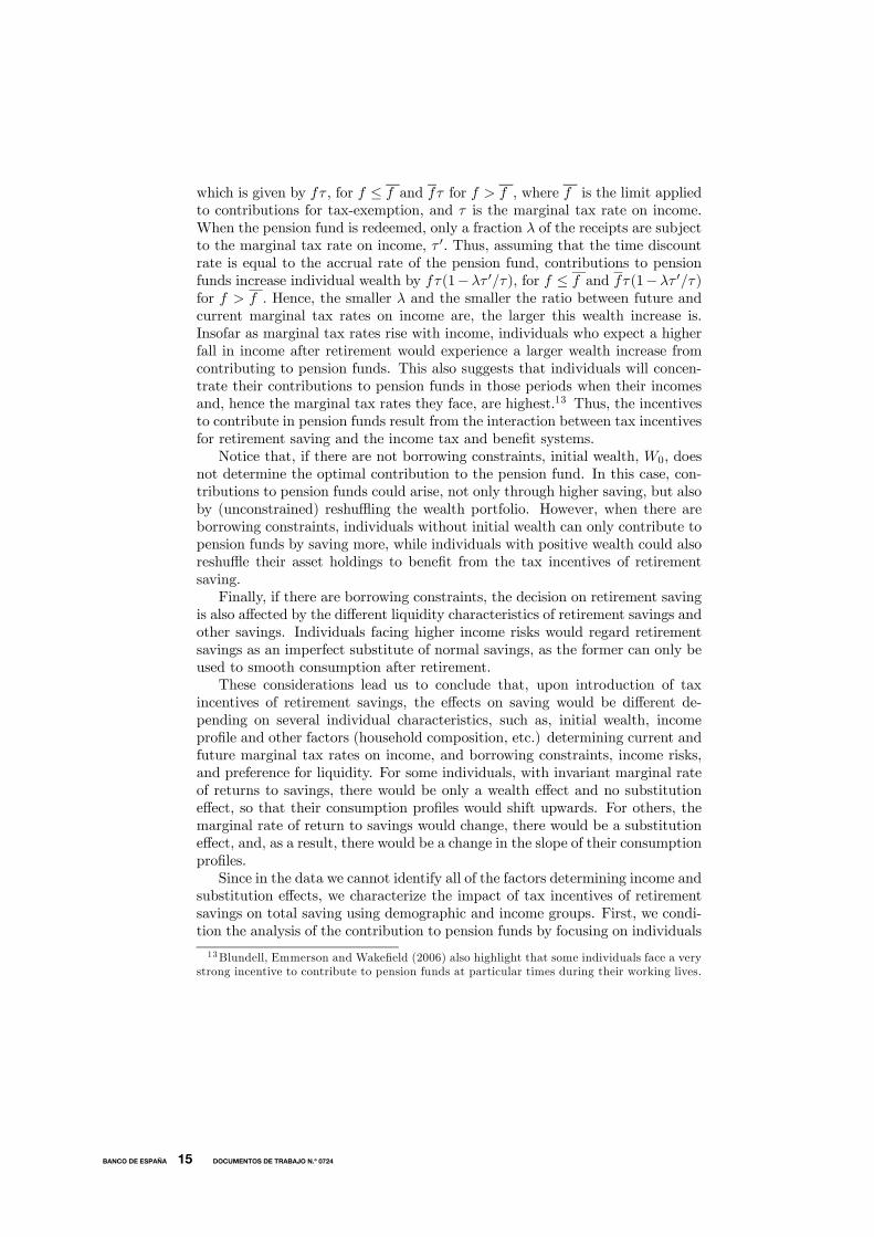
which is given by fτ , for f ≤ f and fτ for f > f , where f is the limit appliedto contributions for tax-exemption, and τ is the marginal tax rate on income.When the pension fund is redeemed, only a fraction λ of the receipts are subjectto the marginal tax rate on income, τ 0. Thus, assuming that the time discountrate is equal to the accrual rate of the pension fund, contributions to pensionfunds increase individual wealth by fτ(1−λτ 0/τ), for f ≤ f and fτ(1−λτ 0/τ)for f > f . Hence, the smaller λ and the smaller the ratio between future andcurrent marginal tax rates on income are, the larger this wealth increase is.Insofar as marginal tax rates rise with income, individuals who expect a higherfall in income after retirement would experience a larger wealth increase fromcontributing to pension funds. This also suggests that individuals will concen-trate their contributions to pension funds in those periods when their incomesand, hence the marginal tax rates they face, are highest.13 Thus, the incentivesto contribute in pension funds result from the interaction between tax incentivesfor retirement saving and the income tax and benefit systems.Notice that, if there are not borrowing constraints, initial wealth, W0, does

not determine the optimal contribution to the pension fund. In this case, con-tributions to pension funds could arise, not only through higher saving, but alsoby (unconstrained) reshuffling the wealth portfolio. However, when there areborrowing constraints, individuals without initial wealth can only contribute topension funds by saving more, while individuals with positive wealth could alsoreshuffle their asset holdings to benefit from the tax incentives of retirementsaving.Finally, if there are borrowing constraints, the decision on retirement saving

is also affected by the different liquidity characteristics of retirement savings andother savings. Individuals facing higher income risks would regard retirementsavings as an imperfect substitute of normal savings, as the former can only beused to smooth consumption after retirement.These considerations lead us to conclude that, upon introduction of tax

incentives of retirement savings, the effects on saving would be different de-pending on several individual characteristics, such as, initial wealth, incomeprofile and other factors (household composition, etc.) determining current andfuture marginal tax rates on income, and borrowing constraints, income risks,and preference for liquidity. For some individuals, with invariant marginal rateof returns to savings, there would be only a wealth effect and no substitutioneffect, so that their consumption profiles would shift upwards. For others, themarginal rate of return to savings would change, there would be a substitutioneffect, and, as a result, there would be a change in the slope of their consumptionprofiles.Since in the data we cannot identify all of the factors determining income and

substitution effects, we characterize the impact of tax incentives of retirementsavings on total saving using demographic and income groups. First, we condi-tion the analysis of the contribution to pension funds by focusing on individuals

13Blundell, Emmerson and Wakefield (2006) also highlight that some individuals face a verystrong incentive to contribute to pension funds at particular times during their working lives.

8


at the top of the income distribution, that at the time of the reform faced thehighest income marginal tax rates. We regard individuals between 20-35 yearswhen tax incentives were introduced as the most likely to have accumulated lesswealth and to find pension funds less attractive for liquidity reasons (see Galeand Scholz, 1994 for a similar reasoning). Hence, we expect contributions topension funds from these individuals to be low. We also expect contributionsto pension funds to increase with age and marginal tax rates on income. As forimpact on consumption, we expect to find a larger consumption drop amongmedium-age individuals with high income. For these individuals incentives forcontributing to pension funds are largest, as income and marginal tax rateson income are at their peaks, and uncertainty and liquidity considerations areless important than for younger individuals. Also, for this population group,accumulated wealth is not at its highest, so that reshuffling under borrowingconstraints cannot be too large, and contributions to pension funds need toarise from lower consumption. Finally for older individuals, close to retirement,wealth is higher and liquidity considerations are even less relevant, so that con-tributions to pension funds are more likely to arise from reshuffling of the wealthportfolio than from higher saving.

4 Data sets and empirical strategyWe use two data sets. The first is a micro panel of tax returns filed by individualsbetween 1982 and 1998 and collected by the Spanish Tax Agency (the so-calledPanel of Income Tax Returns). The second is a household expenditure survey.

4.1 The Panel of Income Tax Returns

In 1987 the Spanish tax authority sampled 1 in 25 tax returns in 48 out of the 52Spanish provinces, and then tracked back the returns of those filers from 1982and forward until 1998.14 To maintain the representativeness of the sample, thetax authority also added in each year after 1988 a refreshment sample with newtax returns. The introduction of the pension fund program in 1988 coincidedwith a major tax change. Before 1988, married couples had to file jointly. Afterthe tax reform in 1988 the two members of a married couple were allowed tofile separate tax returns. The 1988 reform had direct consequences both for thedesign of the sample and for the validity of our analysis. We start by discussingthe consequences for the sample, and differ the discussion on the implicationsfor our analysis to Section 6.3. Due to compulsory joint filing in the year inwhich the sample was made, the Statistical Agency was able to identify pre-1988"fiscal households" and then keep track of the tax returns filed by each memberof the original 1987 couple - even if married filers opted for filing separately ina particular year.

14Due to a special tax regime, the Basque Country and Navarra, which represent about 5%of the Spanish population, were not covered.

9


We mainly use the tax return sample to identify who contributed to pensionfunds at the onset of the program and to quantify the mean contribution bygroups. The unit of our analysis is the 1987 tax filing unit. The Panel of IncomeTax Returns contains all the information contained in a tax return (excluding allinformation that can threat anonymity). We collect the amount contributed topension funds by each tax return in the filing unit. We include both individualand employer contributions, but nothing substantially changes when we excludeemployer contributions, which represented a very small fraction of the total inthe immediate years after the introduction of the tax incentives. We also usethe yearly income of the tax filing unit and some information on householdcomposition (marital status and the number of children below 18 years of age).For 70% of the original 1987 sample, the Tax Agency also collected the age ofthe main filer. We only use the sub-sample that contains age.15

The evolution of the fraction of tax units with at least one contributor isshown in Table 1, Panel A, Column 1. While initially low, the fraction ofcontributors rapidly expanded during the 80s, and at the end of the decade some24% of tax filers had made a contribution. Possibly because contributors in 1988reported higher incomes than contributors who did their initial contributionafter that year, the mean and median contribution declined in real terms duringthe decade: from 221,873 pts. (1,337 euros in Table 1, Panel A, Column 2, firstrow, about 6% of the gross labor income reported by filers who contributed)in 1988 to 197,660 pts. (1,191 euros) in 1998 (Panel A, Column 2, last rowof Table 1), last row. As we discuss below, the vast majority of contributions(70%) were made by filing units that reported gross labor income in the topquartile of the income distribution. Contributions in the high end of the incomedistribution were relatively persistent: 81% of contributors who were in thetop income quintile in 1988 and started contributing would contribute on thefollowing year, and the average number of contributions over a six- year periodwas 5.04 (see Table A.1)We focus the analysis on the years following the introduction of the tax

exemption: 1988-1991. Panel B of Table 1 shows the summary statistics of thissub-sample. The mean gross labor income reported by the tax unit was 2,319,635pts. (13,974 euros). The (unconditional) average contribution is 10,927 pts.(65,7 euros) with 5% of tax units actually making a contribution. The meanage of the main filer is 41 years.

4.2 The Household Expenditure Survey (ECPF)

The second sample uses the 1985-1991 waves of a quarterly expenditure surveycalled Encuesta Continua de Presupuestos Familiares (henceforth, ECPF).16

The ECPF interviews some 3,000 households in each wave. Households are

15We have dropped the contributions to pension funds by tax filers who report self-employedincome, since in this case income reported could be subject to serious measurement bias.16 See Browning and Collado (2001, forthcoming), Carrasco, López-Salido and Labeaga

(2005) and Albarrán (2004) for recent uses of the ECPF to test theories of consumptionbehavior.

10


handed a notebook to record their expenses on food, transportation, textiles,health and schooling during some weeks of the quarter (see footnote 16). Also,households report retrospective information about more bulky purchases, likefurniture, cars, electronic goods (TV, and others) and white goods (washing ma-chines, dishwashers, fridges). Respondent households are tracked during eightquarters (at most), and report information about household composition andthe income received by each household member, with some disaggregation onnet-of-tax income sources. We focus on households headed by an employedindividual.The reason to focus only on a few waves is that one should only observe a

consumption drop when households start contributing and presumably adjusttheir savings plan in response to the introduction of tax incentives. After thatinitial period, the life-cycle hypothesis predicts that, holding other variablesconstant, individuals who face higher interest rates tend to delay consumptionto the future.17 Thus, we use the period up to 1991, when we observe more newfilers starting to contribute (see Table 1, Panel A, first column).Ideally , the key variables in our analysis would be total household expendi-

tures and the household-specific marginal taxes to labor income. However, whilewe make limited use of income marginal tax rates, not directly observed in thissurvey, most of our analysis focuses on pre-tax income, and concentrate on thetop two quartiles of the labor income distribution. We obtained yearly pre-taxincome by applying the withholding tax rates and adding contributions to thepost-tax income reported in the ECPF (See Appendices 1 and 2 for details).Regarding household expenditures, we have little priors on how specific house-hold consumption components react to changes in tax incentives. Thus, andfollowing Attanasio and Brugiavini (2003), we include basically all consumptioncomponents (including the expenditure in all durable goods, but housing) andpresent results separately by type of good. The main characteristics of the sub-samples are shown in Tables 2A (all households ) and 2B (the top two quartilesof the income distribution).

4.3 Empirical strategy

The empirical analysis proceeds in three steps. The first verifies that gross laborearnings at the time of the introduction of the tax incentives of retirement savingare strong predictors of both the probability of contributing and of the amountcontributed to pension funds. To that end, we use the panel of tax returns.The second step builds on the previous results and examines the evolution

of mean consumption growth of the groups that, according to the panel of taxreturns, used the contributions most heavily. The data set used in this step is theExpenditure Survey. While this strategy allows us to detect consumption dropsaround the time of the introduction of the tax incentives, we cannot quantifyhow much new saving is created.

17See Attanasio and DeLeire (2002) who discuss this point in detail.

11


Thus, in the third step we use Two-Sample Two Stage Least Squares torelate mean contributions to pension funds and mean drops in expenditure.In what follows, we discuss each of these steps in detail.

4.3.1 Distribution of contributions when tax incentives were intro-duced

Following the theoretical considerations sketched in Section 3, we examine bothcontributions to pension funds around the date of the introduction of tax incen-tives of retirement savings. As already mentioned, we expect households withhigher income marginal tax rates to experience a larger wealth effect from taxincentives and, thus, to have a higher incentive to contribute. Secondly, withinhouseholds with similar income marginal tax rates, those in the latter part oftheir working lives are most likely to contribute, as wealth is plausibly higher,and income risk and liquidity considerations are less relevant. We check thesehypotheses using the panel of tax returns to compute the average probabilityof contributing and the average contribution by age group (holding the quar-tile of labor earnings constant). We divide the sample along two dimensions:i) age groups (in four 10-years brackets), and ii) the quartile of the pre-tax la-bor earnings of the 1987 tax filing unit. This easily identifies individuals whocontributed to pension funds by most after the introduction of tax incentives ofretirement savings.

4.3.2 Changes in expenditure when tax incentives were introduced

In the second step we compare the consumption growth for individuals withhigh income marginal tax rates in the later part of their working lives (thegroup with the highest incentive to contribute) to that of individuals with highincome marginal tax rates and headed by a person below 35 years of age (thegroup with the lowest incentive). Notice that everyone who files a tax returnqualifies for the subsidy, so that a group of ineligibles does not really exist.Instead, our definition of "treatment" and "control" groups is guided by thedifferential incentive to contribute faced by households with different incomelevels.18 This test based on consumption growth has the advantage of controllingfor unobserved differences between the "control" and "treatment" group, as longas they remain constant over time. It is also unaffected by trends in saving thataffected similarly to individuals within the same income quartile or within thesame age group.19

18 In some sense, the literature on the elasticity of taxable income to marginal income taxesfaces the same problem (no one is really excluded from a change in marginal taxes, see Gruberand Saez, 2002). We borrow from that literature in defining treatment and control groups onthe basis of differences in marginal income taxes based on last year’s income.19One could argue that the right comparison is between the consumption growth of indi-

viduals who actually contribute and those who do not. Nevertheless, in using the incentiveto contribute rather than actual contributions as the key covariate we follow most of theliterature on 401(k)s. Even with complete samples, Engen and Gale (2000), Poterba, Ventiand Wise (1996) and others assess the impact of 401(k)s by comparing trends in saving be-

12


We estimate the following equation separately for the top two quartiles ofpre-tax family earnings (where the earnings quartile is determined by the firsttime we observe the household in the sample):

logCh,q+4 − logCh,q = β0 +i=3Xi=1

βi(Age_i)hPOST88q + β4POST88q +

+i=3Xi=1

(Age_i)hβ4+i + β8Xit + εh,q+4 − εh,q (1)

The dependent variable is the household-specific difference between expen-diture four quarters-ahead and current expenditure. We use a broad measureof expenditure, including durable and non durable goods.20 Age_i are threedummies indicating whether or not the household head is between 36 and 45years old, 46 and 55 years old, or 56 and 65 years old. POST88q is a dummyindicating whether or not quarter q is before or after 1987.1 (that is, if the four-periods ahead observation on expenditure happens after the introduction of theprogram). Xit contains year and quarter dummies (excluding the fourth), thelevel and 4-quarter change in household size (number of members) and compo-sition (the number ad the 4-quarter change of the number of children between1 and 2 years of age, of the number of children between 3 and 5, 6 and 13, 14and 17 and after 65 years of age). It also contains the level of gross householdearnings and the four-quarter change in household earnings. To control for thechange in reporting mode in 1988, that may have increased the expected lifetimeincome of couples by allowing separate filing, we include two extra dummies:i) an intercept of "both members of the couple work", and ii) "both memberswork" interacted with the post 88 dummy. We think that those variables cap-ture any mechanical effect of separate filing on expected lifetime income. Asfor behavioral responses, we briefly discuss them in Section 6.3. We do notinclude changes in other sources of income (like interest rates), because sav-ing in interest-yielding assets is likely to change due to the introduction of theexemption.The coefficients β1, β2 and β3 give the averages of individual changes in

expenditure growth in a specific demographic group relative to the "base" group.Those averages mix households that contribute to pension funds and those thatdo not. Note that only contributors faced a positive wealth effect at the time ofthe introduction of the program. If contributions were financed from changes in

havior between households eligible and non-eligible for 401(k) and disregard the comparisonbetween contributors and non-contributors. To reinforce our argument, notice that variationsin actual contributions are correlated with unobserved variables that may have a separateimpact on consumption growth beyond interest rate increases (time preference or changes inthe preferences for liquidity).20Namely, our measure includes both non-durable consumption (food, tobacco, alcohol,

leisure and health-related expenses) and lumply durable goods (furniture, textiles, childrenschooling and automobile expenses). Browning and Collado (2001) focus on the latter set ofgoods in a study of expenditure responses to sharp predictable income changes.

13


consumption we would expect β1, β2 and β3 to be negative. On the contrary, ifcontributions were financed from reshuffling assets, and not from higher saving,we would expect β1, β2 and β3 to be zero or non-negative.

21

Mean impacts on consumption changes may not be the only relevant mo-ment. The proportion of filers who contributed to pension funds between 1988and 1991 was low (see Table 1). Thus, the introduction of tax incentives is un-likely to have generated a constant impact throughout the distribution of con-sumption changes; on the contrary, it is likely to be located in specific centilesof the distribution. Secondly, our expenditure measure includes durable goods.If households delayed the purchase of a car or of new furniture to finance theircontributions, we would expect again a nonlinear impact over the distributionof expenditure changes. Thus, as a further specification check, we report quar-tile regression estimates of the impact of the interaction of age dummies andincome group on the 25th, 50th, 75th and 90th centiles of the distribution ofconsumption changes. Finally, and given that consumption growth is clearlyheteroskedastic, we tighten our estimates presenting Weighted Least Squares(WLS) estimates, weighting observations by the inverse of the absolute value ofthe residual of a consumption change equation estimated by OLS.22

4.4 Robustness check

A potential problem with model (1) is that it attributes any differential trend inexpenditure growth that happened between 1985 and 1990 in the age groups weconsider to the introduction of tax incentives of retirement saving. To control forage-specific trends, in some specifications we use as a benchmark the evolution ofconsumption of the group with incomes between the 50th and the 75th centile ofthe distribution of earnings (a group with high income levels but lower incentivesto contribute). Namely, using the subsample of households whose income is

21We compute standard errors allowing arbitrary heteroscedasticity and autocorrelationwithin observations from the same household. Bertrand, Duflo and Mullainathan (2004)argue that, under certain circumstances (positively autocorrelated dependent variable), stan-dard errors in DD applications may be artificially low. However, note that in our case, thedependent variable, changes in log consumption is negatively autocorrelated (coefficient ofgroup-specific autocorrelation: -.16), in which case the standard errors we report Bertrand etal’s concerns do not apply necessarily.22WLS does not always lead to unbiased estimators due to the difficulties in modelling

variances. To assess whether or not this is a problem, Table 4 reports both OLS and WLSestimates below, to permit informal comparisons of the differences in point estimates.

14


above the median, we estimate the following model:


γi(Age_i)hPOST88q ∗ 1(Y > Y.75)

+i=3Xi=1

γ4+i(Age_i)hPOST88q + γ8POST88q ∗ 1(Y > Y.75)

+i=3Xi=1

γ8+i(Age_i)h ∗ 1(Y > Y.75) +i=3Xi=1

γ12+i(Age_i)h

+γ16POST88q + γ171(Y > Y.75) + γ18Xit + uh,q+4 − uh,q (2)

Model (2) attributes to tax incentives any trend in the expenditure growth ofhouseholds in the later part of their working life and in the upper quartile ofthe distribution of earnings that is different from the corresponding trend in thesecond quartile of the distribution of earnings. Model (2) makes the implicitassumption that, if tax incentives of retirement saving had not been introduced,the difference in consumption growth between households in the top quartilewith ages above 45 and households below 35 would have evolved as the samedifference among households in the second-to-top income quartile.

4.4.1 The impact of contributions to pension funds on new house-hold saving

A parameter commonly used in the literature that evaluates the impact of taxincentives on retirement saving is "How much new saving does an extra euroof contributions generate"? The strategy described above cannot address thatquestion. To assess the amount of new saving generated by the tax incentives,and following Angrist and Krueger (1992), we combine moments from the twosamples using 2SLS estimates.Namely, we are interested in the parameter α1 of the following relationship:

Cit = α0 + α1Contrit + α2Xit + εit (3)

where Cit measures yearly consumption, Contrit is the amount contributed topension funds and Xit are covariates that include time effects, age effects andother variables. Most likely, Contrit is correlated with εit because householdsthat contribute would have had a different consumption level even in the absenceof contributions than other households, due to heterogeneity in preferences forpresent consumption and for liquid portfolios.Thus, we instrument Contrit with our identifying variable: an age trend that

differs with respect to the 20-35 age group that operates after 1988 (only) withinthe top income quartile. We assume that such differential trend only affectsconsumption growth through its impact on contributions to pension funds, thenis correlated with contributions but not with consumption. Thus, we estimateα1 using a two-sample instrumental variable regression. In the panel of taxreturns, we estimate

15


Contrit = δ0 +i=3Xi=1

δiAge_i+ ui

In the second sample (the consumption survey), we estimate

∆Cit = α0 + α1 dContrit + α2POST88t ++i=3Xi=1

δiAge_i+ εit

where Contrit is the OLS prediction in the sample of tax returns.23

Finally, two note of caution about the TSLS exercise. First, both samplesdiffer in their sampling methods and population coverage: The panel of taxreturns captures the rich in a much better way that the panel of expenditure.While we think that this is less of a problem for the former two steps procedure,that only involves identifying broad groups that contribute, it may be somewhatproblematic for imputing contributions within cells. Secondly, the specificationswith the level of consumption as a dependent variable are somewhat noisy,leading to imprecise estimates. For these two reasons, we emphasize less theseresults on new savings.

5 By how much did tax incentives promote con-tributions to pension funds?

Table 3 presents the size of contributions to pension funds of different popula-tion groups obtained using the 1988-1991 waves of the Panel of Tax Returns.Population groups are defined by age groups (in four 10-year brackets) and thepre-tax labor earnings of the 1987 tax filing unit. The centiles are computedusing the Expenditure Survey, to keep consistency across samples.Panel A shows the distribution of contributions in the top quartile of the

labor earnings distribution. The unconditional mean contribution IS increasingwith age; the unconditional mean contribution (Table 3, row 1 Column 1) in thelowest age group is 10,435 pts (62.72 euros); the same mean contribution in thegroup close to retirement (Table 3, row 1, column 4) is four times higher, 44,789pts. (269.2 euros ).The percentage of filing units with at least one contributorwas relatively small and also varies monotonically with age, from 6% in thegroup of filers with ages between 20 and 35 years of age to 12% in the groupbetween 56 and 65 years of age (Table 3, Panel A, row 2, columns 1 and 4,respectively).The proportion of filers exhausting the limits is roughly constant up to 56

years of age (12 percent of tax filers who contributed to pension funds in theprevious years, row 4 Panel A of Table 3). In the latter part of the workinglife, the fraction is much higher, 30% (Table 3, row 4 column 4). That findingis consistent with our prior that a substantial fraction of the contributions to

23We have also experimented predicting contributions with Tobits, and the point predictionswere virtually unchanged.

16


pension funds of filers in the later part of their working life may arise fromreshuffling wealth portfolios.Panels B and C in Table 3 present similar summary statistics for the second

quartile of the labor income distribution (Panel B) and the bottom two quartiles(Panel C). The unconditional group-specific average population fraction thatcontributed to pension fund is between 3 and 6 times smaller than in the topearnings quartile. Still, for all age groups, the fraction of contributors in theverge of retirement that exhaust the tax-exemption limit is about 30%.Overall, the evidence in Table 3 suggests that, if there is an impact of contri-

butions on household expenditure, it can mostly be found in the top quartile ofthe (gross) earnings distribution. In addition, the impact should vary with age.Of course, households in the bottom three quartiles of the income distributionmay have made substantial contributions to pension funds. Nevertheless, as agroup, we can only expect a little impact of the introduction of pension funds onthe expenditure of the bottom three quartiles of the income distribution. Thisleads us to make some use of households in the second—to-top income quartileas an additional control group.

6 Did tax incentives to retirement savings raisehouseholds’ saving rates?

This section presents the estimates of the drop in consumption expendituresaround the introduction of tax incentives of retirement savings, and relatesthem to the size of contributions to pension funds. Our empirical strategyattributes to the introduction of the exemption any differential negative trend inthe expenditure growth of prime-age and close-to-retirement households that ispresent in the top income quartile, but not in the second-to-top income quartile.Table A.2 presents our empirical strategy in diffs-in-diffs form. Each entry

in Table A.2 shows the average of household specific expenditure growth, byincome and age groups. Row 1 column 1 of table A.2 shows that, prior to theexemption, average consumption growth in the top income quartile for the 46-65age group was 6.5%, while in the group of 20-35 years of age consumption growthwas basically zero (row 2, column 1 of table A.2). After the introduction of theexemption, consumption growth in the group of 46-65 years of age dropped to1.2%, while it was 6.5% in the group of 20-35 years of age. This results in adiffs-in-diffs estimate of 12%. Row 4 in the second panel shows the change inconsumption growth for the age 46-65 age group in the second-to-top incomequartile. That group experimented an increase in expenditure growth of 5%(see row 4, column 3). In the second-to-top income quartile, households in the20-35 age group experimented an average expenditure growth of 8.4%. Thecorresponding diffs-in-diffs estimate is -3.3%, much lower than the 12% in row3, column 3.We provide further illustration of the dynamics of the effect in Figures 1

and 2. To detect if there was an age related discontinuity (starting in 1987)

17


in consumption growth, we ran year-specific OLS regressions of one-year-aheadhousehold expenditure growth on two dummies indicating whether the age ofthe head was between 46 and 65 years of age or between 36 and 45 years of age.24 Each estimate in each year measures the difference in log expenditure growthbetween households in the later part of the life-cycle and our control group ofyoung households. Figure 1 shows the estimates of the yearly age dummies forhouseholds in the top income quartile. Before the exemption (in years 1985and 1986), log-expenditure changes of groups above 36 and 45 years of age were.06 points larger than those of the 20-35 age group. Expenditure growth ofgroups above 36 became negative in 1987 and stayed so during the rest of thesample period. Figure 2 shows the corresponding estimates for households inthe second-to-top income quartile (who contributed much less to pension funds).While in this group the evolution is somewhat noisy in 1987, unlike householdsin the top income quartile, one-year ahead expenditure growth was positive bothbefore and after 1988.

6.1 D-in-D evidence

We start by examining the evolution of household expenditure among house-holds in the top quartile of the income distribution using estimates from equa-tion (1). Consumption growth of individuals between 56 and 65 years of age(relative to households between 20 and 35 years of age) is estimated to havefallen by 9.2% after the introduction of the program (row 1 column 1 of Table4). However, this estimate is very imprecise and not significantly different fromzero ( the standard error is 10.6%). The corresponding drop in consumptionexpenditure growth for the group between 46 and 55 years of age is 14.4%, sig-nificantly different from zero at the 10 percent confidence level (row 2, column1, Table 4). Finally, for the group between 36 and 45 years of age the drop inrelative consumption expenditure growth is 7.5%, which is consistent with thenotion that households cut their expenses upon the introduction of the program.Nevertheless, the results are very imprecise.Column 2 presents Weighted Least Squares (WLS) estimates that suggest

relatively similar effects, but much more precise standard errors. The impact isagain negative for all age groups and significantly different from zero at conven-tional confidence levels. The impact is not monotonic with age, and the highestimpact is located among the group with 46-55 years of age.As mentioned above, both the fact that few households had exempted con-

tributions in the early years following 1988 and the presence of durable goodsin our measure of expenditure leads us to expect that the age-specific drop inconsumption growth was not uniform. Columns 3 through 6 of Table 4 confirmthat hypothesis for the group of individuals between 46 and 55 years of age.The estimates shown in row 2, columns 3-5 of Table 4 suggest that the drops in

24The omitted group are households headed by a person between 20 and 35 years of age.To hold household composition constant, we also add as covariates one-year changes in de-mographics (changes in the number of children, elderly and overall number of householdmembers).

18


consumption growth were driven by a few large changes: the 75th-centile of theconsumption drop was 26 log points (standard error: .12) and the 90th centile(a drop of .33 log-points, with an standard error of .17 log-points).25 Converselymedian consumption growth did not change as much (19.7 log points, but thestandard error is 10.2). In other words, the average drop in expenditure is dueto the behavior of a limited set of households. For households close to retire-ment (56-65), we find a constant drop at different centiles, a finding that leadsus to suspect that the estimates in row 1, Column 1 of Table 4 may reflect othertrends. Finally, for our youngest treatment group (individuals between 36-45years of age), while the estimates are not significantly different from zero, themagnitude of the coefficients also suggests that the fall in consumption expen-diture growth was concentrated in the very high centiles (-22 log-points at the90th centile).Rows 4 through 6 of Table 4 present estimates from a similar specification

to that in Panel A, but for households with incomes between the 50th and the75th centiles. Those households faced lower marginal tax rates on income andcontributed less on average, as documented in Table 3. Thus, if the decreasesin consumption expenditure growth documented in rows 1-3 of Table 4 areindeed due to the introduction of tax incentives of retirement savings, we shouldfind lower impact of the introduction of the program on their consumptiongrowth. The point estimates in row 5 (the group between 46 and 55 years ofage) confirms that prior: the drop in consumption growth oscillates between .033(OLS specification) and .046 (WLS specification) and they are significantly lowerthan in the top quartile of the distribution of earnings. Further, the distributionof the drop in expenditure among the 46-55 age group is very different from thatin the top income quartile: the drop in consumption growth is not located atthe largest centiles of the distribution of consumption growth, but is basicallyuniform over the distribution.Rows 7 through 9 in Table 4 repeat the analysis now using the change in the

level (rather than logs) of consumption expenditures. The advantage of thatspecification is that one can readily interpret the magnitude of the consumptiondrop and informally compare it to the estimates in Table 3, to see how likely itis that the drop in consumption was indeed due to increases in contributions topension funds. The results in row 8 of Column 1 suggest that average expendi-ture among the group with ages between 46 and 55 fell by about 464 euros andthat the average drop was far from constant, but driven by a relatively smallset of households. Note that this average is much higher than the excess con-tribution of the 46-55 group with respect to the base group with ages between20 and 35: (102 euros, as it results from substracting Column 1, row 1 fromColumn 4, row 1 in Table 3).In rows 10 to 12 of Table 4, we examine the concepts of expenditure that

fall, and run a regression similar to equation (1), but in which the dependentvariable only contains the following set of durable goods: "white" durable goods25Standard errors in the quantile regression specification were computed by 200 bootstrap

replications in which the replications preserved the multiple observations of the same house-hold in each of the replication samples.

19


(purchases of fridges, dishwashers, washing machines... etc.), electronic goods(TVs, radios, CD players), cars and furniture. The results in row 11 suggestthat, among the group that most diminished expenditure (46-55 years of age),the bulk of the adjustment happened due to a drop in expenses of durable goods.Results (not shown) also suggest that the drop in the expenditure growth of non-durable goods (food, textiles, transportation, health and entertainment) after1988 was around 65 euros (standard error: 37,5 euros) among the group withages between 46 and 55 years of age and a not-significant drop of 89 euros, (stan-dard error: 428.6 euros) at the 90th centile of the distribution of consumption.The fact that most of the adjustment happened through durable expenditureraises several issues, that we discuss in Section 7. Yet, it is worth mentioningthat the fact that the adjustment occurred through durables, coupled with thepersistence of contributions (see Table A.1), gives a potential explanation of thediscrepancy between the estimated consumption drop and the average annualcontribution; households cut the stream of payments involved in the purchaseof a durable good to sustain their contributions.Overall, from Table 4 we draw four main conclusions. First, the introduc-

tion in 1988 of tax incentives of retirement savings coincided with a drop inconsumption expenditure growth among the treatment group of households be-tween 45 and 56 years of age in the top income quartile, relative to our controlgroup of households between 20 and 35 years of age. We find little evidence ofsuch an impact for households headed by individuals close to retirement age, afinding we discuss below. Secondly, the drop in both the log and in the level ofhousehold consumption expenditures is driven by a few large changes, consistentwith the notion that only a small fraction of households made contributions topension funds. Thirdly, further evidence for the differential trend among the46-55 age group between 1985 and 1991 being due to contributions to pensionfunds is the fact that the drop in expenditure was much lower within householdsin the same age group (46-55 years of age) within the second-to-the top incomequartile (that, as a group, contributed much less to pension funds in the onsetof the program). Fourthly, the evidence in the bottom part of Table 4 alsosuggests that households in the top quartile of the income distribution and whowere between 46 and 55 years of age reacted to the introduction of the programby delaying bulky expenditures.

6.2 Controlling for age-specific trends

A problem with the evidence presented in Table 4 is that we detect a drop inexpenditure growth for households that, as a group, did not contribute muchto pension funds; in particular households between 46 and 55 years of age andthose between 36 and 45 in the second-to-the top income quartile also experi-mented drops in expenditure growth around the time of the introduction of theexemption. An interpretation of that evidence is that there were other trendsthat depressed expenditure growth for those age groups and were not related tothe introduction of tax incentives of retirement saving.Table 5 presents results from using an alternative strategy to "net out" age-

20


specific trends. In Panel A, we substract the estimate of the drop in expenditurepresented in Table 4, rows 1-3. column 2 (that among households in the topquartile of the income distribution) to the corresponding drop in expenditurereported in Table 4, rows 4-6 column (2). We do this by using the triple-differences estimator in (2). We report WLS, and estimates of the expendituredrop at different centiles. The estimates are very similar to those reported inTable 4, rows 1-3, and we do not comment them in detail.Panel B of Table 5 experiments with an additional source of identification.

Our results so far use income quartiles to identify treatment and control groups.Yet, according to the theoretical discussion above, tax incentives of retirementsaving operate through the income marginal tax rate. The reason is that house-holds with higher income marginal tax rates experience a larger increase inthe return to retirement saving and consequently a stronger substitution effect.Hence, we explore if the expenditure drop after the introduction of tax incentivesis stronger among households that faced higher income marginal tax rates26 Weestimate the following model again for the top two quartiles of the distributionof earnings.


δi(Age_i)hPOST88qmtaxh

+i=3Xi=1

βi(Age_i)hmtaxh +i=3Xi=1

β3+iPOST88qmtaxh +i=3Xi=1

β9+i(Age_i)h

+β13POST88q + β14mtaxh + δ18Xit + υh,q+4 − υh,q (4)

where Age_i stands for three age group dummies: 36-45, 46-55 and 56-65. Theparameters of interest are δ1, δ2 and δ3 that measure the age-specific impact ofincome marginal tax rates on the average expenditure drop after the introduc-tion of the exemption. If higher income marginal tax rates are associated tolarger drops in consumption growth for all age groups, we should expect δ1, δ2and δ3 to be negative. The results shown in Table 5, Panel B confirm that forthe group between ages 46 and 55, higher consumption drops happened amonghouseholds with higher income marginal tax rates.

6.3 Other changes correlated with the introduction of theexemption

The exemption was introduced at the same time as a change in marginal incometaxes and tax splitting. To control for the change in marginal tax rates, wehave ran regressions very similar to (1) in the ECPF using marginal taxes as

26For each household in the sample, we computed the marginal income tax using the rulesbetween 1985 and 1988, ignoring all capital income (that is, we compute the marginal incometax on the first euro of capital income). After 1988, for each household we estimated whetherit was more tax-advantageous to file separately or jointly and, for those for whom separatefiling was optimal, we imputed to the household the highest marginal income tax of the couple.

21


the dependent variable, finding very small effects. Possibly, the reason for thisis that the new marginal taxes either affected households in the bottom of theincome distribution (excluded from our subsample) or at the very top of theincome distribution (who probably do not participate in an expenditure survey).Furthermore, we examine if our key variable that identifies the incentive

to contribute (a differential trend between 1985 and 1990 among different agegroups in the top quartile of the income distribution) is correlated with otheroutcomes, such as:1) Purchase of a house: Table A.3 shows the evolution of the probability

of purchasing a house in the ECPF before and after the 1988 reform, by agegroup. We find a sizable drop (-1.7 percent, relative to a overall statistic of 2.3percent) in the probability of doing so in our base group, perhaps indicatingthat the drop in expenditure in the 46-55 age group was not confined to "small"durables.2) Joint filing: The introduction of tax incentives of retirement savings in

1988 coincided with a major tax reform that changed compulsory joint filingto voluntary individual or joint filing. Such reform is likely to have changedthe income marginal tax rate and the taxable income of households. In otherwords, the 1988 introduction of separate filing may have affected the expectedpermanent income and consumption of different age groups. For example, ifjoint filing was specially prevalent among households headed by our controlgroup (persons between 18 and 36 years of age), the estimates in Model (1)would attribute to tax incentives what really is an income effect associated toa positive shock to labor supply. In principle, we focus on the top incomequartile, that experienced similar tax changes, but there could be a problem ifthe option of separate tax filing affected differently different age groups. Wecheck that possibility in Table A.3. Table A.3 Column 2 shows the impact ofour instrument ( a post-1988 dummy) on the probability that a tax filing unitfiles jointly. The group of tax filers headed by a person between 46 and 55years of age was 3.7% more likely to file jointly than the base group. Thus, as aconsequence of the tax reform, the 46-55 age group did not experience such anincome increase as the base group. Still, it is not clear to what extent this is aproblem. First, while the estimate is very precise, it is relatively small: less than4% with respect to 64% of filers who filed jointly in that income group. Secondly,we control for changes in family income in our consumption regressions shownin Table 4, for an indicator of whether both members of the couple work andan interaction of that variable with the post 88 dummy.3) Spouse participation: While the effect estimated is large (8 percent points),

as shown in Column 3 of Table 5, it is also very imprecisely estimated and notsignificantly different from zero. In addition such drop in participation is hardto reconcile with such a tiny impact of our instrument on joint filing.While we need to work more on the confounding impact of the 1988 separate

tax filing, it is not that clear that all the impact in Tables 4 and 5 is driven bysuch reform.

22


7 How much new saving are pension funds gen-erating?

This section combines expenditure data and data from contributions to estimatehow much new saving was generated by the introduction of pension funds.The evidence in Table 4 suggest that the adjustment among the group with

ages between 46 and 55 and in the top income quartile happened through dropsin durable consumption expenditures (i.e., households delayed the purchase ofa new car or furniture to contribute to pension funds). By definition, the peri-odicity of those expenses exceeds the year, so unadjusted comparisons of annualcontributions to drops in observed expenditure with periodicity over the yearare not informative.27

We use the depreciation rates in Fraumeni (1997) to distribute among sev-eral periods the bulky expenditure in durable goods when we observe one suchpurchase in the data. Namely, whenever we observe the purchase of a durablegood, we attribute to the year of the purchase (and subsequent periods if thehousehold stays in the sample) the fraction of the purchase that is depreciated.28

Unfortunately, we can estimate neither the flow of services from durables ob-tained by households who own durables but do not make a transaction duringthe sample period nor, for households that engage in a transaction, the con-sumption of the durable goods owned prior to the purchase of a new good. Wesuspect that our measure overestimates consumption drops (basically, becausewe assign a zero to pre-purchase consumption of durable goods). Summarystatistics of those variables are shown in Table 2.Table 6 reproduces the results in Table 4, now using our corrected measure of

expenditure. The WLS results in rows 1 through 3 of Table 6 are qualitativelyconsistent with those in Table 4 but the magnitude is of course much lower(for the 46-55 group, we estimate a drop in our consumption measure of 2.8percent). For the rest of the groups, we document small and not significantlydifferent from zero drops in expenditure, once we distribute expenditures indurables among periods.The second Panel in Table 6 documents the evolution of the level of peri-

odified expenditure around the introduction of the tax incentives. The averageexpenditure drop in the 46-55 year-old group is about 72 euros, standard error:40 euros. We find positive effects for the age groups of 56-65 and 36-45.Columns 2-4 of Table 6 provide an informal assessment of the extent of new

saving by age group within the top quartile of the family earnings distribution.

27The problem would be solved with either a sufficiently long panel of household expenses orwith detailed information about the stock of durables. While the ECPF is one of the longestcomprehensive consumption data sets in Europe, it only follows households for up to 2 years.Furthermore, the ECPF contains little information about wealth stocks.28Our procedure amounts to multiplying .165 to the observed total payment for a car, .1179

to the cost of furniture, .165 to expenditures in white goods and .1833 for electronic goodslike a TV or a radio. We obtain those estimates from Fraumeni (1997), who in turn obtainsthe estimates from Hulten and Wykoff (1995). See Bover (2005) for an application to Spanishdata.

23


Column 2 presents the drop in consumption estimated in Table 6, Column 1relative to the control group, as estimated in Panel A of Table 6. In Column3, we document the unconditional average contribution by each group minusthe contribution of the control group. The estimates in Column 1 are obtainedsubstracting magnitudes in row 1 of Table 3. For example, the estimated dropin consumption in the log specification for the 36 to 45 age group (relative to20-35), is presented in row 1 of column 3, and is 48 euros. On average, the 36-45age group contributed 62 euros more than the 20-35 years of age group, yieldingan estimate of increased saving of 77 cents per euro contributed. As for thegroup between 46 and 55 years of age, they contributed 119 euros more thanthe 20-35 years of age group, and their consumption fell by 63 euros. In the46-55 year-old group, 53 cents of new saving were created per euro contributed.Possibly the most surprising result is that in row 1. The contributions of thegroup that most actively contributed (top income quartile, ages between 56and 65) represented no new saving at all and most likely came from portfolioreshuffling. In Panel B of Table 7 we present similar results using consumptiondrop in levels as the dependent variable.A more formal, but perhaps less informative way of summarizing the degree

of new saving created by the pension funds program is to look at two-sampleTwo Stage Least Squares.29 Those estimates are presented in Table 7. Thefirst column in panel A is the first-stage equation, that predicts contributions topension funds using the age group of the main filer at the time of the introductionof tax incentives, and restricting taxpayers to those who were in the top of theincome distribution that year. The age dummies in column 1, Panel A, rows 2-4are significantly different from zero at any conventional significance level. TheTSLS estimate is presented in the second column of Table 7, panel A, row 1, andis .047 (.20). While extremely imprecise, results suggests that each additionaleuro of contributions does not reduce average consumption. Columns (3) and (4)include an additional control variable: dummies indicating the income bracketthe household belongs to. the rationale is to make predictions for groups thathave similar income in both samples.30 Row 2 of panel A is -.013 and suggests

29Namely, we use the following procedure. We use the subsample of hosueholds in the panelof tax returns who report incomes in the top quartile of the ECPF distribution of pre-tax earn-ings. We regress contributions (including zeroes) on the following variables: age dummies, yeardummies, a dummy the level of pre-tax household earnings, household composition variables(dummies for one, two, three and more than four descendants, a dummy for the presence ofan elderly of more than 65 years of age and the total number of members). We also includeone year-change in all variables but age. We use OLS to predict average contributions, butaverage predictions of contributions do not change much when we use a Tobit model to obtainpredictions. We then use the imputed contribution in an OLS regression of the change in thelevel of consumption on the same set of covariates listed above. Note that we identify themodel by not including in the consumption regression an interaction between age group andpost 88 dummy. Two final notes regarding the computation of the standard errors. We haveused weighted least squares to estimate the models in Table 7, where the observation-specificweights come from the inverse of the OLS residuals. Alternative weighting schemes like usingthe inverse of the household-specific standard deviation in OLS residuals did not change muchthe results. Standard errors are corrected for heteroscedasticity and arbitrary autocorrelationbetween the observations of the same household, but not for generated regressors.30The brackets included as regressors are, income between 15,000 and 18,000 euro, another

24


a 1 cent drop in consumption per euro contributed.Panel b in table 7 shows TSLS results using the top two quartiles of the

ECPF distribution of earnings. The omitted variable is the interaction betweenage group, a post 88 dummy and a dummy for top income quartile. the estimatein table 7, panel b, rows 1 is -25 cents, suggesting a larger consumption dropthan the diffs-in-diffs estimate in panel A.As we discuss above, those average estimates conceal substantial heterogene-

ity across age groups.

8 Concluding RemarksTax incentives of retirement savings might increase wealth upon retirement byeither increasing savings during individuals working lives or by changing thecomposition of wealth portfolios towards assets that are more likely to be main-tained until retirement age, as it is the case of pension funds. The identificationof the global effects of tax incentives of retirement saving is blurred by severaldifficulties, such as the wide heterogeneity in the individual responses, the lack ofmicroeconomic data on consumption, saving, and wealth through the life cycle,and the differential impact that tax incentives may have at the moment whenthey are introduced with respect a situation in which they have been operativefor a long period.In this paper we have examined the effects tax incentives of retirement sav-

ings in Spain at the period in which they were first introduced. Thus, by usingdata spanning the periods before and after the introduction of tax-favouredretirement plans, we can observe changes in consumption trends among differ-ent groups in the population which could be related to contributions to pensionfunds. For establishing this relationship, we mostly rely on the fact that individ-uals with higher income marginal tax rates experiment a higher wealth effectfrom the introduction of tax incentives, while we use age as proxy for income riskand preference for liquid assets, another dimension in which retirement savingsdiffers from other savings.While the overall amount of new saving we estimate is limited (at most

25 cents per euro contributed on average), saving responses differ substantiallyacross age groups. In particular, we document very small consumption dropsamong the group of households between 56 and 65 years of age, the group thatmost actively contributed to the plan, while we find instead a larger decrease inconsumption expenditures of the group of households between 46 and 55 yearsof age. In our view, these results cast doubts about the effectiveness of thesetax incentives to promote retirement savings, specially when compared to thefiscal costs that they have in terms of lost government revenues. Nevertheless, afull assessment of these incentives would require the measurement on its impacton wealth upon retirement, a task which is in our agenda for future work.

one for between 18,000 and 24,000 euro, another one for income between 24,000 and 30,000euro and a final one for households whose income is above 30,000 euro.

25


9 Appendix 1: ECPF Sample constructionWe use a sample of 148,679 households-quarters headed by a married ECPF re-spondents between 1985 and 1996. We exclude 2,228 observations of householdsthat reported zero food expenses at home. We also excluded 87,795 observa-tions of households whose reported income was either missing or who reportedmonthly net earnings below the statutory minimum wage. 352 observations onhouseholds-quarters headed by a retired individual were excluded. 1,227 ob-servations in which the head is unemployed were also dropped (the 19/1987law did not allow those individuals to contribute to a pension fund). We alsodropped 3116 observations of households who reported self-employment income(including farm income). We dropped further 104 cases in which the head of thehousehold was not below 65 or above 20 years of age. 21,471 observations onindividuals after 1991 were also dropped. Those restrictions left us with 27,795cases, that we used to compute year-specific quartiles of the pre-tax earningsdistribution (see Appendix 2). We could define 4-quarters ahead differencesin household expenditure for 8,376 cases. 103 cases exhibited expenditure inquarter q+4 that exceeded (were below) by more (less) than 7.38 (0.11) timesexpenditure in quarter q. We dropped such cases. Overall, we have informationon 8,273 cases (Table 2).

10 Appendix 2: Constructing pre-tax earningsin the ECPF

The paper uses pre-tax income group to split the sample. There are two reasonsfor doing this: the tax return sample provides pre-tax labor earnings and thereis a clear link between pre-tax earnings and marginal income taxes (the variablein turn determines the incentive to use a tax-favored product). However, theECPF questionnaire asks for a measure of monthly post-tax labor income (grossincome net of contributions to the Social Security System and income tax with-holdings). The ECPF staff converts the monthly report into a quarterly one.We constructed measures of pre-tax earnings out of the ECPF labor incomemeasure using four steps:Step 1: First, we annualize the quarterly net income report contained in

the ECPF. We do this by adding up all the net labor earnings we observefor the individual for each year if the individual is surveyed for four quarters.Otherwise, we convert quarterly income into yearly income by multiplying bythe corresponding factor (e.g. 4/3 if the individual is observed in 3 quarters ofthe calendar year, 2 if the individual is observed in two quarters of the calendaryear and 4 if the individual is only observed once in a year).Step 2: Each year in the sample period, the Spanish law defined a schedule

of some 27 brackets of pre-tax earnings ygross(i), where i indexes the bracketnumber=1,...,27. The schedule varies with the marital status of the individualand the number of children (if any). There are two deductions out of individualgross income: tax withholdings and social security contributions. First, when

26


gross earnings are between ygross(i − 1) and ygross(i) and exceed a minimumamount ymin_with, employers withhold a fraction of earnings tinc(i). In addition,a fraction of compulsory contributions to Social Security (typically 6% duringthe sample period) is substracted from pre-tax earnings if they lie betweena minimum level of earnings ymin_SS and ymax_SS . Using those rules, onecan define for each value of gross earnings in the grid ygross(i) a one-to-onecorresponding value of "net" earnings ynet(i).Step 3: We start the following recursion: if post-tax labor earnings ynet falls

below ymin_SS , we compute gross earnings as ynet + .06ymin_SS (during thesample period, ymin_SS was below the amount that required employers to with-hold taxes). We impute ynet

1−.06 as gross labor earnings ifynet1−.06 is above ymin_SS

but below the amount that requires employers to withhold taxes ymin_with.For values of net earnings that correspond to a level of pre-tax earnings thatrequire employees to withhold taxes, the imputed amount of gross earnings isynet−y(i)∗tinc(i−1)+y(i)∗tinc(i)

1−.06−tinc(i)We do the previous steps for each household member reporting employee

labor earnings and then compute household pre-tax earnings as the sum of theearnings of the primary and secondary earners (if one exist).A set of STATA programs and files with the mapping between gross and net

earnings is available from the authors upon request.

27


References[1] ALBARRÁN, P. (2004). The Econometrics of Income Dynamics and Ro-

tating Panels, with an Application to Precautionary Saving, mimeograph,Universidad Carlos III.

[2] ANGRIST, J. D., and A. B. KRUEGER (1992). “The Effect of Age atSchool Entry on Educational Attainment: An Application of Instrumen-tal Variables with Moments from Two Samples”, Journal of the AmericanStatistical Association, 87 (418), pp. 328-336.

[3] ATTANASIO, O. P., J. BANKS and M. WAKEFIELD (2004). “Effective-ness of Tax incentives to Boost (Retirement) Saving: Theoretical Motiva-tion and Empirical Evidence”, OECD Economic Studies, 39 (2), pp. 145-172.

[4] ATTANASIO, O. P., and A. BRUGIAVINI (2003). “Social security andhouseholds’ saving”, Quarterly Journal of Economics, 118 (3), pp. 1075-1120.

[5] ATTANASIO, O. P., and T. DE LEIRE (2002). “The Effect of IndividualRetirement Accounts on Household Consumption and National Saving”,Economic Journal, vol. 112 (6), pp. 504-538.

[6] ATTANASIO, O. P., and S. ROHWEDDER (2003). “Pension Wealth andHousehold Saving: Evidence from Pension Reforms in the United King-dom”, American Economic Review, 93 (5), pp. 1499-1521.

[7] AYUSO, J., J. F. JIMENO and E. VILLANUEVA (2007). Who BenefitsFrom Tax Incentives of Retirement Saving? Cross-sectional evidence fromthe Spanish Survey of Household Finances, work in progress.

[8] BERNHEIM, D. (2002). “Taxation and Saving”, in Handbook of PublicEconomics.

[9] BERNHEIM, D., J. SKINNER and S. WEINBERG (2001). “What Ac-counts for the Variation in Retirement Saving Across US Households?”,American Economic Review, 91 (4), pp. 832-857.

[10] BERTRAND, M., E. DUFLO and S. MULLAINATHAN (2004). “HowMuch Should We Trust Differences-in-Differences Estimates?”, 119 (1), pp.249-276.

[11] BLUNDELL, R., C. EMMERSON and M. WAKEFIELD (2006). The Im-portance of Incentives in Influencing Private Retirement Saving: KnownKnowns and Known Unknowns, Working Paper 06/09, The Institute forFiscal Studies.

[12] BLUNDELL, R., and I. PRESTON (1998). “Consumption Inequality andIncome Uncertainty”, Quarterly Journal of Economics, 113, pp. 603-640.

28


[13] BOVER, O. (2005). Wealth Effects on Consumption: MicroeconometricEstimates from the Spanish Survey of Household Finances,Working PaperNo. 0522, Bank of Spain.

[14] COLLADO, M. D., and M. BROWNING (2001). “The Response of Expen-ditures to Anticipated Income Changes: Panel data Estimates”, AmericanEconomic Review, 91 (3), pp. 681-692.

[15] – (forthcoming). "Habits and Heterogeneity in Demands: a Panel DataAnalysis", Journal of Applied Econometrics.

[16] CARRASCO, R., J. D. LÓPEZ-SALIDO and J. M. LABEAGA (2005).“Consumption and Habits: Evidence from Panel Data”, Economic Journal,115, pp. 144-165.

[17] CHERNOZHUKOV, V., and C. HANSEN (2004). “The impact of 401(k)Participation on the Wealth Distribution: an Instrumental Quantile Re-gression Analysis”, Review of Economics and Statistics, 86 (3), pp. 735-751.

[18] CHUNG, W., R. DISNEY, C. EMMERSON and M. WAKEFIELD (2006).Public Policy and Retirement Saving Incentives in the UK, mimeo, Not-tingham University.

[19] DUFLO, E., W. G. GALE, J. LIEBMAN, P. ORSZAG and E. SAEZ (2006).“Saving Incentives for Low- and Medium- Income Families: Evidence froma field experiment with H&R Block”, Quarterly Journal of Economics, 121(4), pp. 1311-1346.

[20] ENGEN. E. M., and W. G. GALE (2000). The Effects of 401(k) Plans onHousehold Wealth: Differences Across Earnings Groups, NBER WorkingPaper No. 8032, Cambridge, Mass.

[21] ENGEN, E. M., W. G. GALE and J. K. SCHOLZ (1996). “The IllusoryEffects of Saving Incentives on Saving”, The Journal of Economic Perspec-tives, 10 (4), pp. 113-138.

[22] FRAUMENI, B. (1997). “The Measurement of Depreciation in teh US Na-tional Income and Product Accounts”, Survey of Current Business, July,pp. 7-23.

[23] GALE, W. G., and J. K. SCHOLZ (1994). “IRAs and Household Saving”,American Economic Review, 84 (5), pp. 1233-1260.

[24] GRUBER, J., and E. SÁEZ (2002). “The Elasticity of Taxable Income:Evidence and Implications”, Journal of Public Economics, 84, pp. 1-32.

[25] HAWKSWORTH, J. (2006). Review of research relevant to assessing theimpact of the proposed National Pension Savings Scheme on household sav-ings, Research Report No. 373, Department for Work and Pensions.

29


[26] HUBBARD, R. G., and J. S. SKINNER (1996). “Assessing the Effective-ness of Saving Incentives”, The Journal of Economic Perspectives, 10 (4),pp. 73-90.

[27] HULTEN, C. R., and F. C. WYKOFF (1995). “Introductory Remarks:Issues in the Measurement of Economic Depreciation”, Economic Inquiry,January, pp. 10-23.

[28] JAPPELLI, T., and L. PISTAFERRI (2002). “Tax Incentives and the De-mand for Life Insurance: Evidence from Italy”, Journal of Public Eco-nomics, 87, pp. 1779-1799.

[29] LÓPEZ MURPHY, P., and A. R. MUSALEM (2004). Pension Funds andNational Saving, mimeo.

[30] MILLIGAN, K. (2002). ”Tax-preferred Savings Accounts and Marginal TaxRates: Evidence on RRSP Participation”, Canadian Journal of Economics,35, pp. 436-456.

[31] POTERBA, J. M., S. F. VENTI and D. A. WISE (1995). “Do 401(k) con-tributions crowd out other personal saving?”, Journal of Public Economics,58, pp. 1-32.

[32] – (1996). “How Retirement Saving Programs Increase Saving”, The Jour-nal of Economic Perspectives, 10 (4), pp. 91-112.

[33] VEALL, M. (2001). “Did tax flattening affect RRSP contributions?”, Cana-dian Journal of Economics, 34 (1), pp. 120-131.

30


Tables and FiguresTable 1: Summary statistics of Panel of Tax Returns.

Panel A: The incidence of contributions to "pension funds" and amounts. (1) (2) (3) (4) (5) (6)

Year 1 if contributes Mean (if nonzero) Median (if nonzero) 10th perc. 90th perc.1988 0.024 1.337 0.760 0.137 3.0121989 0.036 1.197 0.679 0.127 2.8291990 0.053 1.121 0.636 0.141 2.6831991 0.073 1.174 0.609 0.149 3.0571992 0.107 1.047 0.563 0.086 2.6521993 0.128 1.081 0.572 0.091 2.8011994 0.138 1.054 0.514 0.085 2.8441995 0.162 1.130 0.564 0.082 3.0641996 0.172 1.119 0.548 0.088 2.9501997 0.210 1.117 0.561 0.095 2.8891998 0.246 1.191 0.570 0.099 3.157

Panel B: Characteristics of 1988-1991 sample

Mean Std. Dev. Min. Max.

Contribution to pension funds 0.066 0.402 0 750

Fraction who contribute 0.0535 0.225 0 1

Contribution/gross earnings 0.063 0.072 0.001 0.4(if positive)

Household taxable income 13.974 0.010 3.704 1,012

4-quarter change, yearly income 0.888 3.701 -.263 465.89

Family size 3.374 1.13 2 12(excluding adults above 18 years)Age 41.25 11.06 20 65

Sample size: 122,5311. All monetary magnitudes in 1000s of euro (constant prices of 1987)2. Sample used in Panel A: 1988-1998 Panel of Tax returns. We only include contributions made by tax units with a filer between 20 and 65 years of age that do not report self-employed incomeContributions include both employer and individual contributions, and are aggregated at the level of 1987fiscal unit (In 1987 couples had to file income taxes jointly) 3. Sample used in Panel B: All filers between 20 and 65 years who do not report self-employment orprofessional income, between 1988 and 1991. Contributions include those made by the employer, and are aggregated at the level of the 1987 fiscal unit.


Table 2A: Summary statistics, Expenditure survey (ECPF)

Mean Std. Deviation Min. Max. Mean Std. Dev. Mean Std. Dev.

Quarterly total expenditure 2.196 1.819 0.053 49.159 1.996 1.179 2.270 1.622

Quarterly expenditure -periodified 2.101 1.485 0.053 49.159 1.882 1.470 2.168 1.962

4-quarter change of level of expenditure 0.167 1.721 -47.733 27.227 0.152 1.501 0.171 1.834

4-quarter change of level of periodified 0.166 1.328 -47.603 9.357 0.118 1.108 0.180 1.446expenditure

Household pre-tax annual earnings 10.374 5.464 7.385 51.469 8.770 4.612 11.275 5.839

4-quarter change in yearly earnings 0.982 2.311 -16.868 72.892 1.028 1.927 1.085 2.564

Family size 4.2 1.3 2 11 4.224 1.324 4.182 1.275

Age 42.6 9.9 20 65 42.7 9.86 42.45 9.894

Spouse works 0.336 0.473 0 1 0.318 0.465 0.342 0.474

Marginal income tax 26.57 3.77 0 53.98 26.443 4.649 26.603 3.456

Sample size: 8273 observations on 3202 households1. All monetary magnitudes in 1000s of euro (constant prices of 1987)2. Sample selection: Households headed by a continuously married employee, between 20 and 65 years of age. We excludeobservations in which consumption was more (less) than 7.38 (.13) times consumption four quarters before.3. Periodification of expenditure is done by applying the depreciation rates in Hulten and Wykoff (1995) to purchases of new durable goodswhen a purchase is observed. See text.4. The marginal income tax is computed on the first monetary unit of capital income and depends in principle on the filing status. To impute the household's post-88 filing status, we computed for each observation the amount paid using joint and separate filing, and assigned that with the lower tax burden

1985.1-1986.4 1987.1-1990.4

BA

NC

O D

E E

SP

AÑ

A 39

DO

CU

ME

NT

OS

DE

TR

AB

AJO

N.º 0

724

Table 2B: Summary statistics, Expenditure survey (ECPF) -Top income quartileHouseholds in top income quartile.

Mean Std. Dev. Min. Max. Mean Std. Dev. Mean Std. Dev.

Quarterly total expenditure 3.195 2.251 0.191 35.246 2.844 1.827 3.312 2.364

Quarterly expenditure 3.020 1.687 0.191 14.377 2.682 1.393 3.133 1.761

4-quarter change in expenditure (levels) 0.239 2.190 -11.124 27.227 0.149 2.373 0.016 2.649

4- quarter change periodified expenditure 0.248 1.611 -9.593 9.357 0.278 1.513 0.238 1.642(levels)

Household (yearly) taxable income 16.625 5.061 7.385 51.469 16.094 5.518 16.802 4.890

4-quarter change in yearly income 1.183 3.155 -16.868 14.360 1.445 2.888 1.096 3.235

Family size 4.31 1.27 2.00 11.00 4.314 1.3669 4.306 1.234

Age 42.85 9.13 23.00 65.00 42.826 9.604 42.858 8.966

Spouse works 0.58 0.49 0.00 1.00 0.56 0.496 0.588 0.492

Marginal income tax 28.75 3.74 23.74 53.98 28.186 4.694 28.919 3.426

Sample size Sample size: 2106 observations on 882 households observed in the top quartile of the income distribution in the quarter of the interviewSee Notes to Table 4.

2106

1985.1-1987.1 1987.2-1990.4

525 1581

BA

NC

O D

E E

SP

AÑ

A 40

DO

CU

ME

NT

OS

DE

TR

AB

AJO

N.º 0

724

Table 3: Contribution to pension funds by age and income group, 1988-1991Panel A: Gross annual labor earnings in the top quantile of the ECPF.

(1) (2) (3) (4)Age 20-35 Age 36-45 Age 46-55 Age 56-65

1. Amount contributed (includes 0s) 0.063 0.125 0.181 0.2692. Percentage households that contribute 0.061 0.092 0.115 0.1213. Contribution/taxable income (if positive) 0.068 0.0647 0.071 0.1064. Exhausts limit? 0.122 0.122 0.142 0.305

Sample size [48027] [40325] [22241] [11938]Marginal income tax

Panel B: Gross annual labor earnings in the second quartile in the ECPF.

Age 20-35 Age 36-45 Age 46-55 Age 56-655. Amount contributed 0.018 0.029 0.041 0.0596. Percent contrib. 0.0314 0.041 0.047 0.0477. Contribution/income (if positive) 0.054 0.0971 0.079 0.1158. Exhausts limit? 0.084 0.105 0.136 0.268

Sample size [34540] [17291] [12190] [9471]Marginal income tax

Panel C: Gross annual labor earnings in the bottom half of the ECPF.

Age 20-35 Age 36-45 Age 46-55 Age 56-659. Amount contributed 0.007 0.029 0.020 0.02510. Percent contrib. 0.014 0.0246 0.027 0.02211. Contribution/income (if positive) 0.076 0.0971 0.198 0.13412. Exhausts limit? 0.12 0.105 0.197 0.317

Sample size [86799] [26861] [12190] [9471]Source: 1988-1991 Panel of Income Tax Returns, sample of households where main filer is an employee. All magnitudes in 1000 euros1. Each tax filing unit in 1987 (a period of compulsory joint tax filing by couples) contributes an observation per year, regardless of filing mode.2. Sample partitions were done according to the pre-tax family earnings centiles in the ECPF.3. Labor earnings are the sum of gross earnings (including tax withholdings and social security contributions) declared by the filing unit if the original tax unit in 1988 continues to file jointly and of the tax reports of the spouses in the case of separate filings.

33.4

26.56

BA

NC

O D

E E

SP

AÑ

A 41

DO

CU

ME

NT

OS

DE

TR

AB

AJO

N.º 0

724

Table 4: Changes in expenditure among groups above median income, by age group

Estimation method: OLS WLS25th Median 75th 90th

(1) (2) (3) (4) (5) (6)

1. Age 56-65 *(POST 88) -.092 -.096 -.185 -.126 -.189 -.154(.106) (.016)** (.163) (.129) (.141) (.19)

2. Age 46-55 * (POST 88) -.144 -.127 -.033 -.197 -.26 -.33(.078)* (.020)** (.11) (.102)* (.12)** (.17)**

3. Age 36-45 * (POST 88) -.075 -.077 -.034 -.115 -.051 -.22(.075) (.013)** (.095) (.088) (.12) (.150)

Sample size:

4. Age 56-65 * (POST 88) -.005 -.005 -.03 -.015 .11 -.108(.102) (.022) (.15) (.14) (.12) (.15)

5. Age 46-55 * (POST 88) -.033 -.046 -.149 -.11 .073 -.072(.079) (.021)** (.11) (.091) (.096) (.133)

6. Age 36-45 * (POST 88) -.068 -.076 -.142 -.102 .019 -.108(.079) (.02)** (.124) (.10) (.091) (.109)

Sample size:

Dependent variable: 4-quarter change in the level of expenditure7. Age 56-65* (POST 88) 0.049 .022 -.249 -.286 -.469 .326

(.397) (.061) (.347) (.293) (.414) (.828)8. Age 46-55 * (POST 88) -0.464 -.39 -.062 -0.37 -0.515 -1.623

(.322)+ (.047)** (.261) (.219)* (.38) (.62)**9. Age 36-45 * (POST 88) -0.037 -.132 -.182 -0.268 -0.147 -0.173

(.277) (.040)** (.267) (.191) (.283) (.508)

Dependent variable: 4-quarter change in bulky purchases (cars, white & electronic goods, furniture)

10. Age 56-65* (POST 88) -.021 -0.153 -0.058 -- -0.120 -0.808( .313) (.039)** (.101) (.079) (.398)**

11. Age 46-55 * (POST 88) -.467 -0.271 -0.020 -- -0.187 -0.648(.297)+ (.023)** (.061) (.105)* (.339)**

12. Age 36-45 * (POST 88) -0.023 -0.084 0.009 -- -0.071 -0.323(.230) (.020)** (.066) (.071) (.265)

+,*,** means that the estimate is different from zero at the 15, 10, 5 percent confidence level.1. Dependent variable: log[expenditure quarter (q+4)]-log [ expenditure q]. We drop 21 cases in which total expenditure in q+4 was larger (smaller) than 7.38 (.13) times expenditure in q. 2. POST 88 is a dummy that takes value 1 if the period covered by the expenditure change includesa quarter after the first quarter of 1988. Omitted age group: 20-35 years of age.3. All models include the following covariates (not shown to save space): a POST 88 dummy,dummies for Age 56-65, Age 46-55, Age 36-45, year and quarter dummies, period q family earnings,the change in earnings between q and q+4, the number and 4-quarter change of household membersthe number of children between 1 and 3, 2 and 5, 6 and 13, 14 and 17 and above 65, and the 4-quarter change a dummy for "both members of the couple work and an interactions of "both work" and post 88.4. Analytical standard errors corrected for heteroscedasticity and correlation within observations ofthe same household shown in columns 1 and 2. In columns 3-5, standard errors are bootstrapped200 times, and each of the bootstrap replication samples is clustered at the household level.

Period: 85:1-90:4

Dependent variable: 4-quarter changes in the logarithm of expenditure

2106

"Treated" group: household income above 75th centile

"Treated" group: household earnings in top quartile

Quantile regression

2186

"Control" group: household income between 50th and 75th centile


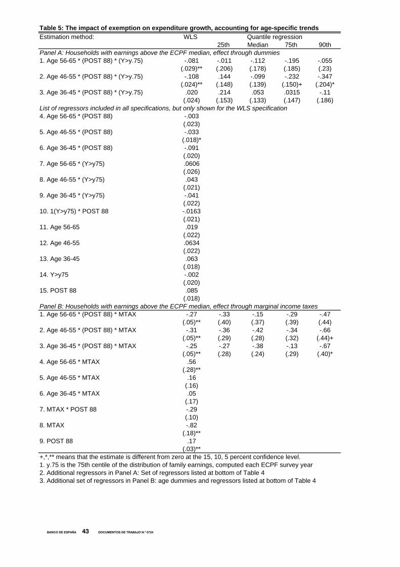
Table 5: The impact of exemption on expenditure growth, accounting for age-specific trendsEstimation method: WLS

25th Median 75th 90thPanel A: Households with earnings above the ECPF median, effect through dummies1. Age 56-65 * (POST 88) * (Y>y.75) -.081 -.011 -.112 -.195 -.055

(.029)** (.206) (.178) (.185) (.23)2. Age 46-55 * (POST 88) * (Y>y.75) -.108 .144 -.099 -.232 -.347

(.024)** (.148) (.139) (.150)+ (.204)*3. Age 36-45 * (POST 88) * (Y>y.75) .020 .214 .053 .0315 -.11

(.024) (.153) (.133) (.147) (.186)List of regressors included in all specifications, but only shown for the WLS specification4. Age 56-65 * (POST 88) -.003

(.023)5. Age 46-55 * (POST 88) -.033

(.018)*6. Age 36-45 * (POST 88) -.091

(.020)7. Age 56-65 * (Y>y75) .0606

(.026)8. Age 46-55 * (Y>y75) .043

(.021)9. Age 36-45 * (Y>y75) -.041

(.022)10. 1(Y>y75) * POST 88 -.0163

(.021)11. Age 56-65 .019

(.022)12. Age 46-55 .0634

(.022)13. Age 36-45 .063

(.018)14. Y>y75 -.002

(.020)15. POST 88 .085

(.018)Panel B: Households with earnings above the ECPF median, effect through marginal income taxes1. Age 56-65 * (POST 88) * MTAX -.27 -.33 -.15 -.29 -.47

(.05)** (.40) (.37) (.39) (.44)2. Age 46-55 * (POST 88) * MTAX -.31 -.36 -.42 -.34 -.66

(.05)** (.29) (.28) (.32) (.44)+3. Age 36-45 * (POST 88) * MTAX -.25 -.27 -.38 -.13 -.67

(.05)** (.28) (.24) (.29) (.40)*4. Age 56-65 * MTAX .56

(.28)**5. Age 46-55 * MTAX .16

(.16)6. Age 36-45 * MTAX .05

(.17)7. MTAX * POST 88 -.29

(.10)8. MTAX -.82

(.18)**9. POST 88 .17

(.03)**+,*,** means that the estimate is different from zero at the 15, 10, 5 percent confidence level.1. y.75 is the 75th centile of the distribution of family earnings, computed each ECPF survey year2. Additional regressors in Panel A: Set of regressors listed at bottom of Table 4 3. Additional set of regressors in Panel B: age dummies and regressors listed at bottom of Table 4

Quantile regression


Table 6: Changes in annualized expenditure among groups above 75th centile, by age

Estimation method: WLSDrop in expenditure Mean contribution Consumption drop

relative to relative to 18-35 age group as a fraction of18-35 age group (Table 3, row 2, differences contribution

with respect to column 1)(1) (2) (3) =(2)/(3)

1. Age 56-65 *(POST 88) 0.0166 0.033 0.207 0.159(.023)

2. Age 46-55 * (POST 88) -0.028 -0.063 0.119 -0.533(.0155)*

3. Age 36-45 * (POST 88) -0.023 -0.048 0.062 -0.772(.016)+

Panel B: Dependent variable: changes in the level of periodified expenditure

4. Age 56-65* (POST 88) 0.121 0.121 0.207 0.585(.059)**

5. Age 46-55 * (POST 88) -.072 -0.072 0.119 -0.607(.041)*

6. Age 36-45 * (POST 88) 0.120 0.120 0.062 1.708(.031)**

1. Additional regressors in Panel A: Age dummies, post 88 dummy, 4-quarter changes in demographics, log income and 4-quarter change in income, an intercept for "Both members of the couple work" and an interaction between "Both work" and "Post 88" (see bottom of Table 4)2. Column 2 in Panel A is obtained by multiplying each diffs-in-diffs estimate to the pre-exemption mean of periodified expenditureof each age group. Due to severe heteroscedasticity, we have ignored the variance of consumption growth in the computation.3. Additional regressors in Panel B: Same as in Panel A, but income changes expressed in levels (see bottom of Table 4)

Period: 85:1-90:4

Treated group: household income above 75th centile

Panel A: Dependent variable: changes in the logarithm of periodified expenditure

BA

NC

O D

E E

SP

AÑ

A 44

DO

CU

ME

NT

OS

DE

TR

AB

AJO

N.º 0

724

Table 7: The impact of an euro of contributions on annualized consumptionEstimation method: OLS Weighted TSLS OLS Weighted TSLSDependent variable: Contributions Change expenditure Contributions Change expend

(1) (2) (3) (4)Panel A: Diff-in-Diff estimates, sample of households in the top income quartile1. Contributed amount -- .047 -- -.014

(.200) (.178)2. Age 56-65*POST 88 163.98 -- 165.25 --

(13.08) (13.10)3. Age 46-55*POST 88 88.73 -- 87.87 --

(7.72) (7.61)4. Age 36-45*POST 88 27.33 -- 25.04 --

(6.19) (5.62)5. Age 56-65 --(*) 5.64 -- -20.69

(33.78) (36.94)6. Age 46-55 -- 29.54 -- 49.64

(21.38) (27.78)7. Age 36-45 -- 50.69 -- 27.84

(18.49) (21.5)8. POST 88 -27.73 -45.85

(41.09) (40.62)Level of earnings YES YESEarnings in 6000 euro brackets NO YESPanel B: Triple difference estimates, sample of households with earnings above median1. Amount contributed to PF -- -.25 -- -.25

(.204) (.207)2. Age 56-65*POST 88*1(Y>y75) 135.10 -- 136.47 --

(13.84) (13.83)3. Age 46-55*POST 88*1(Y>y75) 67.76 -- 65.55 --

(7.96) (7.73)4. Age 36-45*POST 88*1(Y>y75) 21.91 -- 17.99 --

(6.10) (5.30)5. Age 56-65*POST 88 29.02 217.19 29.45 211.81

(5.48) (30.75) (5.48) (31.5)6. Age 46-55*POST 88 22.2 46.99 23.30 21.77

(3.84) (30.60) (3.87) (26.82)7. Age 36-45*POST 88 8.08 -59.78 9.325 27.03

(2.97) (25.08) (3.00) (26.82)8. Age 56-65 * 1(Y>y75) -- 22.84 -- 12.6

(34.45) (34.55)9. Age 46-55 * 1(Y>y75) -- -14.37 -- -25.93

(24.51) (22.63)10. Age 36-45 * 1(Y>y75) -- 1.712 -- 4.1

(21.02) (20.84)11. 1(Y>y75)*POST 88 -49 -64.34 -48.68 -96.85

(14.43) (26.56) (7.49) (26.45)12. Age 56-65 -- -129.27 -- -112.52

(24.38) (28.39)13. Age 46-55 -- 19.36 -- 47.08

(27.3) (27.98)14. Age 36-45 -- 67.68 -- 64.17

(22.57) (25.59)15. POST 88 -113.82 22.57 -67.27 85.84

(23.14) (33.11) (33.46) (28.05)16 1(Y>y75) 26.6 -- 112.46

(28.68) (31.36)Level of earnings YES YESEarnings in 6000 euro brackets NO YES(*) Note that as prior to 1988, contributions were zero, covariates not interacted with POST 88 are zero


Appendix TablesTable A.1: Do contributors persist contributing?

Panel A: By occupation All employees If MTAX<28 28<=MTAX< 30 30 <=MTAX < 36 36<MTAX

Sample size: 56,831 28,333 5,767 10,281 6,853

Contributes one year after first contribution. 0.710 0.665 0.719 0.765 0.814 [median contribution] [377.71] [361.44] [433.73] [1445.8] [1237.3]

Contributes two years after first contribution. 0.654 0.596 0.629 0.717 0.778 [median contribution] [361.44] [40000] [240.96] [627.42] [1321.86]

Contributes six years after first contribution. 0.563 0.454 0.532 0.619 0.709 [median contribution] [317.86] 0 [180.72] [526.23] [1295.57]

Contributes eight years after first contribution. 0.525 0.392 0.548 0.599 0.707 [median contribution] [180.72] 0 [301.2] [526.5] [1761.9]

Average # contributions six years after 4.637 3.993 4.502 5.04 5.468

Source: Panel of tax returns (1988-1998). The sample in the second Panel only contains observations on filers who report only income as employees.C:/projects/pension_funds/panelirpf/logfiles/persistence_pf_workers1.log

BA

NC

O D

E E

SP

AÑ

A 46

DO

CU

ME

NT

OS

DE

TR

AB

AJO

N.º 0

724

Table A.2: Average 4-quarters log expenditure growth for selected groups, by age and time periodBefore 1987.1 After 1987.1 Time differences

(1) (2) (3)Panel A: Mean expenditure growth within the top income quartile1. Age 46-65 .0651 .012 -0.053

(.044) (.029) (0.041)

2. Age 20-35 -.0015 .065 0.067(.048) (.044) (.058)

D-in-D estimate3. Age difference, within period .067 -.053 -0.120

(.061) (.041) (.074)*

Panel B: Mean expenditure growth within the second-to-top income quartile4. Age 46-65 .014 .063 0.049

(.042) (.032) (.045)

5. Age 20-35 -.0174 .067 0.084(.053) (.038) (.084)

D-in-D estimate6. Age difference, within period .031 -.002 -0.0354

(.064) (.039) (.076)

1. Each entry in the Table is the group average of household specific consumption growth over four quarters. Each household contributes as manyobservations as times is observed in the sample. Standard errors clustered at the household level and computed using an OLS regression ofhousehold-specific consumption growth on age dummies, period dummies and the interactions between those variables.2. "Before 1987.1" means that the first observation used to compute household-specific expenditure growth is observed before 1987.1. Thus, consumption growthdoes not include any period after the introduction of the exemption.

BA

NC

O D

E E

SP

AÑ

A 47

DO

CU

ME

NT

OS

DE

TR

AB

AJO

N.º 0

724

Table A.3: Other changes correlated with the reformEstimation method: Probit Probit ProbitDependent variable: Purchase of a house Separate filing Spouse participationData source: ECPF Panel of Tax returns ECPFMean dependent variable 0.0237 0.649 0.42

(1) (2)1. Age 56-65 * (POST 88) -.0028 -.0015 -.0144

(.0142) (.0093) (.121)2. Age 46-55 * (POST 88) -.0153 .0375 -.085

(.0071)** (.0072)** (.097)3. Age 36-45 * (POST 88) -.0066 -.0288 .0227

(.012) (.006)** (.0967)4. Age 56-65 0.013 -0.2139

(.0182) (0.104)**5. Age 46-55 -0.0004 -0.247

(.0116) (0.089)**6. Age 36-45 0.002 -0.1896

(.0109) (0.0816)**7. POST 88 -0.012 0.048

(.011) (0.084)Sample size: 2362 106208 2082

All samples are in the top quartile of the distribution of labor earnings

BA

NC

O D

E E

SP

AÑ

A 48

DO

CU

ME

NT

OS

DE

TR

AB

AJO

N.º 0

724

Figure 1: Expenditure growth relative to 20-35, top income quartile

-0.25

-0.2

-0.15

-0.1

-0.05

0

0.05

0.1

0.15

0.2

0.25

1984 1985 1986 1987 1988 1989 1990 1991 1992

Year

Log[

C(q

+4)]-

log[

C(q

)]

Age 46-65Age 36-45

BA

NC

O D

E E

SP

AÑ

A 49

DO

CU

ME

NT

OS

DE

TR

AB

AJO

N.º 0

724

Figure 2 Expenditure growth relative to 20-35, second to top quartile

-0.25

-0.2

-0.15

-0.1

-0.05

0

0.05

0.1

0.15

0.2

0.25

1984 1985 1986 1987 1988 1989 1990 1991 1992

Year

log[

C(q

+4)]-

log[

C(q

)]

Age 46-65Age 36-45

BA

NC

O D

E E

SP

AÑ

A 50

DO

CU

ME

NT

OS

DE

TR

AB

AJO

N.º 0

724

BANCO DE ESPAÑA PUBLICATIONS

WORKING PAPERS1

0626 CRISTINA BARCELÓ: A Q-model of labour demand.

0627 JOSEP M. VILARRUBIA: Neighborhood effects in economic growth.

0628 NUNO MARTINS AND ERNESTO VILLANUEVA: Does limited access to mortgage debt explain why young adults

live with their parents?

0629 LUIS J. ÁLVAREZ AND IGNACIO HERNANDO: Competition and price adjustment in the euro area.

0630 FRANCISCO ALONSO, ROBERTO BLANCO AND GONZALO RUBIO: Option-implied preferences adjustments,

density forecasts, and the equity risk premium.

0631 JAVIER ANDRÉS, PABLO BURRIEL AND ÁNGEL ESTRADA: BEMOD: A dsge model for the Spanish economy

and the rest of the Euro area.

0632 JAMES COSTAIN AND MARCEL JANSEN: Employment fluctuations with downward wage rigidity: The role of

moral hazard.

0633 RUBÉN SEGURA-CAYUELA: Inefficient policies, inefficient institutions and trade.

0634 RICARDO GIMENO AND JUAN M. NAVE: Genetic algorithm estimation of interest rate term structure.

0635 JOSÉ MANUEL CAMPA, JOSÉ M. GONZÁLEZ-MÍNGUEZ AND MARÍA SEBASTIÁ-BARRIEL: Non-linear

adjustment of import prices in the European Union.

0636 AITOR ERCE-DOMÍNGUEZ: Using standstills to manage sovereign debt crises.

0637 ANTON NAKOV: Optimal and simple monetary policy rules with zero floor on the nominal interest rate.

0638 JOSÉ MANUEL CAMPA AND ÁNGEL GAVILÁN: Current accounts in the euro area: An intertemporal approach.

0639 FRANCISCO ALONSO, SANTIAGO FORTE AND JOSÉ MANUEL MARQUÉS: Implied default barrier in credit

default swap premia. (The Spanish original of this publication has the same number.)

0701 PRAVEEN KUJAL AND JUAN RUIZ: Cost effectiveness of R&D and strategic trade policy.

0702 MARÍA J. NIETO AND LARRY D. WALL: Preconditions for a successful implementation of supervisors’ prompt

corrective action: Is there a case for a banking standard in the EU?

0703 PHILIP VERMEULEN, DANIEL DIAS, MAARTEN DOSSCHE, ERWAN GAUTIER, IGNACIO HERNANDO,

ROBERTO SABBATINI AND HARALD STAHL: Price setting in the euro area: Some stylised facts from individual

producer price data.

0704 ROBERTO BLANCO AND FERNANDO RESTOY: Have real interest rates really fallen that much in Spain?

0705 OLYMPIA BOVER AND JUAN F. JIMENO: House prices and employment reallocation: International evidence.

0706 ENRIQUE ALBEROLA AND JOSÉ M.ª SERENA: Global financial integration, monetary policy and reserve

accumulation. Assessing the limits in emerging economies.

0707 ÁNGEL LEÓN, JAVIER MENCÍA AND ENRIQUE SENTANA: Parametric properties of semi-nonparametric

distributions, with applications to option valuation.

0708 ENRIQUE ALBEROLA AND DANIEL NAVIA: Equilibrium exchange rates in the new EU members: external

imbalances vs. real convergence.

0709 GABRIEL JIMÉNEZ AND JAVIER MENCÍA: Modelling the distribution of credit losses with observable and latent

factors.

0710 JAVIER ANDRÉS, RAFAEL DOMÉNECH AND ANTONIO FATÁS: The stabilizing role of government size.

0711 ALFREDO MARTÍN-OLIVER, VICENTE SALAS-FUMÁS AND JESÚS SAURINA: Measurement of capital stock

and input services of Spanish banks.

0712 JESÚS SAURINA AND CARLOS TRUCHARTE: An assessment of Basel II procyclicality in mortgage portfolios.

0713 JOSÉ MANUEL CAMPA AND IGNACIO HERNANDO: The reaction by industry insiders to M&As in the European

financial industry.

0714 MARIO IZQUIERDO, JUAN F. JIMENO AND JUAN A. ROJAS: On the aggregate effects of immigration in Spain.

0715 FABIO CANOVA AND LUCA SALA: Back to square one: identification issues in DSGE models.

0716 FERNANDO NIETO: The determinants of household credit in Spain.

0717 EVA ORTEGA, PABLO BURRIEL, JOSÉ LUIS FERNÁNDEZ, EVA FERRAZ AND SAMUEL HURTADO:

Actualización del modelo trimestral del Banco de España.

0718 JAVIER ANDRÉS AND FERNANDO RESTOY: Macroeconomic modelling in EMU: how relevant is the change in

regime?

1. Previously published Working Papers are listed in the Banco de España publications catalogue.

0719 FABIO CANOVA, DAVID LÓPEZ-SALIDO AND CLAUDIO MICHELACCI: The labor market effects of technology

shocks.

0720 JUAN M. RUIZ AND JOSEP M. VILARRUBIA: The wise use of dummies in gravity models: Export potentials in

the Euromed region.

0721 CLAUDIA CANALS, XAVIER GABAIX, JOSEP M. VILARRUBIA AND DAVID WEINSTEIN: Trade patterns, trade

balances and idiosyncratic shocks.

0722 MARTÍN VALLCORBA AND JAVIER DELGADO: Determinantes de la morosidad bancaria en una economía

dolarizada. El caso uruguayo.

0723 ANTON NAKOV AND ANDREA PESCATORI: Inflation-output gap trade-off with a dominant oil supplier.

0724 JUAN AYUSO, JUAN F. JIMENO AND ERNESTO VILLANUEVA: The effects of the introduction of tax incentives

on retirement savings.

Unidad de PublicacionesAlcalá, 522; 28027 Madrid

Telephone +34 91 338 6363. Fax +34 91 338 6488e-mail: [email protected]

www.bde.es

Documents

THE EFFECTS OF THE INTRODUCTION OF TAX INCENTIVES … · OF THE INTRODUCTION OF TAX INCENTIVES ON RETIREMENT SAVINGS 2007 Documentos de Trabajo ... 1579-8666 (on line) Depósito legal: