Embed Size (px)
Citation preview

1
The Effects of Regional Characteristics on Population Growth in Korean Cities, Counties and Wards*
Bun Song Lee
College of Business
Northwestern State University
306A Russell Hall
Natchitoches, LA 71497
Tel: 318-357-5324, Fax: 318-357-5990
Email: [email protected]
Sun Eae Chun
Department of Economics
Chonnam Universityu
300 Yongbong-dong, Bukku
Kwangju, Korea
Tel: 8262-530-1456, Fax: 8262-530-1559
Email: [email protected]
And
Suk Young Kim
Korea Development Institute
P.O. Box 113, Chongnyang
Seoul 130-012, Korea
Tel: 822-958-4684, Fax: 822-962-9143
Email: [email protected]
*This work was supported by Korean Research Foundation Grant(KRF-2003-042-B00033).

2
The Effects of Regional Characteristics on Population Growth in Korean Cities, Counties and Wards1
Abstract
This paper investigates the regional characteristics that influence the population growth rates in Korean cities,
counties and wards during 1980~2000. Our results indicate that regions followed the fortunes of the industries to which
regions were exposed initially. The level of education at the initial year is found to be a key determinant of region’s
population growth suggesting that higher education levels influences population growth through productivity externalities
and knowledge spillovers. The share of manufacturing employment at the initial year is found to positively affect the
population growth even though the degree of impact trends downward being consistent with the work of Glaeser et al (1995).
Our results also support the convergence hypothesis in Korea.
JEL Classification Code: R11
Keywords: Population Growth, Education, Manufacturing Industry, Fortunes of the Industries
1 The authors are grateful to three anonymous referees for their valuable suggestions.

3
1. Introduction
In parallel with the remarkable economic growth during last four decades, Korea has
experienced rapid urbanization. Development policy has been focused on the maximum utilization
of limited resources in the shortest period of time as possible exploiting the merits of agglomeration
economies. Developments of politically and geographically strategic areas were the top priority
resulting in the wide range of social, economic and cultural disparities between urban and rural areas
and among many different parts of the country. Economies of Large cities grew rapidly
experiencing rapid population growth while rural areas suffered the drastic drain of the population.
Concentration of the population and industries in large cities and in the Capital Region which includes
Seoul, Incheon and Gyunggi Province brought about various urban problems such as congestions and
pollutions.2
What are the main driving forces for the unequal population growth rates of cities in Korea?
Finding out the determinants of the city’s population growth rate and analyzing the causal relationship
of them are prerequisite for solving the unequal regional development problems in Korea. This
paper investigates these issues.
Sjaasted (1962) proposed a framework by which one can analyze the economic cost and
benefit of migration in the context of utility maximization in the long run. It is based on the neo-
classical economic theory, which views the problem of regional growth in the perspective of human
capital theory. Sjaasted regards the movement across the regions as the distribution of resources and
contends that it is the result of investment decisions of an individual who wants to increase the
productivity of the human capital. Migration investment occurs when the present value of the
expected benefit of moving is larger than the present value of the expected costs of moving.
Todaro (1969) also presents an empirical model that explains the population movement in the
context of human capital theory. In this model, population in the rural area first moves into the
informal sector of the cities, and only later moves into the modern sector after adjusting to the city
lifestyle. The movement to the cities from the rural areas is a function of the probability of
2 Gyunggi Province surrounds Seoul and Incheon is the 4th largest city in Korea located in the vicinity of Seoul.

4
employment in the cities and wage differences between urban and rural areas. Migration to the cities
is assumed to depend on the difference between the expected income to be earned while working in
the city and the real income currently earned by the worker residing in the rural area, not on the actual
real income difference between the city and the rural area.
Lowry (1966) was able to explain the 68% of the variation of migrations in metropolitan areas
(SMSA) in the United States using the gravity embedded regression model, which is based on
neoclassical economic theory in which the unemployment rates and wage rates are equalized among
the regions through the movements of workers. Workers move to the higher wage regions from the
lower wage regions and to the low unemployment regions from the high unemployment regions.
The theory also presupposes that the migration occurs in proportion to the size of the labor market
while moving inversely to the distance between the regions.
Most of the studies on the growth of cities in Korea, especially on population growth, focus on
the population concentration problem in the Capital Region of Korea which includes Seoul, Inchon,
and Gyunggi Province. There are few studies that examine the population growth of all the regions of
Korea, considering both the social and economic aspects. Lee and Kang (1989) analyzes the
relationship between the population growth and the manufacturing industry growth of cities, counties
(guns), and wards (gus) in the Capital Region in 1985. They employed variables such as population,
manufacturing related indexes, distance from Seoul, population density and volume of commuting
traffic to identify the determinants of population growth. Their findings suggest that population and
manufacturing related indexes such as number of manufacturing firms, and the values of
manufacturing product are highly correlated with each other.
The current paper investigates the entire country of Korea and search for the determinants of
the regional population growth employing comprehensive data on all the cities, counties (guns) and
wards (gus) in Korea. Various kinds of regional characteristics that are hypothesized to affect the
economic growth of cities, counties (guns), and wards (gus) are analyzed. Based on the results we
present some implications for policy with regards to the balanced development of Korea.
This paper is organized as follows. Section 2 presents the theoretical framework for our
empirical analyses. Section 3 describes the data and the regression analysis results are presented in
section 4. Section 5 concludes the paper.

5
2. Modeling Framework
Following Glaeser et. al (1995), cities will be treated as separate economies that share common
pools of labor and capital. Unlike countries, cities are completely open economies and therefore, it
is reasonable to assume the perfect mobility of capital, labor, and ideas among cities. A large
number of studies have investigated population growth across countries. However, one benefit of
analyzing population growth in cities is that cities are more specialized economic units than countries,
and hence one may gain more insight into the movements of resources and convergence across cities
than across countries.
In the context of cities, differences in urban growth experiences cannot be the result of
differences in saving rates or exogenous labor endowments. Because of the assumption of mobile
labor and capital movement, cities differ only in the ‘level of productivity’ and the ‘quality of life’.
Total output in a city is given by
σtititititi LALfAY ,,,,, )( == (1)
Where tiY , represents the total output in city i at time t, tiA , represents the level of
technology in city i at time t, tiL , denotes population of city i at time t, f(.) is a common Cobb-
Douglas production function, and σ is a parameter.3
Under perfect competition, the labor income, namely, wage rate ( tiW , ) of a potential migrant
will be equal to the marginal product of labor.
1,,,−= σσ tititi LAW (2)
3 As for nonmanufacturing sectors the data on capital stock is not avaiable. This is why equation (1) does not include capital stock variable. Therefore, we can assume that capital stock is implicitly included in both technology, tiA , and labor,
tiL , . We also assume that technology is neutral with capital stock and labor and capital stock is complement for labor.

6
Total utility for an individual in each city equals wages multiplied by a quality of life index.
Quality of life is meant to capture a wide range of factors including crimes, housing prices, and traffic
congestion.
Quality of life = δ−titi LQ ,, (3)
where δ >0. We assume that the quality of life index declines as the size of the city increases.
Total utility of a potential migrant to city i is given in (4) below and is determined by the
productivity of labor (implicitly along with capital stock) and quality of life.
Utility = 1,,,
−−δσσ tititi LQA (4)
We assume free migration across cities. This ensures constant utility level across space at a point
in time. So each individual’s utility level in different cities must equal to the reservation utility level
at time t, which we denote as 0tU
Thus, for each city:
)log()1()log()log()log(,
1,
,
1,
,
1,0
01
ti
ti
ti
ti
ti
ti
t
t
LL
AA
UU ++++ −−++= δσ (5)
We also assume that
1,',
,
1, )log( ++ += tititi
ti XA
Aεβ (6a)
1,',
,
1, )log( ++ += tititi
ti XQ
Qξθ (6b)
Where ',tiX is a vector of city characteristics at time t, which simultaneously determine the
growth in both the quality of life and the growth of technology within the city. Lastly, combining
equation (2), (5), (6a), and (6b) yields
7
1,',
,
1, )(1
1)( ++ ++
−+= titi
ti
ti XL
Lχθβ
σδlog (7)
1,',
,
1, )(1
1)log( ++ +−+
−+= titi
ti
ti XW
Wωθσθδβ
σδ (8)
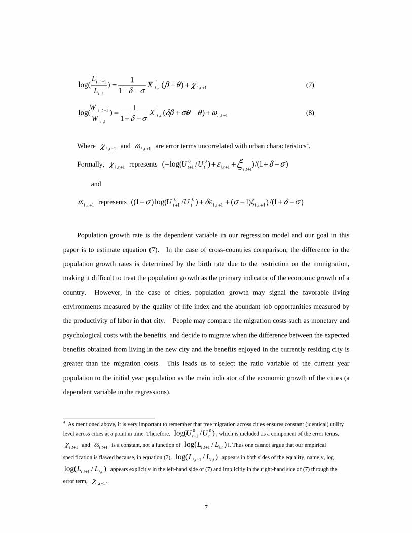
Where 1, +tiχ and 1, +tiω are error terms uncorrelated with urban characteristics4.
Formally, 1, +tiχ represents )1/())/log((1,1,
001 σδε ξ −+++−
+++ tititt UU
and
1, +tiω represents )1/())1()/log()1(( 1,1,00
1 σδξσδεσ −+−++− +++ tititt UU
Population growth rate is the dependent variable in our regression model and our goal in this
paper is to estimate equation (7). In the case of cross-countries comparison, the difference in the
population growth rates is determined by the birth rate due to the restriction on the immigration,
making it difficult to treat the population growth as the primary indicator of the economic growth of a
country. However, in the case of cities, population growth may signal the favorable living
environments measured by the quality of life index and the abundant job opportunities measured by
the productivity of labor in that city. People may compare the migration costs such as monetary and
psychological costs with the benefits, and decide to migrate when the difference between the expected
benefits obtained from living in the new city and the benefits enjoyed in the currently residing city is
greater than the migration costs. This leads us to select the ratio variable of the current year
population to the initial year population as the main indicator of the economic growth of the cities (a
dependent variable in the regressions).
4 As mentioned above, it is very important to remember that free migration across cities ensures constant (identical) utility
level across cities at a point in time. Therefore, )/log( 001 tt UU + , which is included as a component of the error terms,
1, +tiχ and 1, +tiω is a constant, not a function of )/log( ,1, titi LL + l. Thus one cannot argue that our empirical
specification is flawed because, in equation (7), )/log( ,1, titi LL + appears in both sides of the equality, namely, log
)/log( ,1, titi LL + appears explicitly in the left-hand side of (7) and implicitly in the right-hand side of (7) through the
error term, 1, +tiχ .

8
In the cross-country studies where the labor movement across countries is restricted, the income
growth (wage growth) can be interpreted as the increase in the labor productivity. However, the
situation changes when we conduct the cross-cities analysis where labor can move freely across the
cities. Migration occurs on the basis of the growth opportunities. Moreover, income (wage)
growth may reflect the compensation for the decrease of the quality of living environments as well as
reflecting productivity increases. Income growth therefore is a less clear indicator of the economic
growth of cities compared to population growth. Accordingly, equation (8) which uses wage
(income) growth as an dependent variable is not estimated in this study.
3. Data and Descriptive Statistics
This study identifies the city’s characteristics which contribute to the growth of city population
using the data on cities, counties (guns), and wards (gus) from the Korean Population Census 2%
sample tape for the five years, 1980, 1985, 1990, 1995 and 2000.
A number of new administrative units have been created during the sample periods, where some
regions were merged into a larger region horizontally or vertically, while some regions were divided
into smaller districts. In order to track down the changes in the population composition for identical
geographical regions, data are transformed in this regard.
How many are cities, wards and counties separately? 57 cities, 94 counties (guns), and 43
wards (gus) are analyzed for the long term analyses over the period of 1980-2000. The wards (gus)
in the six mega-cities (Seoul Special City, Busan, Daegu, Incheon, Gwangju, and Daejeon) are treated
separately. For the sake of convenience cities, counties (guns), and wards (gus) are called “cities”
from now on.
In order to investigate the effect of the local tax burden on the city population growth, data from
the Main Statistical Indices for Cities, Counties (guns) and Wards (gus) of 1999 are used. Per capita
local tax burden (100,000 won) in 1990 is used as one of the independent variables since it represents
the amount of the tax collected by local government.5
5 Because of the unavailability of the data, we used the data on the per capita local tax burden for 1990 (from Korea
National Statistical Office, Main Statistics for Cities, Counties (guns), and Wards (gus)of 1999) rather than data for 1980.

9
In order to investigate the effect of land-use regulations on the population growth of the city,
green belt ratio (defined as the ratio of the area in which development is restricted to the whole area of
a city) and 5 zone dummies such as “Restricted Development Subregion(RDS)”, “Controlled
Development Subregion(CDS)”, “Encouraged Development Subregion(EDS)”, “Environmental
Protection Subregion(EPS)”, and “Special Development Subregion(SDS)” in the Capital Region are
used. The greenbelt areas were designated in early 1970. The five zones were designated during
1984-1994 as a measure of “Capital Region Spatial Concentration Control Policy”. We may expect
these population concentration control policy measures would have had impact on the population
migration.
We first conduct a long-term analysis over the period 1980-2000 and then conduct sub-sample
period analyses over the sub-periods 1980-1985, 1985-1990, 1990-1995, and 1995-2000, in order to
capture the sub-sample period variations of the impact of the regional characteristics on city
population growth.
Before we look at the descriptive statistic, we have checked the nonstationarity of the data with 5
panel unit root tests such as Levin, Lin and Chu (2002), Breitung (2000), Im, Pesaran and Shin (2003),
Fisher-type tests using ADF and PP tests, following Baltagi and Kao (2000). By adding the cross-
section dimension to the time-series dimension offers an advantage in the testing for non-stationarity.
Tests such as Livin, Lin & Chu and Breitung assumes common unit root process across cross sections
while the rest of the tests assumes individual unit root process across different cross sections. Only
individual intercept is included in the specification of the model considering the simulation results of
Choi (1999a) which report decrease of the test power when a linear time trend is included in the
model. Table below shows the test results. Five panel unit root tests reject the null of unit root for
the population growth data while only Im, Pesaran and Shin rejects the null of unit root for the mean
education data. We assume all the data we use are stationary and proceed with individual regression
equation instead of focusing on the panel data set. 6
6 Panel regression has been attempted but the test resulted in the singularity problem, which is presumed to be due the
small T in our panel data set. Usually the panel data econometrics are geared to studying the asymptotics of macro panels
with large N cross section data and large T length of time series data. However, the data set we use here are typical micro
panel data set with large N with small T which is only 5.

10
<Results of Panel Unit Root Tests>
Variable Test Methods Statistic(Prob*) Cross-
sections Obs
Null: Unit root (assumes common unit root) Levin, Lin and Chu Breitung
-11.85(0.00) -5.46(0.00)
179 179
708 529
Population growth
Null: Unit root (assumes individual unit root) Im, Pesaran and Shin ADF-Fisher PP-Fisher
-16.94(0.00) 560.43(0.00) 572.37(0.00)
179 179 179
708 708 708
Null: Unit root (assumes common unit root) Levin, Lin and Chu Breitung
67.88(1.00) 47.51(1.00)
234 234
936 702
Mean Education level
Null: Unit root (assumes individual unit root) Im, Pesaran and Shin ADF-Fisher PP-Fisher
-2.11(0.02)
378.47(0.99) 26.09(1.00)
234 234 234
936 936 936
* Probabilities for Fisher tests are computed using an asymptotic Chi-square distribution. All other tests assumes
asymptotic normality
Table 1 presents means and standard deviations of the major variables used in the long-term analysis
of the 1980~2000. Average population across cities increased by 25.3% from 189,835 people in
1980 to 237,814 people in 2000. The average ratio of 2000 population to 1980 population across cities,
the log of which is the dependent variable in the regression is shown to be 1.117. The average year of
education at the initial year, 1980 was 7.28 year, while the average unemployment rate was 12% in
1980 and the per capita local tax burden in 1990 was 106,000 won.8 The average manufacturing
share in the city’s total employment was 18% in 1980. The average of the population’s average ages
7 Average of the ratios of the current year population to the initial year population is
∑=
194
1194/][
iiRATIO ,
where
it
iti pop
popRATIO
,
,1+=
and itpop , represents the total population of the city i in initial year. Therefore, it should be noted that 1.11, the average of ratios of the current year population to the initial year population across cities differs from the value obtained by dividing the average current year population across cities (237,814 people) by the average initial year population across cities(189,835 people). 8 The Korean currency unit, won, was recently valued at 1,000 won per US$1.

11
across cities is 26.219. This is the average of the average ages of each city’s population, which is
calculated by deriving the average age over the whole population in the particular city.
Table 1 also shows the shares of humanity high school graduates, business high school graduates,
junior college graduates and college graduates are 31%, 17%, 4%, and 10%, respectively. In order to
investigate the effect of the proximity to metropolitan area on city’s population growth we measure
the distance (in km) from the nearest metropolitan area, namely, the central ward of the Mega-cities or
the center of the largest city in the province. The average value of the distance is 45 km.
Table 2 shows the city’s characteristics at the initial year for the top 10 fastest growing cities and
for the bottom 10 slowest growing cities. Prominent population increases are observed in Ansan,
Ulsan, Goyang, Siheung(including Kwacheon, Kunpo, Euwang, Kwangmyung) and Bucheon. On the
other hand, the slowest growing cities observed are all counties (guns) such as Jeongseon, Sinan,
Imsil, Jian and Bonghwa.10
Fastest growing cities are those where the housing complexes in large scales were constructed
based on the Government’s development plans such as ‘Two Million Housing Project’ during 1980-
1995 and the construction of the ‘New Cities’. The Theory of ‘housing filtering process’ which
suggests that the dwelling is occupied by households with progressively lower incomes predicts that
the increase in the number of housings has a positive effect on population migration (Ha, 1991).
Whenever new housings facilities were built, the population moved into the newly built houses and
another new population moved into the old houses which the previous population had left. The fact
that the top 10 fastest population growing cities include the cities with those characteristics supports
the housing filtering process theory.
Peripheries of Seoul, such as Incheon (Bukgu including Bupyeonggu, Gyeyanggu and Seogu),
Ansan, Goyang, Siheung, Bucheon, and Suwon have experienced rapid growth since 1970.
9 The average of the population’s average ages across cities,−−AA .
∑∑
=
=−−=
194
1
1,
194/)]([i i
n
jji
n
AGEAA
i
where in is the total population of the city i and jiAGE , is the age of the jth individual of the city i 10 In Korea a county (gun) does not include any urban area, but includes rural areas only.

12
Manufacturing sector growth outside the Capital Region such as Ulsan and Changwon (top 11th fastest
population growing city with the ratio of 2000 population to 1980 population, 2.59) have been
encouraged through the factory redistribution policies in pursuit of the dispersion of the Seoul
population and balanced national land development.
Incheon attracts factories as the seaside factory park while Suwon, Siheung and Bucheon attract
factories as parks for urban-type factories. Ulsan and Changwon also have grown in population as a
result of the government’s strategy of developing the southeastern seaside region. Factory parks
were developed along the southeastern seaside around the harbor cities under the dispersion policy of
the Capital Region’s population and industry facilities. These cities emerged as the largest heavy
chemical factory parks in Korea. Growth in the manufacturing sector in these cities (Ulsan and
Changwon) is supported by the data showing high manufacturing shares (0.51 for Ulsan and 0.29 for
Changwon) in these cities as shown in Table 2.
The city’s characteristics at the initial year show the significant differences between the top 10
fastest population growing cities and bottom 10 slowest population growing cities. The average
education levels (in years) of the fastest growing cities are higher when compared to those of all cities
in the sample, and are particularly high when compared to those of the bottom 10 cities. In addition,
the manufacturing employment shares at the initial year for the top 10 cities turn out to be
significantly higher when compared to those of the lowest growing cities. The average age of the
city dwellers is found to be lower in the cities where population growth is higher.
4. Regression Results
1) Long Term Period Analysis over the Period 1980-2000
As stated above, the objective of our study is to search for the determinants of the population
growth in the cities. Table 3 reports the regression result of the effects of the city’s basic
characteristics at the initial year on the city population growth over the period 1980-2000.11 The basic
11 An anonymous referee pointed out that our regression anayses are based on the notion that the initial conditions of regional characteristics determine the future trajectory of population growth in the region. The referee criticized our paper that we ignore the dynamics of city development. To correct this problem, this referee suggested us to use simultaneous equations of population-job creation-living environment dynamics and nexus. We agree fully with this referee’s criticism

13
variables are those such as average years of education, average age of the residents, the square of the
average age, the per capita local tax burden, the unemployment rate, the manufacturing employment
share, the 1st industry employment share, the distance from the nearest metropolitan area, the ward (gu
in the mega-cities) dummy, the city dummy and regional dummies. We run four different kinds of
regression equations in Table 3 depending on our interest in the particular variables. Equation (1) is a
benchmark regression equation, whereas equation (2) especially investigates the effect of
givernment’s land use regulation and equation (3) investigates the effect of education in more detail.
Finally, equation (4) shows the results of equation (1) for the data which include six mega-cities
instead of 43 wards.
Regression results of equation (1) shows that the average education level at the initial year has a
significant positive effect on the city’s population growth.
Also it shows that the average age of the resident variable has statistically significant negative
effect on population growth, while it’s squared variable has a statistically insignificant positive effect.
City population growth requires abundant human capital to be used in production in addition to the
existence of the highly productive and prosperous industries and abundant capital stock. In the case of
Korea, the young and middle-aged population with a large amount of human capital has moved out of
rural areas, leaving the aged behind. This reduces productivity in rural areas, which reinforces the
population decline in rural areas creating a vicious circle.
Per capita local tax burden has a positive effect, but is not statistically significant. Cities with
higher tax revenue spend more on public goods such as sanitary and public facilities and therefore
cities with higher tax burden can be inferred to have a favorable living environments compared to
those cities with lower tax burden, resulting in faster population growth.
Higher unemployment rate at the initial year has a negative effect on population growth but is
not statistically significant. Unemployment rate can represent underutilized human capital. High
unemployment rate may imply lack of the skilled labor force, which is the main forces of the growth
of the city and thereby resulting in a decrease in the labor productivity. Therefore a higher
and would like to point out that dynamic issues should be our future research areas.

14
unemployment rate is inferred to provide higher incentive of the population outflow rather than
population inflow12.
The manufacturing employment share has a statistically significant positive effect on the city
population growth, contrary to what found by Glaeser et al (1995) who analyzed data for the United
States. Over the sample periods of 1960~1990 in United States, the initial manufacturing employment
share had been found to have a significantly negative effect on the city’s growth.
According to Glaeser et al. (1995), the future of the city, (i.e. the growth of city population),
depends on the fortunes of the initial industries of the city. Non-manufacturing production activities
do not move into the cities where the manufacturing shares are high. The populations in these cities
tend to decline due to the migration and income follows the same path. These can be explained by
the vintage capital model. Capital invested in the city becomes obsolete, however it is not replaced
by new capital. The reason for this can be explained as follows: first, the existing capital becomes
the sunk cost and second, the existing capital crowds out the new capital. This theory suggests that
as capital deteriorates, labor’s marginal productivity and wage growth decrease, resulting in the
population decrease.
Nevertheless, it is too early to argue that the Glaeser’s theory does not hold in the case of Korea.
In Korea, manufacturing industry was regarded as having the great development potential with higher
productivity. In addition, manufacturing was selected as a core strategic industry strongly
encouraged by the Korean Government.
Also the 2nd industry share of employment can be used as a proxy for job opportunities according
to Lee (1980) and a city based on manufacturing offers higher job opportunities and attracts more
population. Therefore, the regression analysis results of manufacturing share of employment in
Korea having a positive effect on population growth maybe assumed to be reasonable.
12 We should however bear in mind that the unemployment rate is a stock measure, which means that unemployment
rate comprises the several different flow measures such as new employment, layoffs, temporary layoffs. The usages of
these individual flow measures rather than the stock measures would be more logical in assessing the impact of the
unemployment on the population migration. Unfortunately, data on these individual flow measures are hard to obtain and
are not used in this study.

15
The coefficient which shows the effect of the distances from the nearest metropolitan areas on
population growth has a significant negative value. The proximity to metropolitan area appears to
bring a greater job opportunities for resident in the region.
The negative but insignificant coefficient for the ward (in the mega-city) dummy and the
significant positive coefficient for the city dummy imply that the population in the wards in the mega-
cities do not grow faster than those of rural areas, but the population in the cities grow substantially
faster than those of rural areas.
The regional dummies13 reflect the regional characteristics such as climate and location, which
are the important contributing factors for migration and city population growth. Population growths in
the Capital Region which includes Seoul, Incheon and Gyunggi Province are relatively higher when
compared to that in Chungbuk Province, which is used as a comparison variable. The population
growths in Junbuk Province and Junnam Province are significantly lower in comparison with that of
Chungbuk province.
The coefficient estimate for the population at the initial year 1980 in Table 3 shows the effect of
past population size on future population growth which enables us to test the convergence hypothesis
[See Barro and Sala-I-Martin (1992)]. The significant negative coefficient for the initial year’s
population size of equations (1), (2) and (3) indicates that cities with the large population size at the
initial year 1980 are experiencing slow population growth rates. The rate of its population growth in
the future period may become lower due to the externalities resulting from large population sizes such
as traffic congestions, pollutions and increase of the land prices.
Equation (2) of Table 314 especially reports the impact of land-use regulations such as the
Capital Region Spatial Concentration Control Policy’15 and ‘the greenbelt’16 on the city’s population
growth. 13 Following the suggestion by one of referees we combined regions so that we can minimize the use dummy variables. 14 We did not include regional dummy variables in equations (2) because the effect of the Capital Region Spatial Concentration Control Policy on population growth cannot be assessed when the regional dummy variables including the Capital Region dummy are included in the equation. 15 “Restricted Development Subregion(RDS)” includes Seoul, Eugeongbu, Goori, Namyangjoo, Hanam, Goyang, (part of)
Yangju Gun, (part of) Pochon Gun. This is the measure against concentration and encourages the outflow of the population
inducing facilities. “Controlled Development Zone(CDS)” includes Inchoen, Suwon, Sungnam, Anyang, Boocheon,
Kwangmyung, Gwachoen, Ansan, Osan, Euwang, Goonpo, Seeheung, (part of) Yongin, (part of) Hwasugn gun, (part of)

16
Effect of the greenbelt ratio presented in all three equations (1) , (2) and (3) has a statistically
significant positive effect on the city’s population growth. Specially the effects of the Capital Region
Spatial Concentration Control Policy is represented in the regression analyses of equation (2). The
dummy variables for ‘Controlled Development Subregion’ and ‘Encouraged Development Subregion”,
and “Environmental Protection Subregion” are found to have the positive effect, and all of these
coefficients are statistically significant. Other dummy variables such as ‘Restricted Development
Subregion’ and ‘Special Development Subregion’ are found to be statistically insignificant..
These findings suggest that the demarcation of the Capital Region according to the Capital
Region Rearrangement Plan did not have any significant impact on the city’s population growth. It
has been found that population growth has occurred despite these land-use regulations. The similar
result was found in other researches[See Lee, Sosin and Hong (2005)]. Our empirical results suggest
the ineffectiveness of the Capital Region Spatial Concentration Control Policy whose main intention
was to slowdown the concentration of the population in the Capital Region. This can be also
interpreted that the policies such as designation of five zones by the Capital Region Spatial
Concentration Control Policy and the greenbelt areas were confined to the cities where excessive
population growth had been already progressed substantially.
Regression analysis of equation (3) of Table 3 includes the share variables of humanity high
school graduates, business high school graduates, junior college graduates, and university graduates in
place of the average years of education.
Some important implications can be drawn from the regression results of equation (3). The share
of high school graduates, especially business high school graduates has a statistically significantly Pyungtaek, and (part of) Kimpo gun. This measure intends to rearrange activities within the city and to adjust industrial
zones for the purpose of restraining on the excessive congestion. “Encouraged Development Subregion(EDS)” includes
Pyungtaek, (part of) Hwasung gun, (part of) Ansung gun. This measure intends the formulation of the base for the corporate
transfer plan. “Environmental Protection Subregion(EPS)” includes Icheon, (part of) Yongin, Gapyung gun, Yangpyung gun,
Yujoo gun, Kwangjoo gun, (part of) Ansung gun and mainly intends to preserve the quality of Han River and designate
resort areas. “Special Development Subregion(SDS)” includes Dongdoochoen, Pajoo, Yunchoen gun, Gangwha gun, Ongjin
gun, (part of) Pocheon gun, (part of) Yangjoo gun, (part of) Kimpo gun and its object lies in the improvement of the
residential life.
16 Green belt area is around 5,397 2km comprising 5.4% of the total land of 99,300 2km in Korea.

17
positive effect implying that the larger the share of high school graduates of the city dwellers, the
faster the city growth rate is. The share of junior college graduates has a negative effect, even though
statistically insignificant. High school graduates share in the city’s population contributes more to
the city’s growth in population than the share of university graduates. This underlines the
importance of a decently educated (high school graduates) labor force rather than labor force with
higher education (college graduates). Enhancing the average level of education in the region as a
whole is more important for the growth of the city than increasing population shares with college
educations.
The result of equation (1) of Table 3 indicates a significant positive coefficient for the city
dummy variable and an insignificant negative coefficient for the mega-city dummy variable. The
population growth rates are much faster for cities compared to those for rural areas. However, the
result showing an insignificant negative impact of the mega-city dummy on population growth could
be misleading because it is possible that the mega-cities themselves might have been growing even
though many individual wards belonging to the mega-cities are not growing. In order to resolve this
problem the regression equation (4) of Table 3 shows the results of equation (1) for the data which
include six mega-cities, namely, Seoul, Busan, Daegu, Incheon, Gwangju, and Daejeon instead of 43
individual wards. The result shows a significant positive coefficient for the mega-city dummy variable
which implies that the mega-cities by themselves grow faster than rural areas even though many
individual wards belonging to the mega-cities do not grow fast because of continuous redistribution of
population among wards within the same mega-city. The substantially higher adjusted R2 of equation
(4) compared to that of equation (1) (0.8411 versus 0.6583) of Table 3 implies that much smaller
variance of population growth rates can be explained by our independent variables for the case of
wards compared to the case of mega-cities by themselves.
There is no significant difference between coefficient estimates of equation (1) and those of
equation (4) of Table 3 except the coefficients for the local tax burden variable, the two age variables,
and the share of greenbelt areas. The significant positive coefficient for the local tax burden variable
for equation (4) unlike the case of equation (1) implies that the difference in local tax burden does not
reflect any significant difference in social infrastructure investments in the case of different wards
belonging to the same mega-city because many of infrastructure investments, for example, subway

18
train system will be performed by the mega-city government rather than by individual ward
government. The difference in age variables’ coefficients between equation (1) and equation (4) can
be explained by the results in Table 4 which show that the age variables have significant (negative)
nonlinear effect on population growth rates only for wards in the mega-cities, not for cities or rural
areas. Since equation (4) does not allow any room for the variation in the effect of old ages on
population growth among wards belonging to the same mega-city it is natural to observe that the
coefficients for the age variables become insignificant for equation (4). Finally, the fact that the
coefficient for the share of greenbelt areas variable becomes insignificant in equation (4) of Table 3
indicates that the variations in the shares of greenbelt areas among different wards within the same
mega-city are important in explaining the difference in population growth rates among the wards.
Since we are very much interested in explaining the determinants of population growth rates for
different wards in the mega-cities we prefer the equation (1) over the equation (4).
The results of Table 4 show the coefficient estimates for the interaction terms between the
explanatory variables (of both dummy variables and continuous variables) and various kinds of
dummy variables which reflect different sizes of regions, namely wards (gu) in mega-cities, cities and
rural areas(gun)17 or reflect whether the city belongs to the Capital Region or not. The results of
Table 4 are summarized in the following Table.
Wards (Mega-city) City Rural areas
Average education years +** +***
Share of humanity high school graduates
-** + +**
Share of business high school graduates
- +** +**
Share of junior college graduates + -** +
Share of university graduates + + +
Average age -*** + +
Squares of average age +*** - -
Tax burden - +*** +***
Unemployment rate in 1980 -** - -
Distance from urban center (in Km)
+*** -** -
17 We are grateful to one of referees who suggested that instead of using the dummy variables only for intercept of regression equation we should impose dummies to explanatory variables to have more interesting results and interpretation on both significant and insignificant factors.

19
The Capital Region Non-Capital Region Share of green belt area +*** + Share of employees in manufacturing sector in 1980
- +*
Share of employees in 1st industry in 1980
- -
For equation (1) of Table 4 we added the interaction terms between the average year of education
variable and one of three size classes of regions, wards (gu) in mega-cities, cities and rural areas (gun)
to our benchmark regression equation (1) in Table 3. The education level reveals a significant positive
effect in cities and rural areas, which represents the population stimulating effect of higher education
in these areas.
To the equation (1) in Table 3, we added the interaction terms between one of the three size
classes of regions and each of the two age variables, namely, average age of the city population and
its squared variable and these are represented in equation (2). The average age of population has a
highly statistically significant negative effect and the age squared variable has an insignificant
positive effect on population growth in the case of mega-cities.
For equation (3) of Table 4, the average years of education variable in equation (1) of Table 4
has been replaced by sub-categories of education level variables, namely, humanity high school
graduates, business high school graduates, junior college graduates and college graduates. The share
of humanity high school graduates has a significantly positive effect in the rural areas, while the share
of business high school graduates has statistically positive effect in cities and rural areas. On the other
hand, share of humanity high school graduates and shares of business high school graduates have
negative effect on the meg-cities population growth even though it is not statistically significant for
the case of share of business high school graduates.
The share of junior or college graduates has a significant negative effect on population growth in
the cities and while share of university graduates does not have statistically significant effect on the
population growth for all three different size classes of regions.
For equation (4) of Table 4 we added the interaction terms between the variables such as burden
of local tax per capita (100,000won), the unemployment rate in 1980 and the distance from the nearest

20
metropolitan area (in km) and one of three size classes of regions, namely, wards (gu) in mega-cities,
cities and rural areas (gun) to our benchmark regression equation (1) in Table 3.
The burden of local tax per capita has a significant positive effect on population growth for cities
and rural areas where the level of local tax per capita appears to reflect the level of social
infrastructure investments. The unemployment rate in the region has a significant negative effect on
population growth only for the mega-cities where a high level of unemployment appears to reflect the
lack of skilled workers and the paucity of job opportunities. The distance from the nearest
metropolitan center has a significant positive effect on population growth for the mega-cities where
the population decline in their central areas has become severe over the last two decades. On the other
hand, the distance from the metropolitan center has a significant negative effect on population growth
for the cities where the distant location from the large commercial centers provides a severe
disadvantage in their economic growth.
Equation (4) of Table 4 also includes the interaction terms between variables such as share of
greenbelt areas, share of employees in manufacturing sector and share of employees in 1st industry in
1980 and one dummy between the Capital Region and non-Capital Region.
The share of greenbelt areas in total city areas has a significant positive coefficient for the
Capital Region while it has a insignificant positive coefficient for the non-Capital Region. This
implies that the greenbelt policy was not effective at all in the redistribution of population from the
Capital Region. The share of manufacturing employment in total city employment has a insignificant
negative coefficient in the Capital Region while it has a significant positive coefficient in the non-
Capital Region. This implies that a large share of manufacturing employment at the initial year has a
significant positive effect on population growth only for the non-Capital Region. The share of 1st
industry employment in total city employment has insignificant positive coefficients in both the
Capital Region and the non-Capital Region.
2) Sub-sample Period Analyses

21
Sub-sample period analyses enable us to compare the magnitudes of the coefficients for the
city’s characteristic variables over time. Table 5 reports results of sub-sample analysis during the
four sub-periods, 1980-1985, 1985-1990, 1990-1995, and 1995-2000.
Regression results of equations (1) - (4) for which our preferred regression equation, equation (1)
of Table 3 is estimated for four sub-sample periods show that the effect of the manufacturing
employment share has been highest during the years 1985-1990. The value of the coefficient on the
manufacturing employment share during 1990-1995 (.473) and during 1995-2000 (.406) are
substantially smaller compared to that during the years 1985-1990 (.637), showing a decreasing effect
of the manufacturing share variable on the city’s population growth. This suggests that Glaeser’s
argument may indeed apply to Korea. [see Glaeser et al. (1995)]. The negative effect of the
manufacturing employment share on population growth found in the United States (where the
manufacturing is a declining industry) may imply that we can project a declining effect of the
manufacturing share variable on city’s population growth in Korea in the future.
Another notable point is the changes in the significance of the coefficient for the average
education year variable (See regression results of equations (1) - (4)). The sign of the coefficient on
this variable has been positive and significant during all four sub-sample periods. This shows that the
effect of the education on population growth has consistently been strong and positive.
The unemployment rate variable had a significant negative coefficient for the sub-sample period
1980-1985, but the variable had insignificant negative coefficients for the sub-sample periods 1985-
1990 and 1990-1995 and insignificant positive coefficients for the sub-sample periods 1995-2000.
These results indicate that the negative influence of high unemployment rates in the cities on
population growth rates has weakened over the period.
The population growth rates of wards of the mega-cities was significantly higher than those of
rural areas during the period 1980-1985, then the coefficient became an insignificant negative during
the period 1985-1990 and finally the coefficients became significant negative during 1990-1995 and
1995-2000. These results imply that the population growth rates for the wards in the mega-cities have
declined substantially over the periods.
The population growth rates of the Capital Region which includes Seoul, Incheon and Gyunggi
Province were significantly higher than those of Chungbuk Province during the period 1980-1985,

22
then the coefficients became insignificant positive during the periods 1985-1990 and 1990-1995 and
finally the coefficient became significant positive again during the period 1995-2000. These results
imply that the effectiveness of the Korean government’s population control policy for the Capital
Region has substantially weakened during the recent period 1995-2000 during which Korea suffered
severely from the 1997 Asian financial crisis.
The coefficient estimates for two southwestern provinces of Korea, namely, Junbuk Province and
Junnam Province indicate that the population growth rates of these two provinces fluctuate widely
over the periods. The population growth rates of these two provinces were significantly lower than
those of Chungbuk Province during the period 1980-1985, and then the coefficients became
insignificant positive during the periods 1985-1990. Again the coefficients became significant
negative during the period 1990-1995. Finally, the coefficients became insignificant again during the
period 1995-2000.
5. Conclusion
During the past 40 years, Korea has achieved remarkable economic growth. In parallel with this
development, however, various economic and social problems have occurred. Large cities have
suffered the urban problems such as traffic jams, shortages of housing and water, pollution, and
increase of crimes. The rural areas, on the other hand, suffered the backwardness of social and
economic conditions including a shortage of labor force. Identifying the regional characteristics
affecting the population growth of the cities, counties (guns) and wards (gus) in mega-cities is
important if we are to resolve the problem of unequal growth of regions in Korea.
This study tries to do that job using the population growth data of the cities. In this study, initial
variables such as average education level and the share of manufacturing employment of total city
employment are found to be the important factors for the growth of the city. Average education
level at the initial year is found to have a significant positive effect on population growth underlining
the positive role that education plays in the development of the regional economy. Most of previous
researches have focused on the productive externalities acquired by education when they analyze the

23
relationship between human capital level at the initial period and economic growth across countries.
This externality is considered to be more important in the case of the cities than across countries.
Our results show a positive effect of the manufacturing employment share at the initial year on
city’s population growth. The future of the city, namely, the growth of city population depends on
the fortunes of the initial core industries in the city. Many people in the cities with declining core
industries will move out of the cities resulting in decline in population and consequent declines in
income. Manufacturing in Korea was considered to be the core strategic industry and had a bright
prospect of rapid development attracting more population consequently. Policy variables regarding
land-use regulations such as greenbelt ratio and demarcation of the regions under ‘the Capital Region
Spatial Concentration Control Policy’ are found to be ineffective on the net movements of population.
Our sub-sample period analyses uncover some interesting findings. The impact of the
manufacturing sector on population growth is on a declining trend as argued by Glaeser et al. (1995).
On the other hand, the effect of education level (measured in years) remains an important factor
contributing to population growth over the time. The growth rates of cities which grew fast in past
slowed down supporting the convergence hypothesis in Korea.

24
References
Ades, A. and E. Glaeser (1995), “Trade and Circuses: Explaining Urban Giants, ” Quarterly Journal
of Economics CX, 195.228.
Alesina, A. and D. Rodrik (1994), “Distributive Politics and Economic Growth, ” Quarterly Journal
of Economics CX, 465-490.
Barro, R. (1991), “Economic Growth in a Cross-section of Countries, ”Quarterly Journal of
Economics CVI, 407-444.
Barro, R. and X. Sala-I-Martin (1992), “Convergence, ” Journal of Political Economy, 100, 223-251.
Baumol, W.J. (1986). “Productivity Growth, Convergence and Welfare: What does the Long Run
Data Show?,” American Economic Review 76, 1072-1085.
Benabou, R. (1993), Working of a City: Location, Education and Production, Mimeo.
Blanchard, O. and L. Katz (1992), “Regional Evolutions, ” Brooking Papers on Economic Activity 1,
1-76.
Borts, G. (1960), “The Equalization of Returns and Regional Economic Growth, ” American
Economic Review 50, 319-347.
Curtis J. Simon (1998), “Human Capital and Metropolitan Employment Growth, ” Journal of Urban
Economics 43, 223-243.
Chinitz, B. (1962), “Contrasts in Agglomeration: New York and Pittsburgh, ” American Economic
Review, Papers and Proceedings 52, 79-289.
DeLong, J. B. (1988), “Productivity Growth, Convergence and Welfare: Comment, ” American
Economic Review 78, 1138-1154.
DeLong, J.B. and A. Shleifer (1993), “Princes and Merchants: European City Growth before the
Industrial Revolution, ” Journal of Law and Economics 36, 671-702.
Glaeser, E., H. Kallal, J. Scheinkman, and A. Shleifer (1992), “Growth in Cities, ” Journal of
Political Economy 100, 1126-1152.
Glaeser, E., J. Scheinkman and A. Shleifer (1995), “Economic Growth in a Cross-section of Cities, ”
Journal of Monetary Economics, 36, 117-143.
Ha, Sunggyu (1991), Theory on Housing Policy, Parkyoungsa Press (in Korean).

25
Han, Youngjoo and Insuk Yoon (1998), Analysis of the Changes in the Spatial Distributions of
Population and Industries in the Capital Region for the Enhancement of Competitiveness, Seoul
Development Institute (in Korean).
Jacobs, J. (1969), The Economy of Cities, Vintage, New York, NY.
Henderson, J. V., A. Kuncoro, and M. Turner (1995), “Industrial Development in Cities, ” Journal of
Political Economy 103, 1067-1090.
Kain, J. and D. Neidercorn (1963), “An Econometric Model of Metropolitan Development,” Regional
Science Association 11.
Lee, Baekhoon (1980), Study on Modeling the Migration in Korea, Ph. D. thesis, Konkuk University
(in Koean).
Lee, Bun Song, Kim Sosin, and Sung Hyo Hong (2001), “Sectoral Manufacturing Productivity
Growth in Korean Regions,” Urban Studies, 42(7), pp. 1201-1219.
Lee, Suim (1989), Study on the Determinants on the Population Growth in the 5 Largest Cities in
Korea, Sungshin Women’s University, Ph.D. thesis in Economics (in Korean).
Lee, Wonyong and Byungi Kang (1989), “Expansion Processes of the Capital region and the
Development Process of the Manufacturing Sectors, ” Journal of Korea Regional Development
Association (in Korean).
Lowry, I. S. (1966), Migration and Metropolitan Growth: Two Analytical Models, San Francisco:
Candler Publishing Company.
Lucas, R.E (1988), “On the Mechanics of Economic Development, ” Journal of Monetary
Economics 12, 3-42.
Marshall, A. (1890), Principles of Economics (Macmillan, London).
Mills, E.S.(1992), Forecasting the Growth of Metropolitan Areas, Mimeo.
Miracky, W. (1994), Cities and the Product Cycle, Mimeo.
Murphy, K. and F.Welch (1992), “The Structure of Wages, ” Quarterly Journal of Economics CV11,
285-326.
Park, Sangwoo (1994), “New Approach in the Capital Zone Rearrangement Policy, ” Korea Land-
City Planning Association, Policy Discussions on New Cities in Metropolitan Area (in Korean).
Porter, M. (1990), The Comparative Advantage of Nations. (Free Press, New York, NY).

26
Romer, P. (1986), “Increasing Returns and Long Run Growth, ” Journal of Political Economy 94,
1002-1037.
Sjaasted, L. a. (1962), “The Costs and Returns of Human Migration, ” Journal of Political Economy,
70: 80-93.
Taeuber, A. and K. Taeuber (1965), Negroes in Cities. (McGraw-Hill, New York, NY).
Todaro, M. p. (1969), “A Model of Labor Migration and Urban Unemployment in Less Developed
Countries,” American Economic Review 59, 138-148.

27
<Table 1> Means and Standard Deviations of the Variables used in the Long term Analyses for the Period of 1980-2000
Variables means Standard deviation
1980 population 189,835 141,621.
2000 population 237,814 271,638
2000 population/1980 population 1.11 1.42
Independent Variables in 1980 (initial year)
Log of 1980 population 8.17 0.73
Average education years in 1980 7.28 1.61
Share of humanity high school graduates 0.31 2.38
Share of business high school graduates 0.17 1.27
Share of junior college graduates 0.04 0.33
Share of university graduates 0.10 0.73
Average age 26.21 1.75
Squares of average age 1064.73 151.94
Tax burden (100,000 won) in 1990 1.06 0.78
Unemployment rate in 1980 0.12 0.07
Share of employees in manufacturing sector in 1980 0.18 0.16
Share of employees in 1st industry in 1980 0.45 0.33
Share of green belt area 0.16 0.23
Distance from urban center (in km) 44.96 38.35
Sources: National Statistical Office, Report on Korean Population and Housings Census 1980-2000

28
<Table 2> The Top 10 Fastest Population Growing Cities and the Bottom 10 Slowest Population
Growing Cities during 1980-1995 Province
or
Mega-city
City,
County(gun)
or Ward(gu)
20pop/
80 pop
Pop
in 1980
Pop
in 2000 Education Age
Manufactur-
ing ratio
1stindustry
ratio
Gyongi Ansan 18.08 31,140 562,920 8.09 25.26 0.24 0.21 Gyungnam Ulsan 8.68 116,909 1,014,428 8.94 22.70 0.51 0.06 Gyonggi Goyang 4.91 155,601 763,971 8.09 26.12 0.22 0.35 Gyonggi Siheung 3.76 288,913 1,087,644 8.48 24.33 0.42 0.16 Gyonggi Bucheon 3.44 221,463 761,389 9.25 23.68 0.49 0.05 Incheon Bukgu 3.41 350,142 1,194,107 8.70 23.68 0.53 0.04 Gyonggi Suwon 3.05 310,476 946,704 9.08 24.29 0.33 0.05 Gyonggi Yongin 2.85 135,572 386,124 6.89 26.22 0.28 0.52 Gyonggi Uijeongbu 2.67 133,177 355,380 8.85 24.72 0.31 0.05 Gyonggi Namyangju 2.62 191,479 501,771 7.58 25.67 0.36 0.32
Chunnam Hampyeong-gun 0.43 96,358 41,292 5.28 27.70 0.02 0.84
Chunnam Jangheung-gun 0.43 112,961 48,305 5.61 27.16 0.03 0.85
Chunnam Sunchang-gun 0.41 73,635 30,515 4.90 27.41 0.02 0.86 Chunbuk Jangsu-gun 0.40 57,820 23,316 5.53 26.41 0.03 0.78
Gyungbuk Yeongyang-gun 0.39 52,733 20,735 5.73 27.25 0.0 0.82
Gyungbuk Bonghwa-gun 0.39 97,513 38,238 5.69 26.25 0.04 0.75 Chubuk Jinan-gun 0.39 78,485 30,276 5.39 26.77 0.03 0.83 Chunbuk Imsil-gun 0.37 83,973 30,799 4.67 27.55 0.02 0.90 Chunnam Sinan-gun 0.35 130,979 46,315 5.57 25.75 0.01 0.93
Gangwon Jeongseon 0.34 133,843 46,080 6.38 23.87 0.03 0.73

29
<Table 3> Regression Analyses on the Determinants of the Population Growth of the City (1980-2000)
Variables (1) (2) (3) (4)
Constant 4.71** (2.13)
0.42 (0.22)
5.28** (2.35)
-0.696 (-0.40)
Log of 1980 population -0.17** (-2.45)
-0.13* (-1.91)
-0.12* (-1.73)
-0.160** (-2.99)
Average education years in 1980 0.15** (2.26)
0.16** (2.39)
0.115** (2.00)
Share of humanity high school graduates 2.14 (1.61)
Share of business high school graduates 4.46*** (3.11)
Share of junior college graduates -12.90* (-1.75)
Share of university graduates 0.93 (0.75)
Average age in 1980 -0.30* (-1.83)
-0.04 (-0.28)
-0.29* (-1.82)
0.031 (0.24)
Squares of average age in 1980 0.00 (1.47)
0.00 (0.18)
0.00 (1.35)
0.000 (0.03)
Local Tax burden in 1990 0.02 (0.55)
0.02 (0.48)
0.03 (0.78)
0.681*** (8.55)
Unemployment rate in 1980 -1.20 (-1.26)
-1.01 (-1.11)
-1.29 (-1.33)
-0.995 (-1.34)
Share of employees in manufacturing sector in 1980 1.29** (2.27)
1.43*** (2.83)
0.59 (0.90)
1.088** (2.16)
Share of employees in 1st industry in 1980 0.35 (0.86)
0.34 (0.82)
0.13 (0.30)
-0.138 (-0.42)
Share of green belt area in 1980 1.05*** (6.30)
1.12*** (6.74)
1.06*** (6.24)
0.264 (1.33)
Distance from urban center (in km) in 1980 -0.00* (-1.91)
-0.00 (-1.04)
-0.02* (-1.71)
-0.002* (-1.77)
Mega City (Kwangyukshi) -0.06 (-0.36)
-0.14 (-0.93)
0.04 (0.23)
0.415** (2.14)
City(shi) 0.46*** (5.07)
0.36*** (4.01)
0.49*** (5.31)
0.347*** (5.00)
Capital Region 0.27** (1.98)
0.23* (1.67)
0.171* (1.68)
Gangwon -0.13 (-0.87)
-0.13 (-0.86)
0.098 (0.87)
Choongnam 0.08 (0.54)
0.07 (0.50)
0.237** (2.17)
Chunbuk -0.43*** (-2.74)
-0.45*** (-2.81)
-0.066 (-0.55)
Chunnam -0.27* (-1.81)
-0.26* (-1.77)
0.102 (0.88)
Gyungbuk -0.08 (-0.64)
-0.04 (-0.27)
0.122 (1.21)
Gyungnam -0.03 (-0.21)
-0.09 (-0.65)
-0.025 (-0.23)
Cheju -0.06 (-0.25)
-0.25 (-0.94)
0.051 (0.27)
Moving Acceleration Zone 0.18 (1.56)
Restrictive Adjustment Zone 0.47.*** (3.56)
Development Induction Zone 0.53** (2.01)
Nature Conservation Zone 0.46*** (2.74)
Development Reservation Zone 0.03 (0.14)
No. of observations 191 191 191 156 Adj. R-square 0.6583 0.6471 0.6622 0.8411
1) The figures in the parentheses are the t – value

30
2) *, **and *** indicate being statistically significant at 10% , 5% and 1% level, respectively. 3) The dependent variable is the log of the ratio of the current year population to the initial year population, log (2000
population/1980 population). 4) Chungbuk is used as a comparison variable for regional dummies

31
<Table 4> Regression Analyses on the Effect of Determinants with Interaction Terms on the Population Growth of the City (1980-2000)
Variables (1) (2) (3) (4)
Constant 4.05* (1.88)
-0.31 (-0.14)
4.11* (1.84)
0.72 (0.40)
Log of 1980 population -0.12* (-1.75)
-0.07 (-1.08)
-0.10 (-1.31)
-0.07 (0.22)
Average education years in 1980 0.11* (1.94)
0.09* (1.80)
Average education years*mega cities -0.04 (-0.41)
Average education years*cities 0.18** (2.34)
. Average education years*rural area 0.36*** (3.76)
Share of humanity high school graduates*mega cities -5.40** (-2.24)
Share of humanity high school graduates*cities 2.20 (1.14)
Share of humanity high school graduates*rural areas 5.42** (2.31)
Share of business high school graduates*mega cities -4.39 (-0.87)
Share of business high school graduates*cities 4.96** (2.52)
Share of business high school graduates*rural area 4.33** (2.18)
Share of junior college graduates*mega cities 8.35 (0.51)
Share of junior college graduates*cities -18.22** (-2.06)
Share of junior college graduates*rural area -13.65 (-0.69)
Share of university graduates*mega cities 1.01 (0.59)
Share of university graduates*cities 2.51 (0.83)
Share of university graduates*rural areas 10.42 (0.65)
Average age of population -0.40** (-2.50)
-0.27* (-1.75)
-0.16 (-1.21)
Average age of population*mega cities -1.77*** (-6.48)
Average age of population*cities 0.16 (0.67)
Average age of population*rural area 0.02 (0.12)
Squares of the average age 0.00** (0.03)
0.00 (1.41)
0.00 (0.18)
Squares of the average age*mega cities 0.02*** (5.41)
Squares of the average age*cities -0.00 (-0.56)
Squares of the average age*rural area -0.00 (-0.14)
Local Tax burden 0.04 (0.87)
0.16*** (3.76)
0.01 (0.25)
Local Tax burden*mega cities -0.04 (-0.97)

32
Local Tax burden*cities 0.81*** (7.54)
Local Tax burden*rural area 0.77*** (6.28)
Unemployment rate in 1980 -1.74* (-1.86)
-1.36 (-1.60)
-1.25 (-1.31)
Unemployment rate in 1980*mega cities -3.78** (-2.34)
Unemployment rate in 1980*cities -0.23 (-0.21)
Unemployment rate in 1980*rural area -1.00 (-1.11)
Share of employees in manufacturing sector in 1980 0.76 (1.29)
0.65 (1.25)
0.38 (0.55)
Share of employees in manufacturing sector in 1980*capital region
-0.36 (-0.53)
Share of employees in manufacturing sector in 1980*non capital region
0.97* (1.82)
Share of employees in 1st industry in 1980 -0.01 (-0.02)
-0.32 (-0.77)
-0.08 (-0.18)
Share of employees in 1st industry in 1980 * capital region
-0.15 (-0.32)
Share of employees in 1st industry in 1980 *non capital region -0.09
(-0.26)
Share of green belt area 0.99*** (5.94)
0.54*** (2.99)
0.77*** (3.76)
Share of green belt area*capital region 0.78*** (3.41)
Share of green belt area*non capital region 0.16 (0.84)
Distance from urban center (in km) -0.00* (-1.68)
-0.00* (-1.85)
-0.00 (-0.97)
Distance from urban center*mega cities 0.05*** (4.91)
Distance from urban center*cities -0.00** (-2.23)
Distance from urban center*rural area -0.00 (-1.27)
No. of observations 191 191 191 191 Adj. R-square 0.6781 0.7315 0.6874 0.7958
1) The figures in the parentheses are the t – value 2) *, **and *** indicate being statistically significant at 10% , 5% and 1% level, respectively. 3) The dependent variable is the log of the ratio of the current year population to the initial year population, log (2000
population/1980 population). 4) Coefficients on the regional dummies were not reported for the sake of simplicity.

33
<Table 5> Sub-sample Regression Analyses on the Determinants of the City Growth (1980-1985, 1985-1990, 1990-1995 and 1995-2000)
Variables (1) 1980-1985
(2) 1985-1990
(3) 1990-1995
(4) 1995-2000
Constant 2.60*** (3.37)
0.10 (0.11)
1.10 (1.37)
-0.49 (-0.82)
Log of 1980 population -0.07*** (-2.74)
-0.09*** (-3.15)
-0.07*** (-3.03)
-0.02 (-1.24)
Average education years in initial year 0.04** (2.02)
0.09** (3.66)
0.08*** (3.90)
0.08*** (5.97)
Average age of population in 1980 +0.14** (-2.49)
-0.01 (-0.08)
-0.09 (-1.48)
-0.05 (-1.05)
Squares of the average age in 1980 0.00* (1.86)
0.00 (0.03)
0.00 (1.48)
0.00 (1.25)
Local Tax burden in 1990 -0.00 (-0.08)
0.02 (0.91)
-0.02 (-1.00)
0.02 (1.50)
Unemployment rate in 1980 -0.93*** (-2.81)
-0.27 (-0.68)
-0.17 (-0.48)
0.29 (1.13)
Share of employees in manufacturing sector in 1980 0.16 (0.81)
0.64*** (2.78)
0.47** (2.30)
0.41*** (2.77)
Share of employees in 1st industry in 1980 0.00 (0.02)
0.24 (1.49)
0.05 (0.33)
0.46*** (4.56)
Share of green belt area 0.31*** (5.07)
0.20** (2.58)
0.33*** (5.26)
0.26*** (5.44)
Distance from urban center (in km) (-0.17) -0.00
(0.48) -0.00
(-1.18) -0.00 (-1.25)
Mega City (Kwangyukshi) 0.16*** (2.99)
-0.07 (-1.05)
-0.13** (-2.20)
-0.10** (-2.33)
City(shi) 0.16*** (4.96)
0.12*** (2.81)
0.06 (1.45)
0.04 (1.48)
Capital Region 0.08* (1.76)
0.05 (0.84)
0.00 (0.09)
0.07* (1.88)
Gangwon -0.07 (-1.29)
-0.02 (-0.36)
-0.08 (-1.40)
0.01 (0.30)
Choongnam 0.01 (0.24)
0.09 (1.56)
-0.08 (-1.54)
-0.02 (-0.48)
Chunbuk -0.11* (-1.96)
-0.04 (-0.58)
-0.12** (-2.04)
-0.06 (-1.17)
Chunnam -0.10* (-1.85)
0.04 (0.63)
-0.15*** (-2.72)
-0.02 (-0.53)
Gyungbuk -0.04 (-0.79)
-0.03 (-0.46)
-0.04 (-0.81)
-0.01 (-0.28)
Gyungnam -0.03 (-0.70)
-0.01 (-0.16)
-0.02 (-0.43)
-0.01 (-0.30)
Cheju -0.04 (-0.30)
0.06 (0.59)
-0.09 (-0.92)
-0.08 (-1.10)
No. of observations 188 184 186 193 Adj. R-square 0.5961 0.4539 0.5559 0.5403
1) The figures in the parentheses are the t – value 2) *, **and *** indicate being statistically significant at 10% , 5% and 1% level, respectively. 3) The dependent variable is the log of the ratio of the current year population to the initial year population, log (1985
population/1980 population); log (1990 population/1985 population); log (1995 population/1990 population), and log
(2000 population/1995 population)..
4) Average education years in initial years represent education years in 1980, 1985, 1990 and 1995 respectively in equation
(1) , (2), (3) and (4)

34