November 1997

The Effects of Inflation on Wage Adjustments in Firm-Level Data:

Grease or Sand?

Erica L. GroshenFederal Reserve Bank of New York

Mark E. SchweitzerFederal Reserve Bank of Cleveland

The authors thank Kristin Roberts for excellent and timely research assistance, and LarryBall, Linda Bell, Daniel Hamermesh, Edward Montgomery, Joseph Ritter, and Eric Severance-Lossin for helpful comments and discussion. We also thank participants in workshops at JohnsHopkins University, Columbia University, the Federal Reserve Banks of Cleveland, New Yorkand San Francisco, Lehigh University, American University, MacMaster University, the CityUniversity of New York Graduate Center, and Queens College.

ABSTRACT

Previous studies of whether inflation “greases the wheels” of the labor market ignore

inflation’s potential for disrupting wage patterns in the same market. Using a unique 40-year

panel of wage changes made by large mid-western employers, this paper 1) develops and applies

an institutionally-based model of wage-setting that predicts the existence of independent

occupational and employer adjustments embedded in wage changes, and 2) uses the model to

draw inferences about inflation’s labor-market costs and benefits from adjustments in these two

relative prices.

Our empirical results, whose robustness we explore, suggest that (consistent with some

previous studies) higher nominal wage growth does add beneficial “grease” to relax downward

wage rigidity. These potential benefits taper off after inflation rises to about 3-4 percent

(allowing for 1 percent growth of labor productivity). However, inflation also generates

disruptive, unintended wage variations (“sand”), which continue to mount at least until inflation

reaches rates of 7 to 10 percent. So, while inflation does appear to add grease, the net benefits

of inflation peak at CPI levels of about 2.5 percent and are probably an order of magnitude less

than previous grease-only benefit estimates. Thus, many fears about the impact of low inflation

on labor markets are probably exaggerated.

1

“Higher prices or faster inflation can diminish involuntary, disequilibriumunemployment....The economy is in perpetual...disequilibrium even when it has settled into astochastic macro-equlibrium....Price inflation...is a neutral method of making arbitrary moneywage paths comform to the realities of productivity growth.”

James Tobin, ‘Inflation and Unemployment’, AEA Presidential Address (1972).

“[Higher and more variable inflation causes: a] reduction in the capacity of the pricesystem to guide economic activity; distortions in relative prices because of the introduction ofgreater friction, as it were, in all markets; and very likely, a higher recorded rate ofunemployment.”

Milton Friedman, ‘Inflation and Unemployment’, Nobel Lecture (1977).

1. Introduction

How does inflation affect the labor market? This question is of particular importance

now, as rates of inflation decline globally and as more central banks adopt inflation targets.

Indeed, the need for “grease” in the labor market is perhaps the most compelling argument

against targeting very low levels of inflation (see Akerlof, Dickens, and Perry [1996] on the US,

and Fortin [1996] on Canada). This paper explores the effects of inflation on the dispersion of

wage changes in order to inform the monetary policy debate and add to the previously distinct

literatures on wage rigidity and inflation’s impact on relative price adjustments.

One of this paper’s major strengths -- the unusually tight link we forge between our

analytic approach and common compensation adjustment practices -- is made possible by the

data set we study. The Federal Reserve Bank of Cleveland Community Salary Survey (CSS)

offers detailed data on employers’ actual wage adjustments from 1956 to 1996. Because the

purpose of the survey is to provide participating employers with information on market wage

adjustments, it records wages at the level of detail that compensation managers consider

appropriate for maintaining comparability of their wage structure with their labor market

competitors. We find that variability in both occupation and employer wage adjustments

increases with inflation.

Economic theory suggests that inflation-induced variation in these terms may be desirable

(reflecting increased wage flexibility) or not (demonstrating greater marketplace uncertainty).

Our efficiency-wage model links these two interpretations, respectively, to occupational and

2

employer wage adjustments. This linkage allows inferences about inflation’s costs and benefits

from the observed effect of inflation on the dispersion of the two wage change components.

The paper proceeds as follows: The next section reviews the two strands of literature and

contrasts our approach with those previously taken. Section three develops a model that

replicates institutional wage-setting procedures and suggests the notional wage adjustments

terms used in the analysis. In the fourth and fifth sections, we describe our data and confirm that

observed wage adjustments are consistent with the model we advance. The sixth section

analyzes inflation’s effect on the dispersion of occupational and employer wage adjustments and

performs several checks on the robustness of our findings. The final section summarizes our

findings and policy implications.

2. Literature on the Effects of Inflation

Two extensive literatures describe and measure how purely nominal shocks alter relative

prices. After we define the grease and sand effects and note two important differences between

the literatures, we review the results of some recent, relevant studies and compare our strategy

to their approaches.

a. “Grease” and “Sand” Defined

“Grease” describes inflation’s potential role in smoothing adjustments to economic

shocks in the presence of downward wage or price rigidities. In particular, Keynesian recessions

occur when downward nominal wage rigidity prevents markets from efficiently reallocating

resources after a shock. Keynes asserted that the stickiness stemmed from workers’ notions of

fairness, which make the real wage erosion imposed by inflation more acceptable than nominal

cuts. Pervasive, long-term, nominal contracts (for debt or wages) offer alternative explanations

for why general wage and price inflation can reduce cyclical unemployment and raise economic

3

efficiency.1 An important corollary (developed by Slichter--in Slichter and Luedicke [1957]--

and Tobin [1972], and further formalized by Akerlof, Dickens and Perry [1996]), argues that

even without large shocks, moderate inflation “greases the wheels” of the economy, facilitating

downward real price changes in response to small shocks, and lowering the non-accelerating

inflation rate of unemployment.

By contrast, “sand” describes how inflation causes inefficient idiosyncratic price or wage

adjustments, distorting relative prices. Three conditions underlie this effect: menu costs (i.e.,

expenses for revising price lists, as in Sheshinski and Weiss [1977]), consumer search costs

(Stigler and Kindahl [1970] and Reinsdorf [1994]), and inflation-induced uncertainty (Friedman

[1977]). All three conditions imply that inflationary changes are not transmitted instantaneously

or uniformly, causing market participants to confuse adjustment lags or errors with real shocks,

thereby misallocating resources and increasing risk (Vining and Elwertowski [1976]). In the

labor market, these unintended wage change variations alter firms’ wages relative to the market.2

Such alterations can cause unnecessary layoffs, work force dissatisfaction, or quits -- or raise

firms’ expenditures to improve information or increase the frequency of adjustments. Either

way, inflation “throws sand” in the gears of the economy, impairing the interpretation of price

signals and misdirecting resources from their most productive uses.

We note two important contrasts between the grease and sand effects. First, since

downward rigidity is more likely in wages than in prices, grease studies focus on the labor

market. By contrast, most studies of the sand effect focus on goods markets, perhaps because of

the previous lack of an appropriate labor-market model and data series. No previous study

estimates the two effects simultaneously.

1 Three theories of "fairness" have been advanced to explain why unemployed workers cannot bid down

wages in a Keynesian recession: implicit contracts, efficiency wages, and rent-sharing models. Haley (1990)presents a modern review of the microeconomic theories that predict Keynesian-type wage rigidity.

2 Uncertainty about market wages may well exceed goods-price uncertainty because of the limitedsamples, retrospective nature, and infrequency of salary surveys, employers’ main source of market wageinformation. Widespread reliance on employer salary surveys (rather than direct measures of inflation, such asthe CPI or GDP deflator) confirms compensation managers’ concerns over matching competitors' actions ratherthan matching an easily observed level of goods inflation (Freeman 1976).

4

Secondly, the grease and sand effects differ crucially in whether they act on inter- or

intramarket relative prices. As argued by Lach and Tsiddon (1992), the pure sand effect causes

variation in prices charged by venders of the same good. In the labor market, such intramarket

wage variation occurs among employers within occupation (i.e., controlling for skill mix). By

contrast, when inflation greases the wheels, it facilitates intermarket relative wage or price

adjustments among workers or goods affected asymmetrically by shocks. Most previous studies

of the grease effect treat labor as a uniform input, so the asymmetry is between labor and other

goods or capital.3 However, many economic shocks (particularly the small, ongoing shocks used

to rationalize the need for grease in a growing economy) affect conditions for occupations

differentially. Thus, much of inflation’s beneficial impact would be seen in facilitating average

intermarket wage adjustments among occupations.

b. Wage Rigidity Studies -- Inflation as Grease

Since the existence of downward wage rigidity is key to the contention that inflation has

beneficial effects, most studies of the grease effect look for empirical evidence of such rigidity in

macro or micro data. Most macro tests examine whether aggregate real wages are procyclical,

and conclude that wages are indeed rigid downward (Fischer [1981]). Studies which examine

microdata are more similar to this paper and reach more mixed conclusions (Abraham and

Haltiwanger [1995] review both macro- and microdata approaches).

Some studies of household surveys (including McLaughlin [1991], Lebow, Stockton, and

Wascher [1993], and Bils [1985]) find evidence of substantial nominal wage cuts, which they

take as proof that wages are flexible downward. However, problems of measurement error are

particularly acute in first-differenced household wage data, since entries rely on individual’s

memories and third-party reporting. Their results appear to contradict evidence from employer

interviews, which suggest important downward rigidities (Blinder and Choi [1990], Levine

3 Akerlof, Dickens and Perry (1996) is the only grease study of which we are aware, that treats labor as

non-uniform. In effect, they assume that firms each employ only one occupation, which may vary among firms.

5

[1993], Kaufman [1984], Brainard and Bewley [1993]).4 Some recent household studies,

(Akerlof, Dickens and Perry (1996), Card and Hyslop (1996), Holzer and Montgomery (1990)

and Kahn (1994)) control differently for mismeasurement and detect evidence of downward

rigidity in spikes at zero and the positive skewness of wage changes.

However, the existence of nominal wage cuts is neither necessary nor sufficient to

demonstrate that wages are fully flexible, since we do not know how many wage cuts are needed

to ensure efficient allocation of resources. Nor are spikes at zero or positive skewness of wage

changes necessary or sufficient signs of downward rigidity, since rounding makes occurrences of

zero-dollar wage changes common, and rigidities may also affect the upper tail of the distribution

if employers limit others’ salary increases to subsidize constrained workers.5

Thus, this paper improves on the direct observation of wage change distributions by

looking for evidence of meaningful wage rigidity over a long time span -- that is, whether higher

inflation facilitates the adjustment of interoccupational (intermarket) wages to shocks.6 To state

this another way, we exploit the detail in our data to test whether low inflation limits relative

wage shifts among occupations. Uniquely, we also extract and measure the sand effect. No

previous grease study attempts to distinguish desirable inflation-induced wage variability from

disruptive lags or forecasting errors -- they implicitly assume that all wage changes enhance

efficiency. Finally, our study relies on data gathered from employers’ wage records, which

should be less prone to error than the household interview data used previously.

4 This group of empirical efforts takes the unusual approach of surveying employers directly about

compensation practices. They uniformly suggest that “fairness” is an important governing principle in wage-setting practices, and that employers refrain from nominal wage cuts except under extreme duress.

5 The latter result can seen in the context of a firm that attempts to match market wage movements --subject to an overall budget and to a rigidity constraint on wage cuts. To illustrate, suppose the firm had twoworkers, each earning the same amount, but real wages for one’s occupation were rising by one percent per year,while the other’s were falling by one percent. Suppose also that wage-bill growth matched inflation, while firmpolicy prevented pay cuts. Then under zero inflation, neither worker would get a raise. By contrast, under onepercent inflation, the worker in the slow wage-growth job would get no raise, while the other received a nominaltwo percent hike. This example shows that downwardly rigid rules can constrain wage raises during periods oflow inflation to those that can be balanced by restraint on another’s raise.

6 Lebow, Stockton, and Wascher’s (1993) attempt to address a similar issue finds no evidence to supportit. However, their result is also consistent with having a large part of variation in wage changes driven by errors.

6

b. Relative Price Disruption Studies -- Inflation as Sand

Sand studies gauge inflation’s costs by measuring its tendency to raise within-market

prices unevenly. Recent research on price adjustment variability uses narrow product microdata.

Some studies consider price changes in a single class of goods, generally for low-inflation

countries (see Cecchetti [1986] for magazines’ cover prices); others explore price changes in

broader categories in high-inflation environments (see Lach and Tsiddon’s [1992] study of food

prices in Israel). On balance, these studies strongly suggest that price change variability rises

with inflation. For the US, during high inflation years (1980-82), Reinsdorf (1994) finds that the

variation of prices within product category rose when inflation fell unexpectedly. The variation

of price changes, however, was positively correlated with inflation.

With respect to wages, Hamermesh (1986), Drazen and Hamermesh (1986), and Allen

(1987) find that the cross-industry dispersion of wage-change aggregates fell as inflation rose in

the late 1970s and early 1980s. Card (1990) reaches similar conclusions in a study of inflation’s

impact on wages set in long-term union contracts. They attribute this seemingly-contradictory

result to inflation-induced introduction of indexation. Because they rely on aggregate data,

previous labor market sand studies cover short time periods, with a narrow inflation experience,

and have limited controls for skill level.

By contrast, this study covers a much longer time period and uses transaction-level data.

The latter is particularly important in labor markets because work force composition varies over

the business cycle, confusing intramarket sand effects with intermarket grease effects, in the

absence of occupational controls. Detailed occupation controls allow our wage study to be the

first to effectively replicate the comparability across goods (intramarket variability) sought in the

product-price literature. We also extend price dispersion analysis by covering the varied inflation

history of the US from the 1950s through the 1980s. No other micro-level study covers such an

extensive span.

7

3. Wage Adjustment in an Inflationary Environment

This section develops a simplified model to motivate the indentification strategy behind

our statistical tests and show how inflation simultaneously raises both beneficial and distortionary

wage changes. The model incorporates institutional wage-setting practices that our data were

designed to inform.

a. A Firm-Based Model of Wage Adjustments

We start with a fairly standard efficiency wage model where firms optimize both over

labor (l) and wages (w). Our innovations are to introduce inflation and several occupations

(indexed by j) with distinct labor markets. The model reflects the usual stories for why worker

productivity may be a function of wage levels (labor quality, turnover, self-monitoring, gift

sharing, etc.). We choose the model as the simplest manner to introduce firm wage setting

consistent with the observed practices of firms: e.g., maintenance of inter-firm variation and the

use of salary surveys. Each profit maximizing firm solves the following problem:

max,

, , ,l w

PFw

wl

w

wl

w

wl w l

j ja a

j

ja j j j

j

Jπ λ λ λ=

− ∑

=

1

11

2

22

1L (1)

where labor decisions are for a fixed period, P is the firm’s nominal product price, F is a

differentiable production function, and w ja represents alternative earnings for occupation j. For

simplicity, the labor augmentation function (λ) is assumed be differentiable and identical across

occupations -- although workers compare their wages to occupation-specific alternatives.

Manipulation of the first-order conditions for each occupation yields the following conditions:

( )( )

( )

w E p F l

l

ww w

j j

j

jj j

a

=

=

( ) ( )∂ ∂ λ

∂λ∂

λ

1. (2)

In the efficiency wage environment, wages are determined by the wage/labor augmentation

relationship (λ), while employment levels are determined independently -- by the firm’s demand

8

for efficiency units of labor at that wage. The firm’s use of several occupations in the production

process does not alter this standard efficiency wage result.

The alternative wage for occupation j ( w ja ) acts as an occupation-specific deflator,

indicating that workers react to market shifts affecting their particular set of skills. In addition,

all workers also have recourse to jobs in a non-efficiency-wage spot market. This market pays

wages based on the following condition: P F l wj j∂ ∂( ) = , where the production function F( )

need not be identical to the firm’s. For purposes of the later estimation, we assume that there is

a decomposition of the marginal product into an economy-wide labor productivity ( ′F0 -- which

captures aggregate skill-neutral economic progress and shocks) and an occupational adjustment

( ′Fj -- which captures relative occupational productivity’s), such that w P F Fja

j= ′ ′0 .

The model applies to any period without reference, since we do not explicitly model

adjustments costs or some other link across time. Taking the natural log and time differencing

the wage equation results in a convenient form for working with inflation and wage changes:

& & & &w P F Fj j= + ′ + ′0 . (3)

That is, an employer’s annual wage change for occupation j is the sum of inflation, aggregate

productivity growth and occupation-specific productivity growth. Note that since λ( ), the labor

augmentation function, is constant over time, all λ terms cancel because the optimal relative

wage is preserved across equilibria.7 This result is consistent with the organizational behavior

literature, where firms are said to choose a long-term labor market “position,” (i.e., a stable wage

differential between the firm and alternative employers) that results in a workforce quality or

effort differential consistent with the firms overall production strategy.

This equation also shows why alternative wage movements feed directly into the firm’s

wage adjustments, consistent with descriptions of typical firm wage setting exercises as described

in textbooks for practitioners. A Conference Board survey (Freeman [1976]) found that while

7 Small occasional changes result in a nuisance parameter that tends to cancel out across firms.

9

compensation executives considered a diverse set of factors in their determination of wage

adjustments, area salary surveys and cost-of-living measures were particularly prominent.

b. Introducing Relative Price Disruption -- The Sand Effect

We now turn to modeling how inflation causes unintended variation in wage adjustments.

This can be formalized, in the context of this paper, as a firm-specific addition to the inflation

rate ( &P ), where ε σ~ ( , ( & )N P0 ). This form does not limit the interpretation of this effect to

errors. In particular, differential timing of fixed-length contracts, or firm-specific menu costs

also yield a positive relationship between differences in firm adjustments and inflation, even if all

firms’ projections are identical.8 The one-to-one transformation of inflation into wage

adjustments and the assumed distribution of ε suggest estimating the relationship as follows for

firm f:

ε f f j j f j jw P F F w w= − − ′ − ′ = −& & & & & &0 (4)

This condition applies to all occupations within the firm equivalently, where &w j

represents the average wage change for firms employing occupation j. The key conclusion is

that inter-firm deviations in price expectations show up across occupations as firm-wide wage-

change differentials, so that the standard deviation of wage changes paid by distinct firms

constitutes a clear measure of the unintended variation of wage adjustment. If the price

uncertainty rises with the level of inflation, then the standard deviation of firm differentials in log

wage adjustments should increase with inflation. These are the unintended wage change

variations which alter firms’ wages relative to the market, misdirecting resources from their most

productive uses.

8 Were employers to agree on an expected inflation rate that later proved incorrect, this rate would

effectively operate as a true rate at the time and, thus, would not distort relative wages among individual firms.

10

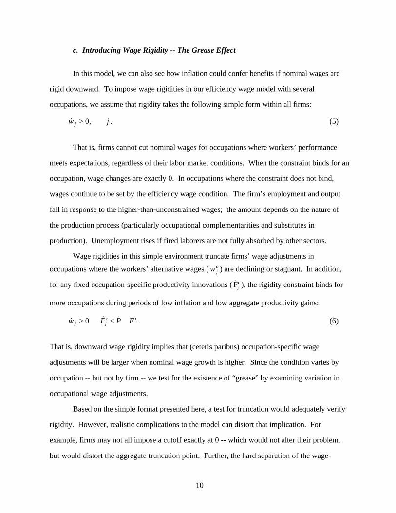
c. Introducing Wage Rigidity -- The Grease Effect

In this model, we can also see how inflation could confer benefits if nominal wages are

rigid downward. To impose wage rigidities in our efficiency wage model with several

occupations, we assume that rigidity takes the following simple form within all firms:

& ,w jj > ∀0 . (5)

That is, firms cannot cut nominal wages for occupations where workers’ performance

meets expectations, regardless of their labor market conditions. When the constraint binds for an

occupation, wage changes are exactly 0. In occupations where the constraint does not bind,

wages continue to be set by the efficiency wage condition. The firm’s employment and output

fall in response to the higher-than-unconstrained wages; the amount depends on the nature of

the production process (particularly occupational complementarities and substitutes in

production). Unemployment rises if fired laborers are not fully absorbed by other sectors.

Wage rigidities in this simple environment truncate firms’ wage adjustments in

occupations where the workers’ alternative wages ( w ja ) are declining or stagnant. In addition,

for any fixed occupation-specific productivity innovations ( ′&Fj ), the rigidity constraint binds for

more occupations during periods of low inflation and low aggregate productivity gains:

& & & &w F P Fj j> ⇒ ′ < + ′0 . (6)

That is, downward wage rigidity implies that (ceteris paribus) occupation-specific wage

adjustments will be larger when nominal wage growth is higher. Since the condition varies by

occupation -- but not by firm -- we test for the existence of “grease” by examining variation in

occupational wage adjustments.

Based on the simple format presented here, a test for truncation would adequately verify

rigidity. However, realistic complications to the model can distort that implication. For

example, firms may not all impose a cutoff exactly at 0 -- which would not alter their problem,

but would distort the aggregate truncation point. Further, the hard separation of the wage-

11

setting rule from the employment level might not hold, or other effects of inflation might move

the truncation point. For these reasons, and to maintain symmetry in our analysis, we look for

wage rigidity’s effect on the standard deviation of occupational adjustments, because truncation

always implies a reduced variance. To demonstrate the adequacy of the standard deviation,

consider wage changes truncated at c1 from the ideal ( ( )& ~ ,*w Nj µ σ ):

( )std where & & , ,*w w c M Mc

M

c

cj j > = − −−

< =

−

−

σµ

σσ

φµ

σµ

σ

1Φ

(7)

and φ and Φ are, respectively, the probability and cumulative density functions of the normal

distribution. Truncation always reduces the standard deviation of a normal distribution because

the standardized mean after truncation (M) always exceeds the standardized truncation point (the

new minimum) and is strictly positive. Since more inflation expands the distance from the mean

to a constant truncation, it will raise the standard deviation of occupational wage adjustments

when wage rigidity constraints exist.

d. Statistical Implementation of the Identification Strategy

Our analysis allows the benefits and disruptions of inflation to occur simultaneously. To

implement tests in this setting, our statistical procedure has two stages. The first decomposes

wage changes to estimate the wage adjustments that would have occurred if the effects were

independently observable, using the panel features of our dataset. The second step relates the

dispersion of two generated components to the level of inflation.

Specifically, in the first stage or our analysis, we estimate the components of occupation-

firm log wage changes, via the following fixed-effects regression:

wf j = α + ββ Df + γγ Dj + µf j, for each locality and year, (8)

where ββ and γγ are coefficient vectors for matrices of dummy variables (Df and Dj) referring to

the cell’s firm and occupation, respectively. The ββ vector measures deviations from the mean

12

wage change across the firm’s complement of occupations; i.e., the general pricing deviation

developed above (sand). The γγ vector represents average occupational wages adjustments made

in the market. Wage flexibility restrictions that occur for a collection of firms will alter the γγ

vector if relative wage adjustments occur in concert across firms. Identification relies on all

firms’ ongoing need to make occupational wage adjustments.

The second stage of the analysis links the variability of the ββ and γγ vectors of firm and

occupational coefficients to price changes through regressions of their employment-weighted

standard deviations on the level of inflation. The sand and grease hypotheses predict that the

standard deviations of the ββ and γγ vectors (respectively) will increase with the level of inflation.

Without the grease and sand complications advanced here, there is no reason to expect

any relationship between variability in these relative wage terms and inflation. That is, the

scaling effect of inflation and real wage growth has been removed by the intercept in the log

wage specification. In particular, although the quality of workers certainly varies among cells

and over time, there is no reason to expect the dispersion of worker quality among cells to have a

systematic relationship to inflation.9 Similarly, rapid shifts in demographics or technological

diffusion could alter the intensity of pressures for occupational wage adjustments, but we have

no reason to think that these changes are correlated with our measures of inflation.

However, some aspects inflation-induced wage-change variation are expected to differ

between grease and sand. This feature allows us to fashion a wide range of statistical tests of the

indentification strategy on the data analyzed here. A companion paper, Groshen and Schweitzer

(1997), reports on these probes and finds that in each case, the results are consistent with grease

and sand interpretations of our findings. For example, a priori, we also expect the standard

deviation of occupational wage changes to be bounded by the size of usual shocks to the labor

market, whereas the disruption measured by the variation in firm changes may be unbounded if

high inflation generates enough uncertainty.10

9 Reder (1955) and others have noted the impact of cyclical changes on the quality of workers employed,

but inflation is not exclusively procyclical, and changes in average worker quality do not have a predictable effecton the detailed inter-occupational or inter-firm variances considered here.

10 Expanding indexation could bound the sand effect, as suggested by Drazen and Hamermesh (1986).

13

The basic regression analysis is followed by several robustness probes to further verify

that the relationship is not spurious.

e. Labor Productivity Growth in the Model

Finally, our analysis incorporates the realization that general increases in labor

productivity can substitute for inflation in both the grease and sand stories. Since broad-based

productivity increases shift out the demand for labor, employers’ productivity-based adjustments

induce others to match them -- along with inflation -- in nominal firm-wide wage adjustments. In

light of this, we measure external wage change (CPI+) as the change in output prices plus the

general increase in labor productivity. Ceteris paribus, this sum approximates the average

nominal wage growth in the economy.

This point has policy implications to the extent that the grease and sand relationships or

their welfare costs are nonlinear. Suppose, for example, that the grease story is true, and the

beneficial impact nominal wage growth has a negative second derivative. In that case, the

beneficial grease provided by additional inflation diminish in environments with rapidly growing

productivity. Since productivity growth is indisputably beneficial beyond the factors considered

here, we focus on the role of inflation while controlling for productivity growth.

4. Description of the Data

The employer-reported wage data examined here have three major advantages compared

to those used in previous papers. Other studies examine inflation’s impact on price indices or

industry aggregates (rather than actual prices), or wage changes in household micro data. First,

the data used here are less prone to random reporting error than household data (which contain

errors in earnings and hours that can be magnified by first-differencing) because they derive from

administrative records. Second, they are longer-lived than any source previously investigated.

Third, because employer data records wages in the way most meaningful to firms, it is preferable

to household or aggregate data for studying impacts on firms’ wage-setting. This perspective

appropriately reflects the strategies used by firms to adjust wage bills (e.g., promotions,

14

reassignments or reorganization), but not the potentially confounding means used by workers

individually to adjust their earnings (e.g., taking second jobs or changing hours).

Only a few publicly-available wage data sets provide information on employers, and none

of these offers occupational detail plus a long time period.11 This study uses a data set with both

desired features, constructed from an annual private salary survey conducted in Cleveland,

Cincinnati, and Pittsburgh. The Federal Reserve Bank of Cleveland has conducted the CSS for

at least 38 years to assist its annual salary budget process. In return for their participation,

surveyed companies receive result books for their own use.

Table 2 describes the dimensions of the CSS wage-change data set. The complete CSS

data set has 80,301 job-cell-years of mean wage observations.12 From these data, we compute

67,885 annual wage changes for job cells observed in adjacent years.13 Each observation gives

the change in the log of the mean or median salary for all individuals employed in an occupation-

employer cell.14 Cash bonuses are included as part of the salary, although fringe benefits are not.

Participants in each city are chosen to be representative of large employers in the area.

The number of companies participating has grown from 66 to 96 per year (see table 3). On

average, they stay in the sample for just under 13 years each.. Since each participant judges

which establishments to include in the survey, depending on its internal organization, we use

11 See Hotchkiss (1990) for a summary of data sets with information on employers. For example,

Industry Wage Surveys and Area Wage Surveys collected by the Bureau of Labor Statistics have occupationaldetail but are not easily linked over time. Unemployment Insurance ES-202 data, when available, reportindividuals' earnings, not wages, and lack occupational detail. The Longitudinal Research Database goes back to1972, but covers only manufacturers and provides no occupational detail.

12 Unfortunately, data for some cities in some years were not found. No observations are available for1966 and 1970.

13 Job-cell-year observations where the calculated change in log wages exceeds 0.50 in absolute valueare deleted from the sample on the assumption that most of these arise from reporting or recording errors. Thiseliminates 193 observations and considerably reduces the variance of wage changes without causing anyqualitative change in the estimated coefficients reported here. Approximately 1,000 observations are imputedfrom cases where job-cells are observed two years apart. The imputed one-year changes are simply half of thetwo-year differences. Many of the results reported here were also run without the imputed observations. Theirinclusion does not affect the results.

14 Medians were recorded from 1974 through 1990. Since medians should be more robust to outliers,our results use means through 1974 and medians for the years thereafter. Comparison of the coefficientsestimated separately for means and medians for the years where both were available (1974 and 1981-1990)suggests that they are highly correlated (correlation coefficients of .97 to .99). However, coefficients estimatedwith medians show more variation than those estimated on means and are more highly correlated over time. Thelatter two characteristics are consistent with medians being a more robust measurement of central tendency.

15

"employer," a purposely vague term, to mean the employing firm, establishment, division, or

collection of local establishments for which the participating entity chooses to report wages.15

The industries included vary widely, although the emphasis is on obtaining employers with many

employees in the occupations surveyed. The employers surveyed include government agencies,

banks, manufacturers, wholesalers, retailers, utilities, universities, hospitals, and insurance firms.

The occupations surveyed (43 to 100 each year) are exclusively nonproduction jobs

which can be found in all industries, and for which markets are most developed.16 Many

occupations are divided into grade levels reflecting different degrees of responsibility and

experience. In this analysis, each occupational grade in each city is counted as a separate

occupation; thus, the total number of "occupations" in table 3 exceeds the number surveyed. On

average, each employer reports wages for 27 occupations.

Although the CSS is conducted annually, the month surveyed has changed several times

since 1955. Throughout the paper, results for any year refer to the time between the preceding

survey and the one conducted in that year (shown in Appendix A) -- usually a 12-month span,

but occasionally not. All data merged in have been adjusted (to the extent possible) to reflect

time spans consistent with those in the CSS.

Concern that the survey could be an unrepresentative sample was answered by comparing

the CSS to the Bureau of Labor Statistics’ Area Wage Surveys in the same years for the same

cities. Movements of mean wages for similar occupations were highly correlated across the two

surveys, and levels were usually within 5 percent of one another. Cleveland, Cincinnati, and

Pittsburgh are more urban, have more cyclically sensitive employment, have undergone more

industrial restructuring than the nation, and have seen their pre-1980s wage premium over the

country average gradually disappear over the last two decades.

15 Some include workers in all branches in the metropolitan area; others report wages for only the office

surveyed. Since a participant's choice of the entities to include presumably reflects those for which wage policiesare actually administered jointly, the ambiguity here is not particularly troublesome.

16 They include office (e.g., secretaries and clerks), maintenance (e.g., mechanics and painters),technical (e.g., computer operators and analysts), supervisory (e.g., payroll and guard supervisors), andprofessional (e.g., accountants, attorneys, and economists) occupations. Job descriptions for each are at least twoparagraphs long.

16

We also incorporate standard measures of inflation and national output per hour in our

analysis. As a measure of general inflation experienced in the country, we use percentage

changes in the monthly averages of the Consumer Price Index for all Urban Workers (CPI-U).17

Our labor productivity measure is the Nonfarm Business Sector Output per Hour Worked.

Table 3 shows that, despite some variations, mean log wage changes among the three

cities are highly correlated. But do they bear any relation to national wage trends? Figure 1

shows the strong correspondence between the CSS three-city mean log wage change and our

simple measure of nominal wage change (labeled CPI+) -- which equals the sum of inflation

(CPI-U) and aggregate labor productivity movements. Formalizing the observation that CSS

wage hikes are synchronized with overall price increases and productivity gains, table 4 shows

that the correlations between mean CSS wage adjustments and the CPI-U and CPI+ (0.84 and

0.74, respectively) are quite high. The anomalous negative correlation between productivity

growth and wage changes over these forty years stems from the high-inflation, low-productivity

recessions of the 1970s and early 1980s.18

To summarize, figure 1 and table 4 support the characterizations made here about the

process of wage setting during the period. They also demonstrate that wages in the CSS largely

adhere to national trends, and thus may enlighten us about the behavior of wages in the nation as

a whole. Finally, they put the remainder of the analysis into some historical perspective, lest we

forget the major influences on wages and prices that underlie our research.

5. Stage 1: The Components of Wage Adjustments

In section 3, we argue that wage adjustments have significant, distinguishable employer

and occupation components. In the present section, we verify that assertion empirically, with an

analysis of variance (ANOVA) of wage adjustments of the CSS sample (see table 5) based on

equation (8). The first two columns list sources of variation and their associated degrees of

17 Experiments with the individual city CPIs yielded very similar results. For ease of exposition, we

report only the results obtained with the national CPI.18 See Eberts and Groshen (1991) for an example of similar results.

17

freedom. Control for mean annual changes in three cities absorbs xx103 degrees of freedom. To

allow occupational wage patterns to diverge in the cities, occupation and city are interacted,

accounting for xx5,358 degrees of freedom. Employers’ mean annual wage movements absorb

another xx2,771 degrees of freedom.

The third column lists each source’s marginal contribution to the model sum of squares

(over the contributions of the sources listed above it on the table). We choose this method of

presentation -- similar to a stepwise regression -- because of its parsimony when the data are

unbalanced (i.e., the occupations in each firm varies). If joint effects are large (such as between

occupation and employer in wage levels, as shown in Groshen [1991a, 1991b]), the order of

presentation is crucial and a stepwise presentation can be misleading. Surprisingly, the joint

effects in wage-change variation between occupation and employer are minuscule; thus, the

order of presentation is not qualitatively important. Introducing occupation after employer

would alter little in this table.

All together, the model accounts for xx27.9 percent of the variation in annual wage

adjustments. That is, the R2 for the regression shown in equation (Error! Bookmark not

defined.) is xx.279. The residual variation is presumably due to compositional changes and

individual merit raises. The fifth column of the table shows that slightly more than one-fifth of

the equation’s explanatory power stems from changes common to all job cells in each year.

Intercity differences, while statistically significant, account for little of the variation. Occupation-

wide changes, on the other hand, constitute more than one-quarter of observed variation. By far

the strongest effect is employer-wide changes, which account for almost half of the explained

variation and xx13.1 percent of total variation. F-statistics for these five sources of variation are

all significant at the 1 percent level.

This decomposition suggests that the institutional model described above fits the data.

We do observe distinguishable occupation-wide and employer-wide variations in wage changes.

In particular, the firm-wide wage movements are interesting because they are such a large

component and because employer wage differentials are generally quite stable (Groshen

[1991b]), suggesting that these may be errors and corrections.

18

To the extent that employers consider their company-wide and occupational wage

adjustments separately and the relevant information for the two come from independent sources,

the standard deviations of these two wage change components will be uncorrelated over time.

Table 6 presents correlations of the annual standard deviations of the three components of wage

changes, pooling the three cities together. These correlations are all positive, suggesting that

some factors affect the variation of the components similarly. However, as the model suggests,

the intertemporal patterns of dispersion of the employer and occupation components are only

moderately correlated. The higher correlations of the standard deviations of the residual and

occupational components suggest that some adjustment of occupational differentials may not

occur uniformly across employers.19

6. Stage 2: Inflation’s Impact on Employer and Occupation Wage Changes

With this evidence that the proposed framework is reasonably consistent with the CSS

data, we turn to asking the second-stage question: how do these sources of wage adjustment

dispersion vary with inflation? All specifications use the first-stage fixed-effects coefficient

estimates summarized in table 5. In this second stage, we regress the standard deviation of the

estimated occupation and employer components -- taken from the ββ and γγ vectors estimated in

equation (8) -- on the sum of inflation and productivity increases (CPI+). To confirm the

robustness of our findings, we also perform nonparametric, filtered, and panel versions of these

tests. We close the section with a discussion of the net impact of inflation.

a. The Basic Relationship

Table 7 presents the results of the following four independent regressions of occupation

and employer wage change dispersion (stdoct and stdemt, respectively) on CPI+ (the external

proxy for annual wage movement) and CSS∆ (the equivalent internal measure):

19 Alternatively, such shifts in relative wages among occupations may stimulate simultaneous

compositional changes among job cells. That is, employers may accompany adjustments in relative wages withsome occupational reorganization of their work forces.

19

stdoc

stdem

CPI CPI

CSS CSSt

t

t t

t t

= ++ + +

+

ψ

κ κξ ξ

1 22

1 22

( ) ( )

∆ ∆ . (9)

The simple two-term quadratic expansion allows curvature in the estimates, while

remaining easily interpretable. To assist the reader with the slopes over the relevant range, we

report the implied value of the independent variable at the maximum or minimum at the bottom

of the table. Variable means appear in table 6. While the two-stage nature of this procedure may

raise standard errors in equation (9), it will not influence coefficient estimates unless the first-

stage estimation errors are correlated with our measures of inflation. We have no a priori reason

to suspect such a correlation.

Column 1 of table 7 suggests an inverted U-shape (peaking at 13.4 percent) between

employer disagreement (“sand”) and CPI+. By contrast, Column 2 suggests a U-shaped

(minimized at 2.2 percent) relationship between the dispersion of employer wage hikes and the

city-year mean. Interestingly, CSS∆ -- the internal measure of wage change -- has less

explanatory power (lower R2) than CPI+ -- the external measure. In both cases, while neither

quadratic term is independently significant, the combination of the two terms passes the F-test

for joint significance. Thus, although the exact shape is not strongly supported, the standard

deviation of employer wage hikes shows a statistically significant relationship to the level of

inflation. When plotted, these results concur that employer disagreement (our measure of the

sand story) rises substantially as mean nominal wage hikes climb from 3 to 10 percent.

However, the inconsistency between the coefficients on internal (CSS∆) and external (CPI+)

measures of wage increases and a scarcity of higher inflation data tempers our ability to say

whether the disagreement tapers off or accelerates at inflation rates above 10 percent.

Columns 3 and 4 apply the same analysis to occupational wage changes, estimating the

grease added by inflation. In this case, estimates based on the internal and external measures

agree on a statistically significant, inverted U-shaped relationship (maximized at 10 to 11

percent) between mean wage growth and occupational wage adjustments. Again, the external

measure (CPI+) has more explanatory power. Both terms in the CPI+ specification are

20

significant, providing fairly strong, consistent evidence that while inflation may grease the wheels

of occupational adjustments, any benefits are limited.

The implied relationships between CPI+ and the variability of these two components of

wage adjustment are best shown graphically. Figures 2A to 2D also confirm that the quadratic

specification fits the data remarkably well, because we plot independently-estimated, smoothed

(nonparametric) versions of the relationships alongside the parametric predictions.20 The

smoothing is similar to allowing a large number of quadratic terms, and suggests that the

parsimonious models in table 7 capture most of the curvature in these relationships. The

frequency of observations is indicated (except for overlaps) by the density of tick marks for the

smoothed estimates. Appendix figures B1-B4 present these same estimates along with scatter

plots of the underlying observations. Generally, the nonparametric approach strongly confirms

the parametric results; however, the potential importance of outliers in this specification is made

clear at the tails of figure 2D.

Over the observed range of CPI+ and CSS∆ (3 to 10 percent), each plot indicates a

positive relationship. The upward slope for employer variability appears markedly steeper than

that for occupational variability, particularly at higher rates of inflation. Also, figures 2A and 2B

show that, over the observed range of the data, the seemingly inconsistent shapes described in

columns 1 and 2 of table 7 track each other fairly well; both slope upward fairly steeply. We also

note that although the standard deviation of occupational wage changes peaks at mean wage

changes of 10 to 11 percent, the curves’ flatness suggests that little is gained beyond rates of 6 to

7 percent. Allowing for mean productivity annual growth of about 1.5 percent, these results

imply that any benefits conferred by inflation were exhausted after rates of about 5 percent.

In order to evaluate more subtle hypotheses about the shape of these relationships, we

explore their sampling variation using Efron and Tibishrani’s (1993) bootstrapping procedure

with 1000 resamplings from the first-stage estimates. Using either parametric or nonparametric

20 We choose the LOWESS smoother with a bandwidth of one, proposed by Cleveland (1979), for its

robustness with respect to both axes. Various bandwidths for 0.2 to 1 were tried, with little variation in effect.Cleveland recommends a bandwidth of 1, due to the tri-cube weighting already included in the LOWESStechnique.

21

estimates, the test confirms that occupation and employer components show distinctly different

curvatures at higher levels of inflation. At conventional significance levels, we cannot rule out

the possibility that the employer relationship slopes down at higher values of CPI+. However,

we can say with a high degree of confidence that the occupational relationship turns down before

the maximum of CPI+ (13 percent): with 93% confidence for the parametric estimates and 89%

for the nonparametric. Indeed, (with 95% confidence) the occupational relationship peaks

somewhere above 8.6% CPI+ levels for both estimation techniques. While these conclusions are

less tight than we might desire, they can be combined to describe likely ranges for the net effects

of inflation, as we do below.

Above, we report results for regressions on CPI+ without separating its two underlying

series or adding other controls (particularly the unemployment rate -- to control for cyclical

factors such as compositional changes).21 In results not reported here, when we entered the two

components of CPI+ separately, we found that most of the action in the estimated relationships

with CPI+ reflects correlations between wage change variability and inflation, not productivity

(unsurprising, since the latter is poorly measured). Nevertheless, to present our results, we favor

the parsimonious basic model (which imposes the same coefficient on changes in CPI-U and

output/hour, and omits other regressors) for five reasons: 1) As we argue above, combining

inflation and productivity is conceptually appropriate to the process under study; 2) The close

link between CSS∆ and CPI+ shown in figure 1 suggests that it is consistent with salary

administration in the CSS (the CPI-U alone is biased downward); 3) Adding the unemployment

rate to equation (9) has no qualitative effect on the coefficients of interest;22 4) This approach is

robust to concerns that the CPI-U overstates inflation and, thus, underestimates productivity

21 For the interested reader, results of some alternative specifications are available on request.22 This result rules out a compositional interpretation of our findings. Reder (1955) argues that

employers hire lower quality workers during expansions than recessions. If three conditions hold (i.e., lowerquality workers receive lower wages within cell, inflation level and unemployment rate are negatively correlated,and this effect varies by employer and occupation), our results could reflect systematic variations in workerquality. However, were this the correct interpretation of our results, then including unemployment rate--a bettermeasure of labor market conditions--should reduce the size and significance of the estimated coefficients on CPI+.The fact that unemployment rate has no impact on our estimates constitutes strong evidence against thisinterpretation.

22

growth; and, 5) This basic version simplifies our exposition and facilitates comparisons with

both the internal measure of wage growth (CSS∆) and our various robustness probes.

Under the model of wage-setting we advance, our results suggest that the disruptive sand

from additional inflation (as measured by the standard deviation of employer wage adjustments)

increases rapidly as the level rises, while the potentially beneficial grease (as measured by the

standard deviation of occupational wage adjustments) shows a slower and even diminishing

relationship with nominal wage growth. We consider net impacts at the end of this section.

b. Filtered Results

A reasonable concern with the basic specification is whether the ANOVA in the first

stage correctly identifies the underlying factors we want. While equation (8) fits neatly with the

hypotheses developed in the model, we might suspect that unmodeled terms creep into terms

collected by the fixed-effect coefficients. Though the averaging implicit in the estimation

procedure should keep these corrupting factors small, we explicitly control for them in this

section using implications of the two stories. That is, are employer wage changes largely short-

term errors and corrections, while occupational movements are market-driven adjustments?

We use the nature of the corrupting factors to filter out their effects. Specifically, the

potential corruption to the employer component is the possibility that firms alter their long-term

“market position,” a decision that is treated as infrequent in the compensation literature. This

suggests filtering out firms’ long-term adjustments to emphasize their higher-frequency errors.

Similarly, occupationally correlated errors could corrupt the occupation components.

Eliminating high-frequency changes should leave a purer measure of the presumably longer-term

adjustments of the occupational wage structure to shifts in supply or demand.

We use the filters on the first-stage regression coefficients obtained from the ANOVA

(see Appendix C). Then we calculate standard deviations for the filtered firm and occupation

components and run the same basic quadratic specifications. The results, shown in figures 3A

and 3B, generally confirm the results obtained with unfiltered components. A minor exception is

figure 3B, where the filtered, nonparametric relationship flattens earlier than either the quadratic

23

fit or the previous results. Filtering also lowers the levels of variation in the components, as

would be expected. Overall, these results are similar enough to confirm the appropriateness of

the ANOVA procedure. However, they should not be viewed as superior or replacements for

the simpler results previously presented, as the filtering process undoubtedly eliminates much of

the desired variation in the components.

c. Panel Estimates

Alternatively, the skeptic may fear that the relationships we find stem from some spurious

correlation between inflation and wage-change variability. To address these issues, we obtain

panel estimates (rather than measuring associations between aggregates), which allows us to

control for two large classes of spurious correlation. Appendix D provides further details on the

estimation technique.

The panel approach allows control for two key types of extraneous covariation:

autocorrelation in firm decisions across adjacent years, and fixed occupation or employer effects.

Despite these advantages, the panel approach is more complex expositionally and suffers from

overkill -- removing employer fixed effects almost certainly takes out nonextraneous variation

along with the extraneous. Thus, we present these results as a polar case, to show that the basic

results hold even under these stringent conditions.

Tables 8A and 8B show the results of panel regressions on CPI+ for the occupation and

employer components.23 Specification 1 in tables 8A and 8B (the panel equivalent of the

regressions in table 7) provides a basis for identifying the impact of the controls. Specifications

2, 3 and 4 add the two forms of controls separately and then together, respectively.

Not surprisingly, specification 1 obtains a very low R2 because it regresses a large cross-

section of micro observations on a single macroeconomic series. Despite the tremendous

heterogeneity of cell wage changes, the aggregate relationships we detected earlier between

CPI+ and the dispersion of employer and occupation adjustment components hold in all

23 Regressions not reported here, using the internal CSS∆ wage change measure, are comparable.

24

specifications. From a statistical view, these results strongly confirm that firm and occupation

wage change deviations rise during periods of high inflation and aggregate productivity growth.

Strikingly, even though adding controls improves the explanatory power of these

regressions, any differences in estimated coefficients on CPI+ and its square have little economic

significance. The qualitative impact of the specification changes on our occupation estimates can

be noted in the bottom two rows of table 8A, which shows that the slope of the predicted

relationship falls by less than 1 percentage point with the introduction of controls. The implied

peak shifts back, from about 7 percent to 5.2 percent. These results imply that the beneficial

impact of inflation may be exhausted at lower rates than those indicated in the basic model, but

otherwise little is affected by adding more controls.

Similarly, panel estimates in table 8B support earlier indications that the employer

variation is more strongly affected by inflation in the relevant range (implied slopes being roughly

twice those observed for interoccupational variability). Again, lags and employer fixed effects

have little qualitative impact on coefficient estimates. According to these results, the disruptive

sand caused by inflation continues to mount at least until CPI+ levels of 8 to 12 percent -- far

beyond levels where the beneficial grease is maximized -- and may not turn down at all.

In summary, the robustness of the results to these panel controls rules out a wide variety

of spurious correlations, increasing confidence in our basic results. We have tested more

explicitly whether job-cell wage-change components deviate more when the level of inflation

allows more latitude for wage adjustments, and the results are affirmative.

d. The Net Impact of Inflation

Figure 4 illustrates how previous studies that confirm inflation’s grease effect, such as

Akerlof, Dickens and Perry (1996), overstate inflation's net benefits by ignoring its costs in the

labor market. The estimates for the grease relationship, from Figure 2A, are indicated by the

lines marked with triangles (parametric and nonparametric estimates). Allowing for average

productivity growth (11/2% for the 37-year estimation period), which has already been subtracted

out in Figure 4, our results suggest that the “grease-maximizing” rate of inflation is about 71/2%.

25

Despite fundamental differences in approach, our results qualitatively agree with household data

studies which conclude that the beneficial grease effect exists and operates most immediately at

low inflation rates.24

However, netting out the previously-ignored inflation-induced disruptions to the labor

market (indicated by estimates shown with squares) yields the curve labeled “Net Effects” in

figure 4. Since grease and sand are measured in the same units and both represent deviations

from intended wage levels, they can be combined as follows (suppressing the time subscript):

( ) ( ) ( )( ) ( )( ) ( ) ( )( )

Net Benefits Prod Grease Prod = Sand Prod∆ ∆ ∆=x = x =x

stdoc CPI stdoc x stdem CPI stdem x

−

= + − − −+(10)

where stdem and stdoc are the predicted standard deviations of the employer and occupation

components (using columns 1 and 3 of table 7, respectively). Equation (10) accounts for

inflation at a some particular level of productivity growth (x), because the hypotheses developed

earlier pertain only to changes in the standard deviations, rather than to absolute levels. We

assume that gross benefits and costs of inflation are zero when the inflation rate is zero.

We graph the estimated net benefits of inflation (at an average level of productivity

growth of 1.5%) in figure 4. Including inflation's costs lower both net benefits and optimal

inflation substantially. Indeed, relative to the pure grease effect, the net effect is almost a wash.

Inflation’s benefits at the peak of the net benefit curve amount to less that 10% of the gross

benefits at the 3% inflation. Furthermore, net benefits from inflation peak at about 21/2%

inflation, so that is the highest inflation rate that could be justified on the basis of the labor

market. This peak is verified by the nonparametric estimates as well, although these estimates

offer less of a range where inflation might benefit the labor market.25

24 For example, Akerlof, Dickens and Perry conclude that the cost of setting an inflation target of 0

percent as opposed to 3 percent would raise unemployment by 1.7-2.6 percentage points.25 The nonparametric estimates are conditioned by the relative grease and sand effects of the quadratic

specification, because there is no prediction for the nonparametric estimates near CPI+=1.5%. Altering the pointswhere the conditioning occurs would shift the estimates vertically, leaving the peak unchanged but shiftinginflation rates from beneficial to derogatory or vice versa.

26

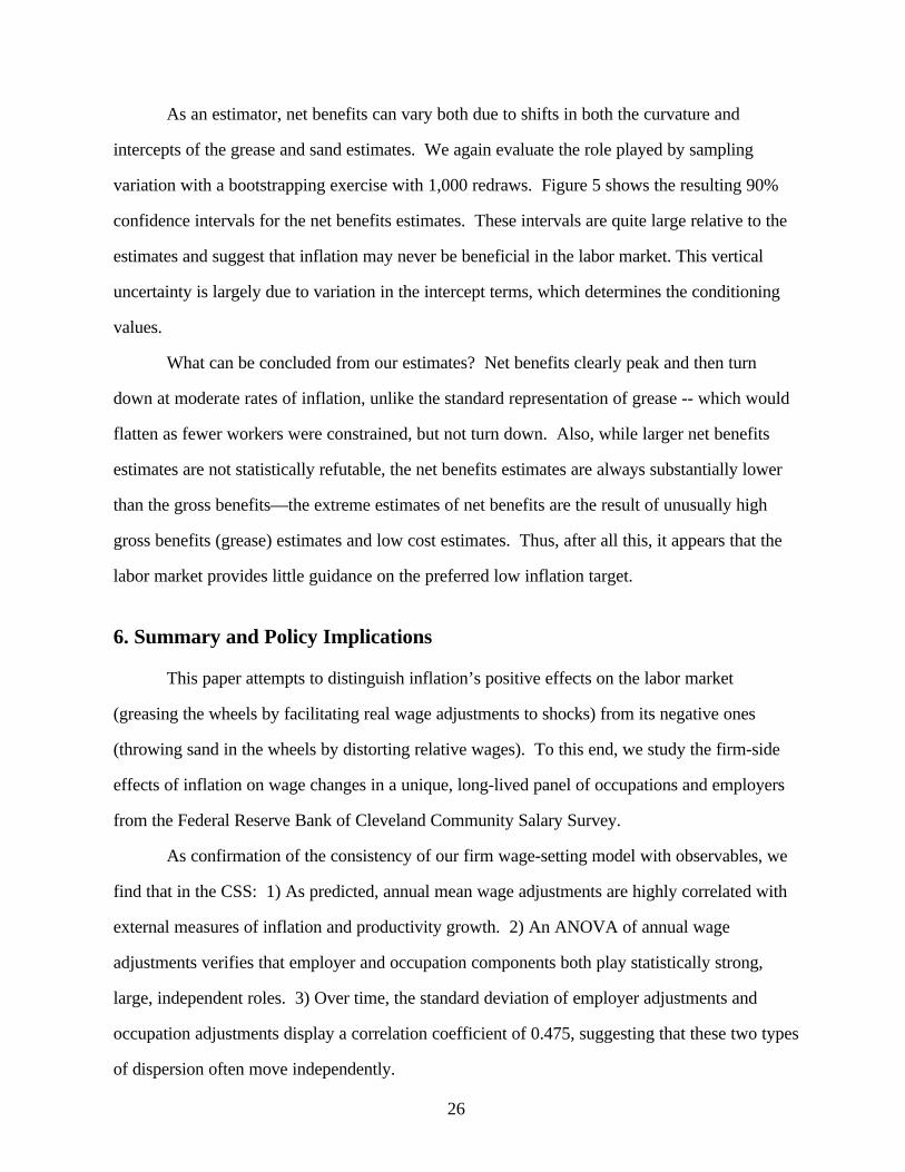
As an estimator, net benefits can vary both due to shifts in both the curvature and

intercepts of the grease and sand estimates. We again evaluate the role played by sampling

variation with a bootstrapping exercise with 1,000 redraws. Figure 5 shows the resulting 90%

confidence intervals for the net benefits estimates. These intervals are quite large relative to the

estimates and suggest that inflation may never be beneficial in the labor market. This vertical

uncertainty is largely due to variation in the intercept terms, which determines the conditioning

values.

What can be concluded from our estimates? Net benefits clearly peak and then turn

down at moderate rates of inflation, unlike the standard representation of grease -- which would

flatten as fewer workers were constrained, but not turn down. Also, while larger net benefits

estimates are not statistically refutable, the net benefits estimates are always substantially lower

than the gross benefits—the extreme estimates of net benefits are the result of unusually high

gross benefits (grease) estimates and low cost estimates. Thus, after all this, it appears that the

labor market provides little guidance on the preferred low inflation target.

6. Summary and Policy Implications

This paper attempts to distinguish inflation’s positive effects on the labor market

(greasing the wheels by facilitating real wage adjustments to shocks) from its negative ones

(throwing sand in the wheels by distorting relative wages). To this end, we study the firm-side

effects of inflation on wage changes in a unique, long-lived panel of occupations and employers

from the Federal Reserve Bank of Cleveland Community Salary Survey.

As confirmation of the consistency of our firm wage-setting model with observables, we

find that in the CSS: 1) As predicted, annual mean wage adjustments are highly correlated with

external measures of inflation and productivity growth. 2) An ANOVA of annual wage

adjustments verifies that employer and occupation components both play statistically strong,

large, independent roles. 3) Over time, the standard deviation of employer adjustments and

occupation adjustments display a correlation coefficient of 0.475, suggesting that these two types

of dispersion often move independently.

27

In our analysis of the relationship between inflation (along with labor productivity

increases) and these two kinds of wage change dispersion, we find the following:

(1) Does inflation provide grease? Yes. Consistent with recent grease studies, higherinflation and labor productivity appear to increase the range of occupational wageadjustments, although these potential benefits taper off after inflation rates of about 3-4 percent (assuming labor productivity growth of 1.5 percent, the average rate overthe period observed).

(2) Does inflation add sand? Yes. Higher inflation and labor productivity are alsoassociated with higher, potentially inefficient variation in employer wage adjustments.The variation between employer wage adjustments rises about twice as quickly asoccupational variation with respect to inflation and shows less evidence of a turndownat inflation levels over 7 percent.

The net benefits of inflation implied by these relationships are quite low and peak at moderate

rates.

We think these findings add a unique micro-level perspective to aggregate-level research

on the relationship between inflation and productivity or income growth -- studies that skip over

the mechanisms involved but presumably measure the net impact of grease plus sand on the

entire economy. For example, Rudebusch and Wilcox’s (1994) finding of a negative correlation

between the level of inflation and US productivity growth is consistent with our results that the

disruptive impact of inflation outweighs benefits obtained from greasing the wheels.26

Since we do not consider impacts of inflation beyond the labor market, our study cannot

estimate inflation’s net effect on overall productivity. However, within the labor market, our

study is the first to investigate the mechanisms involved and to measure the relevant ranges for

the grease and the sand hypotheses simultaneously.

Recent reductions in core inflation provide a strong impetus for examining how inflation

affects the labor market. How much lower should we go? Were monetary policy-makers to

adopt an inflation target, the appropriate goal would hinge on the net impact that inflation has on

26 Interestingly, if monetary authorities acted as if they were aware of the relationships identified in this

study, they might be most likely to allow moderate inflation during periods of exogenously low productivitygrowth. Such considerations would also generate a negative correlation between inflation and productivity, asobserved by Rudebusch and Wilcox (1994). Others have argued that Rudebusch and Wilcox’s results stem mostlyfrom cyclical effects.

28

the economy. Indeed, the impact of inflation in labor markets, which constitute two-thirds of

production costs, are the locus of most public concern about the effect of low inflation. Our

analysis strongly indicates that inflation is far from an unqualified benefit to the labor market and

that, at most, only rates below 2 1/2 percent could be justified on this basis.

Reinforcing our conclusion that lower inflation rates may not harm the labor market is the

additional argument that persistent low rates could relax wage rigidity -- lowering optimal

inflation further than suggested in the estimates we present here. In a low-inflation environment,

competition would pressure participants to adopt more flexible practices, such as bonus and

incentive pay, contingent contracts, etc. Intrinsically, this argument recognizes that all empirical

estimates of the benefits of inflation (including our own) assume that wage-setting practices will

not adjust. Until this country has experienced inflation rates below 3% for an extended time, or

appropriate data from some other industrial country is analyzed, we cannot be certain about the

long-run effects of low-inflation. However, our results indicate that many fears about its impact

on the labor market are probably exaggerated.

29

References

Abraham, Katharine G. and John C. Haltiwanger. “Real Wages and the Business Cycle,”Journal of Economic Literature, vol. 33, no. 3 (September 1995), pp. 1215-64.

Akerlof, George A., William T. Dickens and George L. Perry. “The Macroeconomics ofLow Inflation.” Brookings Papers on Economic Activity Q1 1996. pp. 1-74.

Allen, Steven G. “Relative Wage Variability in the United States 1860-1983,” Review ofEconomics and Statistics, vol. 69, no. 4 (November 1987), pp. 617-626.

Bewley, Truman and William Brainard. “A Depressed Labor Market, as Explained byParticipants,” Cowles Foundation, Yale University, mimeo (February 1993).

Bils, Mark J. “Real Wages over the Business Cycle,” Journal of Political Economy,vol. 93, no. 4 (1985), pp. 666-689.

Blinder, Alan S. and Don H. Choi. “A Shred of Evidence on Theories of WageStickiness,” Quarterly Journal of Economics, vol. 105 , no. 4 (November 1990),pp. 1003-1015.

Card, David. “Unexpected Inflation, Real Wages, and Employment Determination inUnion Contracts,” American Economic Review, vol. 80, no. 4 (September 1990), pp. 669-688.

Card, David and Dean Hyslop. “Does Inflation “Grease” the Wheels of the LaborMarket?” Princeton University 1996.

Cecchetti, Stephen G. “The Frequency of Price Adjustment,” Journal of Econometrics,vol. 31 (April 1986), pp. 255-274.

Cleveland, William S. “Robust Locally Weighted Regression and Smoothing ScatterPlots,” Journal of the American Statistical Association, vol. 79 (1979), pp. 829-836.

Drazen, Allan and Daniel S. Hamermesh. “Inflation and Wage Dispersion,” NationalBureau of Economic Research Working Paper no. 1811, January 1986.

Eberts, Randall and Erica L. Groshen. “Overview,” in R. Eberts and E. Groshen, eds.,Structural Changes in US Labor Markets (M.E. Sharpe: Armonk, NY, 1991), pp. 1-12.

Fischer, Stanley. “Relative Shocks, Relative Price Variability, and Inflation,” BrookingsPapers on Economic Activity, vol. 12, no. 2 (1981), pp. 381-442.

Fortin, Pierre. “The Great Canadian Slump,” Canadian Journal of Economics,forthcoming.

30

Freedman, Audrey. The New Look in Wage Policy and Employee Relations, TheConference Board, Report No. 865, 1976.

Friedman, Milton. “Nobel Lecture: Inflation and Unemployment,” Journal of PoliticalEconomy, vol. 85, no. 3 (1977), pp. 451-472.

Groshen, Erica L. “Sources of Intra-Industry Wage Dispersion: How Much DoEmployers Matter?” Quarterly Journal of Economics, vol. 106, no. 3 (1991a), pp. 869-84.

Groshen, Erica L. “Do Wage Differences among Employers Last?” Federal Reserve Bankof Cleveland, Working Paper 8906, June 1989 (revised 1991b).

Groshen, Erica L. “Five Reasons Why Wages Vary Among Employers,” IndustrialRelations, vol. 30, no. 3 (Fall 1991c), pp. 350-81.

Groshen, Erica L. and Mark Schweitzer. “Identifying Inflation’s Grease and Sand Effectsin the Labor Market,” in Martin Feldstein, ed., The Costs and Benefits of Achieving PriceStability, University of Chicago Press 1998, forthcoming.

Haley, James. “Theoretical Foundations for Sticky Wages,” Journal of EconomicSurveys, vol. 4, no. 2 (1990), pp. 115-155.

Hamermesh, Daniel S. “Inflation and Labour-Market Adjustment,” Economica, vol. 53(February 1986), pp. 63-73.

Holzer, Harry J. and Edward B. Montgomery. “Asymmetries and Rigidities in WageAdjustments by Firms,” National Bureau of Economic Research Working Paper No. 3274,March 1990.

Hotchkiss, Julie L. “Compensation Policy and Firm Performance: An AnnotatedBibliography of Machine-Readable Data Files,” Industrial and Labor Relations Review, vol. 43,no. 3 (February 1990), pp. S274-289.

Kaufman, Roger T. “On Wage Stickiness in Britain’s Competitive Sector,” BritishJournal of Industrial Relations, vol. 22, no. 1 (1984), pp. 101-112.

Lach, Saul, and Daniel Tsiddon. “The Behavior of Prices and Inflation: An EmpiricalAnalysis of Disaggregated Price Data,” Journal of Political Economy, vol. 100, no. 2 (1992),pp. 349-389.

Lebow, David E., David J. Stockton, and William L. Wascher. “Inflation, Nominal WageRigidity, and the Efficiency of Markets,” Division of Research and Statistics, Board ofGovernors of the Federal Reserve System, mimeo, August 1993.

Levine, David I. “Fairness, Markets, and Ability to Pay: Evidence from CompensationExecutives.” American Economic Review, vol. 83, no. 5 (December 1993), pp. 1241-1259.

31

McLaughlin, Kenneth J. “Rigid Wages?” Journal of Monetary Economics Get NewCite!

Reder, Melvin. “The Theory of Occupational Wage Differentials.” American EconomicReview, vol. 45, no. 5 (December 1955), pp. 833-852.

Reinsdorf, Marshall. “New Evidence on the Relation between Inflation and PriceDispersion,” American Economic Review, vol. 84, no. 3 (June 1994), pp. 720-731.

Rudebusch, Glenn D. and David Wilcox. “Productivity and Inflation: Evidence andInterpretations,” Federal Reserve Board, Washington, D.C., unpublished paper (May 1994).

Sheshinski, Eytan and Yoram Weiss. “Inflation and Costs of Price Adjustment,” Reviewof Economic Studies, vol. 44, no. 2 (June 1977), pp. 287-303.

Slichter, Sumner and Heinz Luedicke. “Creeping Inflation -- Cause or Cure?” Journal ofCommerce, 1957, pp. 1-32.

Stigler, George J. and James K. Kindahl. The Behavior of Industrial Prices, NationalBureau of Economic Research General Series No. 90 (New York: Columbia University Press,1970).

Tobin, James. “Inflation and Unemployment,” American Economic Review, vol. 62, no. 1(March 1972), pp. 1-18.

Vining, Daniel R. and Thomas C. Elwertowski. “The Relationship between RelativePrices and the General Price Level,” American Economic Review, vol. 66, no. 4 (September1976), pp. 699-708.

Appendix C: Applying a LOWESS Smoother for Filtering Data

The goal of our filtering procedure is to isolate long-run and short-run movements in the

occupation and employer terms derived from the stage one estimates. We want our long-run

movements to reflect the possibility of multi-year cycles or trends. A quadratic smoother (which

merely fits a quadratic of n terms to the data) would have satisfied this requirement, but is

sensitive to the existence of larger outliers in the trend. LOWESS smoother were proposed by

Cleveland (1979) to fit trends in data where outliers might be a problem.

LOWESS estimates the slope of the smooth curve in the vicinity of each observation (xi)

by employing a weighed regression on all observations within the desired range or bandwidth

[x-,x+]. The LOWESS weights limits the role of distant observations, even within the bandwidth

of the smoother:

[ ]wx x

x x x xx x xj

j i

i ij= −

−

− −

∈+ −

− +1

3 3

max( , ), , .

For our purposes, we found that a bandwidth of one (include all data) yielded a sensible

split of long-run and short-run adjustments in the employer and occupation terms. Narrower

bandwidths place more variation in the long-run portion, but our results did not appear overly

sensitive to alternative bandwidths.

Appendix D. Panel Estimation Technique

In contrast to the basic model, the panel estimates associate inflation with the absolute

deviations (rather than standard deviations) of occupation and employer components of wage

adjustments. For the occupation regressions, we take the absolute value of the fixed-effects

coefficients from equation (3), and weight them by the number of cells they represent. Employer

absolute deviations are constructed similarly. We then regress the absolute deviations of the cells

-- separately for occupation and employers -- on CPI+ and two kinds of controls, as follows:

abdoc

abdem

abdoc

abdemCPI CPI

j t

f t

j

f

j t

f tt t=

+

+ +−

−

δδ

θ ϕ ϕ,

,( ) ( )

1

11 2

2+ + , (10)

where abdocj t and abdemf t represent the absolute value of occupation and firm components for a

job cell, the δ’s are firm or occupation fixed effects, and t-1 indicates the lagged dependent

variables. The brackets indicate terms that are included in only some of the regressions.

Conveniently, the regression predictions are conditional mean absolute deviations, which are

comparable, though not identical, to standard deviations.

The panel approach allows introduction of firm fixed effects and lagged terms. Including

fixed effects controls for some firms’ or occupations’ long-run propensity to deviate more or less

than others and also for sample drift in the survey over time (that might somehow be correlated

with inflation). The lags control for the previous period’s adjustment in an occupation or firm:

for example, the case of firms that adjust wages in alternate years -- oscillating between large

positive and negative adjustments relative to firms that adjust their wages more often. While

more complicated panel specifications could be tried, the fixed effect and lagged specification

should eliminate large classes of potential spurious effects by verifying the continued relationship

despite the addition of these controls.

Table 1

Factors Influencing Wage and Salary Budgets

Nonexecutive, Exempt Nonunion, HourlyManufacturing Manufacturing

Consumer Industrial Banks Consumer Industrial BanksArea surveys 48% 41% 57% 46% 40% 39%Cost-of-living index 39 30 24 26 25 18Corp. financial results 31 50 45 21 19 30Corp. financial prospects 30 37 41 16 18 30Internal equity among

employee groups27 27 15 24 10 8

Worker productivity 15 16 34 9 5 20Increases given by

industry leaders30 35 13 23 11 3

Ability to hire 15 19 11 8 11 6Nationally bargained

settlements6 5 1 20 17 3

Union demands 10 4 − 15 17 −

Note: Multiple answers were allowed, so percentages do not sum to 100.Source: Freedman (1976).

Table 2

Description of the Annual Wage Adjustment Data SetDrawn from the CSS, 1956-1992

Total Number of Job-Cell Wage Adjustments Observed 67,885

Number of Years 36

Average Number of Observations Per Year 1,886

Mean Log Wage Adjustment 0.050

Standard Deviation of Log Wage Adjustment 0.083

Number of Occupations Ever Observed 166

Number of Occupation*City*Year Observations 5,271

Avg. No. of Occupation*City Observations Per Year 146

Number of Employers Ever Observed 192

Number of Employer-years 2716

Average Number of Employers Per Year 75

Note: All numbers reported are for the first-differenced data set.Source: Authors' calculations from the Federal Reserve Bank of ClevelandCommunity Salary Survey.

Table 3

Description of Data by Year

Number of: Mean Log Wage Adjustment in:End Year Job cells Occupations Employers Cleveland Cincinnati Pittsburgh

1957 1,336 94 73 0.051 0.046 0.0451958 1,557 94 83 0.049 0.054 0.0501959 1,714 103 88 0.040 0.048 0.0701960 1,669 103 86 0.036 0.032 0.0341961 1,701 103 88 0.039 0.035 0.0361962 1,881 109 93 0.024 0.022 0.0241963 1,910 112 90 0.019 0.026 0.0241964 2,032 113 96 0.026 0.022 0.0231965 2,123 124 95 0.021 0.026 0.0101966 1,965 125 89 0.040 0.045 0.0381967 1,967 125 89 0.037 0.042 0.0351968 2,128 124 94 0.046 0.044 0.0421969 1,972 114 97 0.066 0.050 0.0491970 853 49 36 0.068 * *1971 854 49 36 0.061 * *1972 1,262 66 38 0.061 * *1973 1,477 90 57 0.056 0.095 *1974 1,335 96 73 0.126 0.084 0.1391975 1,379 101 73 0.074 0.063 0.0901976 1,391 104 72 0.065 0.057 0.0781977 789 60 72 0.030 0.021 0.0521978 1,674 197 68 0.052 0.063 0.0661979 2,418 267 75 0.064 0.071 0.0691980 2,689 295 79 0.095 0.074 0.0871981 2,196 186 83 0.086 0.089 0.0591982 2,185 193 82 0.072 0.092 0.0781983 2,013 190 75 0.050 0.055 0.0731984 2,274 213 80 0.047 0.058 0.0631985 2,272 212 79 0.040 0.044 0.0421986 2,396 220 82 0.042 0.044 0.0371987 2,437 226 80 0.031 0.037 0.0381988 2,401 222 82 0.036 0.037 0.0231989 2,407 225 81 0.045 0.041 0.0361990 2,505 222 84 0.052 0.046 0.0241991 2,536 223 89 0.038 0.045 0.0351992 2,187 222 80 0.039 0.045 0.043Total 68,839 5,462 2,875 0.050 0.052 0.048

* In 1970-72, the CSS is missing Cincinnati; in 1970-73, the CSS is missing Pittsburgh.Source: Authors' calculations from the Federal Reserve Bank of Cleveland Community Salary Survey.

Table 4

Correlation Coefficients between CSS Wage Adjustmentsand Relevant Economic Indicators

CSS Mean Current CPI+ LaborLog WageAdjustment

CPI-U Productivity

Current CPI-U* 0.839(0.000)

CPI+* (CPI-U + Prod.) 0.737 0.861(0.000) (0.000)

Labor Productivity* -0.482 -0.601 -0.112(0.003) (0.000) (0.510)

Mean 0.051 0.046 0.062 0.015(Standard Deviation) (0.022) (0.035) (0.028) (0.018)

*Percent change experienced during the period.Note: Numbers in parentheses below the reported correlation coefficients are the probabilitythat the correlation coefficient equals 0. Total number of observations: 37.Source: Authors' calculations from the Federal Reserve Bank of Cleveland Community SalarySurvey.

Table 5

ANOVA of Annual Wage Adjustments in the CSS, 1957-1992

Source ofVariation

Degreesof

Freedom

MarginalContribution

to Sum ofSquares

Percentof TotalSum ofSquares

Percentof ModelSum ofSquares

StepwiseF-Statistic

City 2 0.1 0.0 0.1 10.3Year 35 27.7 6.0 21.5 123.5Year*City 63 3.2 0.7 2.5 8.0Occ*Year*City 5,270 37.5 8.1 29.1 1.2Employer*Year 2,716 60.4 13.1 46.9 4.5

Model 8,086 128.8 27.9 100.0Residual 59,798 333.3 72.1 .

Total 67,884 462.1 100.0

*The three cities are Cleveland, Cincinnati, and Pittsburgh. The years are 1956-1957 through1991-1992. Overall, 166 occupations are ever surveyed; in the ANOVA, each occupation iscounted separately for each city in each year. Similarly, a total of 192 employers are everobserved.Source: Authors' calculations from the Federal Reserve Bank of Cleveland Community SalarySurvey.

Table 6

Standard Deviations and Correlationsof Components of Annual Wage Changes

Component:Total Occupation Employer Residual

Mean StandardDeviation of WageAdjustments

0.0775 0.0273 0.0333 0.0670

(Std. Dev.) (0.0191) (0.0108) (0.0130) (0.0164)

Correlation ofStandard Deviationwith:Occupation Std. Dev. 0.766Employer Std. Dev. 0.676 0.475Residual Std. Dev. 0.965 0.719 0.479

Note: All correlations are significant at the 0.0001 level. Total number of city-year observations: 104.Source: Authors' calculations from the Federal Reserve Bank of Cleveland Community Salary Survey.

Table 7

Wage Inflation and the Standard Deviationof Employer and Occupation Nominal Wage Adjustments

Dependent VariableStandard Deviation of Wage Adjustment

Components:Employer Occupation

Model 1 2 3 4

Intercept 0.012 0.029 0.004 0.012(0.007) (0.006) (0.005) (0.004)

CPI+* 0.394 0.458(0.198) (0.136)

Squared CPI+* -1.475 -2.293(1.227) (0.843)

CSS Mean -0.089 0.281Adjustment (CSS∆) (0.176) (0.122)

Squared CSS Mean 2.008 -1.267Adjustment (CSS∆2) (1.328) (0.917)

Adjusted R-Squared 0.138 0.107 0.151 0.111No. of Observations 101 101 101 101F Stat. for joint test,1% cutoff ≈ 4.82

8.97 7.01 9.86 7.22

Implied ExtremaCPI+* Max:

13.4%Max:10.0%

CSS MeanAdjustment (CSS∆)

Min:2.2%

Max: 11.1%

*CPI+ is the sum of the annual change in the BLS Consumer Price Index for all UrbanWorkers (CPI-U) and the BLS Nonfarm Business Sector Output per Hour Worked.Note: Numbers in parentheses are standard errors.Source: Authors' calculations from the Federal Reserve Bank of Cleveland CommunitySalary Survey.

Table 8A

Wage Inflation and the Standard Deviationof Occupation Nominal Wage Adjustments

Dependent VariableAbsolute Value of the Occupational Wage

Adjustment Term:Model 1 2 3 4

Intercept 0.006 0.006 0.009 0.011(0.0004) (0.0004) (0.0004) (0.0004)

Lagged 0.222 0.002Adjustment (0.0037) (0.0038)

CPI+* 0.245 0.142 0.182 0.117(0.0120) (0.0119) (0.0107) (0.0119)

Squared CPI+* -1.104 -0.578 -0.797 -0.410(0.0749) (0.0745) (0.0662) (0.0680)

Fixed Effects Included None None Occupationx City

Occupationx City

Adjusted R-Squared 0.0158 0.066 0.254 0.250No. of Observations 67,885 62,871 67,885 62,871Implied Slope withrespect to CPI+*

Mean ± one STD 5.45% 4.29% 4.45% 4.62%Min. and max. of data 6.99% 5.10% 5.57% 5.20%

*CPI+ is the sum of the annual change in the BLS Consumer Price Index for all UrbanWorkers (CPI-U) and the BLS Nonfarm Business Sector Output per Hour Worked.Note: Numbers in parentheses are standard errors.Source: Authors' calculations from the Federal Reserve Bank of Cleveland CommunitySalary Survey.

Table 8B

Wage Inflation and the Standard Deviationof Employer Nominal Wage Adjustments

Dependent VariableAbsolute Value of the Employer Wage Adjustment

Term:Model 1 2 3 4

Intercept 0.013 0.012 0.013 0.012(0.0006) (0.0005) (0.0005) (0.0005)

Lagged 0.180 0.115Adjustment (0.0036) (0.0036)

CPI+* 0.148 0.086 0.159 0.116(0.0158) (0.0156) (0.0153) (0.0152)

Squared CPI+* -0.225 -0.028 -0.238 -0.134(0.0986) (0.098) (0.0946) (0.0953)

Fixed Effects Included None None Employer xCity

Employer xCity

Adjusted R-Squared 0.0185 0.054 0.120 0.133No. of Observations 67,885 62,553 67,885 62,553Implied Slope withrespect to CPI+*

Mean ± one STD 10.94% 8.07% 11.85% 9.33%Min. and max. of data 11.26% 8.11% 12.18% 9.52%

*CPI+ is the sum of the annual change in the BLS Consumer Price Index for all UrbanWorkers (CPI-U) and the BLS Nonfarm Business Sector Output per Hour Worked.Note: Numbers in parentheses are standard errors.Source: Authors' calculations from the Federal Reserve Bank of Cleveland CommunitySalary Survey.

Appendix

Salary Survey Year Salary Survey Coverage1956 March 1955 - March 19561957 March 1956 - March 19571958 March 1957 - March 19581959 March 1958 - March 19591960 March 1959 - March 19601961 March 1960 -March 19611962 March 1961 - March 19621963 March 1962 - March 19631964 March 1963 - March 19641965 March 1964 - March 19651966 March 1965 - March 19661967 March 1966 -March 19671968 March 1967 - March 19681969 March 1968 - March 19691970 March 1969 - March 19701971 March 1970 - March 19711972 March 1971 - March 19721973 March 1972 - March 19731974 March 1973 - September 19741975 September 1974 - September 19751976 September 1975 - September 19761977 September 1976 - September 19771978 September 1977 - September 19781979 September 1978 - July 19791980 July 1979 - August 19801981 August 1980 - June 19811982 June 1981 - June 19821983 June 1982 - June 19831984 June 1983 - April 19841985 April 1984 - April 19851986 April 1985 - April 19861987 April 1986 - April 19871988 April 1987 - April 19881989 April 1988 - July 19891990 July 1989 - July 19901991 July 1990 - July 19911992 July 1991 - July 1992

Figure 1: CSS Mean Wage Change Versus CPI+,+, 1957-1996

0

0.02

0.04

0.06

0.08

0.1

0.12

0.14

57 59 61 63 65 67 69 71 73 75 77 79 81 83 85 87 89 91 93 95

Year

Percent

Css Mean Wage Change CPI+

Figure 2A: Density of CSS Employer Adjustments During High and LowInflation Years

Log Wage Change Deviations

Figure 2B: Density of CSS Occupational Adjustments During High and LowInflation Years

Log Wage Change Deviations

Figure 3A: Standard Deviations of CSS Employer Adjustments Associatedwith CPI+ on Extended Sample: Nonparametric and RegressionPredictions

Inflation + Productivity Growth (CPI+)

Figure 3B: Standard Deviations of CSS Occupational AdjustmentsAssociated with CPI+ on Extended Sample: Nonparametric andRegression Predictions

Inflation + Productivity Growth (CPI+)

Note: In each case, the smooth line is the fitted quadratic relationship, while thekinked line is the nonparametric version of the same relationship.

Figure 4: Aggregate Relationship Between US Unemployment Rate and CPI+ (CPI-U Plus Change inOutput/Hour), 1956 - 1996

0

2

4

6

8

10

12

0 2 4 6 8 10 12 14

Inflation + Productivity Growth (CPI+)

Un

emp

loym

ent

Rat

e

Unemployment Rate

Regression Fit

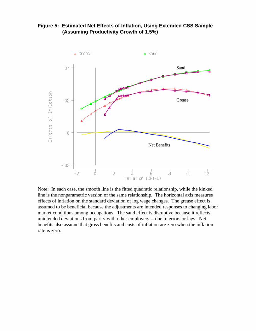
Figure 5: Estimated Net Effects of Inflation, Using Extended CSS Sample(Assuming Productivity Growth of 1.5%)

Net Benefits

Grease

Sand

Note: In each case, the smooth line is the fitted quadratic relationship, while the kinkedline is the nonparametric version of the same relationship. The horizontal axis measureseffects of inflation on the standard deviation of log wage changes. The grease effect isassumed to be beneficial because the adjustments are intended responses to changing labormarket conditions among occupations. The sand effect is disruptive because it reflectsunintended deviations from parity with other employers -- due to errors or lags. Netbenefits also assume that gross benefits and costs of inflation are zero when the inflationrate is zero.

Figure 6: Simulated Net Effects of CPI+ (CPI-U Plus Change in Output/Hour) on Unemployment, Based on CSS Results

0.00%

0.20%

0.40%

0.60%

0.80%

1.00%

1.20%

1.40%

0 2 4 6 8 10 12

Un

emp

loym

ent

Rat

e

(0.3, -0.3)

(0.0, -0.3)

(0.6, -0.2)

(0.1, -0.1)

(0.3, -0.5)

Assumed Elasticities

(Labor Supply, Labor Demand)

Inflation + Productivity Growth (CPI+)