The Effects of Geographic Expansion on Bank Efficiency

Allen N. Berger Board of Governors of the Federal Reserve System

Washington, DC 20551 U.S.A. and

Wharton Financial Institutions Center Philadelphia, PA 19104 U.S.A.

Robert DeYoung Federal Reserve Bank of Chicago

Chicago, IL 60604 U.S.A.

Forthcoming in: Journal of Financial Services Research

The opinions expressed do not necessarily reflect those of the Federal Reserve Board, the Chicago Reserve Bank, or their staffs. The authors thank the anonymous referee, Tim Hannan, Joe Hughes, Iftekhar Hasan, Dave Humphrey, Moshe Kim, Knox Lovell, Ana Lozano-Vivas, Loretta Mester, Andrew Meyer, Jesus Pastor, Subhash Ray, Tony Saunders, Steve Seelig, Phil Strahan, Larry Wall, Larry White, and other participants at the Miguel Hernández University Banking and Finance Workshop, Western Economic Association meetings, Financial Management Association Meetings, and the Federal Reserve Committee on Financial Structure and Regulation for helpful comments, and Kelly Bryant and Nate Miller for outstanding research assistance. Please address correspondence to Allen N. Berger, Mail Stop 153, Federal Reserve Board, 20th and C Streets. NW, Washington, DC 20551, call 202-452-2903, fax 202-452-5295, or email aberger@frb.gov, or to Robert DeYoung, Economic Research Department, Federal Reserve Bank of Chicago, 230 South LaSalle Street, Chicago, IL 60604, 312-322-5396 (voice), 312-322-2357 (fax), robert.deyoung@chi.frb.org.

The Effects of Geographic Expansion on Bank Efficiency

Abstract

We assess the effects of geographic expansion on bank efficiency using cost and profit efficiency for over

7,000 U.S. banks, 1993-1998. We find that parent organizations exercise some control over the efficiency of

their affiliates, although this control tends to dissipate with distance to the affiliate. However, on average,

distance-related efficiency effects tend to be modest, suggesting that some efficient organizations can overcome

any effects of distance. The results imply there may be no particular optimal geographic scope for banking

organizations � some may operate efficiently within a single region, while others may operate efficiently on a

nationwide or international basis.

JEL classification codes: G21, G28, G34, G38 Key words: Banks, Efficiency, Mergers, Financial institutions.

1

The banking industry is consolidating around the globe in response to regulatory changes and other

factors. The U.S. banking structure has not yet fully adapted to the Riegle-Neal Act, which permits bank

branching on almost a nationwide basis, and the Gramm-Leach-Bliley Act, which permits relatively

unrestricted universal banking powers for well-capitalized financial holding companies. In the European

Union, the financial structure has not yet fully adapted to the Single Market Programme, which essentially

allows continent-wide universal banking with a single license, and monetary union, which provides for a single

currency for most of the continent. In Asia, consolidation is occurring in reaction to recent banking and

financial crises. These changing factors, along with the globalization of financial markets in general, have also

created opportunities for intercontinental financial organization mergers and acquisitions (M&As). In most

cases, the consolidation activity involves geographic expansion � financial organizations expanding to other

locations within their home regions; into other regions within their home nation; or into other host nations, any

of which may be considerable distances away.

The purpose of this paper is to assess the effects of this geographic expansion on bank efficiency. On

the one hand, geographic expansion may allow efficiently managed institutions to �export� their superior

managerial skills and policies and procedures to distant affiliates; take advantage of network economies; and

exploit the benefits of geographic risk diversification. On the other hand, operating a far-flung banking empire

may reduce efficiency as senior managers stray into markets in which they have less core competence; as

organizational diseconomies arise (such as agency problems in monitoring junior managers in a distant locale);

and as distance makes providing relationship-based services to local customers more difficult. We investigate

these effects of geographic expansion on efficiency by addressing three related questions:

1) Can parent financial organizations control the efficiency of their affiliates by exporting their skills/policies/procedures, and does this control vary with distance to the affiliate?

2) Does the efficiency of an affiliate vary with its distance from its parent organization? 3) Are some individual financial organizations able to exercise more control and function

more efficiently as geographically dispersed organizations than others? It is important to distinguish between the concept of control and the level of efficiency. More control implies

that the efficiency of affiliate banks will be more similar to the efficiency of the parent. That is, the controlling

organization can export either high or low quality managerial skills/policies/procedures.

2

We address these questions by conducting three distinct empirical analyses -- a bivariate analysis, a

regression analysis, and an individual organization analysis. Each of these analyses uses estimates of cost and

profit efficiency for over 7,000 U.S. banks from 1993 to 1998. The data provide an excellent laboratory for

analyzing the efficiency effects of geographic expansion because the U.S. is a geographically large nation with

long distances between banks in the same bank holding company (BHC). Over this time period, banks were

generally allowed to operate in only one state (although their parent BHCs could own banks in multiple states),

so the location of the bank is a fairly good indicator of where it operated and achieved its efficiency scores.

These data allow us to observe how well organizations control the efficiency of distant affiliates and whether

affiliate efficiency varies with distance from the parent. Importantly, our observations are not confounded by

differences in language, culture, currency, regulatory/supervisory structures, etc. that may plague studies of

banks operating across international borders.

Our bivariate analysis compares the efficiency of banks located in the same geographic region as their

parent organization, the efficiency of banks located in geographic regions contiguous to their parents, and the

efficiency of banks located in regions that are not contiguous to their parents. We also compare the efficiency

of home-region banks whose parent organizations own banks only in that same region, home-region banks

whose parents own banks in contiguous regions, and home-region banks whose parents own banks in

noncontiguous regions. Thus, we are able to see how geographic expansion into nearby and far away locations

affects the efficiency of both distant affiliates and home-region banks. This analysis primarily addresses

question (2) above about the relationship between distance and the level of efficiency.

Our regression analysis focuses on what determines the efficiency of affiliates in multibank holding

companies. We regress affiliate bank efficiency on the efficiency of the lead bank in the BHC, the distance

between the affiliate and the lead bank, and other variables. Our maintained assumption is that the senior

management of the organization is located at the lead bank and that the performance of the lead bank is

representative of the organization�s skills, policies, and procedures. We use the coefficient on lead bank

efficiency as an indicator of parental control; we use the coefficient on distance as an indicator of the effect of

distance on affiliate efficiency; and we use the coefficient on the interaction of lead bank efficiency and

distance to indicate the degree to which parental control varies with distance. This analysis addresses both

3

questions (1) and (2) above about the effects of organizational control and distance on efficiency. We also

estimate subsample regressions for affiliates located in different states than, in different regions from, and in

regions noncontiguous to, their parents. By testing whether organizations that choose greater geographic scope

tend to be those that are relatively good at exercising control at a distance, these regressions address question

(3) above about whether some individual organizations are better at control and efficiency than others.

Our individual organization analysis focuses on the efficiency of individual banking organizations, as

opposed to the bivariate and regression analyses, which focus on the efficiency of the average bank affiliate.

We start by identifying all BHCs with 10 or more affiliates in our data. From that group, we identify �efficient

BHCs� whose affiliates tend to operate with above-average efficiency regardless of where they are located � in

the BHC�s home state, in the BHC�s home region, or in regions contiguous or noncontiguous to the BHC�s

home region. Finally, we check to see whether any one particular geographic strategy � such as statewide,

regional, or superregional banking � is predominant among these efficient BHCs. This analysis primarily

addresses question (3) above about whether some individual institutions are better at control and efficiency

than others.

Of the three analyses, we put the greatest emphasis on the regression analysis because it is the most

direct and comprehensive approach to addressing the three questions above. The bivariate and individual

organization analyses shed additional light on questions (2) and (3), respectively, and corroborate the findings

of the regression analysis.

The paper unfolds as follows. Section 1 reviews some previous research that has touched on the issues

of control and distance. Section 2 discusses the efficiency advantages and disadvantages of geographic

expansion. Section 3 explains how we measure bank efficiency and describes our data. Sections 4, 5, and 6

present the results of our bivariate, regression, and individual organization analyses, respectively, and explain

how these results answer the three main research questions asked above. Section 7 provides brief concluding

remarks.

1. Review of related research literature

To our knowledge, no prior research has directly addressed our three main questions about the effects

of organizational control and distance on bank efficiency. Specifically, we know of no prior studies that have

4

investigated affiliate efficiency as a function of the efficiency of the parent organization to assess the degree of

organizational control; none that have measured distances between affiliates and parent organizations to assess

the effect of distance on efficiency; and none that have examined the patterns of affiliate efficiency within

individual banking organizations to see if some organizations are able exercise more control and function more

efficiently as geographically dispersed organizations than others.

However, some prior research has come close to these issues. With respect to the control issue, there is

some research on the effects of BHC affiliation on the efficiency of the organization as a whole. While

efficiency of the organization is not the same concept as control, it would be expected that organizations in

which senior management is able to exercise more control would also be more efficient, all else equal. The

empirical results are mixed. For example, some studies found that banks in BHCs are more efficient than

independent banks (e.g., Spong, Sullivan, and DeYoung 1995, Mester 1996). In contrast, other research

suggested that branch banking organizations are more efficient than multibank BHCs (e.g., Grabowski,

Rangan, and Rezvanian 1993), and that for a given organization size, a greater number of separate bank

charters reduces the market value of the organization (Klein and Saidenberg 2000).

Some inference on the control issue may also be gleaned from the research on the efficiency of bank

branches. If senior management is able to effectively control the operations of individual branches, then the

efficiencies of the individual branches would be expected to be clustered near the performance of the best

practice branch of the bank. If senior management is not in control, then the efficiencies of the individual

branches would be expected to be widely dispersed. Studies of the branching networks of large U.S. banks

(e.g., Sherman and Ladino 1995, Berger, Leusner, and Mingo 1997) and of a large Canadian bank (Schaffnit,

Rosen, and Paradi 1997) found efficiencies almost as dispersed as those typically found in studies of unrelated

banks, consistent with relatively weak control for the senior management of the bank. In contrast, a number of

nonparametric efficiency studies that mostly used small numbers of branches (usually for European banks)

typically found relatively tight distributions of branch efficiency, with mean efficiency exceeding .90 (e.g.,

Sherman and Gold 1985, Zenios, Zenios, Agathocleous, and Soteriou 1996, Parkan 1987, Oral and Yolalan

1990, Vassiglou and Giokas 1990, Giokas 1991, Al-Faraj, Alidi, and Bu-Bshait 1993, Pastor 1993, Tulkens

1993, Tulkens and Malnero 1994, Drake and Howcroft 1995, Athanassopoulos 1997, 1998). This last finding

5

could reflect very tight managerial control over branch operations or it could alternatively reflect a problem

with nonparametric methods that arises when the number of observations is relatively small.

Some research has examined the effects of geographic expansion within a nation of banking

organizations as a whole and found generally favorable effects. Some found that larger, more geographically

integrated institutions tend to have better risk-expected return frontiers (e.g., Hughes, Lang, Mester, and Moon

1996, 1999, Demsetz and Strahan 1997). Others found that banking organization M&As raise profit efficiency

in a way consistent with the benefits of improved geographic diversification, but does not have much effect on

cost efficiency (e.g., Berger and Humphrey 1992, Akhavein, Berger, and Humphrey 1997, Berger 1998).

These studies generally found that the difference in efficiency between the acquirer and target had relatively

little effect on overall efficiency improvement following consolidation, suggesting that the ability of acquirers

to export superior skills/policies/procedures to targets may be limited. However, these studies did not examine

the efficiency of the individual affiliates of the organizations, did not directly address the issue of intra-

organizational control, and did not measure the distance from the parent organization.

Other research has examined efficiency across international borders, which is usually associated with

significant geographic expansion. Most studies found that foreign affiliates in a host nation are less efficient

on average than the domestic banks in that nation (e.g., DeYoung and Nolle 1996, Hasan and Hunter 1996,

Mahajan, Rangan, and Zardkoohi 1996, Chang, Hasan, and Hunter 1998, Miller and Parkhe 1999, Parkhe and

Miller 1999, Berger, DeYoung, Genay, and Udell 2000), while some found that foreign institutions have about

the same average efficiency as domestic institutions (e.g., Vander Vennet 1996, Bhattacharya, Lovell, and

Sahay 1997, Hasan and Lozano-Vivas 1998). These findings would appear to conflict with the within-nation

results cited above, in which geographic expansion appeared to be favorable on balance. However, as noted

above, cross-border expansion is also associated with other potential barriers to efficiency � such as differences

in language, culture, currency, regulatory/supervisory structures � which are difficult to disentangle from the

effects of geographic expansion in these studies.

Some of the cross-border studies implicitly addressed the issue of control by studying the effects of the

identity of the home nation of the parent organization. The limited findings suggested that the foreign affiliates

with parent organizations in the U.S. tended to be more efficient (e.g., Berger, DeYoung, Genay, and Udell

6

2000), and that efficiency was higher when the home nation and host nation had more similar economic

environments (e.g., Miller and Parkhe 1999, Parkhe and Miller 1999). The first result is consistent with the

possibility that some home nation market or supervisory/regulatory conditions in the U.S. may aid in the

control of foreign affiliates. The second result is consistent with the possibility that having similar market or

supervisory/regulatory conditions in the home and host nations may aid in the control of foreign affiliates.

2. The efficiency advantages and disadvantages of geographic expansion

The removal of intrastate and interstate geographic restrictions on competition in the U.S. has

increased the freedom of banking organizations to expand geographically and potentially move towards a more

efficient structure. Geographic expansion allows senior management of efficient organizations to spread their

best practices over more resources. As stressed above, these efficiency improvements occur when efficient

organizations are the ones expanding, and whether such efficiency transfers are successful depends on

management's ability to control events at a distance. These gains in managerial efficiency, or X-efficiency,

may accrue in the form of lower costs of producing a given bundle of financial services, or in the form of

higher revenues from producing or packaging financial services that are more highly valued by customers, or

both.

Geographic expansion may also allow scale or scope efficiencies that reduce costs or enhance

revenues. Linking branches, ATMs, and back-office facilities over a larger geographic area may yield network

economies. A more geographically broad institution may also be better able to serve business customers that

have many locations, and may have a broader menu of potential new investment opportunities outside its home

market.

In addition, geographic expansion can diversify banking organizations across different regional

economic environments, reducing the variation in the organizations' earnings over time. This can add value by

improving the organization's risk-expected return frontier, allowing the bank to increase its average revenues

by adopting a higher risk, higher expected return investment strategy. A reduction in risk from diversification

may also increase the value of the institution�s financial guarantees (loan commitments, letters of credit,

derivative contracts) and its capacity to issue them. On the cost side, greater diversification may reduce the

organization's cost of capital by allowing it to pay lower rates on uninsured deposits and other contingent

7

liabilities. The costs of complying with prudential supervision and regulation may also be reduced.

To provide some insight into the potential benefits from geographic diversification, Table 1 gives

information about the distribution of bank earnings across geographic regions in the U.S. The table shows the

mean return on equity (ROE) for commercial banks located in the eight Bureau of Economic Analysis (BEA)

regions of the U.S. and the correlation of ROE across these regions over the period 1979-1998. These data

suggest very strong diversification possibilities from cross-regional consolidation. Bank earnings in many

region-pairs have fairly low correlations, including one negative correlation. Eight of the ten weakest

correlations are between noncontiguous region-pairs, while seven of the ten strongest correlations are between

contiguous region-pairs -- indicating that banks have an incentive to expand beyond contiguous regions into

noncontiguous regions to capture additional diversification gains.

While geographic expansion is associated with a number of potential efficiency advantages,

geographic expansion can also potentially reduce efficiency. Geographic expansion by inefficiently managed

banks may spread inferior management practices over a greater amount of resources. As well, otherwise

competent managers may stray into new geographic markets for which they lack relevant local knowledge, or

into markets that require skills that lie outside these managers� areas of core competence. Holding managerial

ability constant, geographic expansion could also result in scale or scope inefficiencies because managing a

larger, more far-flung empire is more difficult. Organizational diseconomies may arise because senior

managers at the headquarters cannot easily monitor managerial effort, service quality, or economic conditions

at the local level -- that is, there may be significant agency costs in trying to control junior management at a

distant locale. As discussed below, providing and monitoring relationship-based small business loans may be

especially difficult at a distance because of problems in transmitting informal information to a distant

headquarters.1

Over time, improvements in information, communications, and financial technologies may partially

mitigate the efficiency losses related to geographic expansion by making the physical distances between bank

1. Geographical diversification can also increase financial institution risk. A bank�s risk may increase if efficiency is reduced for any of the reasons described above or if the additional assets have low expected returns, low capital, and/or high variation of returns. In addition, the expanded institution may choose to take on more risk (e.g., by reducing loan

8

headquarters and local offices, and between banks and borrowers, less important. For example, credit scoring

models and more cost-effective voice and Internet communications appear to have made it easier to analyze

credit applications and monitor small business borrowers at greater distances. Consistent with this, one recent

study found that the distances of small businesses from their banks has been increasing over time (Petersen and

Rajan 2000). It seems reasonable that such advances might also make it easier to monitor loan officers and

other bank personnel at greater distance.

However, we argue that physical distance matters, will continue to matter in the near future, and that

technological advances can only partially mitigate the effects, both unfavorable and favorable, of distance on

bank efficiency. For example, making relationship loans to borrowers that do not quality for credit scoring

because of relatively weak financial statements and collateral of questionable value requires local knowledge

that is difficult to quantify and transmit to a distant headquarters. This local knowledge includes not only

financial information about the firm, but information about the firm�s managers, its local economic

environment, and its relationships with customers, suppliers, and local competitors. Because much of this

information is difficult to quantify and transmit, so that verifying whether local loan performance problems are

due to adverse local conditions, poor performance of the borrowers, or lax effort/incompetence of local loan

officers becomes more difficult as distance increases. In addition, geographic expansion brings potential

diversification benefits that increase with physical distance, as shown above. These benefits may accrue to

banks that provide loans, deposits, or other financial products and services on a multiregional, national, or

international basis. It is unlikely that advances in information, communications, and financial technologies will

smooth out differences in regional economic conditions and fully mitigate these potential efficiency gains from

geographic expansion.

3. Measuring bank efficiency

We first review the efficiency concepts employed and the methodology for estimating efficiency

(section 3.1). We then describe the data and the efficiency estimates (section 3.2).

3.1 Efficiency concepts and methodology

monitoring). Bank risk may also increase if return distributions are negatively skewed and the diversification increases the number of different events that can drive the bank into default (Winton 1999).

9

We estimate cost efficiency and profit efficiency, which measure how well a bank performs relative to

a best-practice institution that produces the same output bundle under the same exogenous conditions. Cost

efficiency is derived from a cost function of the form:

ln f (w , y ,z , v ) + ln + ln, , , , , ,C u i t t i t i t i t i t iC

i tC= ,ε (1)

where C measures bank costs, including both operating and interest expenses; i indexes banks (i=1,N); t

indexes time (t=1,T); f denotes some functional form; w is the vector of variable input prices faced by the

bank; y is the vector of its variable output quantities; z indicates the quantities of any fixed netputs (inputs or

outputs); v is a set of variables measuring the economic environment in the bank�s local market(s); lnuC is a

factor that represents a bank�s core efficiency; and lnεC is random error that incorporates both measurement

error and luck.

We measure of cost efficiency for bank i by comparing its actual costs (adjusted for random error) to

the minimum costs necessary to produce bank i's output and other exogenous variables (w,y,z,v):

where umin

C is the minimum uiC across all the banks in the sample. COSTEFF can be thought of as the

proportion of costs or resources that are used efficiently. For example, a bank with COSTEFF = 0.70 is 70%

efficient, or equivalently wastes 30% of its costs relative to a best practice bank facing the same conditions.

These inefficiencies may reflect the inferior skills and knowledge of managers and/or the agency costs

managers acting in their own interests, rather than those of the shareholders.

We measure profit efficiency based on a profit function with the same arguments as the cost function:

, ln + ln + )v,z,y,(wf )ln( ,,,,,,πππ εθπ tiititititittti u =+ (3)

where π is bank profit; θ is a constant that makes π+θ positive for all banks (so that the log is defined); lnuπ

represents the bank�s core efficiency; and lnεπ is a random error term. Using techniques similar to those for

estimating cost efficiency, we construct a measure of profit efficiency for bank i by comparing its actual profits

(adjusted for random error) to the maximum profits (i.e., the best practice) attainable given bank i's outputs and

, u�

u� = ]u�ln [ exp )]v,z,y,w(f�[ exp]u�ln [ exp )]v,z,y,w(f�[ exp

= C�

C� = minminmin

Ci

C

Ciiiii

Ciiii

ii

COSTEFF

××

(2)

10

other exogenous variables (w,y,z,v):

where umax

π is the maximum uiπ across all banks in the sample. PROFEFF can be thought of as the proportion

of maximum profits that are earned. For example, a bank with PROFEFF = 0.70 is 70% efficient, or is

forgoing about 30% of its potential profits through excessive costs, deficient revenues, or both. Again, these

inefficiencies may reflect inferior managers, managers acting in their own interests, or both.

We use PROFEFF as our main measure of bank performance, because profit efficiency is conceptually

superior to cost efficiency for evaluating overall firm performance. Profit efficiency is based on the economic

goal of profit maximization, which requires that the same amount of managerial attention be paid to raising a

marginal dollar of revenue as to reducing a marginal dollar of costs. PROFEFF may also better capture the

benefits of cross-regional diversification of risk. As discussed, geographic diversification may increase the

value of a bank's financial guarantees and its capacity to issue them, and may allow the bank to enhance its

expected revenues by making higher risk-higher expected return investments. These benefits, as well as any

expense reductions due to a lower cost of capital or a reduction in regulatory compliance costs, are generally

included in PROFEFF. We also include COSTEFF primarily to diagnose whether differences in efficiency

have their origins in cost control or in revenue generation.

PROFEFF is often called �alternative� profit efficiency because the profit function in (3) specifies

output quantities y, rather than output prices p as in a standard profit function. We use alternative profit

efficiency rather than standard profit efficiency primarily because output prices are difficult to measure

accurately for commercial banks, and because output quantities are relatively fixed in the short-run and cannot

respond quickly to changing prices as is assumed in the standard profit function vary across banks more than

output prices and thus better explain differences in bank profits. Prior research generally found similar results

for estimates of standard and alternative profit efficiency. See Berger and Mester (1997) for an extended

discussion of these issues.

{ }{ } ,

]u�ln [ exp )]v,z,y,w(f�[ exp]u�ln [ exp )]v,z,y,w(f�[ exp =

��

= maxmax θ

θππ

ππ

ππ

−×−×

PROFEFF

iiii

iiiiiii (4)

11

We estimate both the cost function (1) and profit function (3) separately for each year in our 1993-

1998 panel, allowing the estimated parameters to vary over time. We apply the distribution-free approach

(Berger 1993) to the estimates to calculate COSTEFF and PROFEFF. For each bank, we calculate the six-

year averages of the estimated residual terms (lnuC + lnεC) and (lnuπ + lnεπ). The core efficiency terms lnu are

assumed to remain constant for each bank over time, and the random errors lnε are assumed to tend to average

out over time. To reduce the impact of substantial random outliers, we truncated the average residuals at the 5th

and 95th percentiles of the distributions of their size classes. These truncated distributions of average residuals

provide us with the variables lnubC, lnub

π, lnuminC, and lnumax

π used in equations (3) and (5) to calculate a single

set of cost and profit efficiency measures for each bank over the entire six-year period.2

We specify the cost and profit functions using the Fourier-flexible functional form. This hybrid

functional form combines a conventional translog form with Fourier trigonometric terms. The resulting form is

more flexible than the translog, and has been shown to fit the data for U.S. financial institutions better than the

translog, especially when a relatively small number of extremely large or small banks are present in the data

(McAllister and McManus 1993, Mitchell and Onvural 1996, Berger, Cummins, and Weiss 1997, Berger and

DeYoung 1997, and Berger, Leusner, and Mingo 1997). The cost function includes three variable input prices

(the local market prices of purchased funds, core deposits, and labor); four variable outputs y (consumer loans,

business loans, real estate loans, securities); three fixed netputs z (off-balance-sheet activity, physical capital,

financial equity capital); and an environmental variable STNPL (the ratio of total nonperforming loans to total

loans in the bank�s state) to control for the business conditions facing each bank.3 By using local market input

prices, rather than the prices actually paid by each bank, our COSTEFF and PROFEFF estimates will reflect

how well individual banks price their deposits and purchased funds. Specifying financial assets as outputs and

2. The reasonableness of these assumptions depends on the length of period studied. If too short a period is chosen the random errors might not average out well, and if too long a period is chosen the bank�s efficiency is less likely to remain constant. Using 1984-1994 data on U.S. commercial banks, DeYoung (1997) found that a six-year time period, such as we use here, reasonably balanced these concerns. 3. The variable input prices are average prices for the state or region in which the bank was located, and are constructed by dividing a bank�s expenditures on the input in questions by the quantity purchased of that input, and then taking the asset-weighted average across the banks in that state or region. The variable loan outputs are measured gross of allowances for uncollectable loans. The variable securities output is measured as gross total assets less loans and physical capital; and the fixed off-balance sheet output is measured by the risk-weighted (based on the Basle Accord risk weights) amounts of items such as unused lines of credit, derivative contracts, etc.

12

financial liabilities and physical factors as inputs is consistent with the intermediation approach or the asset

approach to modeling bank production (Sealey and Lindley, 1977).

The Fourier-flexible cost function is specified as follows:

CC2111

7

1=n

7

1=n

7

7

1=n

3

1=k3

2

13

2

1=i3

2

13

2

1=i3

3

13

2

1=r

2

1=r3

2

133

3

1=k

3

1=k3

3

133

2

1=i

2

1=i3

2

13333

ln + lnu + ][ln21 + ln +

)]sin()cos([ +

)]sin()cos([ +

)]sin()cos([ +

)/ln()/ln(21 +

)/ln()/ln(21 +

)/ln()/ln(21 +

)/ln()/ln(21 + )/ln( +

)/ln()/ln(21 + )/ln( +

)/ln()/ln(21 + )/ln( + = )/ln(

ευυ

ωφ

ωφ

ωφ

τ

ρ

η

δδ

γγ

ββα

STNPLSTNPL

xxxxxx

xxxx

xx

zzzy

zzww

zyww

zzzzzz

zyzyzy

wwwwwwzwC

nnnnnnnnnnnn

qnnqqnnqnq

nnnn

rr

kkr

rr

iir

kk

iik

ss

rrsrr

mm

kkmkk

jj

iijii

+++++

+++

+

�

��

�

��

��

��

� ��

� ��

� ��

=

=

=

=

=

=

=

(5)

The profit function is identical to this cost function, except that the dependent variable becomes

ln [(π/w3z3)+θ] and the composite error term is relabeled as lnuπ + lnεπ. Costs, profits, and input prices are

normalized by the price of labor (w3) to impose linear input price homogeneity.4 Costs, profits, variable

outputs, and fixed netputs are normalized by financial capital (z3) to give the profit model more economic

meaning, and to control for insolvency risk, heteroskedasticity, scale biases, and other estimation problems.5

4. Thus, on the efficient frontier, a doubling of all input prices exactly doubles costs. Although not necessary, we impose this constraint on the alternative profit function as well. 5. Specifying financial equity capital as fixed helps resolve several estimation problems. First, high levels of financial capital reduce insolvency risk, which reduces costs via lower risk premia on substitutes for other perhaps more costly risk management activities. Second, financial capital provides an alternative to deposits as a funding source for loans, but it

13

Normalized in this way, the dependent variable in the profit functions is essentially the bank�s return on equity,

a measure of how well the bank is using its scarce financial capital. We add 1 to the arguments (yk/z3), (zr /z3),

and STNPL in order to avoid taking the natural log of zero. The xn terms, n=1,...,7 are re-scaled values of the

ln (wi/w3), i=1,2; ln (yk/z3), k=1,2, 3; and ln (zr /z3), r=1,2 terms. To conserve degrees of freedom, we include

only the �own� third-order Fourier terms (e.g., cos(xn + xn + xn)), and exclude the third-order interactions (e.g.,

cos(xn + xm + xq), m, q ≠ n).6 The standard symmetry restrictions apply to the translog portion of the function

(βij = βji, γkm = γmk, δrs = δsr). We exclude consideration of factor share equations embodying Shephard's

Lemma or Hotelling's Lemma restrictions because these would impose the undesirable assumption of no

allocative inefficiencies. We estimate the cost and profit equations using ordinary least squares.

3.2 Data and efficiency estimates

The data are annual observations for all U.S. commercial banks over 1993-1998, and were collected

from the Reports of Condition and Income (call reports). There were 10,875 banks in the U.S. in 1993, which

shrank to 8,713 as of 1998, primarily due to consolidation through M&As.7 We separated the data into two

samples: a �main sample� of institutions that had more than $100 million in gross total assets (1998 dollars) in

all six years, and a �small-bank sample� of institutions with less than $100 million in one or more years.

Annual cost and profit functions were estimated for each sample of banks, using all observations with complete

data in any given year. We calculated COSTEFF and PROFEFF for each of the 1,540 banks from the main

has different cost characteristics than deposits: the initial cost of raising capital is high, but interest expense on capital is zero. Third, high levels of financial capital may indicate that managers are risk-averse (i.e., willing to accept lower risk in exchange for less than maximum profits and/or less than minimum costs), so including capital prevents us from labeling these banks as inefficient even though they are behaving optimally given their risk preferences. Fourth, failing to control for financial capital could yield a scale bias, because large banks tend to be better diversified than small banks, and as a result can manage their portfolio risk with lower levels of financial capital. We use an accounting measure of equity because market values are unavailable for most banks. 6. The Fourier-flexible form is a global approximation because the cos xn, sin xn, cos 2xn, sin 2xn, etc., terms are mutually orthogonal over the [0,2π] interval (π refers here to radians, not profits), so that each additional term can make the approximating function closer to the true path of the data wherever it is most needed. The orthogonality is perfect only if the data are evenly distributed over the [0,2π] interval, but in practice the Fourier terms have improved the fit of the data in every application of which we are aware. We cut 10% off each end of the [0,2π] interval so that the xn span [0.1×2π, 0.9×2π] to reduce approximation problems near the endpoints. The formula for xn is 0.2π - µ×a + µ×variable, where [a,b] is the range of the variable being transformed, and µ ≡ (0.9×2π - 0.1×2π)/(b-a). 7. The direction of any survivor bias, and how it would affect our results, is not clear a priori. Many acquired banks retain their charters and continue to operate as affiliates of the acquiring organization; these banks remain in our data if the new owner of these banks was located in the same region as the old owner (which is most often the case).

14

sample and 6,331 banks from the small-bank sample that were present in all six annual regressions, were at

least 50% owned by U.S. persons or by a U.S. BHC, and whose lead bank (if the bank was affiliated with a

multibank BHC) was located in the same geographic region for all six years. We use these sampling criteria to

help ensure that the lead bank-affiliate bank relationships in our data are stable across time. The means and

standard deviations of the variables used in the cost and profit functions for these samples are shown in Table

2.

Although $100 million in assets is an arbitrary threshold, separating the very smallest banks from the

rest of the population is important for several reasons. First, small banks generally attract relationship-based

customers, as opposed to large banks, which tend to produce more transactions-driven services (Kwast, Starr-

McCluer, and Wolken 1997). Second, these different business strategies may have implications the effects of

organizational control and distance on efficiency. For example, managing and monitoring a small,

relationship-based bank from afar may be more difficult than managing from the same distance a larger bank

that sells more generic services. Third, the variation in costs and profits among the very smallest commercial

banks is much greater than for the rest of the banking population (Berger and Humphrey 1991), suggesting that

treating these banks separately may allow for more precise efficiency estimates for the main sample. We

include both sets of banks in our analysis to be comprehensive � the small-bank sample comprises nearly 75%

of industry banks, while the main bank sample contains nearly 90% of industry assets.

Our efficiency estimates are similar to those found in the literature. Average measured COSTEFF is

76.4% for the small banks and 78.0% for banks in the main sample. This suggests that the typical bank wastes

about one-quarter of its expenses. Average measured PROFEFF is 66.3% and 66.8%, respectively, for the

small-bank and main samples, suggesting that a typical bank forgoes about one-third of its potential profits.

4. Bivariate analysis

Our bivariate analysis consists of two comparisons. Section 4.1 compares the average efficiency of

banks located in the same geographic region as their parent organization to the average efficiency of banks

located in regions different than their parent. Section 4.2 compares the average efficiency of home-region

banks in single-region organizations to the average efficiency of home-region banks in multiregional

organizations. In both comparisons, we distinguish contiguous from noncontiguous regions, because a

15

nationwide banking organization would require operations in home, contiguous, and noncontiguous regions.

4.1 Bivariate analysis: Same versus different region from the parent organization

Table 3 displays the mean values of PROFEFF and COSTEFF for various subsets of our small bank

and main samples that isolate banks that are managed from within their home regions from banks that are

managed cross-regionally.8 Row (a) shows the mean cost and profit efficiencies for banks located in the same

geographic region as their parent organization's headquarters. Row (b) shows the mean efficiencies for banks

located in one of the seven regions other than the one in which their parent organization is headquartered.

Rows (c) and (d) disaggregate the row (b) data based on whether banks are located in regions that are

contiguous or noncontiguous to their headquarters' region (definitions of contiguous regions are shown in the

table notes).

Each cell in Table 3 contains, reading from top to bottom, the mean efficiency, number of banks, and

standard error for the subset of banks in the cell. To test the effects of distant ownership, we compare the mean

efficiencies of the banks in rows (b) through (d) to the mean efficiencies of the banks in row (a). The

superscripts ** and * (superscripts ## and #) indicate that the average bank is statistically significantly more

efficient (significantly less efficient) than the average bank in row (a) at the 5 and 10 percent levels, two-sided.

The data for the main sample indicate that banks located in different geographic regions than their

parents tend to be somewhat more efficient than average. Comparing rows (a) and (b) for the main sample,

banks located outside their headquarters' regions are more efficient than banks located within their

headquarters' regions, by an average of 2.7% of costs (80.5% versus 77.8%). A larger difference is revealed

when we differentiate between contiguous and noncontiguous regions. In row (c), banks in regions contiguous

to their headquarters have 4.8% better cost efficiency than within-region banks on average (82.0% versus

77.8%), while in row (d) this difference disappears for banks located in noncontiguous regions. Although the

differences in rows (b) and (c) are statistically significant, they are economically small compared to the overall

variation in cost efficiency. The standard deviation of COSTEFF is 8.75% and the inter-quartile spread in

COSTEFF (25th to 75th percentiles) is 11.3% for all banks in the main sample. Hence, these differences do not

8. We include banks not affiliated with holding companies and banks in one-bank holding companies as being in the same region as the parent organization (i.e., they are their own parents).

16

by themselves provide a strong motivation for cross-regional or nationwide expansion. Furthermore, the main

sample data show no statistically significant differences between the profit efficiency of within-region and

cross-regionally owned banks.

The results are similar for the small-bank sample. Small banks located outside their headquarters

region are statistically more efficient than within-region banks by an average 4.7% of costs (81.0% versus

76.3%); the average efficiency difference increases to 5.4% of costs and 3.2% of potential profits for small

banks located in contiguous regions; and the efficiency differences disappear for small banks located at

noncontiguous distances. However, these differences are small relative to the standard deviation of 8.73% and

inter-quartile range of 11.4% for small bank COSTEFF, and even smaller relative to the standard deviation of

14.49% and inter-quartile range of 18.96% for small-bank PROFEFF.

These results have several implications. First, they suggest that cost-efficient organizations may be

able to spread their superior skills and procedures to banks in nearby states and regions. Second, they imply

the existence of organizational diseconomies to operating or monitoring an institution from afar that offset

these cost efficiencies as banks move further away from their organizational headquarters. Finally, the weaker

profit efficiency results imply that superior cost efficiency may be roughly offset by revenue shortfalls in cross-

regionally owned banks, perhaps indicating that it is more difficult to manage revenue generation from a

distance than to manage bank costs from a distance. This is most evident in the small bank data, where profit

efficiency declines by 9.1% between the contiguous and noncontiguous subsamples. It may be the case that

organizational diseconomies to operating or monitoring an institution from afar make it especially difficult to

provide relationship-based products (e.g., small business loans) in which small banks typically specialize

4.2 Bivariate analysis: Single-region versus multiregional parent organizations

It seems unlikely that a superregional or nationwide banking organization would be successful without

being efficient in its home markets. We evaluate this proposition using the data displayed in Table 4, which

compares the efficiencies of banks from single-region organizations to the efficiencies of banks from cross-

regional organizations. Row (a) displays the mean cost and profit efficiencies for banks whose parent

organizations do not own any banks outside of that geographic region. Row (b) displays the mean cost and

profit efficiencies for home-region banks that are owned by cross-regional banking organizations. Rows (c)

17

and (d) disaggregate the row (b) results based on the contiguous or noncontiguous geographic scope of the

parent organizations.9

There are two additional reasons for evaluating the efficiency of the home-region banks. First, the

benefits and costs associated with cross-regional diversification can accrue throughout the organization, not

just in the out-of-region affiliate banks. Bank holding companies may serve as internal capital markets to

reallocate funds where they are most productive (Houston, James, and Marcus 1997, Houston and James 1998,

Klein and Saidenberg 2000). In addition, senior management�s attention may become focused on improving

the efficiency of recently purchased banks in other regions, and unintentionally let the efficiency of the home-

region banks deteriorate. Second, the results in Table 4 act as a control for accounting anomalies caused by

inaccurate transfer pricing. For example, if the lead bank in the organization provides services for the affiliate

banks (e.g., data or payments processing, advertising and marketing, human resources support, etc.) but does

not fully price those services, then the superior cost efficiencies that we find for cross-regionally owned banks

in Table 3 could simply be a reflection of those subsidies. However, if we find that banks owned by

multiregional organizations perform better than average regardless of their location, then it is unlikely that

inaccurate transfer pricing is a problem.

The results in Table 4 show that on average, home-region banks from multiregional organizations (row

(b)) are both more cost efficient and more profit efficient than banks from single-region organizations (row

(a)). In our main sample, the row (b) banks have statistically significant efficiency advantages equal to 3.5% of

costs and 2.1% of potential profits, and in our small-bank sample, the row (b) banks have statistically

significant efficiency advantages equal to 6.2% of costs and 3.5% of potential profits. Moreover, the average

difference in cost efficiency widens as the geographic scope of the organization increases. Cost efficiency

improves 2.0% and 2.6% of costs, respectively, in the main bank and small-bank samples as the organization

expands into noncontiguous regions (from row (c) to row (d)). However, much like our Table 3 analysis, the

cost efficiency differences are relatively small, and the profit efficiency differences disappear entirely as

organizations expand into noncontiguous regions. The latter result implies that problems managing

organization-wide revenues eventually occur as the geographic scope of the organization expands.

9. The number of observations in rows (a) and (b) of Table 4 equal the number of observations in row (a) of Table 3.

18

It is difficult to draw strong conclusions from the bivariate analysis shown in Tables 3 and 4 because

the results mix the efficiency effects of control and distance with an organization�s choice of geographic

strategy. For example, organizations that choose to expand geographically may also be the organizations that

are best at controlling affiliates at a distance. We attempt to separate out these effects in the regression analysis

that follows.

5. Regression analysis

We test the effects of organizational control and distance on affiliate efficiency using the following

multiple regression framework:

NONLEADEFF = � + �1*LEADEFF + �2*lnDISTANCE + �3*LEADEFF*lnDISTANCE

+ �4*SAMESTATE + �5*MSA + �6*HERF + �7*lnBKASS + �8*½(lnBKASS)2

+ �9*lnHCASS + �10*½ (lnHCASS)2 + �11*BKMERGE + �12*HCMERGE

+ �13*REGION + �14*UNMAPPEDNL + �15*UNMAPPEDL + ν. (6)

We estimate (6) separately for cost and profit efficiency and for the main sample and the small-bank sample

using OLS techniques. NONLEADEFF is the efficiency (cost or profit) of a non-lead bank affiliate.

LEADEFF is the same type of efficiency (cost or profit) of the lead bank, defined as the largest banking

affiliate in the BHC. We maintain that LEADEFF is a good proxy for the skills, policies, and practices

available to manage the entire organization. lnDISTANCE is the natural log of the distance in miles between

the affiliate bank and its lead bank (one mile added before logging). SAMESTATE is a dummy equal to one if

the affiliate is located in the same state as the lead bank. MSA is a dummy equal to one if the affiliate is

located in a metropolitan statistical area. HERF is the affiliate�s average Herfindahl index, weighted by the

share of its deposits that come from each MSA or non-MSA county. BKASS equals the gross total assets of

the affiliate bank, and HCASS equals the sum of BKASS over all of the bank affiliates in the BHC.

BKMERGE is a dummy equal to one if the affiliate was the surviving bank in a merger during 1990-1997 in

which two or more bank charters were consolidated, and HCMERGE is a dummy equal to one if the affiliate

was acquired by a BHC during 1990-1997 but retained its bank charter. REGION is a vector of dummies that

indicate the BEA region in which the affiliate is located. Summary statistics are displayed in Table 5.

We used mapping software to compute the distance �as the crow flies� between the cities in which the

19

affiliate banks and lead banks were located. Although one could contemplate using alternative measures of

distance between two cities (e.g., actual distance traveled, or total travel time), such measures are not easily at

our disposal, and in any event these alternative measures are likely highly correlated with lnDISTANCE. The

maximum distance was 3,303 miles from Anchorage to Houston and the minimum distance was zero. The lead

and non-lead affiliates in our sample were located in 1,912 different U.S. cities, and we were able to match

1,150 of those cities to an exact geographic location. We assigned banks in the other 762 unmappable cities to

the city that is the state�s banking center, which in most cases is the largest city in the state.10 To partially

control for the measurement distortion that this introduces, we add the dummies UNMAPPEDNL and

UNMAPPEDL to equation (6), which equal one when the non-lead bank and the lead bank, respectively, were

located in an unmappable city. The degree of measurement distortion should diminish as the non-lead bank

moves further from the state of its lead bank.

The derivative �NONLEADEFF/�LEADEFF = �1+�3*lnDISTANCE measures the association

between lead bank efficiency and non-lead bank efficiency, given the distance between the two banks and

holding constant the values of the other regressors. As such, this derivative may reflect the degree to which the

organization is able to control the operations of its affiliate banks through the transfer of its management skills,

policies, and practices. We expect this derivative to be positive if organizations exercise some control over

their affiliates, but less than 1; a value of 1 would indicate that a given increase in lead bank efficiency would

be fully matched by an equal increase in non-lead efficiency. A positive derivative that declines with distance,

i.e., with �3<0, would be consistent with longer distances interfering with the control of organization over its

affiliates� efficiency.

The derivative �NONLEADEFF/�lnDISTANCE = �2+�3*LEADEFF reflects the degree to which

affiliate bank efficiency increases or declines with its distance from the lead bank, given the efficiency of the

lead bank and holding constant the values of the other regressors. We have no a priori expectation regarding

the sign of this derivative. A negative sign would be consistent with the hypothesis that geographically

dispersed banking firms experience organizational diseconomies that make it difficult to manage and monitor

10. We used the largest city in the state, except for in California (San Francisco instead of Los Angeles), Missouri (St. Louis instead of Kansas City), and Virginia (Richmond instead of Virginia Beach).

20

affiliates from afar. A positive sign would be consistent with the hypothesis that efficiently managed

organizations can overcome any such organizational diseconomies, perhaps in part through the benefits of

geographic diversification.

We acknowledge that mismeasurement of LEADEFF (which we measure with estimation error) and

lnDISTANCE (which we measure with error for unmappable banks) could introduce bias into the estimated

regression coefficients. The coefficients on LEADEFF, lnDISTANCE, and LEADEFF*lnDISTANCE may

each be biased toward zero, making it difficult to reject the null hypothesis associated with these

coefficients.11 Other biases may be present as well. The relationship between LEADEFF and

NONLEADEFF, measured by the estimated sum �1+�3*lnDISTANCE could be biased downward if there are

cross-subsidies (in either direction) between the lead bank and the non-lead affiliate through inaccurate transfer

pricing or other intra-organizational accounting methods.12 Conversely, this estimated sum could be biased

upward if the lead bank and its non-lead banks are exposed to common economic shocks not controlled for

elsewhere in our estimations.13 However, our results below suggest it is unlikely that these biases materially

affect the conclusions that we draw from our analysis.

The coefficients on SAMESTATE may be positive, reflecting the benefits of operating under a single

set of state regulations, or negative because of poor risk diversification. The coefficients on HERF may be

positive in the profit efficiency equations and negative in the cost efficiency regressions � consistent with the

literature (Berger and Mester 1997, Berger and Hannan 1998) � as banks with more market power may raise

prices and profits, but may have higher costs due to reduced competitive pressures to keep costs under control.

The coefficients on MSA may take any sign because of the many differences between metropolitan and rural

11. We cannot correct for this bias because we know neither the variance of the measurement errors nor their covariances with the true values of the variables in question. 12. Table 5 contains circumstantial evidence of subsidies that flow from lead banks to non-lead banks � lead banks (LEADEFF) are on average less cost and profit efficient than non-lead banks (NONLEADEFF) in both the main sample and the small-bank sample. To some extent, these averages simply reflect the fact that banking organizations with large numbers of affiliates tend to exhibit above-average affiliate efficiency. For example, for organizations with 10 or more affiliates, mean affiliate cost efficiency was above the sample mean at 24 of 33 organizations, and mean affiliate profit efficiency was above the sample mean in 20 of the 33 cases. 13. NONLEADEFF and LEADEFF are constructed from the residuals from the same cost and profit functions. If a non-lead affiliate and its lead bank experienced a common shock (e.g., a change in economic conditions or a regulatory action common to the location of both banks) not controlled for in the functions, then the effects of that shock will be captured in those residuals, and hence will be commonly embedded in the efficiency measures NONLEADEFF and LEADEFF.

21

markets. We expect the coefficients on lnBKASS and ½lnBKASS2 to reveal a positive relationship between

efficiency and bank size, based on earlier studies that found the smallest banks to be the least efficient (e.g.,

Berger and Humphrey 1991). We include lnHCASS and ½lnHCASS2 to capture the efficiency effects of

agency costs, internal capital markets, and other factors that may vary with BHC size, and to prevent the

efficiency effects of our key variable lnDISTANCE from being confounded with the efficiency effects of BHC

size, which may be strongly related to lnDISTANCE. The coefficients on the BKMERGE and HCMERGE

variables could be either positive or negative, depending upon the dynamic effects of consolidation on bank

efficiency. We also have no a priori expectations for the signs on the REGION coefficients, nor for the signs

on UNMAPPEDNL and UNMAPPEDL.

5.1 Regression results

Table 6 displays the results of equation (6) for cost and profit efficiency for both the main sample and

small-bank sample. These estimates suggest that on average the efficiency of a non-lead affiliate bank is

strongly influenced by the efficiency of its lead bank, but not by the distance to its lead bank. The coefficient

�1 on LEADEFF is positive and highly significant in all four regressions; the coefficient �2 on lnDISTANCE is

positive but generally insignificant; and the coefficients �3 on the LEADEFF*lnDISTANCE interaction terms

are negative and generally insignificant. The derivative �NONLEADEFF/�LEADEFF = �1+�3*lnDISTANCE

is positive and significantly different from zero at the sample means in all four regressions, consistent with lead

banks exercising some control over the operations of their affiliate banks through transfers of management

skills, policies, and practices. In contrast, the derivative �NONLEADEFF/�lnDISTANCE = �2+�3*LEADEFF

is not statistically different from zero when evaluated at the sample means in any of the four regressions.

To see how the control of the parent organization varies with distance, Table 7 shows how the

estimated value of �NONLEADEFF/�LEADEFF declines as non-lead banks are increasingly distant from their

lead banks. For example, the first column of Table 7 shows that this derivative equals 0.3182 for affiliate

banks located at 0 miles from their lead banks. That is, a one percentage point increase in lead bank cost

efficiency is associated with a 0.3182 percentage point increase in non-lead cost bank efficiency. However,

this derivative is only half as large(0.1688) at a distance of 288 miles, the average distance for a main sample

affiliate located outside its lead bank�s home state but within its home region, and this derivative becomes

22

statistically insignificant at the maximum distance in the main sample. Figure 1 displays this information

graphically, plotting each of the four derivatives from Table 7 continuously against the distance between the

non-lead affiliate and its lead bank. The figure suggests that organizational control over affiliate bank cost

efficiency dissipates more with distance than does organizational control over affiliate bank profit efficiency

(each cost efficiency derivative curve quickly falls below the profit efficiency derivative curve for the same

sample). This may indicate that revenue gains from geographic diversification offset a large portion of the

organizational cost diseconomies that come with geographic dispersion. The figure also suggests

organizational control over small bank efficiency dissipates more with distance than does organizational

control over the efficiency of larger affiliate banks (each small-bank sample curve quickly falls below the main

sample curve for the same efficiency concept). This may indicate that organizations experience relatively

greater difficulties monitoring and managing from a distance relationship-based activities and other locally-

based financial services in which most small banks specialize.

Our finding of a strong positive relationship between lead bank efficiency and non-lead bank

efficiency may reflect factors other than organizational control. As noted above, cross-subsidies in either

direction between the lead and non-lead banks would tend to give a downward bias to the measured derivative

�NONLEADEFF/�LEADEFF, and so our finding of a strong positive effect suggests that such a bias is not

dominant. We also noted that there could be an upward bias due to common shocks that affect the measured

efficiency of the lead and non-lead banks similarly. To test for the possibility that common shocks are the

cause of the positive estimated relationship between NONLEADEFF and LEADEFF, we re-estimated (6) after

adding the interaction variable LEADEFF*SAMESTATE to the right-hand-side of the equation (results shown

only in Berger and DeYoung 2000). Common economic shocks are most likely to occur if the lead and non-

lead bank are in the same state, so if common shocks are driving our result, then this interaction variable

should have a positive coefficient and soak up much of the positive relationship between lead bank and non-

lead bank efficiency. However, none of these 4 regressions produced a significant positive coefficient on this

variable, and in most cases the other regression coefficients were materially unaffected. In the small bank cost

and profit efficiency regressions, the signs, significance levels, and relative magnitudes of the coefficients �1,

�2, and �3 were unchanged. In the main sample cost regression, the derivative with respect to LEADEFF

23

remained positive and significant, but it was statistically significant only for same-state affiliate banks � a result

that, if considered in isolation, is consistent with the presence of common local shocks. But we found no

evidence of common shocks in the more comprehensive main sample profit regressions � the coefficient on

LEADEFF*SAMESTATE was significant but negative, and the overall derivative with respect to LEADEFF

was similar to the Table 6 result in terms of sign, magnitude, and significance level. Thus, it is unlikely that

common economic shocks are driving our main result.

The coefficients on SAMESTATE, HERF, BKASS, HCASS, and BKMERGE are statistically

significant in at least two of the four Table 7 regressions, with signs that are generally consistent with our

expectations. The coefficients on the REGION dummies suggest the non-lead affiliates in the Plains,

Southeast, Southwest, and Rocky Mountains regions tend to be more profit efficient than those in other

regions, suggesting favorable economic or regulatory conditions in these regions over this time period. The

coefficients on MSA, HCMERGE, UNMAPPEDNL, and UNMAPPEDL are statistically significant in only

one regression or not at all, and do not have consistent signs across the regressions.

In Table 8 we use a slightly different procedure for separating the effects of organizational control and

distance. We exclude the interaction variable LEADEFF*lnDISTANCE from equation (6), and then estimate

the model for subsamples of affiliate banks located at various distances from their lead banks. In panel (a) we

estimate the model for the full sample of non-lead affiliate banks of multibank BHCs, and panels (b), (c), and

(d) display estimation results for subsamples of affiliates located in different states from their lead banks, in

different regions from their lead banks, and in regions noncontiguous to their lead banks, respectively.

The results in Table 8 suggest that organizational control, geographic distance, and the characteristics

of individual organizations may all be important determinants of affiliate bank efficiency. First, the coefficient

on LEADEFF is always positive, and is statistically significant in 9 of the 16 regressions, reinforcing the earlier

results that affiliate bank efficiency is strongly correlated with lead bank efficiency. Second, the coefficients

generally (but not always) increase in size as the affiliate bank subsamples move further away from the lead

bank. For example, in the second column of Table 8 the coefficient on LEADEFF increases from 0.2774 to

0.3898 to 0.5008 to 0.9141 as geographic dispersion increases. This suggests that organizations that choose to

be geographically dispersed tend to be organizations that are relatively capable at controlling their affiliates.

24

Third, although the coefficient on lnDISTANCE is statistically significant in only 4 of the 16 regressions, all

four of these coefficients are negative and occur in the out-of-state and out-of-region subsamples where

distance is likely to be measured accurately and is likely to matter most.14 This is weak evidence of a pure

distance effect in which increased distance from the lead bank reduces affiliate bank efficiency.

6. Individual organization analysis

In contrast to the previous analyses in which we focused on the average effects of control and distance

on bank efficiency, we now disaggregate the data and focus instead on the efficiency of affiliates within

individual multibank organizations. We attempt to identify whether certain geographic strategies (e.g.,

statewide, regional, or superregional banking) are more often associated with efficient organizations than other

geographic strategies. We also attempt to identify whether many, some, or none of the multibank organizations

in our data are good candidates to sustain nationwide banking organizations in the future. We note that the

Riegle-Neal Act currently limits to 10% the total share of nationwide bank and thrift deposits that any

organization may obtain via M&As, which makes it difficult for any institution to operate a full service

banking operation on a nationwide basis.

To make this analysis tractable, we limit our investigation to the 33 organizations in our data with 10

or more affiliate banks (including the lead bank). Table 9.1 displays cost efficiency data for these

organizations, and Table 9.2 displays profit efficiency data for these organizations.15 Data for each of the 33

organizations is displayed on a separate row. In column (1), we categorize the geographic scope of each

organization as either �statewide,� �regional,� �superregional contiguous,� or �superregional noncontiguous.�

"Statewide" organizations only own affiliates in their home states. "Regional" organizations own affiliates

outside their home states, but not beyond their home regions. "Superregional contiguous" organizations own

affiliates outside their home regions, but only in regions that are contiguous to their home regions.

"Superregional noncontiguous" organizations own affiliates in regions that are not contiguous to their home

14. Panel (d) contains noncontiguous affiliates for which an additional mile of distance is less meaningful. Panel (a) contains same-state affiliates for which the distance mapping problems are most likely to cause distortions. 15. To simplify the analysis, Tables 9.1 and 9.2 do not report separate results for banks in the main sample and small bank sample. This should have little effect on our analysis because, as we report in section 3.1 above, the distributions of COSTEFF and PROFEFF were very similar for the two samples.

25

regions. We distinguish between �superregional contiguous� organizations and �superregional noncontiguous�

organizations, because the latter have a geographic scope that is closer to nationwide banking and we wish to

see whether nationwide banking might be an efficient geographic strategy. While these 33 organizations

represent just a small fraction of the 733 multibank organizations in the data, they include multibank holding

companies with a variety of different geographic strategies; as such, analyzing the efficiency of these

organizations may provide a good indication of whether managers can efficiently operate large numbers of

affiliates on a statewide, regional, superregional or nationwide basis.16

Column (2) shows the number of affiliate banks in each of these organizations. The remainder of the

columns in Tables 9.1 and 9.2 contain information about the cost and profit efficiency of each organization�s

affiliate banks. Organizations are listed from most cost or profit efficient to least efficient, based on the

(unweighted) mean efficiencies of their affiliate banks in column (3). The ordering in Table 9.1 is based on

cost efficiency rank, and the ordering in Table 9.2 is based on profit efficiency rank. Columns (4) through (7)

display the mean efficiencies of affiliate banks that are located at various geographic distances from the lead

bank. The superscript "A" identifies cells in which the reported efficiency mean is higher than mean efficiency

of the affiliates in all 733 multibank organizations in the data. The superscript "B" shown in column (1)

identifies organizations whose affiliates have above-average efficiency in each of the geographic locations in

which the organization operates (i.e., rows in which the superscript �A� appears in every populated cell in

columns (4) through (7)).

There are three main results in Tables 9.1 and 9.2. First, organizations with 10 or more affiliates tend

to be more efficient than multibank organizations with smaller numbers of affiliates. Of the 33 organizations

shown in these tables, 24 had mean cost efficiencies higher than the 0.7989 average for all affiliates of

multibank organizations (column (3) in Table 9.1), and 20 had mean profit efficiencies higher than the 0.6931

average for all affiliates of multibank organizations (column (3) in Table 9.2). Second, there is evidence that

some already widely dispersed organizations may be good candidates to sustain nationwide banking

organizations in the future. For example, 4 of the 6 superregional noncontiguous organizations in Table 9.2

16. These 33 organizations with 10 or more affiliates account for 5 of the 549 statewide multibank organizations, 4 of the 73 regional multibank organizations, 18 of the 76 superregional contiguous multibank organizations, and 6 of the 35

26

operated affiliates with above-average profit efficiency in noncontiguous regions, and for the most part also

operated efficiently in the areas closer to the organizations� headquarters. Third, among the �geographically

efficient� organizations that carry the "B" superscript in the tables, no single geographic scope is dominant.

Again using profit efficiency as our benchmark, 2 statewide organizations were geographically efficient; 3

regional organizations were geographically efficient; 3 superregional contiguous organizations were

geographically efficient; and 2 superregional noncontiguous organizations were geographically efficient.

Consistent with the results in the prior analyses, this suggests that well-managed organizations can spread their

efficient management skills/policies/procedures across affiliate banks regardless of the geographic spread of the

organization.

7. Conclusions

We estimate the cost and profit efficiency of over 7,000 U.S. commercial banks between 1993 and

1998 and use those estimates to assess the impact of geographic expansion on bank efficiency. We find both

positive and negative links between geographic scope and bank efficiency. For example, while banks in

organizations that expand into nearby states and regions tend to have higher levels of efficiency, organizational

control over affiliate bank efficiency tends to diminish as affiliates move further away from the parent,

especially for small bank affiliates with less than $100 million in assets. But these distance-related efficiency

effects tend to be modest in size, and our results suggest that efficient parent organizations can export their

superior skills, policies, and practices to their affiliates and overcome any negative effects of distance. These

results imply that operating an efficient banking organization may not necessarily conform to any one particular

geographic strategy. An individual organization analysis of a number of large multibank BHCs with varying

geographic structures confirms this notion.

These results may have important implications for the future structure of the banking industry. First,

the data suggest that domestic banking organizations that operate statewide, across state lines, across

geographic regions, or nationwide are likely to coexist in the future without any one type of organization

having a sufficient efficiency advantage to drive the others out of existence. Such a result would be consistent

with projections made elsewhere that several thousand banking organizations are likely to disappear during the

superregional noncontiguous multibank organizations in the data.

27

adjustment to deregulation, but that the remaining banks will still number in the thousands (e.g., Berger,

Kashyap, and Scalise 1995). Our results also suggest that very small banks may be less likely to be efficiently

owned and operated by nationwide organizations, perhaps due to organizational diseconomies to operating or

monitoring from afar an institution that specializes in relationship-based lending or locally-oriented services.

The results may also have some bearing on the debate over why most studies of cross-border bank

efficiency found that foreign affiliates are on average less efficient than the domestic banks in the same nation.

To the extent that our findings may extrapolate to cross-border applications, the data suggest that distance-

related inefficiencies are unlikely to explain the cross-border findings. If domestic banks can operate

efficiently at any distance from their parent organizations within a large nation like the U.S., then it is unlikely

that distance-related inefficiencies are responsible for the finding that domestic banks are usually more efficient

than foreign banks. The cross-border findings may be more likely associated with other potential international

barriers to efficiency � such as differences in language, culture, currency, and regulatory/supervisory structures.

Some additional important caveats apply to our findings. First, during our 1993-1998 sample period,

most interstate banking was done via BHC affiliation, and our efficiency findings for these affiliate banks may

not apply to future networks of bank branches. More efficient nationwide geographic scope may be more

likely in the future, since geographically expansive banking organizations will be able to choose whichever

organizational form is most efficient for them. Second, substantial restrictions on interstate acquisitions were

in place prior to, as well as during the first part, of our sample period. Future efficiencies from cross-border

expansion may be higher than found here if the past restrictions mainly prevented efficient organizations from

expanding. Third, we do not observe any truly nationwide banking organizations in our data (i.e.,

organizations with conventional deposit-taking offices in all 50 states), and such organizations may be deterred

in the U.S., given that the Riegle-Neal Act limits the national share of bank and thrift deposits that any single

organization may obtain by consolidation to 10%. Therefore, our evaluation of nationwide banking is based on

extrapolating the existing pattern of cross-regional ownership to a geographical spread that does not presently

exist and may not occur in the future. Fourth, technological change may reduce distance-related efficiency

barriers, enabling organizations to more efficiently process information, market their services, manage across

geographic distance, and manage the risks of institutions with greater geographic scope in the future. Finally,

28

we urge great caution in extrapolating these results to other nations or to cross-border applications, given that

distance effects could be compounded with many other differences between the U.S. and other markets.

29

References

Akhavein, J.D., A.N. Berger, and D.B. Humphrey. 1997. �The Effects of Bank Megamergers on Efficiency and Prices: Evidence from the Profit Function.� Review of Industrial Organization 12: 95-139. Al-Faraj, T.N., A.S. Alidi, K.A. Bu-Bshait. 1993. �Evaluation of Bank Branches by Means of Data Envelopment Analysis�, International Journal of Operations and Production Management 13: 45-52.

Athanassopoulos, A.D. 1997. �Service Quality and Operating Efficiency Synergies for Management Control in the Provision of Financial Services: Evidence from Greek Bank Branches,� European Journal of Operational Research 98: 300-313. Athanassopoulos, A.D. 1988. �Service Quality and Operating Efficiency Synergies for Management Control in the Provision of Financial Services,” Journal of Money, Credit, and Banking 30: 172-92. Berger, A.N. 1993. ��Distribution-Free� Estimates of Efficiency in the U.S. Banking Industry and Tests of the Standard Distributional Assumptions.� Journal of Productivity Analysis 4(3): 261-292. Berger, A.N. 1998. �The Efficiency Effects of Bank Mergers and Acquisition: A Preliminary Look at the 1990s Data.� In Bank Mergers & Acquisitions, edited by Y. Amihud and G. Miller. Boston, MA. Kluwer Academic: 79-111. Berger, A.N., J.D. Cummins, M.A. Weiss. 1997. �The Coexistence of Multiple Distribution Systems for Financial Services: The Case of Property-Liability Insurance.� Journal of Business 70(4): 515-546. Berger, A.N., and R. DeYoung. 1997. �Problem Loans and Cost Efficiency in Commercial Banks,� Journal of Banking and Finance 21: 849-870. Berger, A.N., R. DeYoung, H. Genay, and G.F. Udell. 2000. �Globalization of Financial Institutions: Evidence from Cross-Border Banking Performance.� Brookings-Wharton Papers on Financial Services 3: 23-158. Berger, A.N., and T.H. Hannan. 1998. �The Efficiency Cost of Market Power in the Banking Industry: A Test of the �Quiet Life� and Related Hypotheses.� Review of Economics and Statistics 80(3): 454-465. Berger, A.N. and D.B. Humphrey. 1991. �The Dominance of Inefficiencies over Scale and Product Mix Economies in Banking.� Journal of Monetary Economics 28(1): 117-148. Berger, A.N. and D.B. Humphrey. 1992. �Megamergers in Banking and the Use of Cost Efficiency as an Antitrust Defense.� Antitrust Bulletin, 37 (Fall), 541-600. Berger, A.N. and D.B. Humphrey. 1997. �Efficiency of Financial Institutions: International Survey and Directions for Future Research.� European Journal of Operational Research 98: 175-212. Berger, A.N., A.K. Kashyap, and J.M. Scalise. 1995. �The Transformation of the U.S. Banking Industry: What a Long, Strange Trip It's Been.� Brookings Papers on Economic Activity 2: 55-201. Berger, A.N., J.H. Leusner, and J.J. Mingo. 1997. �The Efficiency of Bank Branches.� Journal of Monetary Economics 40(1): 141-162.

30

Berger, A.N. and L.J. Mester. 1997. �Inside the Black Box: What Explains Differences in the Efficiencies of Financial Institutions?� Journal of Banking and Finance 21: 895-947. Bhattacharya, A., C.A.K. Lovell, and P. Sahay. 1997. �The Impact of Liberalization on the Productive Efficiency of Indian Commercial Banks.� European Journal of Operational Research 98: 332-345. Chang, C.E., I. Hasan, and W.C. Hunter. 1998. �Efficiency of Multinational Banks: An Empirical Investigation,� Applied Financial Economics 8(6): 1-8. Demsetz, R.S. and P.E. Strahan. 1997. �Diversification, Size, and Risk at Bank Holding Companies.� Journal of Money, Credit, and Banking 29(3): 300-13. DeYoung, R. 1997. �A Diagnostic Test for the Distribution-Free Efficiency Estimator: An Example Using U.S. Commercial Bank Data.� European Journal of Operational Research 98: 243-249. DeYoung, R. and D.E. Nolle. 1996. �Foreign-Owned Banks in the U.S.: Earning Market Share or Buying It?� Journal of Money, Credit, and Banking 28(4): 622-636. Drake, L., and B. Howcroft. 1995. �Measuring the Relative Efficiency of the Selling Function: An Application of Data Envelopment Analysis to UK Bank Branches�, working paper, Loughborough University, U.K. Giokas, D. 1991. �Bank Branch Operating Efficiency: A Comparative Application of DEA and the Loglinear Model,� OMEGA International Journal of Management Science 19: 549-47. Grabowski, R., N. Rangan, and R. Rezvanian. 1993. �Organizational Forms in Banking: An Empirical Investigation of Cost Efficiency.� Journal of Banking and Finance 17: 531-538. Hasan, I. and W.C. Hunter. 1996. �Efficiency of Japanese Multinational Banks in the United States,� Research in Finance 14: 157-173. Hasan, I. and A. Lozano-Vivas. 1998. �Foreign Banks, Production Technology, and Efficiency: Spanish Experience.� Working Paper presented at the Georgia Productivity Workshop III. Athens, Georgia. Hughes, J.P., W. Lang, and L.J. Mester, and C.-G. Moon. 1996. �Efficient Banking Under Interstate Branching.� Journal of Money, Credit, and Banking 28(4): 1043-1071. Hughes, J.P., W. Lang, L.J. Mester, and C.-G. Moon. 1999. �The Dollars and Sense of Bank Consolidation.� Journal of Banking and Finance 23(2-4): 291-324. Klein, P.G. and M.R. Saidenberg. 2000. �Organizational Structure and the Diversification Discount: Evidence from Commercial Banking,� Federal Reserve Bank of New York working paper. Kwast, M.L., M. Starr-McCluer, and J.D. Wolken. 1997. �Market Definition and the Analysis of Antitrust in Banking.� Antitrust Bulletin 42(4): 973-995. Mahajan, A., N. Rangan, and A. Zardkoohi. 1996. �Cost Structures in Multinational and Domestic Banking.� Journal of Banking and Finance 20(2): 238-306.

31

McAllister, P.H. and D.A. McManus. 1993. �Resolving the Scale Efficiency Puzzle in Banking.� Journal of Banking and Finance 17(2-3): 389-405. Mester, L.J. 1996. A study of bank efficiency taking into account risk-preferences, Journal of Banking and Finance 20, 1025-1045. Miller, S.R. and A. Parkhe. 1999. �Home-Country Environment as a Source of International Competitiveness: An Analysis of the Global Banking Industry.� Michigan State University. Mitchell, K. and N. M. Onvural. 1996. �Economies of Scale and Scope at Large Commercial Banks: Evidence from the Fourier Flexible Functional Form.� Journal of Money, Credit, and Banking 28(2): 178-99. Oral, M., and Yolalan, R.. 1990. �An Empirical Study on Measuring Operating Efficiency and Profitability of Bank Branches,� European Journal of Operational Research 46: 282-94. Parkan, C. 1987. �Measuring the Efficiency of Service Operations: An Application to Bank Branches�, Engineering Costs and Production Economics, 12: 237-42. Parkhe, A. and S.R. Miller. 1999. �Is There a Liability of Foreignness in Global Banking? An Empirical Test of U.S. Banks' X-Efficiency.� Michigan State University. Pastor, J.T. 1993. �Efficiency of Bank Branches Through DEA: The Attracting of Liabilities,� Working Paper, Universidad de Alicante, Alicante, Spain . Petersen, M.A. and R.G. Rajan. 2000. �The Information Revolution and Small Business Lending: Does Distance Still Matter?� University of Chicago working paper. Schaffnit, C., D. Rosen, and J.C. Paradi. 1997. �Best Practice Analysis of Bank Branches: An Application of DEA in a Large Canadian Bank,� European Journal of Operational Research 98: 269-289. Sealey, C.W., Jr. and J.T. Lindley. 1977. �Inputs, Outputs, and a Theory of Production and Cost at Depository Financial Institutions.� Journal of Finance 32(4): 1251-1266. Sherman, D., and F. Gold. 1995. �Branch Operating Efficiency: Evaluation with Data Envelopment Analysis�, Journal of Banking and Finance, 9: 297-315. Sherman, D., and G. Ladino. 1995. �Managing Bank Productivity Using Data Envelopment Analysis (DEA)�, Interfaces, 25: 60-73. Spong, K., R. J. Sullivan, and R. DeYoung. 1995. �What Makes a Bank Efficient? A Look at Financial Characteristics and Bank Management and Ownership Structure.� Federal Reserve Bank of Kansas City, Financial Industry Perspectives, December: 1-19. Tulkens, H. 1993. �On FDH Efficiency Analysis: Some Methodological Issues and Applications to Retail Banking, Courts, and Urban Transit", Journal of Productivity Analysis, 4: 183-210. Tulkens, H., and A. Malnero. 1994. �Nonparametric Approaches to the Assessment of the Relative Efficiency of Bank Branches�, working paper, Center for Operations Research and Econometrics, Universite Catholique de Louvain, Belgium.

32

Vander Vennet, R. 1996. �The Effect of Mergers and Acquisitions on the Efficiency and Profitability of EC Credit Institutions.� Journal of Banking and Finance 20(9): 1531-1558. Vassiglou, M., and D. Giokas. 1990. �A Study of the Relative Efficiency of Bank Branches: An Application of Data Envelopment Analysis,� Journal of the Operational Research Society 41: 591-97. Winton, A. 1999. �Don�t Put All Your Eggs in One Basket? Diversification and Specialization in Lending.� University of Minnesota. Zenios, C., S. Zenios, K. Agathocleous, and A. Soteriou. 1996. �Benchmarks of the Efficiency of Bank Branches�, working paper, University of Cyprus, Nicosia, Cyprus.

33

Table 1

Correlation Analysis of Bank ROE Among US Regions Annual data, 1979-1998

Region

Region (mean ROE)

New

En

glan

d

Mid

east

Gre

at L

akes

Plai

ns

Sout

heas

t

Sout

hwes

t

Roc

ky M

ts.

Far

Wes

t

New England 1 (0.106949)

Mideast 0.65875 1 (0.106738)

Great Lakes 0.02411 0.5008 1 (0.120448)

Plains 0.10756 0.44102 0.66704 1 (0.131574)

Southeast 0.84124 0.66657 0.25513 0.3825 1 (0.126031)

Southwest 0.23662 0.60174 0.25345 0.69174 0.36296 1 (0.090953)

Rocky Mts. 0.2603 0.4899 0.4365 0.90354 0.46883 0.8772 1 (0.121841)

Far West -0.28249 0.28071 0.69177 0.56564 0.07846 0.32124 0.39953 1(0.107647)

Sources: U.S. bank Call Reports, U.S. Bureau of Economic Analysis (BEA). Return on equity (ROE) = the aggregate net income for the banks in the region, divided by the aggregate book value of equity for the banks in the region. Regions: New England (Connecticut, Maine, Massachusetts, New Hampshire, Rhode Island, Vermont); Mideast (Delaware, District of Columbia, Maryland, New Jersey, New York, Pennsylvania); Great Lakes (Illinois, Indiana, Michigan, Ohio, Wisconsin); Plains (Iowa, Kansas, Minnesota, Missouri, Nebraska, North Dakota, South Dakota); Southeast (Alabama, Arkansas, Florida, Georgia, Kentucky, Louisiana, Mississippi, North Carolina, South Carolina, Tennessee, Virginia, West Virginia); Southwest (Arizona, New Mexico, Oklahoma, Texas); Rocky Mountain (Colorado, Idaho, Montana, Utah, Wyoming); Far West (Alaska, California, Hawaii, Nevada, Oregon, Washington).

34

Table 2

Summary Statistics Banks for which Cost and Profit Efficiency were Calculated

Means and (Standard Deviations) Main Sample Small Banks

(assets > $100 million) (assets < $100 million) Profits/assets 0.0259 0.0269 (0.0124) (0.0083) Costs/assets 0.0416 0.0425 (0.0134) (0.0088) Consumer loans/assets 0.1032 0.0854 (0.1197) (0.0593) Business loans/assets 0.1470 0.1715 (0.0953) (0.1064) Real estate loans/assets 0.3441 0.2967 (0.1414) (0.1327) Securities/assets 0.3910 0.4327 (0.1285) (0.1317) Off-balance sheet/assets 0.0273 0.0064 (0.0439) (0.0111) Equity/assets 0.0913 0.1023 (0.0317) (0.0337) Market nonperforming loans/assets 0.000006985 0.00005809 (0.000004829) (0.00005994) Price of purchased funds 0.0402 0.0392 (0.0035) (0.0039) Price of core deposits 0.0212 0.0246 (0.0060) (0.0065) Price of labor ($ thousands, 1998) 40.8716 37.1550 (8.9313) (6.1674) Gross total assets ($ millions, 1998) 2,123.76 60.15 (12,308.44) (39.22) Number of banks 1,540 6,331 Number of bank-year observations 9,240 37,986 Notes: Costs, profits, variable outputs, fixed outputs, and fixed inputs were all scaled by gross total assets for expository purposes in this table only, not in the regressions.

35

Table 3

Cost and Profit Efficiency by Geographic Location of Bank

Main Sample N=1,540

Small Banks N=6,331

(greater than $100 million in assets) (less than $100 million in assets) Banks that are located... COSTEFF PROFEFF COSTEFF PROFEFF (a) in the same region as their 0.778 0.663 0.763 0.668 parent organization. 1439 1439 6214 6214 0.0023 0.0044 0.0011 0.0019(b) in a different region than their 0.805 ** 0.668 0.810 *** 0.682 parent organization. 101 101 117 117 0.0117 0.0221 0.0097 0.0189(c) in a region that is contiguous to 0.820 *** 0.685 0.817 *** 0.700 ** their parent organization. 73 73 94 94 0.0138 0.0233 0.0098 0.0169(d) in a region not contiguous to 0.767 0.624 0.782 0.609 their parent organization. 28 28 23 23 0.0208 0.0514 0.0284 0.0656

The three numbers in each cell are the mean efficiency, the number of observations, and the standard error of the subsample mean. The location of the "parent organization" is determined by the location of the lead bank for banks affiliated with multi-bank holding companies, or by the location of the bank itself for banks that are either unaffiliated or are the sole bank in a one-bank holding company. ***, **, and * indicate that cell mean is significantly higher than the cell in top row at the 1%, 5%, and 10% levels. Regions: New England (Connecticut, Maine, Massachusetts, New Hampshire, Rhode Island, Vermont); Mideast (Delaware, District of Columbia, Maryland, New Jersey, New York, Pennsylvania); Great Lakes (Illinois, Indiana, Michigan, Ohio, Wisconsin); Plains (Iowa, Kansas, Minnesota, Missouri, Nebraska, North Dakota, South Dakota); Southeast (Alabama, Arkansas, Florida, Georgia, Kentucky, Louisiana, Mississippi, North Carolina, South Carolina, Tennessee, Virginia, West Virginia); Southwest (Arizona, New Mexico, Oklahoma, Texas); Rocky Mountain (Colorado, Idaho, Montana, Utah, Wyoming); Far West (Alaska, California, Hawaii, Nevada, Oregon, Washington). The New England region is contiguous with Mideast region. The Mideast region is contiguous with New England, Great Lakes, and Southeast regions. The Great Lakes region is contiguous with Mideast, Plains, and Southeast regions. The Plains region is contiguous with Great Lakes, Southeast, Southwest, and Rocky Mountain regions. The Southwest region is contiguous with Plains, Southeast, Southwest, and Far West regions. The Rocky Mountain region is contiguous with Plains, Southwest, and Far West regions. The Far West region is contiguous with Southwest and Rocky Mountain regions.

36

Table 4

Cost and Profit Efficiency of Banks by Geographic Spread of Parent Organization (Table excludes banks located in a different region from their lead bank.)

Main Sample N=1,439 banks

Small Banks N=6,214 home region banks

(greater than $100 million in assets) (less than $100 million in assets)

Home-region banks whose parent organizations own... COSTEFF PROFEFF COSTEFF PROFEFF (a) only banks in the same region. 0.773 0.660 0.761 0.667 1225 1225 6016 6016 0.0024 0.0047 0.0011 0.0019(b) banks in other regions. 0.808 *** 0.681 * 0.823 *** 0.714 *** 214 214 198 198 0.0064 0.0111 0.0065 0.0127(c) banks in contiguous regions. 0.801 *** 0.700 *** 0.818 *** 0.729 *** 133 133 157 157 0.0081 0.0132 0.0071 0.0145(d) banks in noncontiguous regions. 0.821 *** 0.651 0.844 *** 0.657 81 81 41 41 0.0103 0.0196 0.0151 0.0245

The three numbers in each cell are the mean efficiency, the number of observations, and the standard error of the subsample mean. The location of the "parent organization" is determined by the location of the lead bank for banks affiliated with multi-bank holding companies, or by the location of the bank itself for banks that are either unaffiliated or are the sole bank in a one-bank holding company. ***, **, and * indicate that cell mean is significantly higher than the cell in top row at the 1%, 5%, and 10% levels. Regions: New England (Connecticut, Maine, Massachusetts, New Hampshire, Rhode Island, Vermont); Mideast (Delaware, District of Columbia, Maryland, New Jersey, New York, Pennsylvania); Great Lakes (Illinois, Indiana, Michigan, Ohio, Wisconsin); Plains (Iowa, Kansas, Minnesota, Missouri, Nebraska, North Dakota, South Dakota); Southeast (Alabama, Arkansas, Florida, Georgia, Kentucky, Louisiana, Mississippi, North Carolina, South Carolina, Tennessee, Virginia, West Virginia); Southwest (Arizona, New Mexico, Oklahoma, Texas); Rocky Mountain (Colorado, Idaho, Montana, Utah, Wyoming); Far West (Alaska, California, Hawaii, Nevada, Oregon, Washington). The New England region is contiguous with Mideast region. The Mideast region is contiguous with New England, Great Lakes, and Southeast regions. The Great Lakes region is contiguous with Mideast, Plains, and Southeast regions. The Plains region is contiguous with Great Lakes, Southeast, Southwest, and Rocky Mountain regions. The Southwest region is contiguous with Plains, Southeast, Southwest, and Far West regions. The Rocky Mountain region is contiguous with Plains, Southwest, and Far West regions. The Far West region is contiguous with Southwest and Rocky Mountain regions.

37

Table 5

Summary Statistics for Banks used in Efficiency Regressions, Equation (6).

425 non-lead banks in main sample

1,277 non-lead banks in small-bank sample

Dependent variables: mean std. dev. Mean std. dev. NONLEADEFF (PROFEFF)

Profit efficiency of non-lead banks in multibank BHCs.

0.6994 0.1697 0.7011 0.1534

NONLEADEFF (COSTEFF)

Cost efficiency of non-lead banks in multibank BHCs.

0.8099 0.0948 0.8016 0.0926

Exogenous variables: mean std. dev. Mean std. dev. LEADEFF (PROFEFF)

Profit efficiency of lead bank (largest bank in the BHC).

0.5906 0.1959 0.6834 0.1492

LEADEFF (COSTEFF)

Cost efficiency of lead bank (largest bank in the BHC).

0.7770 0.0921 0.7853 0.0835

DISTANCE Distance in miles between affiliate and lead bank.

310.52 451.08 136.47 247.17

lnDISTANCE Natural log of (DISTANCE+1). 4.4761 2.1593 3.8043 1.8852 SAMESTATE

=1 if affiliate and lead bank are in the same state.

0.5075 0.4922 0.8099 0.3822

MSA =1 if affiliate is in a Metropolitan Statistical Area (MSA).

0.7361 0.4391 0.3235 0.4667

HERF Average Herfindahl index, weighted by share of affiliate deposits in each MSA or non-MSA county in which it operates.

0.1856 0.0928 0.2573 0.1697

BKASS Bank gross total assets (thousands of 1998 dollars).

1,228,302 6,181,149 38,186 23,565

lnBKASS Natural log of BKASS. 12.7496 1.2320 10.3351 0.6975 HCASS Sum of BKASS for all bank

affiliates in holding company. 18,512,914 31,362,826 1,293,720 5,379,763

lnHCASS Natural log of HCASS. 15.5522 1.6357 12.3892 1.5322 BKMERGE =1 if affiliate in merger, 1990-97. 0.1859 0.3895 0.0227 0.1490 HCMERGE =1 if high holding company made

acquisition, 1990-97. 0.1035 0.3050 0.1308 0.3373

REGION1 =1 if affiliate in New England 0.0258 0.1589 0.0039 0.0625 REGION2 =1 if affiliate in Mideast 0.1459 0.3534 0.0180 0.1330 REGION3 =1 if affiliate in Great Lakes 0.2341 0.4233 0.2136 0.4098 REGION4 =1 if affiliate in Plains 0.1365 0.3437 0.3038 0.4601 REGION5 =1 if affiliate in Southeast 0.2671 0.4423 0.2539 0.4353 REGION6 =1 if affiliate in Southwest 0.0867 0.2811 0.1299 0.3364 REGION7 =1 if affiliate in Rocky Mts. 0.0541 0.2265 0.0596 0.2367 REGION8 =1 if affiliate in Far West 0.0498 0.2170 0.0171 0.1293 UNMAPPEDL =1 if location is missing for lead

bank (location is assigned to state�s largest city or banking center).

0.1204 0.3078 0.3592 0.4576

UNMAPPEDNL =1 if location is missing for affiliate bank (location is assigned to state�s largest city or banking center).

0.3278 0.4654 0.3637 0.4774

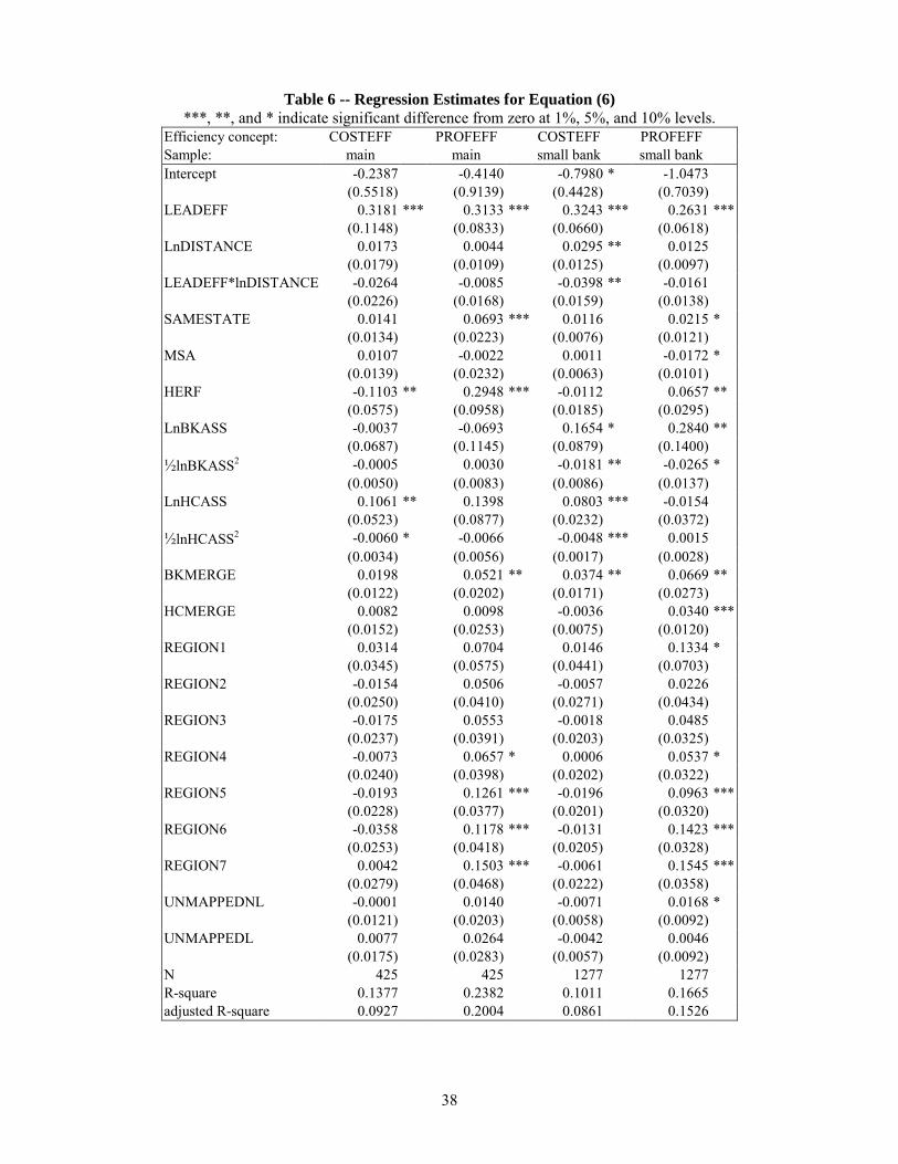
38

Table 6 -- Regression Estimates for Equation (6) ***, **, and * indicate significant difference from zero at 1%, 5%, and 10% levels.

Efficiency concept: COSTEFF PROFEFF COSTEFF PROFEFF Sample: main main small bank small bank Intercept -0.2387 -0.4140 -0.7980 * -1.0473

(0.5518) (0.9139) (0.4428) (0.7039) LEADEFF 0.3181 *** 0.3133 *** 0.3243 *** 0.2631 ***

(0.1148) (0.0833) (0.0660) (0.0618) LnDISTANCE 0.0173 0.0044 0.0295 ** 0.0125

(0.0179) (0.0109) (0.0125) (0.0097) LEADEFF*lnDISTANCE -0.0264 -0.0085 -0.0398 ** -0.0161

(0.0226) (0.0168) (0.0159) (0.0138) SAMESTATE 0.0141 0.0693 *** 0.0116 0.0215 *

(0.0134) (0.0223) (0.0076) (0.0121) MSA 0.0107 -0.0022 0.0011 -0.0172 *

(0.0139) (0.0232) (0.0063) (0.0101) HERF -0.1103 ** 0.2948 *** -0.0112 0.0657 ** (0.0575) (0.0958) (0.0185) (0.0295) LnBKASS -0.0037 -0.0693 0.1654 * 0.2840 **

(0.0687) (0.1145) (0.0879) (0.1400) ½lnBKASS2 -0.0005 0.0030 -0.0181 ** -0.0265 *

(0.0050) (0.0083) (0.0086) (0.0137) LnHCASS 0.1061 ** 0.1398 0.0803 *** -0.0154

(0.0523) (0.0877) (0.0232) (0.0372) ½lnHCASS2 -0.0060 * -0.0066 -0.0048 *** 0.0015

(0.0034) (0.0056) (0.0017) (0.0028) BKMERGE 0.0198 0.0521 ** 0.0374 ** 0.0669 ** (0.0122) (0.0202) (0.0171) (0.0273) HCMERGE 0.0082 0.0098 -0.0036 0.0340 ***

(0.0152) (0.0253) (0.0075) (0.0120) REGION1 0.0314 0.0704 0.0146 0.1334 *

(0.0345) (0.0575) (0.0441) (0.0703) REGION2 -0.0154 0.0506 -0.0057 0.0226

(0.0250) (0.0410) (0.0271) (0.0434) REGION3 -0.0175 0.0553 -0.0018 0.0485

(0.0237) (0.0391) (0.0203) (0.0325) REGION4 -0.0073 0.0657 * 0.0006 0.0537 *

(0.0240) (0.0398) (0.0202) (0.0322) REGION5 -0.0193 0.1261 *** -0.0196 0.0963 ***

(0.0228) (0.0377) (0.0201) (0.0320) REGION6 -0.0358 0.1178 *** -0.0131 0.1423 ***

(0.0253) (0.0418) (0.0205) (0.0328) REGION7 0.0042 0.1503 *** -0.0061 0.1545 ***

(0.0279) (0.0468) (0.0222) (0.0358) UNMAPPEDNL -0.0001 0.0140 -0.0071 0.0168 *

(0.0121) (0.0203) (0.0058) (0.0092) UNMAPPEDL 0.0077 0.0264 -0.0042 0.0046

(0.0175) (0.0283) (0.0057) (0.0092) N 425 425 1277 1277 R-square 0.1377 0.2382 0.1011 0.1665 adjusted R-square 0.0927 0.2004 0.0861 0.1526

39

Table 7 Evaluating ����NONLEADEFF/����LEADEFF as mean DISTANCE increases.

***, **, and * indicate significant difference from zero at 1%, 5%, and 10% levels. Efficiency concept: COSTEFF PROFEFF COSTEFF PROFEFF Sample: Main main small bank Small bank minimum DISTANCE in sample: 0 miles 0 miles 0 miles 0 miles point estimate of derivative 0.3182 *** 0.3133 *** 0.3243 *** 0.2631 ***standard error of derivative 0.1148 0.0833 0.0666 0.0618 banks in same state: 73 miles 73 miles 81 miles 81 miles point estimate of derivative 0.2053 *** 0.2769 *** 0.1499 *** 0.1925 ***standard error of derivative 0.0532 0.0441 0.0323 0.0298 banks in same region, different states: 288 miles 288 miles 188 miles 188 miles point estimate of derivative 0.1688 *** 0.2652 *** 0.1161 *** 0.1789 ***standard error of derivative 0.0591 0.0503 0.0387 0.0342 banks in contiguous regions: 597 miles 597 miles 368 miles 368 miles point estimate of derivative 0.1495 ** 0.2590 *** 0.0893 * 0.1680 ***standard error of derivative 0.0681 0.0573 0.0461 0.0399 banks in noncontiguous regions: 1297 miles 1297 miles 1278 miles 1278 miles point estimate of derivative 0.1495 ** 0.2590 *** 0.0893 * 0.1680 ***standard error of derivative 0.0681 0.0573 0.0461 0.0399 maximum DISTANCE in sample: 2825 miles 2825 miles 3303 miles 3303 miles point estimate of derivative 0.1084 0.2458 *** 0.0018 0.1327 ** standard error of derivative 0.0942 0.0767 0.0757 0.0645

Figure 1Derivative of affiliate bank efficiency (NONLEADEFF) with respect to

lead bank efficiency (LEADEFF). Based on Table 4 regression estimates.

0.00

0.05

0.10

0.15

0.20

0.25

0.30

0.35

0.40

0 500 1000 1500 2000 2500 3000 3500miles from affiliate bank to lead bank

�N

ON

LEA

DEF

F/�LE

AD

EFF

main sample, PROFEFFsmall bank sample, PROFEFFmain sample, COSTEFFsmall bank sample, COSTEFF

40

Table 8

Selected Regression Results for Subsample Estimates of Equation (6) ***, **, and * indicate significant difference from zero at 1%, 5%, and 10% levels.

dependent variable: COSTEFF PROFEFF COSTEFF PROFEFF sample: main main small bank small bank (a) full sample: LEADEFF 0.1996 *** 0.2774 *** 0.1760 *** 0.1996 ***

(0.0530) (0.0441) (0.0308) (0.0291) lnDISTANCE -0.0031 0.0005 -0.0018 0.0015

(0.0031) (0.0052) (0.0016) (0.0026) N 425 425 1277 1277 R-square 0.1348 0.2552 0.0966 0.1656 Adjusted R-square 0.0919 0.2183 0.0822 0.1524 (b) out-of-state affiliates only: LEADEFF 0.1098 0.3898 *** 0.0759 0.0840

(0.0903) (0.0725) (0.0843) (0.0786) lnDISTANCE -0.0037 -0.0420 ** -0.0128 * -0.0015

(0.0108) (0.0168) (0.0073) (0.0135) N 207 207 244 244 R-square 0.0931 0.2697 0.1181 0.2303 Adjusted R-square -0.0045 0.1912 0.0390 0.1612 (c) out-of-region affiliates only: LEADEFF 0.1400 0.5008 *** 0.2748 ** 0.4002 ***

(0.1390) (0.1123) (0.1152) (0.1072) lnDISTANCE -0.0063 -0.0492 * -0.0266 ** -0.0145

(0.0163) (0.0267) (0.0106) (0.0195) N 113 113 127 127 R-square 0.1893 0.3556 0.3184 0.3793 Adjusted R-square 0.0130 0.2156 0.1973 0.2690 (d) noncontiguous region affiliates only: LEADEFF 0.6325 0.9141 *** 0.5471 0.6042

(0.4288) (0.1389) (0.5674) (0.6298) lnDISTANCE 0.0007 0.1189 0.0878 0.2562

(0.0760) (0.0874) (0.0862) (0.4075) N 31 31 25 25 R-square 0.5258 0.8963 0.8477 0.6949 Adjusted R-square -0.0162 0.7778 0.5938 0.1864

41

Table 9.1 Cost Efficiency, Individual Organization Analysis

Data for banks in 33 BHCs that own at least 10 affiliate banks, ordered by the mean cost efficiency of those affiliates. "Statewide" BHCs only own affiliates in their home states. "Regional" BHCs own affiliates outside their home states, but not beyond their home regions. "Superregional, contiguous" BHCs own affiliates outside their home regions, but not beyond regions that are contiguous to the BHC. "Superregional, noncontiguous" BHCs own affiliates outside their home regions, including regions that are not contiguous to the BHC. The superscript A indicates a mean cost efficiency greater than 0.7989, which is the mean COSTEFF for all affiliates of multi-bank holding companies in our data. The superscript B indicates a BHC whose affiliates have mean cost efficiencies greater than 0.7989 in each of the geographic locations in which it operates.

Mean cost efficiency for banks located in:

(1)

Geographic scope of BHC

(2)

Number of banks in BHC

(3)

Mean cost efficiency

for all banks in BHC:

(4) home

state of BHC

(5) home region (but not in home state)

of BHC

(6) regions

contiguous to BHC

(7) regions not contiguous

to BHC

superregional, contiguous B 21 .9295 .9274 A .9721 A statewide B 13 .9027 .9027 A

superregional, contiguous B 15 .8987 .8979 A .8341 A .9232 A superregional, contiguous B 15 .8908 .9097 A .8355 A .8648 A superregional, contiguous B 16 .8822 .8089 A .8699 A .8989 A

superregional, noncontiguous 26 .8733 .8772 A .7775 statewide B 10 .8683 .8683 A

superregional, noncontiguous 27 .8639 .8734 A .6167 superregional, contiguous 15 .8601 .8662 A .7750

statewide B 10 .8356 .8356 A superregional, noncontiguous B 34 .8349 .8087 A .8784 A .8283 A .8598 A

regional B 28 .8285 .8181 A .8343 A regional B 10 .8275 .8041 A .8509 A

superregional, contiguous B 10 .8255 .8073 A .9893 A superregional, noncontiguous 13 .8240 .8890 A .8192 A .6613 .7643

superregional, contiguous 12 .8215 .8339 A .7918 .8388 A superregional, contiguous 10 .8207 .7146 .8995 A .8528 A

regional B 12 .8140 .8221 A .8114 A superregional, contiguous 13 .9132 .8093 A .7904 .8539 A

superregional, noncontiguous 12 .9126 .8688 A .8291 A .8714 A .6479 superregional, noncontiguous 20 .8103 .8205 A .7077 .9006 A .7681

superregional, contiguous 15 .8029 .7906 .8451 A .7823 superregional, contiguous 21 .7995 .8198 A .6681 .7279

statewide B 13 .7994 .7994 A superregional, contiguous 22 .7974 .8006 A .8051 A .7262 superregional, contiguous 10 .7889 .7946 .7659 superregional, contiguous 10 .7882 .7782 .8786 A

regional 35 .7834 .7655 .8138 A superregional, contiguous 13 .7829 .8808 A .7626 .7914

statewide 10 .7745 .7745 superregional, contiguous 11 .7675 .7613 .7751 superregional, contiguous 12 .7494 .7515 .6987 .7980 superregional, contiguous 10 .7387 .7416 .7152 .7493

42

Table 9.2 Profit Efficiency, Individual Organization Analysis

Data for banks in 33 BHCs that own at least 10 affiliate banks, ordered by the mean profit efficiency of those affiliates. "Statewide" BHCs only own affiliates in their home states. "Regional" BHCs own affiliates outside their home states, but not beyond their home regions. "Superregional, contiguous" BHCs own affiliates outside their home regions, but not beyond regions that are contiguous to the BHC. "Superregional, noncontiguous" BHCs own affiliates outside their home regions, including regions that are not contiguous to the BHC. The superscript A indicates a mean profit efficiency greater than 0.6931, which is the mean PROFEFF for all affiliates of multi-bank holding companies in our data. The superscript B indicates a BHC whose affiliates have mean profit efficiencies greater than 0.6931 in each of the geographic locations in which it operates.

Mean profit efficiency for banks located in:

(1)

Geographic scope of BHC

(2)

Number of banks in BHC

(3)

Mean profit efficiency

for all banks in BHC:

(4) home

state of BHC

(5) home region (but not in home state)

of BHC

(6) regions

contiguous to BHC

(7) regions not contiguous

to BHC

superregional, contiguous 21 .9051 .9173 A .6603 superregional, contiguous 15 .8448 .8944 A .6368 .8178 A

regional B 35 .8036 .8008 A .8084 A superregional, noncontiguous B 34 .7892 .7281 A .7794 A .8242 A .6999 A

statewide B 10 .7858 .7848 A superregional, contiguous 16 .7828 .6891 .9040 A .7667 A

superregional, noncontiguous B 26 .7746 .7697 A .8973 A superregional, contiguous B 13 .7648 .7303 A .8824 A .8021 A

superregional, noncontiguous 12 .7449 .8168 A .7622 A .7149 A .6512 statewide B 13 .7419 .7419 A regional B 12 .7308 .7231 A .7333 A

superregional, contiguous 12 .7278 .6709 .6566 .8564 A superregional, contiguous 13 .7231 .6395 .7370 A .7514 A

regional B 28 .7166 .7304 A .7089 A superregional, contiguous B 11 .7129 .7264 A .6966 A

superregional, noncontiguous 13 .7121 .6819 .8406 A .6985 A .7025 A superregional, contiguous 22 .7110 .7182 A .7065 A .5725 superregional, contiguous 21 .7105 .7269 A .7160 A .6150 superregional, contiguous 10 .7006 .7007 A .7227 A .6817

superregional, noncontiguous 20 .6939 .5153 .7342 A .7125 A .7348 A superregional, contiguous 10 .6920 .6931 .6875 superregional, contiguous 15 .6909 .7299 A .5184 .6058

statewide 10 .6861 .6861 regional 10 .6791 .6578 .7005 A

superregional, contiguous 10 .6662 .6693 .6389 superregional, contiguous 15 .6642 .6433 .6693 .6958 A superregional, contiguous 15 .6197 .6331 .8823 A superregional, contiguous 10 .6462 .6439 .6667 superregional, contiguous 10 .6349 .6872 .7585 A .4654 superregional, contiguous 12 .6238 .5603 .6161 .6952 A

statewide 10 .6166 .6166 statewide 13 .5847 .5847

superregional, noncontiguous 27 .5644 .5671 .4947