Embed Size (px)
Citation preview
THE EFFECTS OF DISTRIBUTED GENERATION SOURCES WITHIN
COMMERCIAL RETAIL RETICULATION NETWORKS
by
Justin Trevor Lotter
Submitted in partial fulfilment of the requirements for the degree
Master of Engineering (Electrical Engineering)
in the
Department of Electrical, Electronic and Computer Engineering
Faculty of Engineering, Built Environment and Information Technology
UNIVERSITY OF PRETORIA
January 2019
SUMMARY
THE EFFECTS OF DISTRIBUTED GENERATION SOURCES WITHIN
COMMERCIAL RETAIL RETICULATION NETWORKS
by
Justin Trevor Lotter
Supervisor: Dr R. Naidoo
Department: Electrical, Electronic and Computer Engineering
University: University of Pretoria
Degree: Master of Engineering (Electrical Engineering)
Keywords: Distributed generation, load parameters, photovoltaic systems,
reticulation network.
There is an increased implementation of renewable energy generation sources, such as solar
PV, within electrical networks. This is due to the reduced cost of electricity generated from
renewable energy systems as well as the world becoming more environmentally aware.
There is therefore a need to understand the effects of Distributed Generation (DG) within
commercial retail reticulation networks on load and networks parameters, such as coincident
demand and load factor. These load parameters play an important role in network design as
well as in load forecasting which influences network expansion and generation planning
decisions.
A hypothetical study was conducted on a low-voltage commercial retail reticulation network
to determine the effects of varying levels of DG penetration on load and network parameters.
Two DG placement scenarios were investigated; centrally and de-centrally located within
the reticulation network. Results from the hypothetical study were confirmed by conducting
the same analysis on a commercial retail reticulation network in service, with measured load
demand data available.

Results obtained indicated that load parameters such as coincident demand, load factor and
diversity factor are significantly impacted at high levels of DG penetration. Further
investigation is required to determine if the altering of load parameters, from the introduction
of DG would require current design procedures or standards to be modified and updated; or
if the standards applicable to the design of reticulation networks are still relevant when
varying levels of DG penetration are introduced.

LIST OF ABBREVIATIONS
ADMD After Diversity Maximum Demand
ANM Active Network Management
AVC Automatic Voltage Control
DG Distributed Generation
DMS Distribution Management System
DNOs Distribution Network Operators
GOP Garsfontein Office Park
GPS Global Positioning System
HV High-voltage
ICAE International Conference on Applied Energy
IEEE Institute of Electrical and Electronic Engineers
IPSO Improved Particle Swam Optimisation
LV Low-voltage
PSO Particle Swam Optimisation
PV Photovoltaic
RTU Remote Terminal Unit
SANS South African National Standards
SCADA Supervisory Control and Data Acquisition
SLD Single Line Diagram
USA United States of America
TABLE OF CONTENTS
CHAPTER 1 INTRODUCTION .....................................................................1
1.1 PROBLEM STATEMENT ....................................................................................1
1.1.1 Context of the problem ................................................................................1
1.1.2 Research gap ...............................................................................................2
1.2 RESEARCH OBJECTIVE AND QUESTIONS ....................................................4
1.3 APPROACH .........................................................................................................4
1.3.1 Hypothetical study ......................................................................................4
1.3.2 Case study ...................................................................................................6
1.4 RESEARCH GOALS ............................................................................................6
1.5 RESEARCH CONTRIBUTION ............................................................................6
1.6 RESEARCH OUTPUTS .......................................................................................7
1.7 DISSERTATION OVERVIEW .............................................................................7
CHAPTER 2 LITERATURE STUDY .............................................................9
2.1 CHAPTER OVERVIEW .......................................................................................9
2.2 HOW DISTRIBUTED GENERATION IS CHANGING NETWORK
TOPOLOGIES ......................................................................................................9
2.2.1 Smart grids ................................................................................................ 10
2.2.2 Micro-grids ............................................................................................... 10
2.3 EFFECTS OF DISTRIBUTED GENERATION ON TECHNICAL NETWORK
PARAMETERS .................................................................................................. 11
2.3.1 Minimise losses ......................................................................................... 11
2.3.2 Voltage profile improvement ..................................................................... 12
2.3.3 Network fault levels .................................................................................. 14
2.3.4 Protection strategies .................................................................................. 15
2.3.5 Power system stability ............................................................................... 18
2.3.6 Effect on power system operation .............................................................. 19
2.3.7 Economic benefits of distributed generation .............................................. 21
2.4 CHAPTER SUMMARY ..................................................................................... 22
CHAPTER 3 HYPOTHETICAL STUDY ..................................................... 24
3.1 CHAPTER OVERVIEW ..................................................................................... 24
3.2 NETWORK MODEL INPUT PARAMETERS ................................................... 24
3.2.1 Load modelling ......................................................................................... 24
3.2.2 Suitable DG source ................................................................................... 29
3.2.3 Reticulation network model ....................................................................... 30
3.2.4 Analysis .................................................................................................... 32
3.3 BASE CASE SCENARIO RESULTS ................................................................. 33
3.3.1 Load parameter definitions ........................................................................ 34
3.3.2 Load parameters ........................................................................................ 35
3.3.3 Network parameters .................................................................................. 37
3.4 CENTRALISED DG SCENARIO RESULTS ..................................................... 37
3.4.1 Load parameters ........................................................................................ 39
3.4.2 Network parameters .................................................................................. 41
3.5 DE-CENTRALISED DG SCENARIO RESULTS ............................................... 43
3.5.1 Load parameters ........................................................................................ 44
3.5.2 Network parameters .................................................................................. 46
3.6 CHAPTER SUMMARY ..................................................................................... 47
CHAPTER 4 CASE STUDY .......................................................................... 48
4.1 CHAPTER OVERVIEW ..................................................................................... 48
4.2 METERED LOAD DATA AND EXISTING RETICULATION NETWORK
INFORMATION ................................................................................................. 48
4.2.1 Load modelling ......................................................................................... 49
4.2.2 Reticulation network ................................................................................. 52
4.3 MODELLING OF DG SOURCE ........................................................................ 54
4.4 BASE CASE SCENARIO RESULTS ................................................................. 56
4.4.1 January 2017 load demand scenario........................................................... 56
4.4.2 July 2016 load demand scenario ................................................................ 59
4.5 CENTRALISED DG SCENARIO RESULTS ..................................................... 61
4.5.1 January 2017 load demand scenario........................................................... 62
4.5.2 July 2016 load demand scenario ................................................................ 66
4.6 DE-CENTRALISED DG SCENARIO RESULTS ............................................... 70
4.6.1 January 2017 load demand scenario........................................................... 70
4.6.2 July 2016 load demand scenario ................................................................ 75
4.7 CHAPTER SUMMARY ..................................................................................... 79
CHAPTER 5 DISCUSSION ........................................................................... 81
5.1 CHAPTER OVERVIEW ..................................................................................... 81
5.2 HYPOTHETICAL STUDY................................................................................. 81
5.2.1 Load parameters ........................................................................................ 81
5.2.2 Network parameters .................................................................................. 95
5.3 CASE STUDY .................................................................................................... 96
5.3.1 Load parameters ........................................................................................ 96
5.3.2 Network parameters ................................................................................ 111
5.4 SUMMARY ...................................................................................................... 113
CHAPTER 6 CONCLUSION ...................................................................... 115
REFERENCES ................................................................................................ 118
LIST OF FIGURES
Figure 3.1. Normalised commercial retail customer hourly load demand profile .............. 28
Figure 3.2. Normalised solar PV generation profile ......................................................... 29
Figure 3.3. Hypothetical commercial retail reticulation network single line diagram ....... 33
Figure 3.4. Base case load demand profile ....................................................................... 36
Figure 3.5. Base case transformer percentage loading ...................................................... 36
Figure 3.6. Base case supply voltage profile .................................................................... 37
Figure 3.7. Single line diagram with central DG source ................................................... 38
Figure 3.8. Coincident load demand versus DG penetration............................................. 39
Figure 3.9. Transformer percentage loading versus DG penetration ................................. 40
Figure 3.10. Supply voltage profile versus DG penetration .............................................. 42
Figure 3.11. Single line diagram with de-central DG source ............................................ 43
Figure 3.12. Coincident load demand versus de-central DG penetration .......................... 44
Figure 3.13. Customer No. 5 low-voltage feeder percentage loading versus DG penetration
........................................................................................................................................ 45
Figure 3.14. Customer no. 5 supply voltage profile versus DG penetration ...................... 46
Figure 4.1. Case study reticulation network single line diagram....................................... 54
Figure 4.2. Base case load demand profile (Jan 2017 load demand data) ......................... 57
Figure 4.3. Base case transformer percentage loading (Jan 2017 load demand data) ........ 58
Figure 4.4. Base case supply voltage profile (Jan 2017 load demand data)....................... 58
Figure 4.5. Base case load demand profile (July 2016 load demand data) ........................ 60
Figure 4.6. Base case transformer percentage loading (July 2016 load demand data) ....... 60
Figure 4.7. Base case supply voltage profile (July 2016 load demand data) ..................... 61
Figure 4.8. Case study central DG scenario single line diagram ....................................... 62
Figure 4.9. Coincident load demand versus DG penetration (Jan 2017 load demand)....... 63
Figure 4.10. Transformer percentage loading versus DG penetration (Jan 2017 load
demand) ........................................................................................................................... 63
Figure 4.11. Supply voltage profile versus DG penetration (Jan 2017 load demand) ........ 65
Figure 4.12. Coincident load demand versus DG penetration (July 2016 load demand) ... 67
Figure 4.13. Transformer percentage loading versus DG penetration (July 2016 load
demand) ........................................................................................................................... 67
Figure 4.14. Supply voltage profile versus DG penetration (July 2016 load demand)....... 69
Figure 4.15. Single line diagram with de-central DG source (case study) ......................... 70
Figure 4.16. Coincident load demand versus de-central DG penetration (Jan 2017 load
demand) ........................................................................................................................... 71
Figure 4.17. Transformer percentage loading versus de-central DG penetration (Jan 2017
load demand) ................................................................................................................... 72
Figure 4.18. DB-M3 feeder cable percentage loading versus DG penetration (Jan 2017) . 72
Figure 4.19. DB-M3 supply voltage profile versus DG penetration (Jan 2017) ................ 74
Figure 4.20. Coincident load demand versus de-central DG penetration (July 2016 load
demand) ........................................................................................................................... 76
Figure 4.21. Transformer percentage loading versus de-central DG penetration (July 2016
load demand) ................................................................................................................... 76
Figure 4.22. DB-M3 feeder cable percentage loading versus DG penetration (July 2016) 77
Figure 4.23. DB-M3 supply voltage profile versus DG penetration (July 2016) ............... 78
Figure 5.1. Coincident demand versus DG penetration (hypothetical study, central DG) . 82
Figure 5.2. Coincident demand versus DG penetration (hypothetical study, de-central DG)
........................................................................................................................................ 83
Figure 5.3. Demand factor versus DG penetration (hypothetical study, central DG) ........ 84
Figure 5.4. Demand factor versus DG penetration (hypothetical study, de-central DG).... 85
Figure 5.5. Utilisation factor versus DG penetration (hypothetical study, central DG) ..... 86
Figure 5.6. Utilisation factor versus DG penetration (hypothetical study, de-central DG) 87
Figure 5.7. Load factor versus DG penetration (hypothetical study, central DG) .............. 88
Figure 5.8. Load factor versus DG penetration (hypothetical study, de-central DG) ......... 89
Figure 5.9. Diversity factor versus DG penetration (hypothetical study, central DG) ....... 90
Figure 5.10. Coincidence factor versus DG penetration (hypothetical study, central DG) 90
Figure 5.11. Diversity factor versus DG penetration (hypothetical study, de-central DG) 91
Figure 5.12. Coincidence factor versus DG penetration (hypothetical study, de-central
DG) ................................................................................................................................. 91
Figure 5.13. Load diversity versus DG penetration (hypothetical study, central DG) ....... 92
Figure 5.14. Load diversity versus DG penetration (hypothetical study, de-central DG) .. 93
Figure 5.15. Loss factor versus DG penetration (hypothetical study, central DG) ............ 94
Figure 5.16. Loss factor versus DG penetration (hypothetical study, de-central DG) ....... 94
Figure 5.17. Minimum and maximum supply voltage versus DG penetration (hypothetical
study, central DG) ............................................................................................................ 95
Figure 5.18. Minimum and maximum supply voltage versus DG penetration (hypothetical
study, de-central DG) ....................................................................................................... 96
Figure 5.19. Coincident demand versus DG penetration (case study, central DG) ............ 97
Figure 5.20. Coincident demand versus DG penetration (case study, de-central DG) ....... 98
Figure 5.21. Demand factor versus DG penetration (case study, central DG) ................... 99
Figure 5.22. Demand factor versus DG penetration (case study, de-central DG) ............ 100
Figure 5.23. Utilisation factor versus DG penetration (case study, central DG) .............. 101
Figure 5.24. Utilisation factor versus DG penetration (case study, de-central DG) ......... 102
Figure 5.25. Load factor versus DG penetration (case study, central DG) ...................... 103
Figure 5.26. Load factor versus DG penetration (case study, de-central DG) ................. 104
Figure 5.27. Diversity factor versus DG penetration (case study, central DG) ................ 105
Figure 5.28. Coincidence factor versus DG penetration (case study, central DG) ........... 106
Figure 5.29. Diversity factor versus DG penetration (case study, de-central DG) ........... 107
Figure 5.30. Coincidence factor versus DG penetration (case study, de-central DG) ...... 107
Figure 5.31. Load diversity versus DG penetration (case study, central DG) .................. 108
Figure 5.32. Load diversity versus DG penetration (case study, de-central DG) ............. 109
Figure 5.33. Loss factor versus DG penetration (case study, central DG) ....................... 110
Figure 5.34. Loss factor versus DG penetration (case study, de-central DG) .................. 111
Figure 5.35. Minimum and maximum supply voltage versus DG penetration (case study,
central DG) .................................................................................................................... 112
Figure 5.36. Minimum and maximum feeder voltage versus DG penetration (case study,
de-central DG) ............................................................................................................... 113
LIST OF TABLES
Table 3.1 Commercial static load model parameters ........................................................ 26
Table 3.2 Commercial static load model parameters ........................................................ 28
Table 3.3 Supply transformer parameters......................................................................... 31
Table 3.4 Feeder cable parameters ................................................................................... 32
Table 3.5 Customer feeder cable length ........................................................................... 32
Table 3.6 Definitions and formula of load parameters under investigation ....................... 34
Table 3.7 Base case (No DG source integrated) load parameter results ............................ 35
Table 3.8 Solar PV penetration levels and capacities modelled ........................................ 38
Table 3.9 External load parameters versus percentage DG penetration for central scenario
........................................................................................................................................ 40
Table 3.10 Supply voltage maximum and minimum level for varying levels of DG
penetration ....................................................................................................................... 42
Table 3.11 De-centralised DG penetration levels and capacities modelled ....................... 44
Table 3.12 External load parameters versus percentage DG penetration for de-central
scenario ........................................................................................................................... 45
Table 3.13 Customer no. 5 supply voltage maximum and minimum level for varying levels
of DG penetration ............................................................................................................ 47
Table 4.1 Unit numbers, description and meter numbers for each customer ..................... 50
Table 4.2 Reticulation network cables properties and lengths .......................................... 53
Table 4.3 Step-down transformer properties .................................................................... 53
Table 4.4 Centralised DG penetration levels and capacities modelled (Jan 2017 scenario)
........................................................................................................................................ 55
Table 4.5 Centralised DG penetration levels and capacities modelled (July 2016 scenario)
........................................................................................................................................ 55
Table 4.6 Base case (January 2017) load parameter results .............................................. 56
Table 4.7 Base case (July 2016) load parameter results .................................................... 59
Table 4.8 Load parameters versus percentage DG penetration (Jan 2017 load demand) ... 64
Table 4.9 Supply voltage for varying levels of DG penetration (Jan 2017 load demand) .. 66
Table 4.10 Load parameters versus percentage DG penetration (July 2016 load demand) 68
Table 4.11 Supply voltage for varying levels of DG penetration (July 2016 load demand)
........................................................................................................................................ 69
Table 4.12 De-centralised DG penetration levels and capacities modelled ....................... 71
Table 4.13 Load parameters versus percentage DG penetration for de-central scenario (Jan
2017) ............................................................................................................................... 73
Table 4.14 DB-M3 supply voltage for varying levels of DG penetration (January 2017) .. 75
Table 4.15 Load parameters versus percentage DG penetration for de-central scenario
(July 2016) ....................................................................................................................... 77
Table 4.16 DB-M3 supply voltage for varying levels of DG penetration (July 2016) ....... 79
CHAPTER 1 INTRODUCTION
1.1 PROBLEM STATEMENT
1.1.1 Context of the problem
Distributed Generation (DG) is defined as “an electric power source connected directly to
the distribution network or on the customer side of the meter” [1]. Renewable energy DG
sources are becoming increasingly utilised as electricity consumers globally become more
environmentally conscious. Another factor that has contributed to the increased
implementation of renewable energy DG sources is the decreased cost of electricity
generation from sources such as wind and solar Photovoltaic (PV) system, as a result of the
advance in technology [2].
Distribution networks are typically planned, designed and operated to be purely passive
networks that deliver electricity to consumers in a unidirectional manner (from source to
load) with minimal or no monitoring and control capabilities [3]. The introduction of DG
into distribution networks alters conventional power flow within the network [4], and can
results in bi-directional power flow [4]. This has an impact on load parameters of the
composite load (as seen from the external grid) and network parameters within the network.
A significant number of assumptions are made in order to determine suitable parameters
used to predict the future load demands [5]. Understanding how load parameters are effected,
from the addition of DG, is therefore important for predicting future load demands with DG
sources present.
CHAPTER 1 INTRODUCTION
Department of Electrical, Electronic and Computer Engineering 2
University of Pretoria
Load forecasting utilises a combination of the load parameters such as diversity factor, load
factor, load demand profile, loss factor, growth rate and after diversity maximum demand
(ADMD) [5]. Altering of any of these parameters from the introduction of DG can have an
impact on planning and design of electrical networks [5].
The factors that define or impact the technical performance of an electrical distribution
network are electrical losses, voltage regulation, equipment loading and utilisation, system
fault levels, frequency and harmonics [6]. In contrast to distribution networks (typically
medium-voltage); when considering low-voltage reticulation networks (and the integration
of DG) only certain parameters need to be considered. These parameters are voltage, thermal
loading of equipment, peak load demand, network losses as well as feeder protection [7].
1.1.2 Research gap
Understanding how load and network parameters are affected from the introduction of DG
is important for many reasons. Altering of load parameters affects how reticulation networks
are planned, designed and operated. Altering of load parameters can also affect load demand
forecasting, which plays a critical role in transmission and distribution network planning. By
analysis of load and network parameters at varying levels of DG penetration, the effect on
load parameters, such as coincident demand, diversity factor and load factor can be
determined.
A significant amount of research has been conducted regarding the optimal placement of DG
within distribution networks to improve network parameters such as energy losses and
voltage profiles; as well as a comparison of different optimisation techniques [3], [4], [6],
[8] - [14].
Another area in which a significant amount of research has been conducted is with regards
to network protection strategies for networks containing DG, implications of introducing DG
into existing distribution networks on network protection and improved network protection
CHAPTER 1 INTRODUCTION
Department of Electrical, Electronic and Computer Engineering 3
University of Pretoria
schemes to increase DG penetration levels without comprising system performance [15] -
[21].
Although the body of knowledge surrounding the integration of DG into distribution
networks is vast, there is little focus on reticulation networks (low-voltage networks); in
particular, on how the integration of DG into commercial retail reticulation networks affects
load parameters.
Limited research has been conducted in this area; however, research on technical behaviour
of low-voltage networks with varied levels of renewable penetration has been conducted [7].
The focus of this research was primarily on the effects of DG on voltage profiles and
networks losses. Although relevant, the focus of the particular research did not cover the
impact of DG on load parameters. The impact of DG on ADMD or coincident demand has
been investigated [5]; however, not all load parameters which are under consideration in this
research were investigated. Refer to section 3.3.1 for the definitions and formulas for the
eight load parameters under investigation for this study.
The effect of varying levels of DG penetration for low-voltage networks has been analysed,
with regards to voltage profile improvement. It was found that an improvement in the voltage
profile was the most considerable when load demand profiles match with the energy
generation source profile [7]. It was also found that if there was a mismatch between the
energy generation source profile and load demand, there was not a reduction in network peak
demand [7]. Although this information is valuable and could provide insight on how to plan
or design a network that would include DG, there was no focus on the effects of DG on the
different load parameters. The effects on load parameters provides insight into load
behaviour which is of great importance during network planning and design.
Based on the fact that there has been limited research conducted on the impact of DG on
load and network parameters within commercial retail reticulation networks, there is a clear
research gap in the body of knowledge surrounding the topic. Further research is required to
gain a better understanding of how load parameters, for the composite commercial retail
CHAPTER 1 INTRODUCTION
Department of Electrical, Electronic and Computer Engineering 4
University of Pretoria
load, are impacted by the introduction of varying levels of DG into the commercial
reticulation network.
1.2 RESEARCH OBJECTIVE AND QUESTIONS
The objective of the research was to determine how DG effects load parameters (as seen by
the external network) and network parameters within the reticulation network, when
integrated into commercial retail reticulation networks.
The research question addressed was how the introduction of DG into commercial retail
reticulation networks would affect load and network parameters. These effects could be used
to determine if current planning and design procedures or standards are adequate for the
design of reticulation networks containing varying levels of DG penetration. This topic is
beyond the scope of this study.
1.3 APPROACH
To determine the effects that the introduction of DG has on load and network parameters
within commercial retail reticulation networks, the research conducted was done in two
separate phases; namely, a hypothetical study and a case study. The hypothetical study was
based on assumed or publicly available information as well as a typical reticulation network
topology. The case study was based on actual information obtained for an existing
commercial retail facility. The research methodology applied for each phase is detailed in
section 1.3.1 and 1.3.2 respectively.
1.3.1 Hypothetical study
Many factors needed to be determined, or assumed based on common practice, before results
could be obtained for the hypothetical study. Developing the hypothetical study began with
load modelling and developing load demand profiles of each of the hypothetical consumers.
Once the load modelling was complete, a reticulation network model was developed.
CHAPTER 1 INTRODUCTION
Department of Electrical, Electronic and Computer Engineering 5
University of Pretoria
The reticulation network was based on an assumed network topology and component sizes,
such as transformer capacity and feeder cable sizes. Results obtained for the load parameters
and network parameters under consideration, for this research, were obtained for the scenario
with no DG integrated into the reticulation network. This is referred to as the base case
scenario and serves as the reference point for which all comparisons are made. Varying
levels of DG penetration (based on load demand) and integration points within the
reticulation network were then analysed.
The first DG integration scenario analysed was with a DG source introduced at the common
low-voltage busbar, of the step-down transformer which supplied all the customers. This
scenario is referred to as the central DG scenario. The second DG integration scenario,
referred to as the de-central DG scenario, introduced the DG source further down within the
network at a customer sub-distribution board level.
The DG source capacity in both scenarios was varied to a maximum of the coincident load
demand at the particular busbar it was connected to. The impact on load and network
parameters for the varying penetration levels and DG scenarios was then obtained and
analysed.
Modelling of the reticulation network was done using a suitable power system simulation
software package. There are many suitable software packages that could have been utilised
to perform the required simulation studies. The software package utilised was DIgSILENT
Power Factory1 software. The reason for the selection was primarily because DIgSILENT
Power Factory software was available and it has the required functionality to perform the
suitable simulation studies.
1 DIgSILENT Power Factory is a product of DIgSILENT GmbH
http://www.digsilent.de/index.php/products-powerfactory.html
CHAPTER 1 INTRODUCTION
Department of Electrical, Electronic and Computer Engineering 6
University of Pretoria
1.3.2 Case study
A similar approach to the hypothetical study was followed for the case study. To validate
the results obtained for the hypothetical study, a case study was conducted on a commercial
retail reticulation network with actual measured load demand data and information gathered
on the reticulation network in service. The information gathered from an on-site
investigation was used to develop the network model. The analysis of the impact of the two
different DG scenarios (central DG and de-central DG) on load and network parameters was
also conducted.
1.4 RESEARCH GOALS
The goal of this research was to determine the effects of varying levels of DG penetration
on load parameters (as seen by the external network) and network parameters within the
network. The results and outcome from this study could potentially be used to assess the
suitability of current design procedures and standards for reticulation networks that are
proposed to contain DG sources. The assessment of current planning standards and design
procedures, along with the findings of how DG affects load and networks parameters, will
provide insight into which aspects of planning standards or design procedures require
updating or improving. The assessment of current planning standards and design procedures
is beyond the scope of this study.
1.5 RESEARCH CONTRIBUTION
The contribution from the research was the identification and quantification of the effects of
varying levels of DG penetration on load and network parameters for commercial retail
reticulation networks. An extensive literature study indicated that, although research has
been conducted on the effects of DG on load parameters, the focus was on a single load
parameter, ADMD as opposed to multiple parameters. Further research was therefore
required to determine the effects of varying levels of DG penetration on all relevant load
parameters.
CHAPTER 1 INTRODUCTION
Department of Electrical, Electronic and Computer Engineering 7
University of Pretoria
The research has contributed to a better understanding of the effects of varying levels of DG
penetration on multiple load parameters. These parameters are of great importance in
network planning and design. The effect of varying levels of DG penetration on network
parameters, such as supply voltage, were also determined and quantified. This parameter
also plays a critical role in network planning and design.
1.6 RESEARCH OUTPUTS
From the research conducted for this study, an international conference paper was submitted
to the 9th International Conference on Applied Energy (ICEA) and accepted. The conference
paper was also published in the Energy Procedia, Volume 142.
1.7 DISSERTATION OVERVIEW
Chapter 2 presents the body of knowledge surrounding DG and the integration within
distribution networks. It was found that the integration of DG into distribution networks
poses many concerns but also has certain advantages. There are many factors that need to be
considered when integrating DG into distribution networks and these are further discussed
in chapter 2. Although the body of knowledge surrounding the integration of DG into
distribution networks is vast, the same cannot be said for reticulation networks.
Chapter 3 details the load models developed for the hypothetical study as well as the
associated reticulation network. Chapter 3 also presents the results obtained for hypothetical
study.
Chapter 4 provides information on the existing commercial retail reticulation network as
well as measured load demand data for all the customers assessed. Chapter 4 also details the
analysis and results obtained for the case study in order to validate the results obtained by
the hypothetical study.

CHAPTER 1 INTRODUCTION
Department of Electrical, Electronic and Computer Engineering 8
University of Pretoria
Chapter 5 provides a discussion and comparison of results obtained from both the
hypothetical study and the case study conducted.
Chapter 6 concludes the dissertation, summaries the findings and identifies further research
areas based on the findings.
CHAPTER 2 LITERATURE STUDY
2.1 CHAPTER OVERVIEW
The objective of this chapter is to provide a comprehensive overview of the body of
knowledge that surrounds DG, and in some cases, literature applicable to reticulation
networks containing DG sources. Section 2.2 discusses how network topologies are being
altered due to DG. Section 2.3 discusses the technical effects of DG on network parameters.
2.2 HOW DISTRIBUTED GENERATION IS CHANGING NETWORK
TOPOLOGIES
Traditional distribution networks were planned, designed, constructed and operated to be
purely passive systems and used to deliver electricity to consumers in a unidirectional
manner [3]. With the introduction of DG into a distribution network, conventional power
flow within the network is altered and can become bi-directional [4]. This influences how
networks should be planned, designed and operated so that the various impacts of the
introduction DG can be taken into account.
The factors that define the technical performance of an electrical network are electrical
losses, voltage regulation, equipment loading and utilisation, fault levels, stability limits,
frequency and harmonics [6]. Understanding how DG affects the technical performance of
the power system is key to being able to successfully plan, design and operate electrical
networks that contain DG sources in a safe and efficient manner.
CHAPTER 2 LITERATURE STUDY
Department of Electrical, Electronic and Computer Engineering 10
University of Pretoria
To address many of the issues involved with the integration of DG to the distribution
network, smart grids are being developed. The definition of a smart grid, according to the
Internal Energy Agency, is “an electricity network that uses digital technology to monitor
and manage the transport of electricity from all generation sources to meet the varying
electricity demand of the end user” [22].
2.2.1 Smart grids
Smart grids should be able to determine and co-ordinate the needs and capabilities of all
generation sources, grid operators, end users and electricity market stakeholders in such a
manner that they are able to optimise asset utilisation and operation as well as minimise both
costs and environmental impacts in the process, all whilst maintaining system reliability,
resilience and stability [22].
The introduction of DG requires distribution networks to move towards more intelligent
networks that can monitor and control generation sources so that they align with load
demands. This would then ensure the optimal use of DG, as well as electrical infrastructure,
between the generation sources and the end user.
2.2.2 Micro-grids
The introduction of DG sources can also alter networks on a smaller scale, other than
transmission or distribution networks. These small-scale networks are called micro-grids. A
micro-grid is defined as “a group of interconnected loads and distributed energy resources
within clearly defined electrical boundaries, that acts as a single controllable entity with
respects to the grid. A micro-grid can connect and disconnect from the grid to enable it to
operate in both grid-connected mode and island mode” [23]. The addition of DG results in
altering loads from passive uncontrollable entities to active controllable entities which has
its associated advantages and disadvantages. The impact of altering load characteristics then
needs to be determined in order to adequately plan and implement suitable electrical power
systems.
CHAPTER 2 LITERATURE STUDY
Department of Electrical, Electronic and Computer Engineering 11
University of Pretoria
2.3 EFFECTS OF DISTRIBUTED GENERATION ON TECHNICAL NETWORK
PARAMETERS
With an increase in the implementation of DG, there are many factors that need to be
considered when planning and designing electrical networks. These factors could either
enhance the network performance or be detrimental to the network performance. This is
dependent on many factors and can only be quantified on a case by case basis [4]. There are
a number of technical issues that need to be taken into account when connecting DG sources
to the distribution network, such as [24]:
• Thermal ratings of equipment;
• System fault levels;
• Stability;
• Reverse power flow capabilities of tap-changers;
• Line-drop compensation;
• Steady-state voltage rise;
• Network losses;
• Power quality (flicker and harmonics); and
• Network protection.
The effects of DG, on power systems, for each of the above-mentioned factors are further
described in sections 2.3.1 to 2.3.7.
2.3.1 Minimise losses
The optimal placement of DG can have the effect of reducing energy losses within the
network. This reduction of energy losses is achieved by reducing the current magnitudes that
flow within the distribution networks, which reduces the energy losses (I2R losses) within
the network. This would be the effect of integrating a DG source at the end of a radial
network and would reduce energy losses within the network. The current magnitudes are
reduced by reducing the load current that would need to be supplied via the distribution
CHAPTER 2 LITERATURE STUDY
Department of Electrical, Electronic and Computer Engineering 12
University of Pretoria
network. This results in a reduction of energy losses along the network. This is a simplified
scenario; however, the same cannot be assumed for more complex networks with multiple
nodes. To determine the placement of DG within complex networks, which would result in
minimal energy losses, requires optimisation. The optimisation can be achieved by making
use of different techniques, objective functions or system constraints.
One paper which explored the placement of DG employed a particle swarm optimisation
(PSO) technique focused on minimising real power losses in the primary distribution
networks [12]. Results for a 69-bus network were in close correlation to other optimisation
technique results obtained. PSO techniques could be further expanded to multi-objective
optimisation with a focus on reducing real power losses, improving voltage stability and
current balancing within certain sections of the power system within a radial distribution
system [14].
Optimal placement and sizing of DG using the improved particle swam optimisation (IPSO)
- monte carlo algorithm technique has been found to reduce active and reactive power losses,
improve voltage profiles and enhance system reliability [8].
Multi-objective optimisation, using PSO with an alternative proposed algorithm, focused on
the minimisation of power losses whilst simultaneously maximising voltage stability within
the system [9]. The optimisation yielded reduced power losses and improved voltage
stability by finding the bus within the network with the lowest voltage. The proposed
algorithm was compared to other analytical techniques and was found to perform better [9].
2.3.2 Voltage profile improvement
By altering the parameters within the distribution network, such as current, there can would
be effects noted on other system parameters such as voltage. System voltage is an important
parameter within distribution systems since distribution network operators (DNOs) are
required, by regulations, to maintain supply voltages within certain specified tolerances, i.e.
±5% of normal voltage. In weak networks voltage stability can often be a problem as system
CHAPTER 2 LITERATURE STUDY
Department of Electrical, Electronic and Computer Engineering 13
University of Pretoria
voltages may vary significantly as the loading of the network is increased, which could result
in voltage violations occurring.
By introducing DG into the network, loading of the network is altered during the periods of
generation. This would influence voltages within the distribution network. The influence on
voltage profiles within the network can be improved if DG is placed correctly within the
system [25]. To improve voltage profiles, optimal placement of DG must be done. This will
also help improve voltage rise or fluctuations within the system [26].
Optimisation, in terms of placement and sizing of DG, could be done by using the same
optimisation techniques used for minimising energy losses by implementing a different
objective function. One such technique is sensitivity analysis [27] and results obtained were
based on a new voltage stability index for optimal placement of DG in a radial system.
Another method for obtaining the optimal solution could be a combination of different
techniques such as sensitivity analysis and PSO. One example of such a methodology is a
combination of loss sensitivity factor, to determine the most optimal location for the DG
source, and PSO for optimising the capacity of the DG system to reduce total system losses,
as well as voltage improvements along a radial distribution system [10].
A hybrid algorithm between a genetic algorithm and PSO has been employed and yielded
results of reduced system energy losses, improved system voltage regulations as well as
improved system voltage stability [13]. Variations of PSO algorithms alone have also
demonstrated the ability to optimise DG placement in terms of improving voltage profiles
[9], [28].
Besides for several optimisation techniques available to improve voltage profiles or reduce
the effects of excessive voltage rise, due to DG integration, the following alternatives could
also be implemented [24]:
• Reduce primary substation voltage;
CHAPTER 2 LITERATURE STUDY
Department of Electrical, Electronic and Computer Engineering 14
University of Pretoria
• Allow the generation source to import reactive power;
• Install auto-transformers or voltage regulators along the line;
• Increase conductor size;
• Constrain the generation output at times of low demand; or
• A combination of the above.
The selection of the most appropriate scheme must be done on a site-by-site basis as each of
the above-mentioned schemes has its associated limitations [24].
Analysis of the effect of varying levels of DG penetration for low-voltage networks has been
conducted and found that voltage profile improvement was the most considerable when load
demand profiles match with the generation profile [7].
2.3.3 Network fault levels
Short-circuit fault level is an important parameter that needs to be considered when planning,
designing and operating power systems. Fault levels dictate equipment rating which ensures
that equipment can withstand the severe stresses that it experiences due to the high fault
currents that occur when a fault on an electrical network takes place. Fault levels within the
network could be altered and the direction of fault currents may change from the integration
of DG. A change in fault current magnitude or direction may negatively affect protection
devices if they are unable to respond in the manner which was originally intended, to safely
protect the network [29].
The fault contribution of a single small DG unit is not significant but it is very seldom that
a single DG unit is integrated into a distribution network. The cumulative contribution of
many DG units can alter network fault levels which can result in mis-coordination of
protection equipment [15]. Mis-coordination between protection devices is due to altering
of the fault currents [30]. False tripping of feeders, relay mal-operation, fuse-fuse mis-
coordination and fuse-recloser mis-coordination are common issues observed [21].
CHAPTER 2 LITERATURE STUDY
Department of Electrical, Electronic and Computer Engineering 15
University of Pretoria
It was also found that the introduction of DG downstream from a substation decreases the
fault contribution from the upstream substation [18]. This has an impact on the effectiveness
of the protection system upstream.
Despite the impacts of introducing DG into the distribution network, on system fault levels
and protection coordination, the effects are still dependent on the location of integration and
network topology into which the DG source is incorporated [18], [29].
2.3.4 Protection strategies
Distribution networks are conventionally radial in topology, and the protection strategies for
these networks assume a single-source of supply and single direction current flow within
branches [19]. Conventional protection strategies for radial distribution networks usually
take the form of overcurrent and time-current graded protection. These strategies are cost
effective and simple to coordinate and provide clear discrimination for fault currents
between protection devices [19].
The introduction of DG into a distribution network alters the network from a radial network
with a single source of supply to a radial network with multiple sources of supply. This
results in bi-directional power flow within the network [19]. Based on this, the conventional
distribution network is subjected to varying faults levels which further compromises
protection coordination [19].
Distribution network systems which have a high penetration levels of DG may exhibit poor
protection coordination and thus negatively impact system reliability [31]. Due to reduced
system reliability and safety concerns, more advanced protection schemes need to be
developed for such distribution systems.
Integration of DG into the distribution network can lead to various problems with regards to
the protection system namely [18];
CHAPTER 2 LITERATURE STUDY
Department of Electrical, Electronic and Computer Engineering 16
University of Pretoria
• False tripping of feeders;
• Nuisance tripping of generation plants;
• Blinding of protection relays;
• Increased or decreased fault levels;
• Unwanted islanding;
• Prohibition of automatic reclosing; and
• Unsynchronised reclosing.
False tripping occurs when a protection relay detects and opens its associated circuit breaker
based on a fault signal for a fault that has occurred in an unrelated network region [19]. The
cause of such false tripping is because of reverse current flowing from the downstream DG
source to the upstream faulted network [18]. To avoid false tripping, it is important to ensure
that proper protection coordination is achieved within power systems [18]. Distribution
networks typically make use of non-directional protection equipment and a change to
directionally sensitive protection equipment would eliminate false tripping due to the
introduction of DG [19].
‘Blinding’ of protection relays occurs when the system fault level is reduced by the
introduction of DG. This results in the overcurrent protection relays being unable to detect
fault currents [18].
Certain DG types can source significantly large short-circuit currents. As a result, feeder
protection relays could not operate as intended [18]. Since DG can also reduce system fault
currents, overcurrent protection may no longer be suitable for the protection of distribution
networks with large amounts of DG connected. One protection scheme that is more advanced
than overcurrent protection is distance-based feeder protection. Distance-based feeder
protection schemes have fixed zones of protection that are independent of system conditions
[20].
CHAPTER 2 LITERATURE STUDY
Department of Electrical, Electronic and Computer Engineering 17
University of Pretoria
The integration of DG sources upstream of such protection relays does not alter the
impedance that the protection relay monitors. This is because the protection relay monitors
the voltage and current downstream of the DG source to compute impedance [20].
The integration of DG sources downstream of the protection relay causes the impedance that
the protection relay perceives to be higher than the actual value. This results in the protection
relay not detecting a fault due to the altering of system impedance. This problem is known
as under-reaching [19].
Protection solutions that are employed in transmission networks (such as differential current
detection) could be implemented in distribution networks with DG present. The cost of
implementation of such a protection system would be high and the system would be more
complex to implement in distribution networks due to the network size. One technique that
could be implemented in a distribution network with DG sources integrated is
communication assisted protection [32].
These types of protection systems are multi-level systems that implement fault detection
equipment (level 1), inter-breaker communications (level 2) and adaptive relay settings as
well as supervisory control (level 3) [32]. These systems require extensive communication
infrastructure to be put in place, within the distribution system, that would not conventionally
be present. This adds significantly to the cost and complexity of the distribution network.
Simpler, more cost-effective techniques, by making use of already existing protection
devices, have been investigated to determine the maximum allowable DG capacity that could
be integrated into the distribution network while still maintaining proper protection
coordination [17]. The research only identified the maximum DG capacity that could
possibly be integrated, based on the protection equipment already installed. No new
protection strategies were identified.
Research into adaptive microprocessor based methods has been undertaken to ensure proper
coordination between re-closers and fuses [16]. The proposed scheme would make use of a
CHAPTER 2 LITERATURE STUDY
Department of Electrical, Electronic and Computer Engineering 18
University of Pretoria
main relay that is computer based. The computer based relay would be able to analyse large
amounts of data and communicate with other protection devices such as zone breakers or
DG relays [16]. The main disadvantage of such a system would be that it requires input from
several sensing equipment devices located throughout the distribution network, which
increases the cost of such a system. The protection of the distribution network would also
then be reliant on a single main protection relay. This has the disadvantage that protection
of the system could be lost due to communication failure or faulty sensing equipment.
The various types of renewable DG sources (e.g. solar PV, wind or biomass) behave
differently under fault conditions [33]. Different protection schemes and technical
requirements need to be addressed based on the different technologies to ensure that
protection of the generation plant, as well as the distribution network, is maintained at all
times.
2.3.5 Power system stability
An increase in the contribution of energy generation from DG sources increases the
probability of protection issues. This could lead to sections of the power system experiencing
the effects of multiple DG plants tripping and could potentially create a situation where load
demand is far greater then generation capacity available. A situation such as this creates
instabilities within the power system [19].
Power system stability is a very important aspect that needs to be taken into account as
instabilities within the power system could result in prolonged system outages or power
quality issues. The introduction of DG sources, such as solar PV, which implement inverters
as opposed to rotating electrical machines, reduces the overall power system inertia. This
affects the power systems ability to react and compensate for faults within the network or
other severe changes in system operation [34].
Stability issues are a concern in power systems at the transmission and sub-transmission
network levels. Power system stability will become more of a concern at the distribution
CHAPTER 2 LITERATURE STUDY
Department of Electrical, Electronic and Computer Engineering 19
University of Pretoria
network level with the integration of more and more renewable energy generation sources.
Power system stability of low-voltage reticulation networks is not a concern and therefore
does not have major impact on reticulation network planning, design and operation with DG
sources present. It is, however, still relevant as DG sources lower down within the power
system do have an influence on transmission networks higher up in the power system.
2.3.6 Effect on power system operation
The integration of DG not only effects technical aspects of the power system, it also effects
the way in which power systems can be operated. The integration of DG needs to be
implemented in such a way that maximum benefit is derived. Power system parameters, such
as voltage, also need to be maintained within specific limits set out in the relevant
regulations.
2.3.6.1 Active network management
Conventional distribution networks are designed based on the “fit and forget” principle [35],
[36], [37] which implies that minimal management of the distribution network is required.
active network management (ANM) is the process of actively monitoring, controlling and
managing the distribution network, to which DG sources are connected to ensure that all
network components operate within all continuous and emergency capacities or ratings [35].
DNOs currently strictly limit the connection of DG to avoid the negative effects of high
penetration levels on distribution network operating parameters [36]. To achieve high levels
of DG penetration, and to extract maximum benefit from the implementation of DG, active
network management is required [38]. This is done to ensure system operating conditions
are within all of the prescribed limits [35].
One of the most integral parts of ANM is the estimation of network states [38] to determine
the control action required to ensure that the network operating conditions are within
stipulated limits. ANM entails the control and real-time management of DG units and other
CHAPTER 2 LITERATURE STUDY
Department of Electrical, Electronic and Computer Engineering 20
University of Pretoria
devices within distribution networks [35]. These include generation dispatch, transformer
tap positions and reactive power compensation equipment set points [38].
One of the main system parameters that affects the level of DG penetration that can be
achieved within a network is the permissible voltage limits [24]. The main challenge
associated with the control schemes for active voltage control is the estimation of voltage
states throughout the distribution network. This challenge is due to the size of typical
distribution networks and low observability because of low levels of system monitoring [35].
There are three main schemes of coordinated voltage management, namely centralised
distribution management systems (DMS), local voltage controllers and advanced automatic
voltage control (AVC) relays [39]. The first scheme (centralised DMS) makes use of a
centralised controller which implements a supervisory control and data acquisition
(SCADA) system that collects measurements from remote terminal units (RTU’s) located at
strategic points in the network. This information is then transferred to the DMS [39]. The
state estimation algorithm then determines the voltage levels at all nodes. The voltage levels
are used to determine the required control action based on target values. This would then be
used to determine if the voltage set points of the AVC relays should be changed, if online
generation output should be altered or if network configurations should be changed to
maintain the optimum state of the network [39].
The second scheme (local voltage control) is more applicable to a localised DG unit
connected to the distribution network [39]. Local voltage control also implements state
estimation to estimate a range of possible voltages for all nodes within the network under
control [39].
The third scheme (advanced AVC relay) only makes use of measurements at a substation
level and resemblance of load patterns on the various feeders of the substation to previously
measured load patterns [39]. The advanced AVC relay method estimates the generation
output based on the local measurement of the feeder to which the DG is connected [39].
Coordinated management of voltage levels at substations and curtailment of energy
CHAPTER 2 LITERATURE STUDY
Department of Electrical, Electronic and Computer Engineering 21
University of Pretoria
generation from DG units are the most efficient solutions to incorporating large amounts of
DG into the distribution networks, without significant investments required for system
upgrades [35].
2.3.6.2 Island operation of distributed generation
Islanding occurs when a section of an electrical network that has DG connected to it, is
electrically isolated from the remainder of the power system and continues to be energised
by the DG source [40]. The disconnection of DG units is required to prevent islanding as it
has technical and safety issues that can result from DG operating in island mode [40].
International standards [41] do not allow for the island operation of DG units for a variety
of technical and safety issues. Line workers’ safety, inadequate system earthing, altering of
system fault levels, out-of-phase reclosing and limited voltage or frequency control are the
main concerns associated with the island operation of DG units [40].
Allowance of DG units to operate in island mode can improve security of supply within the
distribution network to which they are connected [19], [40]. Islanding operation also has
economic benefits for the DG source owner’s due to the additional electricity sales generated
during island operation [40].
2.3.7 Economic benefits of distributed generation
Network planning and design not only entails overcoming technical aspects to ensure the
most suited solution is implemented, economic aspects of the power system also need to be
taken into account. The main economic aspect that DG affects would be the cost associated
with energy losses within the power system, as well as economic investments required for
network upgrades or expansions.
The introduction of DG can reduce system operation costs by reducing system energy losses,
reduce capital costs related to system upgrades required by deferring investments as well as
reduced depreciation of assets. The reduction of environmental penalties related to emissions
CHAPTER 2 LITERATURE STUDY
Department of Electrical, Electronic and Computer Engineering 22
University of Pretoria
also reduces the cost and increases competitiveness in open electricity markets resulting in
lower electricity tariffs [35].
2.4 CHAPTER SUMMARY
The introduction of DG into distribution networks is altering networks from passive
networks with unidirectional power flow to active networks with bi-directional power flow.
The altering of network behaviour has resulted in requirements for more network
information as well as control intensive network topologies such as smart grids or micro-
grids.
The development of modern network topologies is not only due to the changing of how the
system behaves, it is also required for overcoming several technical issues related to the
integration of DG into the power system. There are many technical issues related to the
integration of DG to the distribution network; however, the main areas of concern are voltage
related issues as well as protection related issues.
Many of the technical issues can be resolved through the integration of DG at the optimal
location within the network as well as optimal system sizing. Placement and sizing of DG to
overcome a variety of technical concerns has been demonstrated via a number of
optimisation techniques each with its own merit. There is; however, not one solution that fits
all the possible configurations and optimisation still needs to be done on a case by case basis.
Addressing protection related concerns with the development of new protection schemes is
critical for the efficient and safe implementation of DG within the power system. These
concerns are unique to the configuration of the network and also need to be addressed on a
case by case basis.
The inclusion of DG into the distribution networks poses many technical concerns; however,
if these technical concerns are addressed the advantages that DG provides to the network,
technically as well as economically, are favourable. Despite the vast amount of research

CHAPTER 2 LITERATURE STUDY
Department of Electrical, Electronic and Computer Engineering 23
University of Pretoria
conducted on the effects of DG relating to operational, technical and economic issues within
the power system, there seems to be a lack of research conducted on commercial reticulation
networks as well as low-voltage networks.
With an increased awareness on environmental issues, as well as security of supply to
industry, it is predicted that there will be an increased integration of DG into such networks
and this presents the need to understand the effects of DG particular to these types of
networks. This would ensure that planning, design, implementation and operation are done
effectively and safely.
CHAPTER 3 HYPOTHETICAL STUDY
3.1 CHAPTER OVERVIEW
Chapter 3 presents the results obtained for the hypothetical study that was conducted on a
commercial retail reticulation network developed, to study the effects of varying levels of
DG penetration on load and network parameters. Section 3.2 provides detail on the
information used and input to develop the reticulation network model as well as the relevant
load parameters of interest for the study. Section 3.3 presents the base case results obtained,
where sections 3.4 and 3.5 presents the results for the centralised DG scenario and de-
centralised DG scenario respectively. Section 3.6 concludes the chapter.
3.2 NETWORK MODEL INPUT PARAMETERS
To develop the hypothetical commercial retail reticulation network model, a number of
parameters had to be determined and this was done by referring to relevant literature or
making certain assumptions based on common industry practise. Developing the
hypothetical study began with load modelling and determining suitable load demand profiles
for each of the customers used in the study.
3.2.1 Load modelling
Load demand profiles depict the nature of how electricity demand varies over a given period,
and is a function of the facility (i.e. residential, commercial or industrial) as well as human
behaviour within the facility.
CHAPTER 3 HYPOTHETICAL STUDY
Department of Electrical, Electronic and Computer Engineering 25
University of Pretoria
Different types of electricity consumers have different characteristic load demand profiles
and associated load models. How each of the different consumers utilises electricity results
in differing load parameters, such as diversity and load factor, which are representative of
the load type. It was important that the correct load demand profiles were utilised for the
hypothetical study. This ensured that the load parameters and the effect of DG integration
on load parameters were representative for the load type associated with each of the
commercial electricity consumers.
Different load modelling techniques have been found to have an impact on the results
obtained when conducting energy loss analysis on DG integration into a distribution network
[42]. Load modelling techniques have further been found to play an important role in power
system analysis and have an impact on PV generation planning [43]. Load variations have
also been seen to affect optimal sizing of DG sources [44]. It is therefore important to
accurately model load demand behaviours with suitable mathematical models for this study.
There are three different load types that define load behaviour in relation to the supply
voltage; namely constant power, constant current, or constant impedance [45]. Studies have
been conducted investigating the impact of different load models on solar PV generation
planning within the distribution networks [43] and it was found that the impact of the
incorrect load models on results obtained could be significant [11], [43], [46].
Electrical loads that are voltage dependent loads are residential, industrial and commercial
electricity consumers [11]. This implies that load power varies as function of the supply
voltage. Voltage dependant loads can be mathematically expressed by (3.1) and (3.2) [47].
𝑃 = 𝑃𝑜𝑉𝛼 (3.1)
𝑄 = 𝑄𝑜𝑉𝛽 (3.2)
where:
• α = active power exponent;
• β = reactive power exponent;
CHAPTER 3 HYPOTHETICAL STUDY
Department of Electrical, Electronic and Computer Engineering 26
University of Pretoria
• Po = active power operating point; and
• Qo = reactive power operating point.
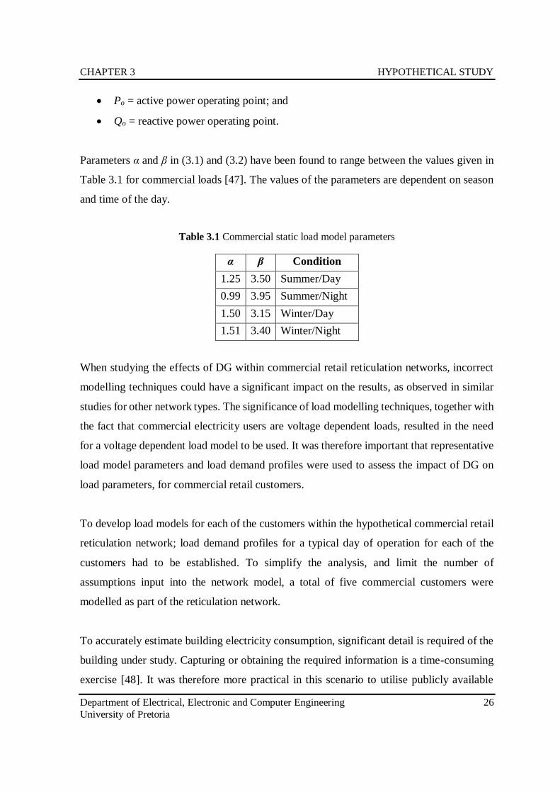
Parameters α and β in (3.1) and (3.2) have been found to range between the values given in
Table 3.1 for commercial loads [47]. The values of the parameters are dependent on season
and time of the day.
Table 3.1 Commercial static load model parameters
α β Condition 1.25 3.50 Summer/Day
0.99 3.95 Summer/Night
1.50 3.15 Winter/Day
1.51 3.40 Winter/Night
When studying the effects of DG within commercial retail reticulation networks, incorrect
modelling techniques could have a significant impact on the results, as observed in similar
studies for other network types. The significance of load modelling techniques, together with
the fact that commercial electricity users are voltage dependent loads, resulted in the need
for a voltage dependent load model to be used. It was therefore important that representative
load model parameters and load demand profiles were used to assess the impact of DG on
load parameters, for commercial retail customers.
To develop load models for each of the customers within the hypothetical commercial retail
reticulation network; load demand profiles for a typical day of operation for each of the
customers had to be established. To simplify the analysis, and limit the number of
assumptions input into the network model, a total of five commercial customers were
modelled as part of the reticulation network.
To accurately estimate building electricity consumption, significant detail is required of the
building under study. Capturing or obtaining the required information is a time-consuming
exercise [48]. It was therefore more practical in this scenario to utilise publicly available
CHAPTER 3 HYPOTHETICAL STUDY
Department of Electrical, Electronic and Computer Engineering 27
University of Pretoria
data for commercial retail building’s load consumption and demand profiles to develop
typical load models for this study [49], [50]. Unfortunately, all publicly available sources
are of commercial retail facilities based in the United States of America (USA). Differences
are expected between commercial retail load demands taken for facilities in the USA, when
compared to commercial retail facilities in South Africa. This would be due to the difference
in building material used in the two countries as well as the fact that the USA is a developed
country and South Africa is still a developing country. Due to the lack of publicly available
measured load data for commercial retail customers within South Africa, utilising
commercial retail load demand data from facilities in the USA was the best alternative to
basing simulated load demand profiles on purely assumed load demand profiles, resulting in
more reliable results for the hypothetical study. These results could be compared to the case
study results (Chapter 4), which are based on a commercial retail facility in South Africa.
Based on the two commercial building load demand databases available [49], [50] it was
found that only one database [50] was best suited for developing a normalised load demand
profile, as this source contained an hourly load schedule. A typical weekday hourly load
demand profile was developed by utilising hourly load schedule information. The data was
normalised to obtain a per unit or normalised load demand profile, as seen in Figure 3.1 The
normalised load demand profile was then scaled accordingly to obtain the expected load
demand profile for each customer. Each customer’s load demand profile was based on the
normalised load demand profile given in Figure 3.1, with each being slightly altered. The
load demand profiles were altered such that the maximum coincident demand of each
customer did not occur at the same hour of the day, and were also of different magnitudes.
This was done to introduce variability into the study and all modifications were based on
what would be expected in a real-life scenario.
In addition to introducing variations into the study by implementing differing load demand
profiles, different maximum load demands for each of the customers was assumed. Two
different maximum load demands were selected; one to represent a mid-size commercial
retail customer and a second to represent a larger sized commercial retail customer. The
maximum load demand for each type of commercial retail customer was based on 75% of
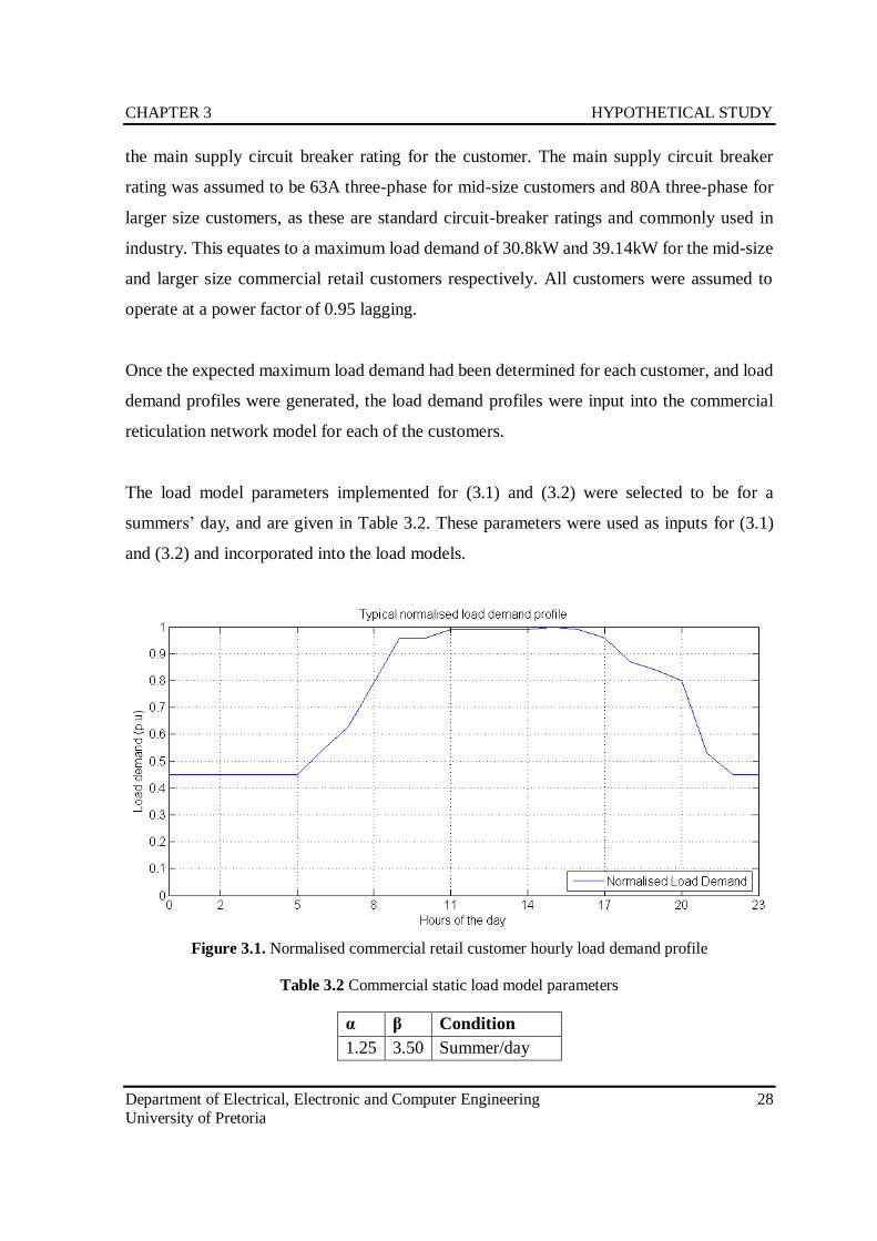
CHAPTER 3 HYPOTHETICAL STUDY
Department of Electrical, Electronic and Computer Engineering 28
University of Pretoria
the main supply circuit breaker rating for the customer. The main supply circuit breaker
rating was assumed to be 63A three-phase for mid-size customers and 80A three-phase for
larger size customers, as these are standard circuit-breaker ratings and commonly used in
industry. This equates to a maximum load demand of 30.8kW and 39.14kW for the mid-size
and larger size commercial retail customers respectively. All customers were assumed to
operate at a power factor of 0.95 lagging.
Once the expected maximum load demand had been determined for each customer, and load
demand profiles were generated, the load demand profiles were input into the commercial
reticulation network model for each of the customers.
The load model parameters implemented for (3.1) and (3.2) were selected to be for a
summers’ day, and are given in Table 3.2. These parameters were used as inputs for (3.1)
and (3.2) and incorporated into the load models.
Figure 3.1. Normalised commercial retail customer hourly load demand profile
Table 3.2 Commercial static load model parameters
α β Condition
1.25 3.50 Summer/day
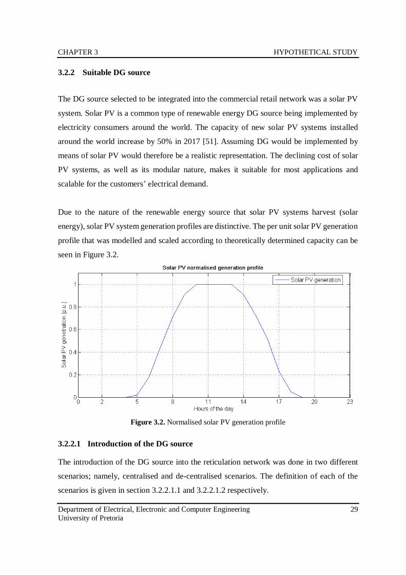
CHAPTER 3 HYPOTHETICAL STUDY
Department of Electrical, Electronic and Computer Engineering 29
University of Pretoria
3.2.2 Suitable DG source
The DG source selected to be integrated into the commercial retail network was a solar PV
system. Solar PV is a common type of renewable energy DG source being implemented by
electricity consumers around the world. The capacity of new solar PV systems installed
around the world increase by 50% in 2017 [51]. Assuming DG would be implemented by
means of solar PV would therefore be a realistic representation. The declining cost of solar
PV systems, as well as its modular nature, makes it suitable for most applications and
scalable for the customers’ electrical demand.
Due to the nature of the renewable energy source that solar PV systems harvest (solar
energy), solar PV system generation profiles are distinctive. The per unit solar PV generation
profile that was modelled and scaled according to theoretically determined capacity can be
seen in Figure 3.2.
Figure 3.2. Normalised solar PV generation profile
3.2.2.1 Introduction of the DG source
The introduction of the DG source into the reticulation network was done in two different
scenarios; namely, centralised and de-centralised scenarios. The definition of each of the
scenarios is given in section 3.2.2.1.1 and 3.2.2.1.2 respectively.
CHAPTER 3 HYPOTHETICAL STUDY
Department of Electrical, Electronic and Computer Engineering 30
University of Pretoria
3.2.2.1.1 Centralised DG scenario
In the centralised DG scenario a DG source was introduced into the reticulation network at
the main low-voltage supply point to the commercial retail reticulation network. The DG
source capacity was varied, from zero to the maximum coincident load demand at the busbar
it was connected to. This was done to understand the effect of DG and penetration levels on
the various load and network parameters under investigation.
3.2.2.1.2 De-centralised DG scenario
The second scenario (de-central DG) was to introduce the DG source further downstream
within the reticulation network and to vary the penetration level based on the maximum load
demand of the respective customer to which it was connected.
3.2.3 Reticulation network model
Once the load modelling was complete, the next step was to develop a reticulation network
model to conduct the required analysis and obtain results. To analyse the impact of varying
load demand over a specific period and DG output, quasi-dynamic load flow simulation
studies were conducted. The studies were conducted over a 24-hour period.
3.2.3.1 Network topology
A number of studies have implemented standard Institute of Electrical and Electronic
Engineers (IEEE) test networks to conduct the required analyses [42], [52]-[54] to determine
the effect of DG on a number of network parameters. These test networks are mainly
transmission and distribution systems which are high-voltage systems. They are therefore
not representative of commercial retail reticulation networks, as a commercial retail
reticulation network is typically a low-voltage network. There are also standard low-voltage
network test systems available [55]; however, these low-voltage reticulation test networks
contain several hundred nodes. These are therefore more representative of larger scale
reticulation networks rather than a network containing five customers. The test networks are
therefore not representative of a commercial retail reticulation network, as it is expected that
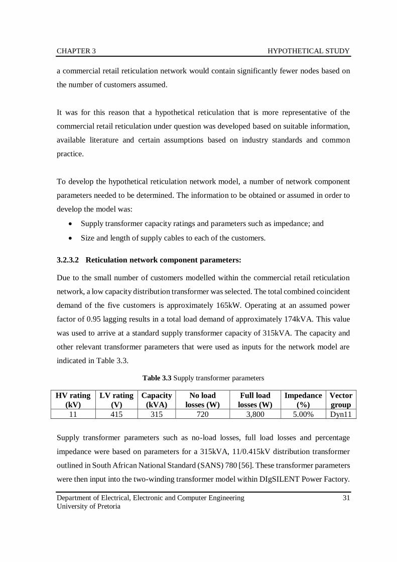
CHAPTER 3 HYPOTHETICAL STUDY
Department of Electrical, Electronic and Computer Engineering 31
University of Pretoria
a commercial retail reticulation network would contain significantly fewer nodes based on
the number of customers assumed.
It was for this reason that a hypothetical reticulation that is more representative of the
commercial retail reticulation under question was developed based on suitable information,
available literature and certain assumptions based on industry standards and common
practice.
To develop the hypothetical reticulation network model, a number of network component
parameters needed to be determined. The information to be obtained or assumed in order to
develop the model was:
• Supply transformer capacity ratings and parameters such as impedance; and
• Size and length of supply cables to each of the customers.
3.2.3.2 Reticulation network component parameters:
Due to the small number of customers modelled within the commercial retail reticulation
network, a low capacity distribution transformer was selected. The total combined coincident
demand of the five customers is approximately 165kW. Operating at an assumed power
factor of 0.95 lagging results in a total load demand of approximately 174kVA. This value
was used to arrive at a standard supply transformer capacity of 315kVA. The capacity and
other relevant transformer parameters that were used as inputs for the network model are
indicated in Table 3.3.
Table 3.3 Supply transformer parameters
HV rating
(kV)
LV rating
(V)
Capacity
(kVA)
No load
losses (W)
Full load
losses (W)
Impedance
(%)
Vector
group
11 415 315 720 3,800 5.00% Dyn11
Supply transformer parameters such as no-load losses, full load losses and percentage
impedance were based on parameters for a 315kVA, 11/0.415kV distribution transformer
outlined in South African National Standard (SANS) 780 [56]. These transformer parameters
were then input into the two-winding transformer model within DIgSILENT Power Factory.
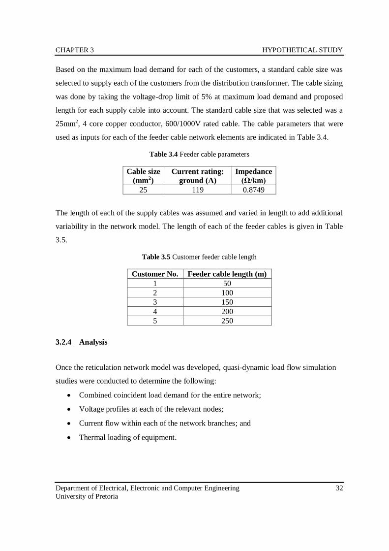
CHAPTER 3 HYPOTHETICAL STUDY
Department of Electrical, Electronic and Computer Engineering 32
University of Pretoria
Based on the maximum load demand for each of the customers, a standard cable size was
selected to supply each of the customers from the distribution transformer. The cable sizing
was done by taking the voltage-drop limit of 5% at maximum load demand and proposed
length for each supply cable into account. The standard cable size that was selected was a
25mm2, 4 core copper conductor, 600/1000V rated cable. The cable parameters that were
used as inputs for each of the feeder cable network elements are indicated in Table 3.4.
Table 3.4 Feeder cable parameters
Cable size
(mm2)
Current rating:
ground (A)
Impedance
(Ω/km)
25 119 0.8749
The length of each of the supply cables was assumed and varied in length to add additional
variability in the network model. The length of each of the feeder cables is given in Table
3.5.
Table 3.5 Customer feeder cable length
Customer No. Feeder cable length (m)
1 50
2 100
3 150
4 200
5 250
3.2.4 Analysis
Once the reticulation network model was developed, quasi-dynamic load flow simulation
studies were conducted to determine the following:
• Combined coincident load demand for the entire network;
• Voltage profiles at each of the relevant nodes;
• Current flow within each of the network branches; and
• Thermal loading of equipment.
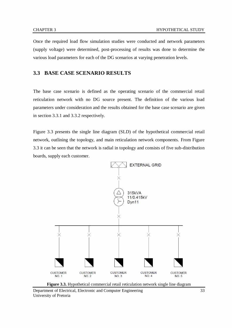
CHAPTER 3 HYPOTHETICAL STUDY
Department of Electrical, Electronic and Computer Engineering 33
University of Pretoria
Once the required load flow simulation studies were conducted and network parameters
(supply voltage) were determined, post-processing of results was done to determine the
various load parameters for each of the DG scenarios at varying penetration levels.
3.3 BASE CASE SCENARIO RESULTS
The base case scenario is defined as the operating scenario of the commercial retail
reticulation network with no DG source present. The definition of the various load
parameters under consideration and the results obtained for the base case scenario are given
in section 3.3.1 and 3.3.2 respectively.
Figure 3.3 presents the single line diagram (SLD) of the hypothetical commercial retail
network, outlining the topology, and main reticulation network components. From Figure
3.3 it can be seen that the network is radial in topology and consists of five sub-distribution
boards, supply each customer.
Figure 3.3. Hypothetical commercial retail reticulation network single line diagram
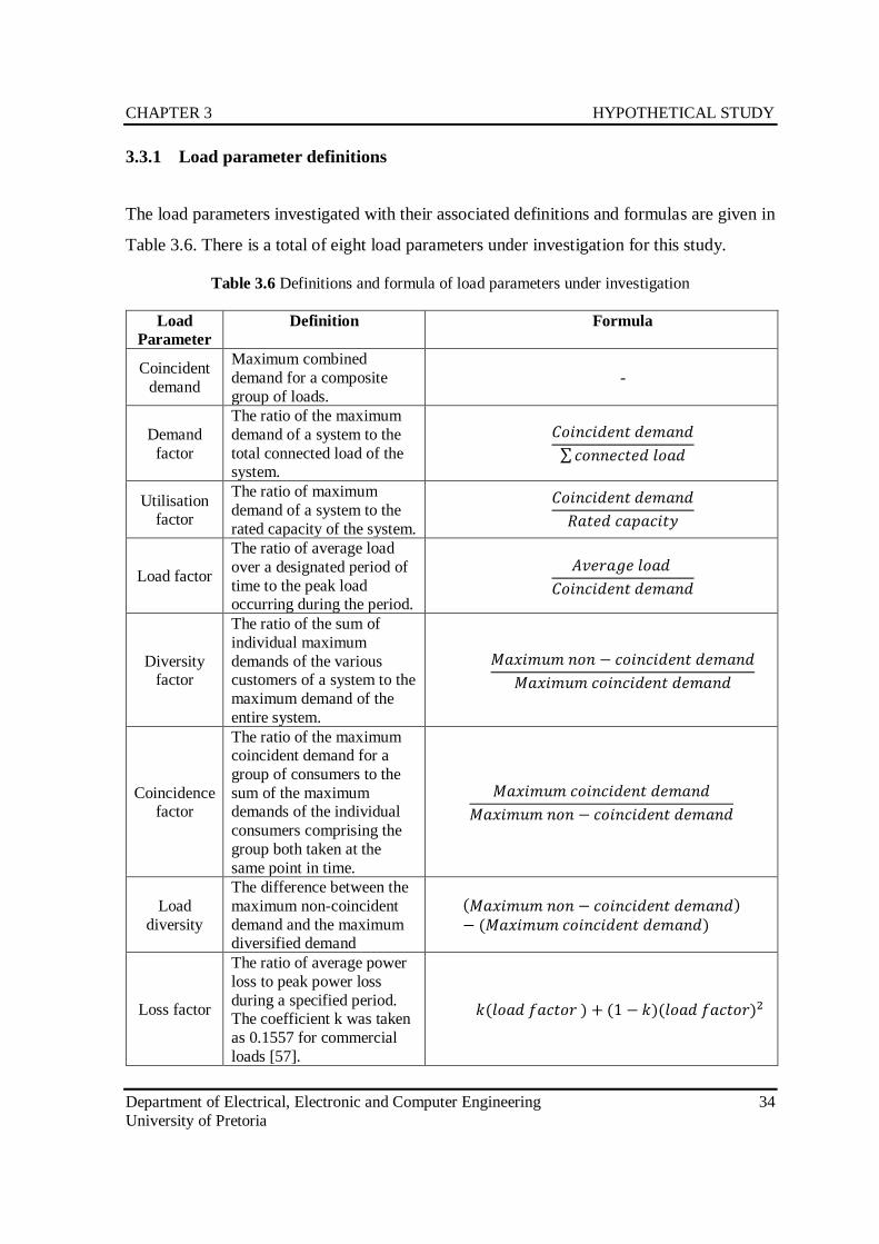
CHAPTER 3 HYPOTHETICAL STUDY
Department of Electrical, Electronic and Computer Engineering 34
University of Pretoria
3.3.1 Load parameter definitions
The load parameters investigated with their associated definitions and formulas are given in
Table 3.6. There is a total of eight load parameters under investigation for this study.
Table 3.6 Definitions and formula of load parameters under investigation
Load
Parameter
Definition Formula
Coincident
demand
Maximum combined
demand for a composite
group of loads.
-
Demand
factor
The ratio of the maximum
demand of a system to the
total connected load of the system.
𝐶𝑜𝑖𝑛𝑐𝑖𝑑𝑒𝑛𝑡 𝑑𝑒𝑚𝑎𝑛𝑑
∑ 𝑐𝑜𝑛𝑛𝑒𝑐𝑡𝑒𝑑 𝑙𝑜𝑎𝑑
Utilisation factor
The ratio of maximum
demand of a system to the
rated capacity of the system.
𝐶𝑜𝑖𝑛𝑐𝑖𝑑𝑒𝑛𝑡 𝑑𝑒𝑚𝑎𝑛𝑑
𝑅𝑎𝑡𝑒𝑑 𝑐𝑎𝑝𝑎𝑐𝑖𝑡𝑦
Load factor
The ratio of average load
over a designated period of
time to the peak load occurring during the period.
𝐴𝑣𝑒𝑟𝑎𝑔𝑒 𝑙𝑜𝑎𝑑
𝐶𝑜𝑖𝑛𝑐𝑖𝑑𝑒𝑛𝑡 𝑑𝑒𝑚𝑎𝑛𝑑
Diversity factor
The ratio of the sum of
individual maximum
demands of the various customers of a system to the
maximum demand of the
entire system.
𝑀𝑎𝑥𝑖𝑚𝑢𝑚 𝑛𝑜𝑛 − 𝑐𝑜𝑖𝑛𝑐𝑖𝑑𝑒𝑛𝑡 𝑑𝑒𝑚𝑎𝑛𝑑
𝑀𝑎𝑥𝑖𝑚𝑢𝑚 𝑐𝑜𝑖𝑛𝑐𝑖𝑑𝑒𝑛𝑡 𝑑𝑒𝑚𝑎𝑛𝑑
Coincidence factor
The ratio of the maximum coincident demand for a
group of consumers to the
sum of the maximum demands of the individual
consumers comprising the
group both taken at the
same point in time.
𝑀𝑎𝑥𝑖𝑚𝑢𝑚 𝑐𝑜𝑖𝑛𝑐𝑖𝑑𝑒𝑛𝑡 𝑑𝑒𝑚𝑎𝑛𝑑
𝑀𝑎𝑥𝑖𝑚𝑢𝑚 𝑛𝑜𝑛 − 𝑐𝑜𝑖𝑛𝑐𝑖𝑑𝑒𝑛𝑡 𝑑𝑒𝑚𝑎𝑛𝑑
Load
diversity
The difference between the
maximum non-coincident
demand and the maximum diversified demand
(𝑀𝑎𝑥𝑖𝑚𝑢𝑚 𝑛𝑜𝑛 − 𝑐𝑜𝑖𝑛𝑐𝑖𝑑𝑒𝑛𝑡 𝑑𝑒𝑚𝑎𝑛𝑑)− (𝑀𝑎𝑥𝑖𝑚𝑢𝑚 𝑐𝑜𝑖𝑛𝑐𝑖𝑑𝑒𝑛𝑡 𝑑𝑒𝑚𝑎𝑛𝑑)
Loss factor
The ratio of average power
loss to peak power loss
during a specified period. The coefficient k was taken
as 0.1557 for commercial
loads [57].
𝑘(𝑙𝑜𝑎𝑑 𝑓𝑎𝑐𝑡𝑜𝑟 ) + (1 − 𝑘)(𝑙𝑜𝑎𝑑 𝑓𝑎𝑐𝑡𝑜𝑟)2
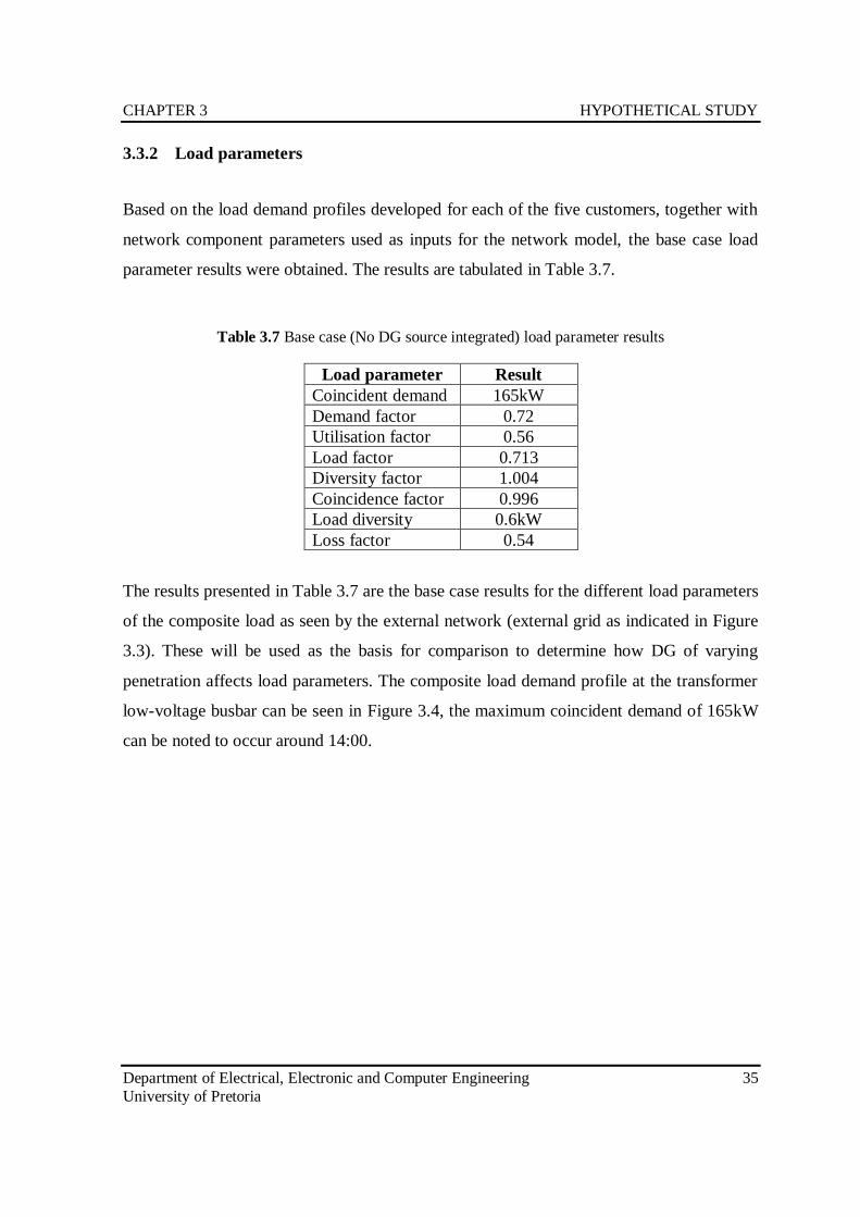
CHAPTER 3 HYPOTHETICAL STUDY
Department of Electrical, Electronic and Computer Engineering 35
University of Pretoria
3.3.2 Load parameters
Based on the load demand profiles developed for each of the five customers, together with
network component parameters used as inputs for the network model, the base case load
parameter results were obtained. The results are tabulated in Table 3.7.
Table 3.7 Base case (No DG source integrated) load parameter results
Load parameter Result
Coincident demand 165kW
Demand factor 0.72
Utilisation factor 0.56
Load factor 0.713
Diversity factor 1.004
Coincidence factor 0.996
Load diversity 0.6kW
Loss factor 0.54
The results presented in Table 3.7 are the base case results for the different load parameters
of the composite load as seen by the external network (external grid as indicated in Figure
3.3). These will be used as the basis for comparison to determine how DG of varying
penetration affects load parameters. The composite load demand profile at the transformer
low-voltage busbar can be seen in Figure 3.4, the maximum coincident demand of 165kW
can be noted to occur around 14:00.
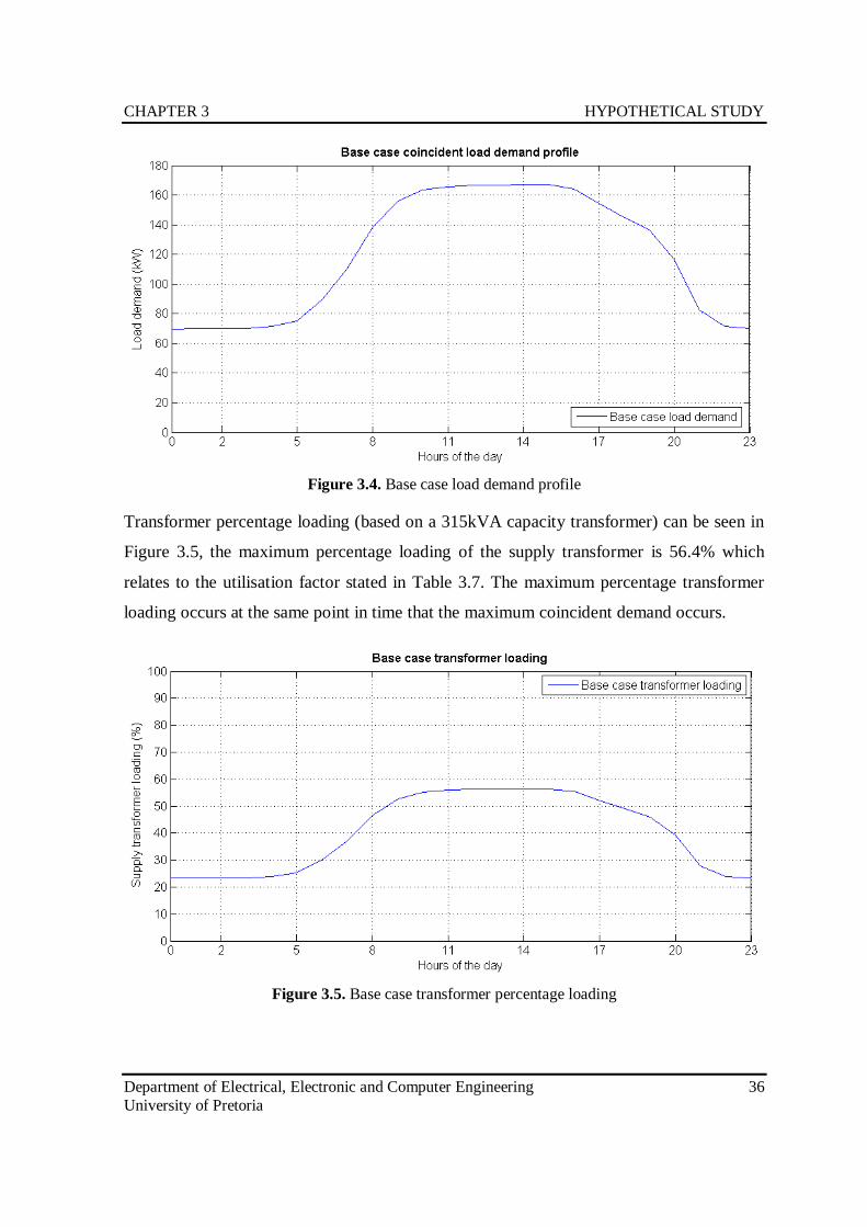
CHAPTER 3 HYPOTHETICAL STUDY
Department of Electrical, Electronic and Computer Engineering 36
University of Pretoria
Figure 3.4. Base case load demand profile
Transformer percentage loading (based on a 315kVA capacity transformer) can be seen in
Figure 3.5, the maximum percentage loading of the supply transformer is 56.4% which
relates to the utilisation factor stated in Table 3.7. The maximum percentage transformer
loading occurs at the same point in time that the maximum coincident demand occurs.
Figure 3.5. Base case transformer percentage loading
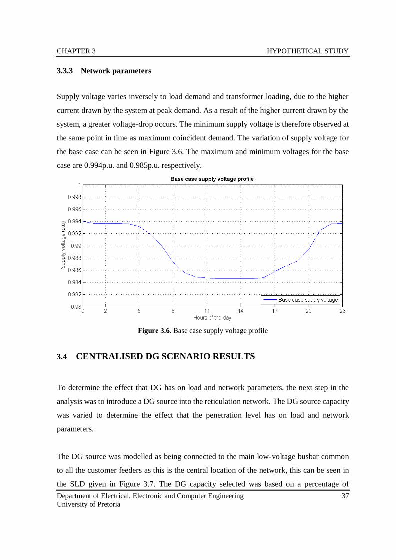
CHAPTER 3 HYPOTHETICAL STUDY
Department of Electrical, Electronic and Computer Engineering 37
University of Pretoria
3.3.3 Network parameters
Supply voltage varies inversely to load demand and transformer loading, due to the higher
current drawn by the system at peak demand. As a result of the higher current drawn by the
system, a greater voltage-drop occurs. The minimum supply voltage is therefore observed at
the same point in time as maximum coincident demand. The variation of supply voltage for
the base case can be seen in Figure 3.6. The maximum and minimum voltages for the base
case are 0.994p.u. and 0.985p.u. respectively.
Figure 3.6. Base case supply voltage profile
3.4 CENTRALISED DG SCENARIO RESULTS
To determine the effect that DG has on load and network parameters, the next step in the
analysis was to introduce a DG source into the reticulation network. The DG source capacity
was varied to determine the effect that the penetration level has on load and network
parameters.
The DG source was modelled as being connected to the main low-voltage busbar common
to all the customer feeders as this is the central location of the network, this can be seen in
the SLD given in Figure 3.7. The DG capacity selected was based on a percentage of

CHAPTER 3 HYPOTHETICAL STUDY
Department of Electrical, Electronic and Computer Engineering 38
University of Pretoria
maximum load demand as obtained in the base case results (167kW). The DG penetration
levels investigated are indicated in Table 3.8.
Figure 3.7. Single line diagram with central DG source
Table 3.8 Solar PV penetration levels and capacities modelled
Percentage
penetration
Solar PV
capacity (kWac)
10% 16.50
15% 24.75
20% 33.00
25% 41.25
50% 82.50
75% 123.75
100% 165.00
It should be noted that the capacities of the solar PV system modelled within the reticulation
network are theoretical capacities only, and are not all practically achievable. This is due to
solar PV system components, such as inverters, only being manufactured in discrete sizes.
Although not practically achievable, these theoretical capacities assisted in gaining valuable
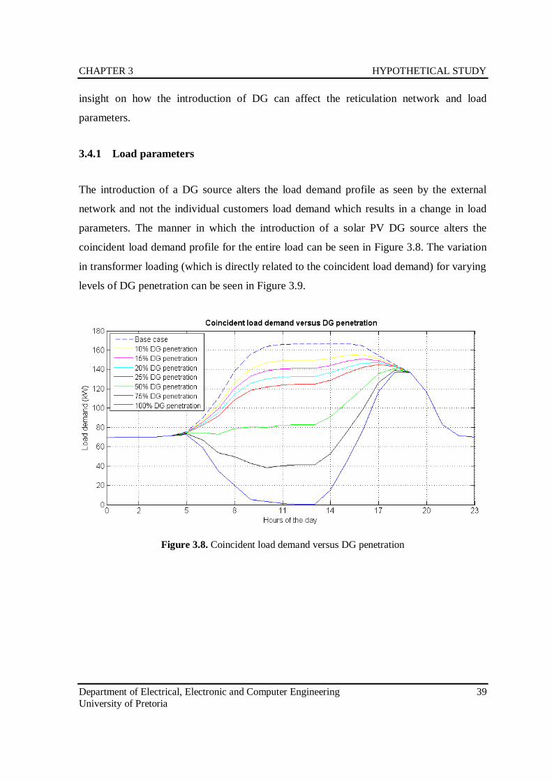
CHAPTER 3 HYPOTHETICAL STUDY
Department of Electrical, Electronic and Computer Engineering 39
University of Pretoria
insight on how the introduction of DG can affect the reticulation network and load
parameters.
3.4.1 Load parameters
The introduction of a DG source alters the load demand profile as seen by the external
network and not the individual customers load demand which results in a change in load
parameters. The manner in which the introduction of a solar PV DG source alters the
coincident load demand profile for the entire load can be seen in Figure 3.8. The variation
in transformer loading (which is directly related to the coincident load demand) for varying
levels of DG penetration can be seen in Figure 3.9.
Figure 3.8. Coincident load demand versus DG penetration
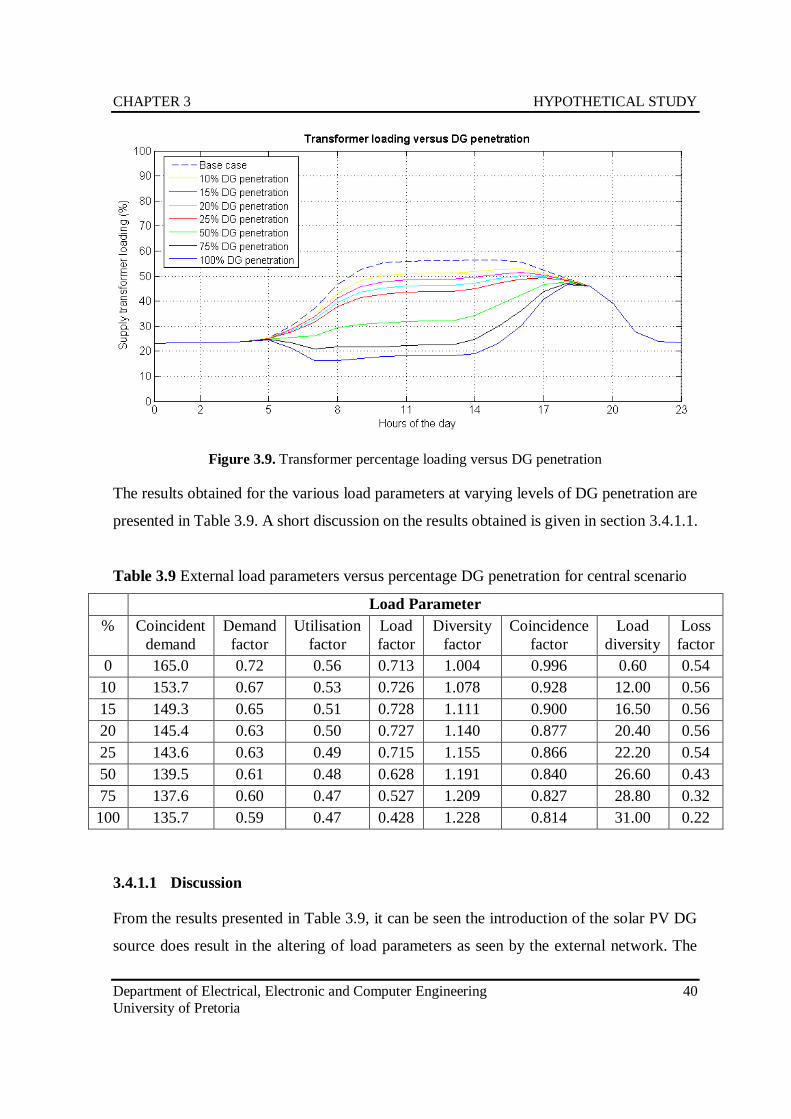
CHAPTER 3 HYPOTHETICAL STUDY
Department of Electrical, Electronic and Computer Engineering 40
University of Pretoria
Figure 3.9. Transformer percentage loading versus DG penetration
The results obtained for the various load parameters at varying levels of DG penetration are
presented in Table 3.9. A short discussion on the results obtained is given in section 3.4.1.1.
Table 3.9 External load parameters versus percentage DG penetration for central scenario
Load Parameter
% Coincident
demand
Demand
factor
Utilisation
factor
Load
factor
Diversity
factor
Coincidence
factor
Load
diversity
Loss
factor
0 165.0 0.72 0.56 0.713 1.004 0.996 0.60 0.54
10 153.7 0.67 0.53 0.726 1.078 0.928 12.00 0.56
15 149.3 0.65 0.51 0.728 1.111 0.900 16.50 0.56
20 145.4 0.63 0.50 0.727 1.140 0.877 20.40 0.56
25 143.6 0.63 0.49 0.715 1.155 0.866 22.20 0.54
50 139.5 0.61 0.48 0.628 1.191 0.840 26.60 0.43
75 137.6 0.60 0.47 0.527 1.209 0.827 28.80 0.32
100 135.7 0.59 0.47 0.428 1.228 0.814 31.00 0.22
3.4.1.1 Discussion
From the results presented in Table 3.9, it can be seen the introduction of the solar PV DG
source does result in the altering of load parameters as seen by the external network. The
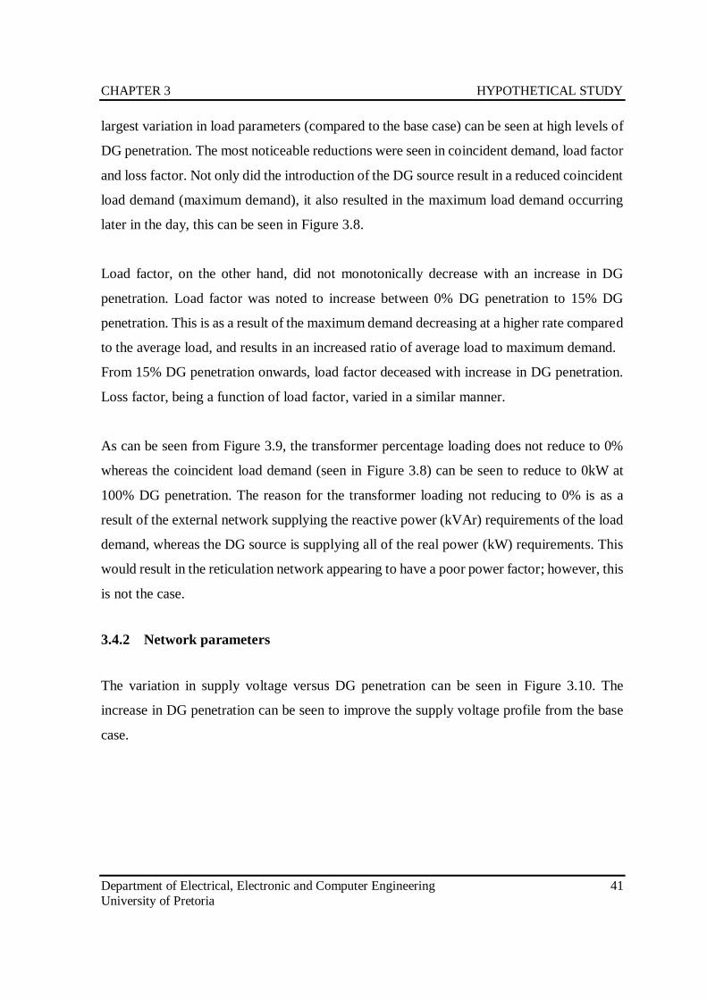
CHAPTER 3 HYPOTHETICAL STUDY
Department of Electrical, Electronic and Computer Engineering 41
University of Pretoria
largest variation in load parameters (compared to the base case) can be seen at high levels of
DG penetration. The most noticeable reductions were seen in coincident demand, load factor
and loss factor. Not only did the introduction of the DG source result in a reduced coincident
load demand (maximum demand), it also resulted in the maximum load demand occurring
later in the day, this can be seen in Figure 3.8.
Load factor, on the other hand, did not monotonically decrease with an increase in DG
penetration. Load factor was noted to increase between 0% DG penetration to 15% DG
penetration. This is as a result of the maximum demand decreasing at a higher rate compared
to the average load, and results in an increased ratio of average load to maximum demand.
From 15% DG penetration onwards, load factor deceased with increase in DG penetration.
Loss factor, being a function of load factor, varied in a similar manner.
As can be seen from Figure 3.9, the transformer percentage loading does not reduce to 0%
whereas the coincident load demand (seen in Figure 3.8) can be seen to reduce to 0kW at
100% DG penetration. The reason for the transformer loading not reducing to 0% is as a
result of the external network supplying the reactive power (kVAr) requirements of the load
demand, whereas the DG source is supplying all of the real power (kW) requirements. This
would result in the reticulation network appearing to have a poor power factor; however, this
is not the case.
3.4.2 Network parameters
The variation in supply voltage versus DG penetration can be seen in Figure 3.10. The
increase in DG penetration can be seen to improve the supply voltage profile from the base
case.
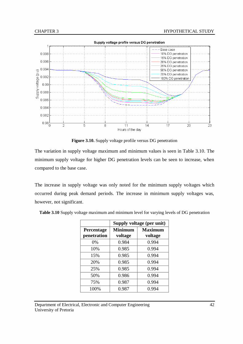
CHAPTER 3 HYPOTHETICAL STUDY
Department of Electrical, Electronic and Computer Engineering 42
University of Pretoria
Figure 3.10. Supply voltage profile versus DG penetration
The variation in supply voltage maximum and minimum values is seen in Table 3.10. The
minimum supply voltage for higher DG penetration levels can be seen to increase, when
compared to the base case.
The increase in supply voltage was only noted for the minimum supply voltages which
occurred during peak demand periods. The increase in minimum supply voltages was,
however, not significant.
Table 3.10 Supply voltage maximum and minimum level for varying levels of DG penetration
Supply voltage (per unit)
Percentage
penetration
Minimum
voltage
Maximum
voltage
0% 0.984 0.994
10% 0.985 0.994
15% 0.985 0.994
20% 0.985 0.994
25% 0.985 0.994
50% 0.986 0.994
75% 0.987 0.994
100% 0.987 0.994
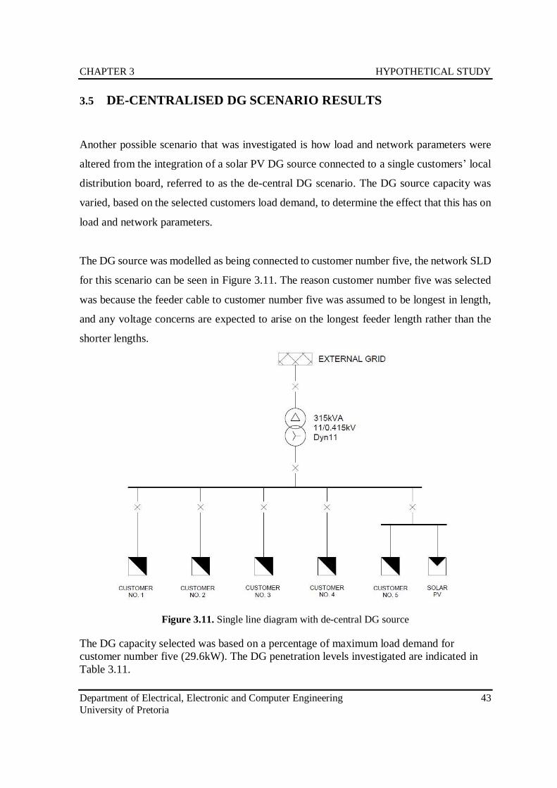
CHAPTER 3 HYPOTHETICAL STUDY
Department of Electrical, Electronic and Computer Engineering 43
University of Pretoria
3.5 DE-CENTRALISED DG SCENARIO RESULTS
Another possible scenario that was investigated is how load and network parameters were
altered from the integration of a solar PV DG source connected to a single customers’ local
distribution board, referred to as the de-central DG scenario. The DG source capacity was
varied, based on the selected customers load demand, to determine the effect that this has on
load and network parameters.
The DG source was modelled as being connected to customer number five, the network SLD
for this scenario can be seen in Figure 3.11. The reason customer number five was selected
was because the feeder cable to customer number five was assumed to be longest in length,
and any voltage concerns are expected to arise on the longest feeder length rather than the
shorter lengths.
Figure 3.11. Single line diagram with de-central DG source
The DG capacity selected was based on a percentage of maximum load demand for
customer number five (29.6kW). The DG penetration levels investigated are indicated in
Table 3.11.
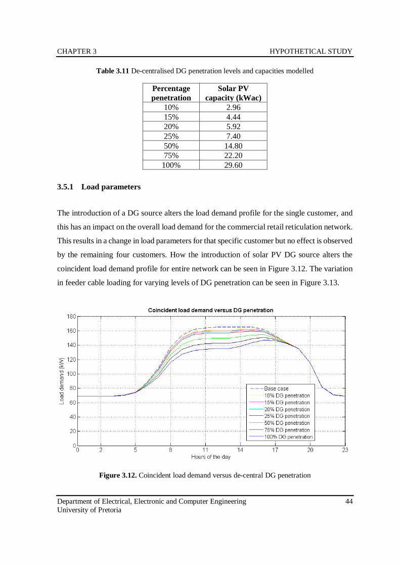
CHAPTER 3 HYPOTHETICAL STUDY
Department of Electrical, Electronic and Computer Engineering 44
University of Pretoria
Table 3.11 De-centralised DG penetration levels and capacities modelled
Percentage
penetration
Solar PV
capacity (kWac)
10% 2.96
15% 4.44
20% 5.92
25% 7.40
50% 14.80
75% 22.20
100% 29.60
3.5.1 Load parameters
The introduction of a DG source alters the load demand profile for the single customer, and
this has an impact on the overall load demand for the commercial retail reticulation network.
This results in a change in load parameters for that specific customer but no effect is observed
by the remaining four customers. How the introduction of solar PV DG source alters the
coincident load demand profile for entire network can be seen in Figure 3.12. The variation
in feeder cable loading for varying levels of DG penetration can be seen in Figure 3.13.
Figure 3.12. Coincident load demand versus de-central DG penetration
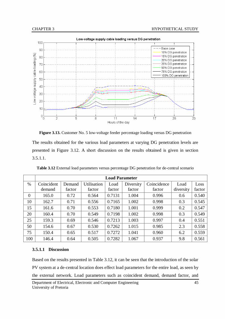
CHAPTER 3 HYPOTHETICAL STUDY
Department of Electrical, Electronic and Computer Engineering 45
University of Pretoria
Figure 3.13. Customer No. 5 low-voltage feeder percentage loading versus DG penetration
The results obtained for the various load parameters at varying DG penetration levels are
presented in Figure 3.12. A short discussion on the results obtained is given in section
3.5.1.1.
Table 3.12 External load parameters versus percentage DG penetration for de-central scenario
Load Parameter
% Coincident
demand
Demand
factor
Utilisation
factor
Load
factor
Diversity
factor
Coincidence
factor
Load
diversity
Loss
factor
0 165.0 0.72 0.564 0.7131 1.004 0.996 0.6 0.540
10 162.7 0.71 0.556 0.7165 1.002 0.998 0.3 0.545
15 161.6 0.70 0.553 0.7180 1.001 0.999 0.2 0.547
20 160.4 0.70 0.549 0.7198 1.002 0.998 0.3 0.549
25 159.3 0.69 0.546 0.7213 1.003 0.997 0.4 0.551
50 154.6 0.67 0.530 0.7262 1.015 0.985 2.3 0.558
75 150.4 0.65 0.517 0.7272 1.041 0.960 6.2 0.559
100 146.4 0.64 0.505 0.7282 1.067 0.937 9.8 0.561
3.5.1.1 Discussion
Based on the results presented in Table 3.12, it can be seen that the introduction of the solar
PV system at a de-central location does effect load parameters for the entire load, as seen by
the external network. Load parameters such as coincident demand, demand factor, and
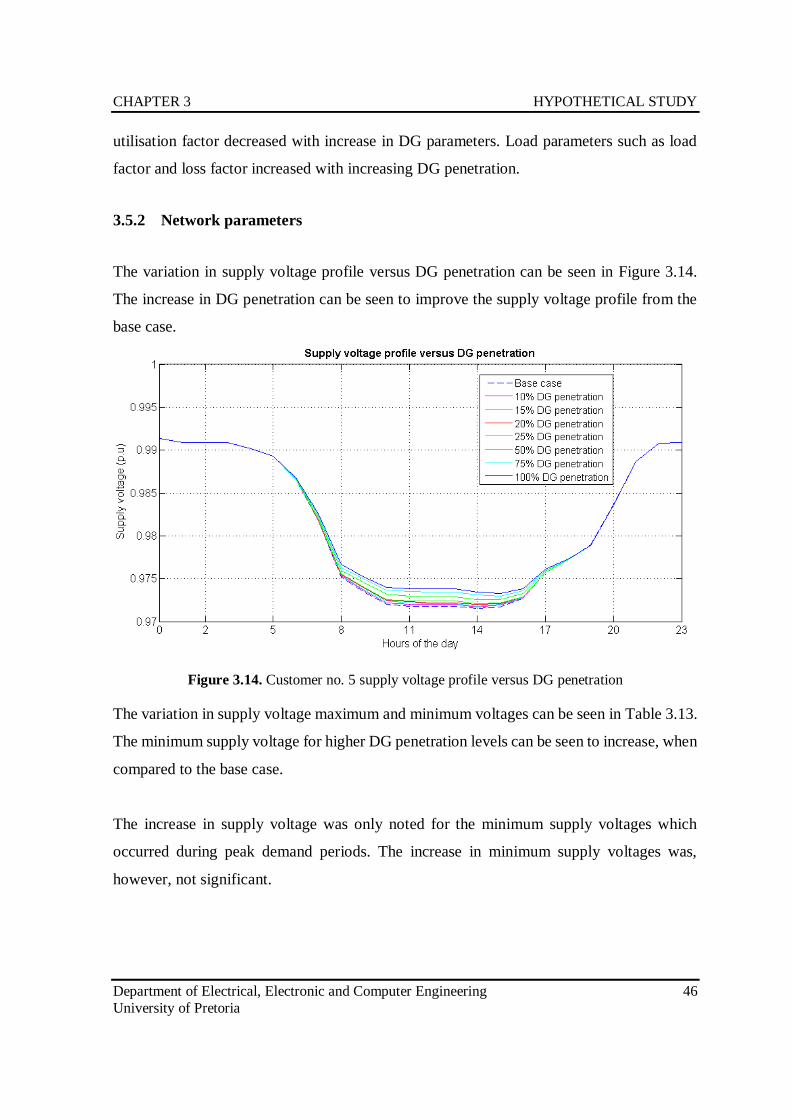
CHAPTER 3 HYPOTHETICAL STUDY
Department of Electrical, Electronic and Computer Engineering 46
University of Pretoria
utilisation factor decreased with increase in DG parameters. Load parameters such as load
factor and loss factor increased with increasing DG penetration.
3.5.2 Network parameters
The variation in supply voltage profile versus DG penetration can be seen in Figure 3.14.
The increase in DG penetration can be seen to improve the supply voltage profile from the
base case.
Figure 3.14. Customer no. 5 supply voltage profile versus DG penetration
The variation in supply voltage maximum and minimum voltages can be seen in Table 3.13.
The minimum supply voltage for higher DG penetration levels can be seen to increase, when
compared to the base case.
The increase in supply voltage was only noted for the minimum supply voltages which
occurred during peak demand periods. The increase in minimum supply voltages was,
however, not significant.
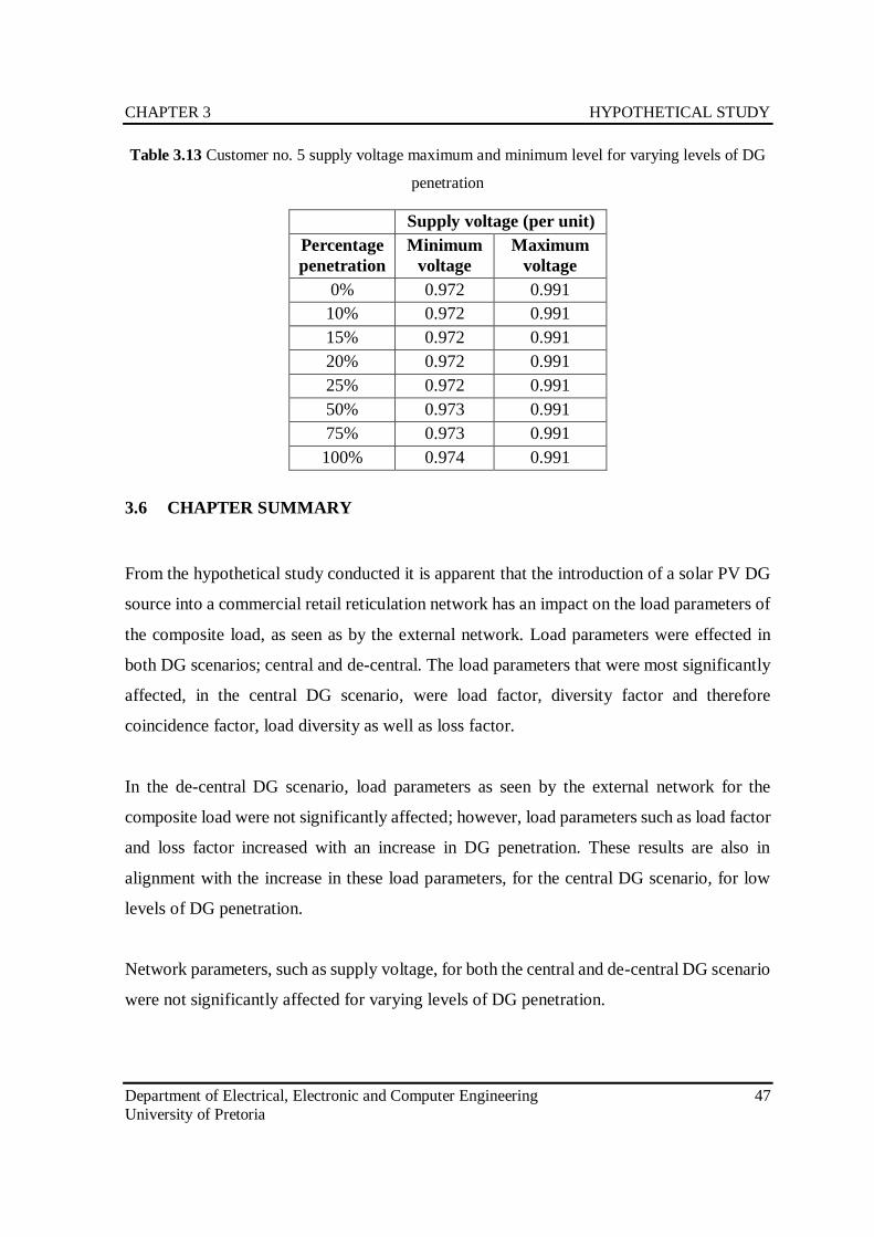
CHAPTER 3 HYPOTHETICAL STUDY
Department of Electrical, Electronic and Computer Engineering 47
University of Pretoria
Table 3.13 Customer no. 5 supply voltage maximum and minimum level for varying levels of DG
penetration
Supply voltage (per unit)
Percentage
penetration
Minimum
voltage
Maximum
voltage
0% 0.972 0.991
10% 0.972 0.991
15% 0.972 0.991
20% 0.972 0.991
25% 0.972 0.991
50% 0.973 0.991
75% 0.973 0.991
100% 0.974 0.991
3.6 CHAPTER SUMMARY
From the hypothetical study conducted it is apparent that the introduction of a solar PV DG
source into a commercial retail reticulation network has an impact on the load parameters of
the composite load, as seen as by the external network. Load parameters were effected in
both DG scenarios; central and de-central. The load parameters that were most significantly
affected, in the central DG scenario, were load factor, diversity factor and therefore
coincidence factor, load diversity as well as loss factor.
In the de-central DG scenario, load parameters as seen by the external network for the
composite load were not significantly affected; however, load parameters such as load factor
and loss factor increased with an increase in DG penetration. These results are also in
alignment with the increase in these load parameters, for the central DG scenario, for low
levels of DG penetration.
Network parameters, such as supply voltage, for both the central and de-central DG scenario
were not significantly affected for varying levels of DG penetration.
CHAPTER 4 CASE STUDY
4.1 CHAPTER OVERVIEW
Chapter 4 presents the results obtained for the case study that was conducted to confirm the
results obtained for the hypothetical study. The case study was based on a network in service
with available load metered data. Section 4.2 provides detail on the information gathered
and input to develop the reticulation network model. Section 4.3 provides detail on the DG
source integrated into the reticulation network. Section 4.4 presents the base case results
obtained, where sections 4.5 and 4.6 presents the results for the centralised DG scenario and
de-centralised DG scenario respectively. Section 4.7 concludes the chapter.
4.2 METERED LOAD DATA AND EXISTING RETICULATION NETWORK
INFORMATION
A case study was completed to verify and validate the results obtained in chapter 3. The
study was based on an existing commercial retail park situated in Pretoria, South Africa. To
accurately develop a network model along with the load demands for each of the electricity
customers certain information was required. The information required was metered load
demand data for each of the customers within the reticulation network as well as equipment
ratings, capacities, size and configuration of the reticulation network in use. Section 4.2.1
and 4.2.2 provides further details on the information gathered to develop the network model
for the case study.
CHAPTER 4 CASE STUDY
Department of Electrical, Electronic and Computer Engineering 49
University of Pretoria
4.2.1 Load modelling
To develop representative load models for each of the customers within the commercial retail
reticulation network, recorded load demand information such as electricity demand, energy
consumption and power factor over time was required.
The measured load data obtained was analysed to determine an average half-hourly load
demand profile for each customer. This result was then used as the input to the load model
for the customer within the DIgSILENT network model. In addition to the average load
demand profile for each customer input to the DIgSILENT model, an average half-hourly
power factor profile over the same period of operation was also used as an input.
4.2.1.1 Load demand data
The existing commercial retail park consists of 40 separate office units; refer to Table 4.1
for a complete list of the individual units. Most of the units are individually metered, there
are however units for which there is no metered load demand data available. Metered load
demand data for each of the units, with energy meters installed, was download from an online
platform for the energy meters (Enermatics). Metering data downloaded was at a half-hourly
time interval. There are situations where there is metered data available for a unit; however,
the data was recorded as a zero value over the entire month. Metering data available covered
a single month at a time from 2016.
There is a single three-phase meter (incoming meter, labelled Garsfontein Office Park (GOP)
3 phase) that measures the total load demand of the commercial retail park, this metering
data was used as a check to determine if there are any errors in the data captured. It was
found that there was a discrepancy between the total measured load demand versus the sum
of each measured load demand per customer.
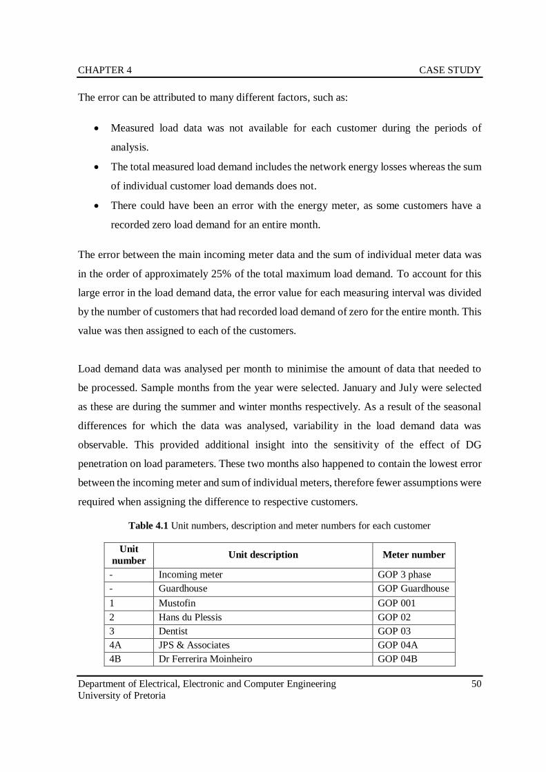
CHAPTER 4 CASE STUDY
Department of Electrical, Electronic and Computer Engineering 50
University of Pretoria
The error can be attributed to many different factors, such as:
• Measured load data was not available for each customer during the periods of
analysis.
• The total measured load demand includes the network energy losses whereas the sum
of individual customer load demands does not.
• There could have been an error with the energy meter, as some customers have a
recorded zero load demand for an entire month.
The error between the main incoming meter data and the sum of individual meter data was
in the order of approximately 25% of the total maximum load demand. To account for this
large error in the load demand data, the error value for each measuring interval was divided
by the number of customers that had recorded load demand of zero for the entire month. This
value was then assigned to each of the customers.
Load demand data was analysed per month to minimise the amount of data that needed to
be processed. Sample months from the year were selected. January and July were selected
as these are during the summer and winter months respectively. As a result of the seasonal
differences for which the data was analysed, variability in the load demand data was
observable. This provided additional insight into the sensitivity of the effect of DG
penetration on load parameters. These two months also happened to contain the lowest error
between the incoming meter and sum of individual meters, therefore fewer assumptions were
required when assigning the difference to respective customers.
Table 4.1 Unit numbers, description and meter numbers for each customer
Unit
number Unit description Meter number
- Incoming meter GOP 3 phase
- Guardhouse GOP Guardhouse
1 Mustofin GOP 001
2 Hans du Plessis GOP 02
3 Dentist GOP 03
4A JPS & Associates GOP 04A
4B Dr Ferrerira Moinheiro GOP 04B
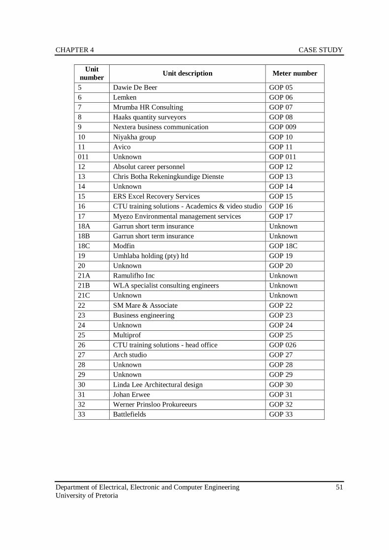
CHAPTER 4 CASE STUDY
Department of Electrical, Electronic and Computer Engineering 51
University of Pretoria
Unit
number Unit description Meter number
5 Dawie De Beer GOP 05
6 Lemken GOP 06
7 Mrumba HR Consulting GOP 07
8 Haaks quantity surveyors GOP 08
9 Nextera business communication GOP 009
10 Niyakha group GOP 10
11 Avico GOP 11
011 Unknown GOP 011
12 Absolut career personnel GOP 12
13 Chris Botha Rekeningkundige Dienste GOP 13
14 Unknown GOP 14
15 ERS Excel Recovery Services GOP 15
16 CTU training solutions - Academics & video studio GOP 16
17 Myezo Environmental management services GOP 17
18A Garrun short term insurance Unknown
18B Garrun short term insurance Unknown
18C Modfin GOP 18C
19 Umhlaba holding (pty) ltd GOP 19
20 Unknown GOP 20
21A Ramulifho Inc Unknown
21B WLA specialist consulting engineers Unknown
21C Unknown Unknown
22 SM Mare & Associate GOP 22
23 Business engineering GOP 23
24 Unknown GOP 24
25 Multiprof GOP 25
26 CTU training solutions - head office GOP 026
27 Arch studio GOP 27
28 Unknown GOP 28
29 Unknown GOP 29
30 Linda Lee Architectural design GOP 30
31 Johan Erwee GOP 31
32 Werner Prinsloo Prokureeurs GOP 32
33 Battlefields GOP 33
CHAPTER 4 CASE STUDY
Department of Electrical, Electronic and Computer Engineering 52
University of Pretoria
4.2.2 Reticulation network
The following information was obtained from an on-site inspection of the existing
reticulation network:
• Location of main and sub distribution boards;
• Location of step-down transformer supplying the network;
• Size of each of the feeder cables from the main distribution board to the sub
distribution boards;
• Network topology; and
• Circuit-breaker ratings of all incoming and outgoing circuit-breakers.
The above information was used to develop a network model for the reticulation network
using DIgSILENT Power Factory simulation software, as was done for the hypothetical
study. Not all of the required information to develop the network model was obtained from
the on-site inspection. Certain assumptions therefore needed to be made to develop the
network model, these assumptions were:
• Length of feeder cables; and
• Capacity and properties of the step-down transformer.
4.2.2.1 Length of feeder cables
The length of each of the feeder cables was determined using Google Earth by measuring
the distance between the main distribution board and sub distribution boards. Assumptions
with regards to the exact routing of the cables had to be made based on the facility layout,
which included parking area and roadway layout, layouts of walk-ways and locations of
distribution boards. The length of the main incoming feeder cable to the main distribution
board was also determined from Google Earth. Again, an assumption regarding the routing
of the cable had to be made. From the on-site inspection, the cable conductor cross-sectional
area and type of cable feeding the main distribution board was not clearly identified, and
therefore an additional assumption had to be made. The length, cable cross-sectional area
and type of all the cables within the reticulation network are given in Table 4.2.
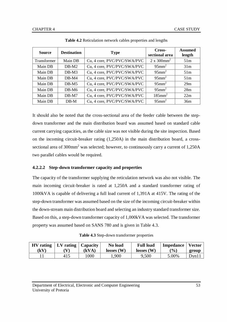
CHAPTER 4 CASE STUDY
Department of Electrical, Electronic and Computer Engineering 53
University of Pretoria
Table 4.2 Reticulation network cables properties and lengths
Source Destination Type Cross-
sectional area
Assumed
length
Transformer Main DB Cu, 4 core, PVC/PVC/SWA/PVC 2 x 300mm2 51m
Main DB DB-M2 Cu, 4 core, PVC/PVC/SWA/PVC 95mm2 31m
Main DB DB-M3 Cu, 4 core, PVC/PVC/SWA/PVC 95mm2 51m
Main DB DB-M4 Cu, 4 core, PVC/PVC/SWA/PVC 95mm2 51m
Main DB DB-M5 Cu, 4 core, PVC/PVC/SWA/PVC 95mm2 29m
Main DB DB-M6 Cu, 4 core, PVC/PVC/SWA/PVC 95mm2 28m
Main DB DB-M7 Cu, 4 core, PVC/PVC/SWA/PVC 185mm2 22m
Main DB DB-M Cu, 4 core, PVC/PVC/SWA/PVC 95mm2 36m
It should also be noted that the cross-sectional area of the feeder cable between the step-
down transformer and the main distribution board was assumed based on standard cable
current carrying capacities, as the cable size was not visible during the site inspection. Based
on the incoming circuit-breaker rating (1,250A) in the main distribution board, a cross-
sectional area of 300mm2 was selected; however, to continuously carry a current of 1,250A
two parallel cables would be required.
4.2.2.2 Step-down transformer capacity and properties
The capacity of the transformer supplying the reticulation network was also not visible. The
main incoming circuit-breaker is rated at 1,250A and a standard transformer rating of
1000kVA is capable of delivering a full load current of 1,391A at 415V. The rating of the
step-down transformer was assumed based on the size of the incoming circuit-breaker within
the down-stream main distribution board and selecting an industry standard transformer size.
Based on this, a step-down transformer capacity of 1,000kVA was selected. The transformer
property was assumed based on SANS 780 and is given in Table 4.3.
Table 4.3 Step-down transformer properties
HV rating
(kV)
LV rating
(V)
Capacity
(kVA)
No load
losses (W)
Full load
losses (W)
Impedance
(%)
Vector
group
11 415 1000 1,900 9,500 5.00% Dyn11
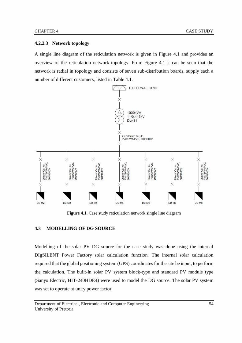
CHAPTER 4 CASE STUDY
Department of Electrical, Electronic and Computer Engineering 54
University of Pretoria
4.2.2.3 Network topology
A single line diagram of the reticulation network is given in Figure 4.1 and provides an
overview of the reticulation network topology. From Figure 4.1 it can be seen that the
network is radial in topology and consists of seven sub-distribution boards, supply each a
number of different customers, listed in Table 4.1.
Figure 4.1. Case study reticulation network single line diagram
4.3 MODELLING OF DG SOURCE
Modelling of the solar PV DG source for the case study was done using the internal
DIgSILENT Power Factory solar calculation function. The internal solar calculation
required that the global positioning system (GPS) coordinates for the site be input, to perform
the calculation. The built-in solar PV system block-type and standard PV module type
(Sanyo Electric, HIT-240HDE4) were used to model the DG source. The solar PV system
was set to operate at unity power factor.
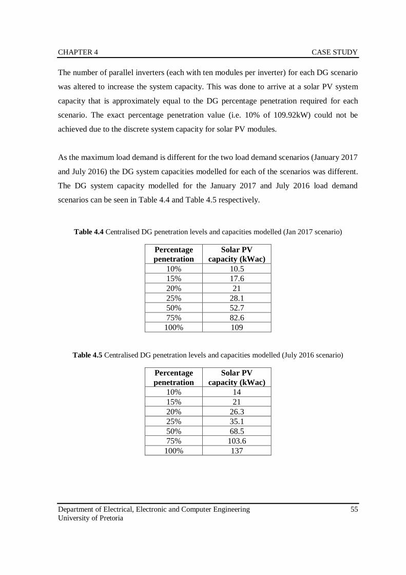
CHAPTER 4 CASE STUDY
Department of Electrical, Electronic and Computer Engineering 55
University of Pretoria
The number of parallel inverters (each with ten modules per inverter) for each DG scenario
was altered to increase the system capacity. This was done to arrive at a solar PV system
capacity that is approximately equal to the DG percentage penetration required for each
scenario. The exact percentage penetration value (i.e. 10% of 109.92kW) could not be
achieved due to the discrete system capacity for solar PV modules.
As the maximum load demand is different for the two load demand scenarios (January 2017
and July 2016) the DG system capacities modelled for each of the scenarios was different.
The DG system capacity modelled for the January 2017 and July 2016 load demand
scenarios can be seen in Table 4.4 and Table 4.5 respectively.
Table 4.4 Centralised DG penetration levels and capacities modelled (Jan 2017 scenario)
Percentage
penetration
Solar PV
capacity (kWac)
10% 10.5
15% 17.6
20% 21
25% 28.1
50% 52.7
75% 82.6
100% 109
Table 4.5 Centralised DG penetration levels and capacities modelled (July 2016 scenario)
Percentage
penetration
Solar PV
capacity (kWac)
10% 14
15% 21
20% 26.3
25% 35.1
50% 68.5
75% 103.6
100% 137
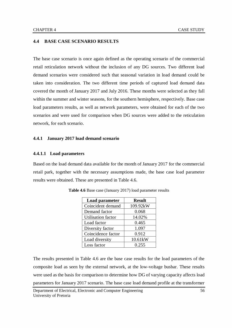
CHAPTER 4 CASE STUDY
Department of Electrical, Electronic and Computer Engineering 56
University of Pretoria
4.4 BASE CASE SCENARIO RESULTS
The base case scenario is once again defined as the operating scenario of the commercial
retail reticulation network without the inclusion of any DG sources. Two different load
demand scenarios were considered such that seasonal variation in load demand could be
taken into consideration. The two different time periods of captured load demand data
covered the month of January 2017 and July 2016. These months were selected as they fall
within the summer and winter seasons, for the southern hemisphere, respectively. Base case
load parameters results, as well as network parameters, were obtained for each of the two
scenarios and were used for comparison when DG sources were added to the reticulation
network, for each scenario.
4.4.1 January 2017 load demand scenario
4.4.1.1 Load parameters
Based on the load demand data available for the month of January 2017 for the commercial
retail park, together with the necessary assumptions made, the base case load parameter
results were obtained. These are presented in Table 4.6.
Table 4.6 Base case (January 2017) load parameter results
Load parameter Result
Coincident demand 109.92kW
Demand factor 0.068
Utilisation factor 14.02%
Load factor 0.465
Diversity factor 1.097
Coincidence factor 0.912
Load diversity 10.61kW
Loss factor 0.255
The results presented in Table 4.6 are the base case results for the load parameters of the
composite load as seen by the external network, at the low-voltage busbar. These results
were used as the basis for comparison to determine how DG of varying capacity affects load
parameters for January 2017 scenario. The base case load demand profile at the transformer
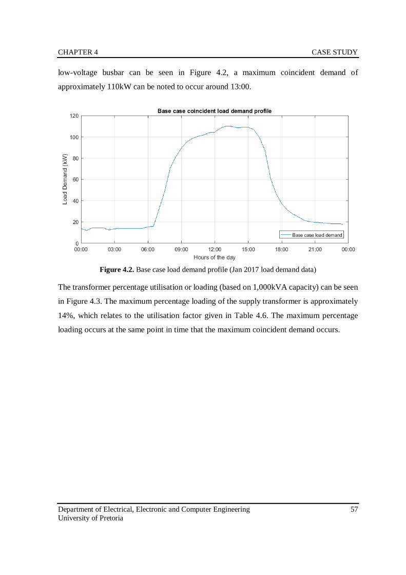
CHAPTER 4 CASE STUDY
Department of Electrical, Electronic and Computer Engineering 57
University of Pretoria
low-voltage busbar can be seen in Figure 4.2, a maximum coincident demand of
approximately 110kW can be noted to occur around 13:00.
Figure 4.2. Base case load demand profile (Jan 2017 load demand data)
The transformer percentage utilisation or loading (based on 1,000kVA capacity) can be seen
in Figure 4.3. The maximum percentage loading of the supply transformer is approximately
14%, which relates to the utilisation factor given in Table 4.6. The maximum percentage
loading occurs at the same point in time that the maximum coincident demand occurs.
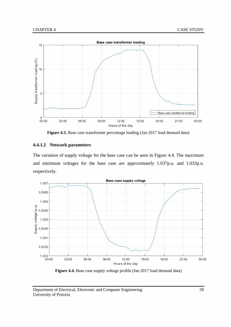
CHAPTER 4 CASE STUDY
Department of Electrical, Electronic and Computer Engineering 58
University of Pretoria
Figure 4.3. Base case transformer percentage loading (Jan 2017 load demand data)
4.4.1.2 Network parameters
The variation of supply voltage for the base case can be seen in Figure 4.4. The maximum
and minimum voltages for the base case are approximately 1.037p.u. and 1.033p.u.
respectively.
Figure 4.4. Base case supply voltage profile (Jan 2017 load demand data)
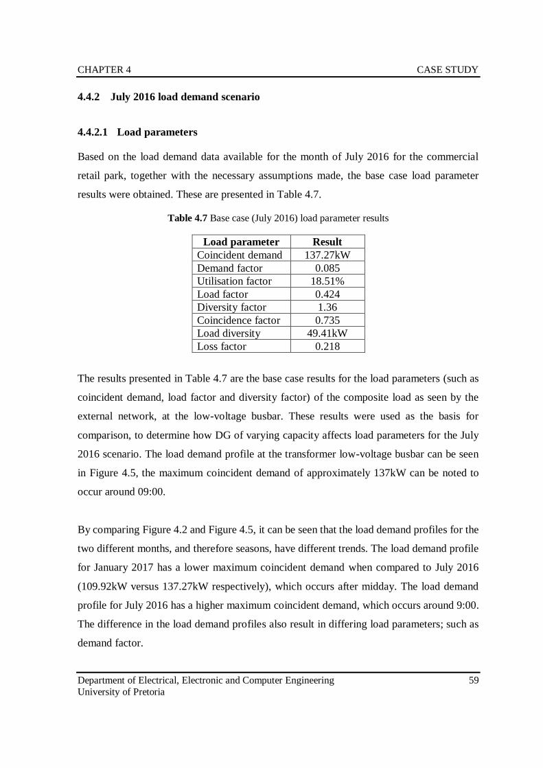
CHAPTER 4 CASE STUDY
Department of Electrical, Electronic and Computer Engineering 59
University of Pretoria
4.4.2 July 2016 load demand scenario
4.4.2.1 Load parameters
Based on the load demand data available for the month of July 2016 for the commercial
retail park, together with the necessary assumptions made, the base case load parameter
results were obtained. These are presented in Table 4.7.
Table 4.7 Base case (July 2016) load parameter results
Load parameter Result
Coincident demand 137.27kW
Demand factor 0.085
Utilisation factor 18.51%
Load factor 0.424
Diversity factor 1.36
Coincidence factor 0.735
Load diversity 49.41kW
Loss factor 0.218
The results presented in Table 4.7 are the base case results for the load parameters (such as
coincident demand, load factor and diversity factor) of the composite load as seen by the
external network, at the low-voltage busbar. These results were used as the basis for
comparison, to determine how DG of varying capacity affects load parameters for the July
2016 scenario. The load demand profile at the transformer low-voltage busbar can be seen
in Figure 4.5, the maximum coincident demand of approximately 137kW can be noted to
occur around 09:00.
By comparing Figure 4.2 and Figure 4.5, it can be seen that the load demand profiles for the
two different months, and therefore seasons, have different trends. The load demand profile
for January 2017 has a lower maximum coincident demand when compared to July 2016
(109.92kW versus 137.27kW respectively), which occurs after midday. The load demand
profile for July 2016 has a higher maximum coincident demand, which occurs around 9:00.
The difference in the load demand profiles also result in differing load parameters; such as
demand factor.
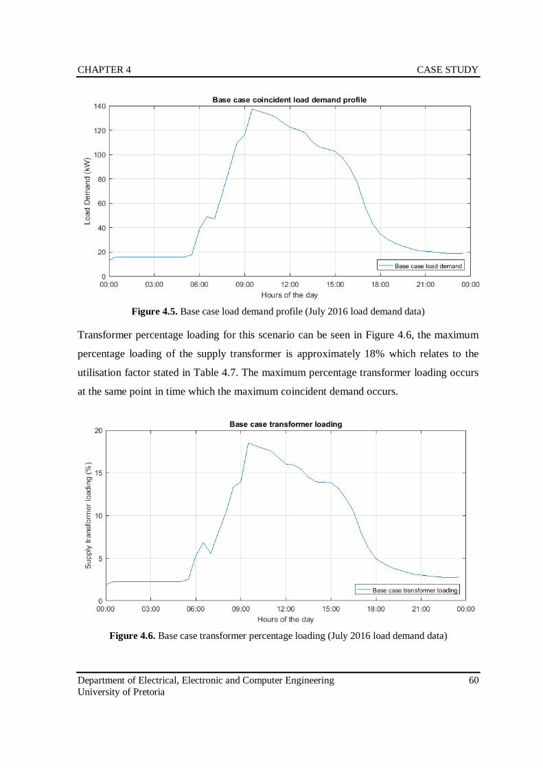
CHAPTER 4 CASE STUDY
Department of Electrical, Electronic and Computer Engineering 60
University of Pretoria
Figure 4.5. Base case load demand profile (July 2016 load demand data)
Transformer percentage loading for this scenario can be seen in Figure 4.6, the maximum
percentage loading of the supply transformer is approximately 18% which relates to the
utilisation factor stated in Table 4.7. The maximum percentage transformer loading occurs
at the same point in time which the maximum coincident demand occurs.
Figure 4.6. Base case transformer percentage loading (July 2016 load demand data)
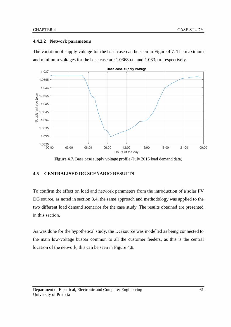
CHAPTER 4 CASE STUDY
Department of Electrical, Electronic and Computer Engineering 61
University of Pretoria
4.4.2.2 Network parameters
The variation of supply voltage for the base case can be seen in Figure 4.7. The maximum
and minimum voltages for the base case are 1.0368p.u. and 1.033p.u. respectively.
Figure 4.7. Base case supply voltage profile (July 2016 load demand data)
4.5 CENTRALISED DG SCENARIO RESULTS
To confirm the effect on load and network parameters from the introduction of a solar PV
DG source, as noted in section 3.4, the same approach and methodology was applied to the
two different load demand scenarios for the case study. The results obtained are presented
in this section.
As was done for the hypothetical study, the DG source was modelled as being connected to
the main low-voltage busbar common to all the customer feeders, as this is the central
location of the network, this can be seen in Figure 4.8.
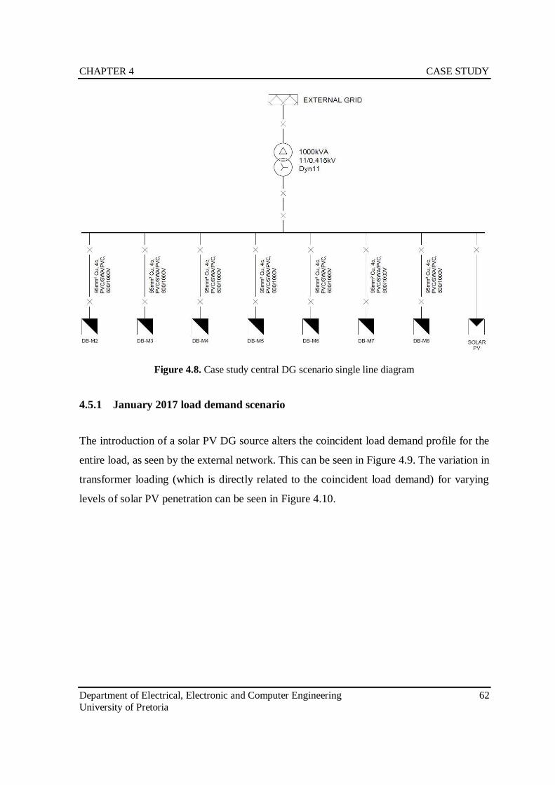
CHAPTER 4 CASE STUDY
Department of Electrical, Electronic and Computer Engineering 62
University of Pretoria
Figure 4.8. Case study central DG scenario single line diagram
4.5.1 January 2017 load demand scenario
The introduction of a solar PV DG source alters the coincident load demand profile for the
entire load, as seen by the external network. This can be seen in Figure 4.9. The variation in
transformer loading (which is directly related to the coincident load demand) for varying
levels of solar PV penetration can be seen in Figure 4.10.
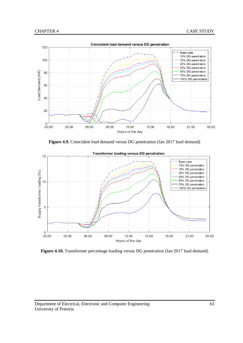
CHAPTER 4 CASE STUDY
Department of Electrical, Electronic and Computer Engineering 63
University of Pretoria
Figure 4.9. Coincident load demand versus DG penetration (Jan 2017 load demand)
Figure 4.10. Transformer percentage loading versus DG penetration (Jan 2017 load demand)
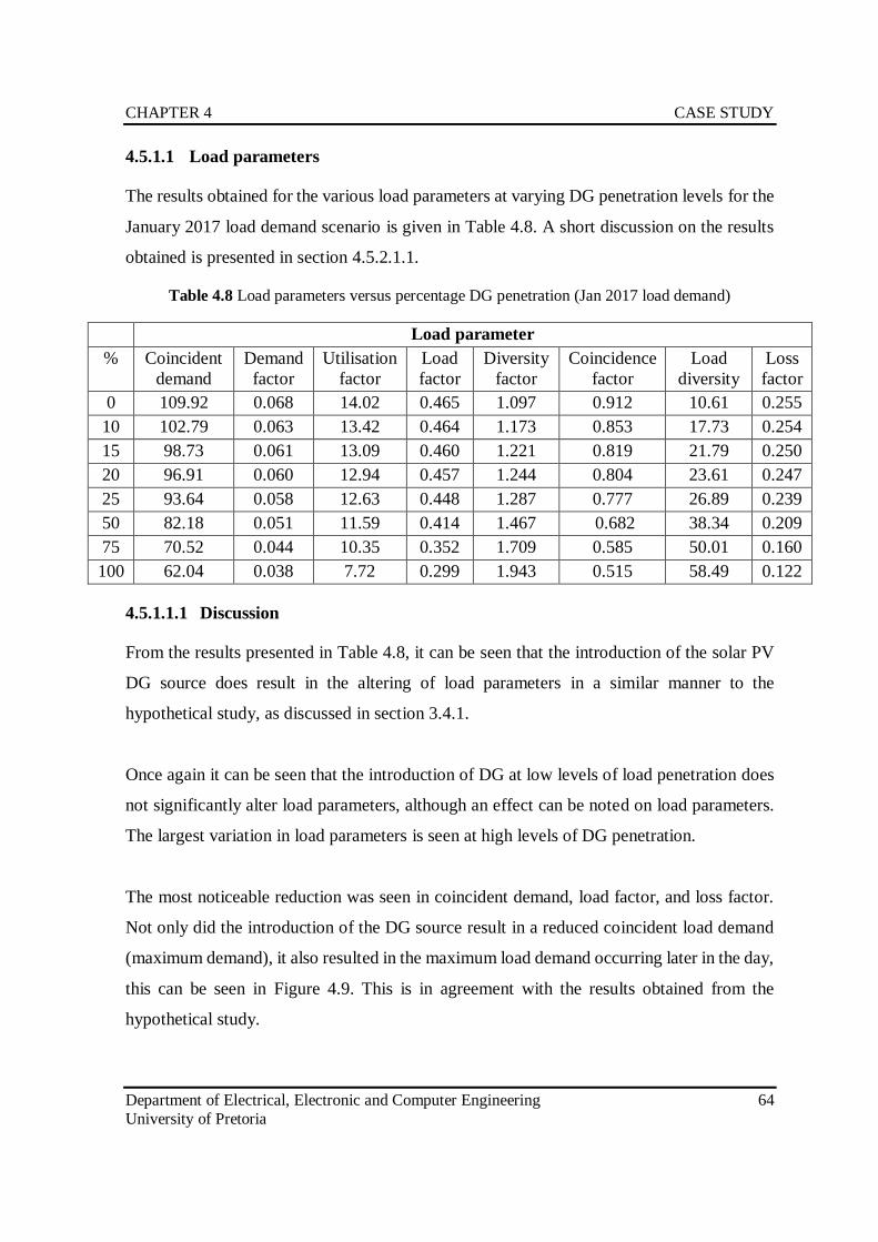
CHAPTER 4 CASE STUDY
Department of Electrical, Electronic and Computer Engineering 64
University of Pretoria
4.5.1.1 Load parameters
The results obtained for the various load parameters at varying DG penetration levels for the
January 2017 load demand scenario is given in Table 4.8. A short discussion on the results
obtained is presented in section 4.5.2.1.1.
Table 4.8 Load parameters versus percentage DG penetration (Jan 2017 load demand)
Load parameter
% Coincident
demand
Demand
factor
Utilisation
factor
Load
factor
Diversity
factor
Coincidence
factor
Load
diversity
Loss
factor
0 109.92 0.068 14.02 0.465 1.097 0.912 10.61 0.255
10 102.79 0.063 13.42 0.464 1.173 0.853 17.73 0.254
15 98.73 0.061 13.09 0.460 1.221 0.819 21.79 0.250
20 96.91 0.060 12.94 0.457 1.244 0.804 23.61 0.247
25 93.64 0.058 12.63 0.448 1.287 0.777 26.89 0.239
50 82.18 0.051 11.59 0.414 1.467 0.682 38.34 0.209
75 70.52 0.044 10.35 0.352 1.709 0.585 50.01 0.160
100 62.04 0.038 7.72 0.299 1.943 0.515 58.49 0.122
4.5.1.1.1 Discussion
From the results presented in Table 4.8, it can be seen that the introduction of the solar PV
DG source does result in the altering of load parameters in a similar manner to the
hypothetical study, as discussed in section 3.4.1.
Once again it can be seen that the introduction of DG at low levels of load penetration does
not significantly alter load parameters, although an effect can be noted on load parameters.
The largest variation in load parameters is seen at high levels of DG penetration.
The most noticeable reduction was seen in coincident demand, load factor, and loss factor.
Not only did the introduction of the DG source result in a reduced coincident load demand
(maximum demand), it also resulted in the maximum load demand occurring later in the day,
this can be seen in Figure 4.9. This is in agreement with the results obtained from the
hypothetical study.
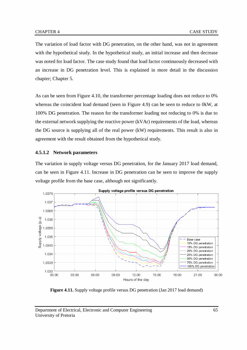
CHAPTER 4 CASE STUDY
Department of Electrical, Electronic and Computer Engineering 65
University of Pretoria
The variation of load factor with DG penetration, on the other hand, was not in agreement
with the hypothetical study. In the hypothetical study, an initial increase and then decrease
was noted for load factor. The case study found that load factor continuously decreased with
an increase in DG penetration level. This is explained in more detail in the discussion
chapter; Chapter 5.
As can be seen from Figure 4.10, the transformer percentage loading does not reduce to 0%
whereas the coincident load demand (seen in Figure 4.9) can be seen to reduce to 0kW, at
100% DG penetration. The reason for the transformer loading not reducing to 0% is due to
the external network supplying the reactive power (kVAr) requirements of the load, whereas
the DG source is supplying all of the real power (kW) requirements. This result is also in
agreement with the result obtained from the hypothetical study.
4.5.1.2 Network parameters
The variation in supply voltage versus DG penetration, for the January 2017 load demand,
can be seen in Figure 4.11. Increase in DG penetration can be seen to improve the supply
voltage profile from the base case, although not significantly.
Figure 4.11. Supply voltage profile versus DG penetration (Jan 2017 load demand)
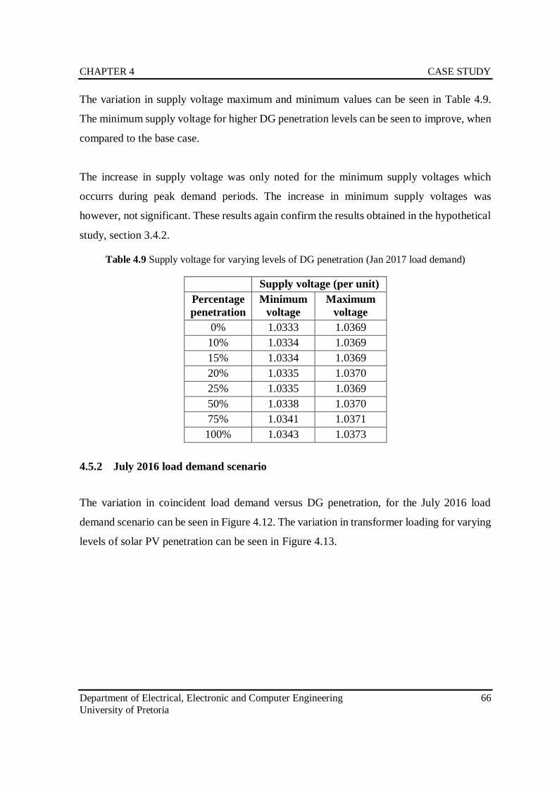
CHAPTER 4 CASE STUDY
Department of Electrical, Electronic and Computer Engineering 66
University of Pretoria
The variation in supply voltage maximum and minimum values can be seen in Table 4.9.
The minimum supply voltage for higher DG penetration levels can be seen to improve, when
compared to the base case.
The increase in supply voltage was only noted for the minimum supply voltages which
occurrs during peak demand periods. The increase in minimum supply voltages was
however, not significant. These results again confirm the results obtained in the hypothetical
study, section 3.4.2.
Table 4.9 Supply voltage for varying levels of DG penetration (Jan 2017 load demand)
Supply voltage (per unit)
Percentage
penetration
Minimum
voltage
Maximum
voltage
0% 1.0333 1.0369
10% 1.0334 1.0369
15% 1.0334 1.0369
20% 1.0335 1.0370
25% 1.0335 1.0369
50% 1.0338 1.0370
75% 1.0341 1.0371
100% 1.0343 1.0373
4.5.2 July 2016 load demand scenario
The variation in coincident load demand versus DG penetration, for the July 2016 load
demand scenario can be seen in Figure 4.12. The variation in transformer loading for varying
levels of solar PV penetration can be seen in Figure 4.13.
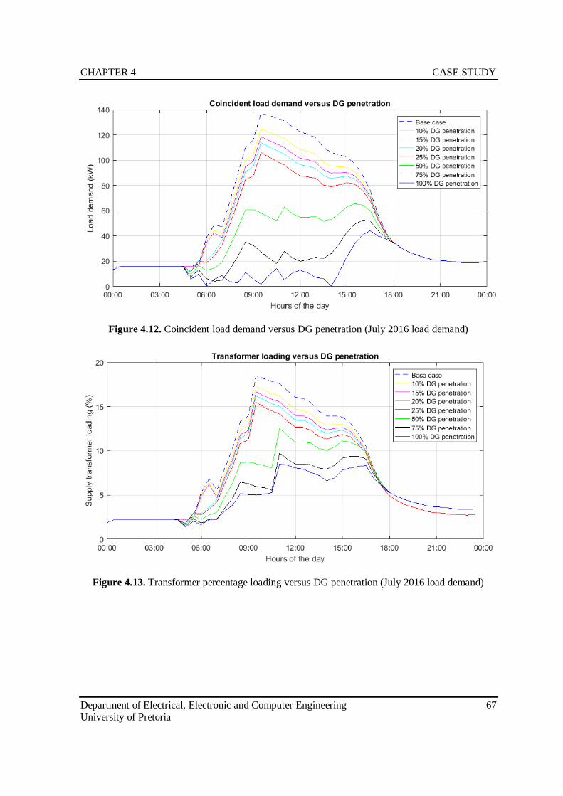
CHAPTER 4 CASE STUDY
Department of Electrical, Electronic and Computer Engineering 67
University of Pretoria
Figure 4.12. Coincident load demand versus DG penetration (July 2016 load demand)
Figure 4.13. Transformer percentage loading versus DG penetration (July 2016 load demand)
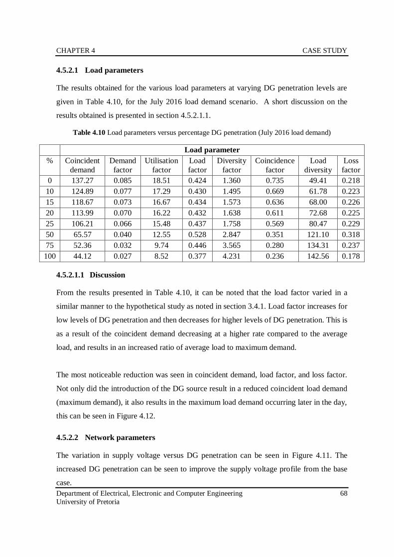
CHAPTER 4 CASE STUDY
Department of Electrical, Electronic and Computer Engineering 68
University of Pretoria
4.5.2.1 Load parameters
The results obtained for the various load parameters at varying DG penetration levels are
given in Table 4.10, for the July 2016 load demand scenario. A short discussion on the
results obtained is presented in section 4.5.2.1.1.
Table 4.10 Load parameters versus percentage DG penetration (July 2016 load demand)
Load parameter
% Coincident
demand
Demand
factor
Utilisation
factor
Load
factor
Diversity
factor
Coincidence
factor
Load
diversity
Loss
factor
0 137.27 0.085 18.51 0.424 1.360 0.735 49.41 0.218
10 124.89 0.077 17.29 0.430 1.495 0.669 61.78 0.223
15 118.67 0.073 16.67 0.434 1.573 0.636 68.00 0.226
20 113.99 0.070 16.22 0.432 1.638 0.611 72.68 0.225
25 106.21 0.066 15.48 0.437 1.758 0.569 80.47 0.229
50 65.57 0.040 12.55 0.528 2.847 0.351 121.10 0.318
75 52.36 0.032 9.74 0.446 3.565 0.280 134.31 0.237
100 44.12 0.027 8.52 0.377 4.231 0.236 142.56 0.178
4.5.2.1.1 Discussion
From the results presented in Table 4.10, it can be noted that the load factor varied in a
similar manner to the hypothetical study as noted in section 3.4.1. Load factor increases for
low levels of DG penetration and then decreases for higher levels of DG penetration. This is
as a result of the coincident demand decreasing at a higher rate compared to the average
load, and results in an increased ratio of average load to maximum demand.
The most noticeable reduction was seen in coincident demand, load factor, and loss factor.
Not only did the introduction of the DG source result in a reduced coincident load demand
(maximum demand), it also results in the maximum load demand occurring later in the day,
this can be seen in Figure 4.12.
4.5.2.2 Network parameters
The variation in supply voltage versus DG penetration can be seen in Figure 4.11. The
increased DG penetration can be seen to improve the supply voltage profile from the base
case.
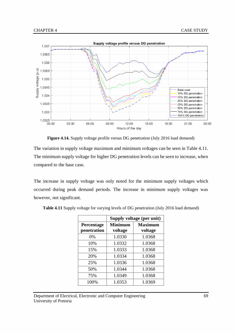
CHAPTER 4 CASE STUDY
Department of Electrical, Electronic and Computer Engineering 69
University of Pretoria
Figure 4.14. Supply voltage profile versus DG penetration (July 2016 load demand)
The variation in supply voltage maximum and minimum voltages can be seen in Table 4.11.
The minimum supply voltage for higher DG penetration levels can be seen to increase, when
compared to the base case.
The increase in supply voltage was only noted for the minimum supply voltages which
occurred during peak demand periods. The increase in minimum supply voltages was
however, not significant.
Table 4.11 Supply voltage for varying levels of DG penetration (July 2016 load demand)
Supply voltage (per unit)
Percentage
penetration
Minimum
voltage
Maximum
voltage
0% 1.0330 1.0368
10% 1.0332 1.0368
15% 1.0333 1.0368
20% 1.0334 1.0368
25% 1.0336 1.0368
50% 1.0344 1.0368
75% 1.0349 1.0368
100% 1.0353 1.0369
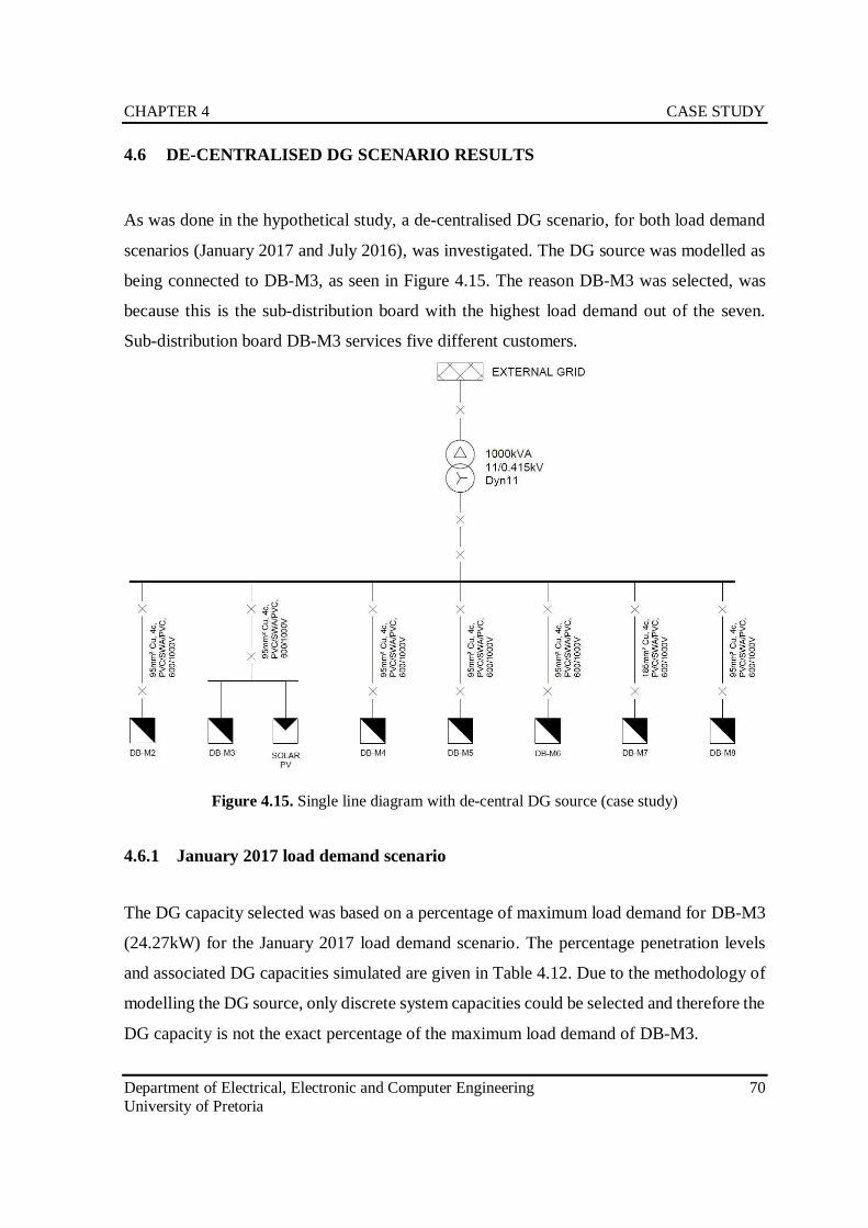
CHAPTER 4 CASE STUDY
Department of Electrical, Electronic and Computer Engineering 70
University of Pretoria
4.6 DE-CENTRALISED DG SCENARIO RESULTS
As was done in the hypothetical study, a de-centralised DG scenario, for both load demand
scenarios (January 2017 and July 2016), was investigated. The DG source was modelled as
being connected to DB-M3, as seen in Figure 4.15. The reason DB-M3 was selected, was
because this is the sub-distribution board with the highest load demand out of the seven.
Sub-distribution board DB-M3 services five different customers.
Figure 4.15. Single line diagram with de-central DG source (case study)
4.6.1 January 2017 load demand scenario
The DG capacity selected was based on a percentage of maximum load demand for DB-M3
(24.27kW) for the January 2017 load demand scenario. The percentage penetration levels
and associated DG capacities simulated are given in Table 4.12. Due to the methodology of
modelling the DG source, only discrete system capacities could be selected and therefore the
DG capacity is not the exact percentage of the maximum load demand of DB-M3.
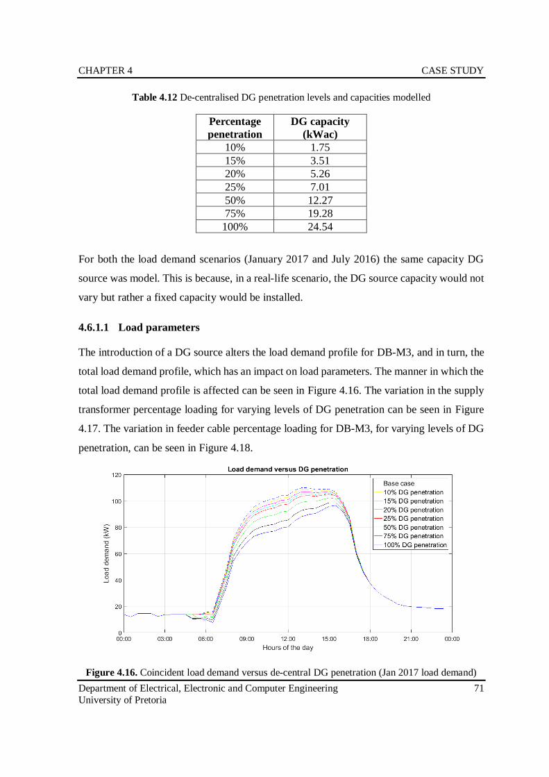
CHAPTER 4 CASE STUDY
Department of Electrical, Electronic and Computer Engineering 71
University of Pretoria
Table 4.12 De-centralised DG penetration levels and capacities modelled
Percentage
penetration
DG capacity
(kWac)
10% 1.75
15% 3.51
20% 5.26
25% 7.01
50% 12.27
75% 19.28
100% 24.54
For both the load demand scenarios (January 2017 and July 2016) the same capacity DG
source was model. This is because, in a real-life scenario, the DG source capacity would not
vary but rather a fixed capacity would be installed.
4.6.1.1 Load parameters
The introduction of a DG source alters the load demand profile for DB-M3, and in turn, the
total load demand profile, which has an impact on load parameters. The manner in which the
total load demand profile is affected can be seen in Figure 4.16. The variation in the supply
transformer percentage loading for varying levels of DG penetration can be seen in Figure
4.17. The variation in feeder cable percentage loading for DB-M3, for varying levels of DG
penetration, can be seen in Figure 4.18.
Figure 4.16. Coincident load demand versus de-central DG penetration (Jan 2017 load demand)
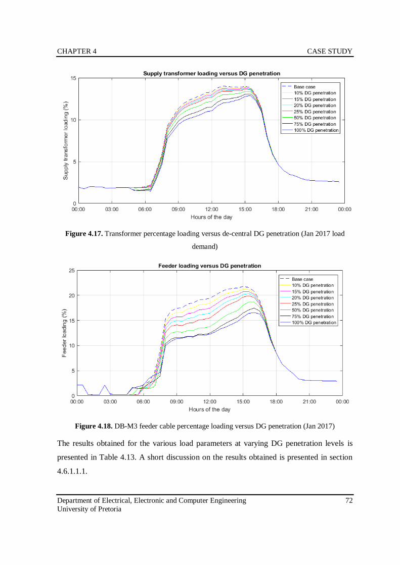
CHAPTER 4 CASE STUDY
Department of Electrical, Electronic and Computer Engineering 72
University of Pretoria
Figure 4.17. Transformer percentage loading versus de-central DG penetration (Jan 2017 load
demand)
Figure 4.18. DB-M3 feeder cable percentage loading versus DG penetration (Jan 2017)
The results obtained for the various load parameters at varying DG penetration levels is
presented in Table 4.13. A short discussion on the results obtained is presented in section
4.6.1.1.1.
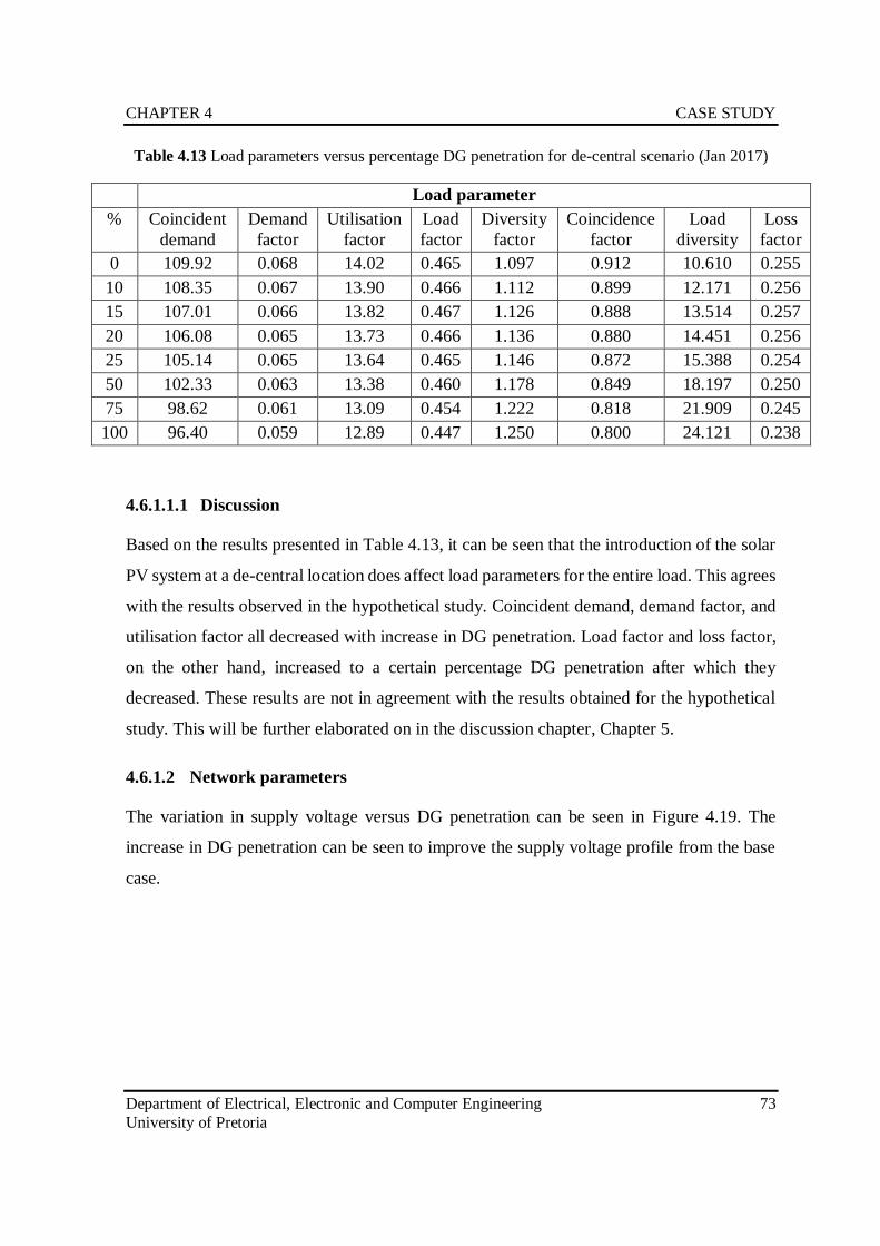
CHAPTER 4 CASE STUDY
Department of Electrical, Electronic and Computer Engineering 73
University of Pretoria
Table 4.13 Load parameters versus percentage DG penetration for de-central scenario (Jan 2017)
Load parameter
% Coincident
demand
Demand
factor
Utilisation
factor
Load
factor
Diversity
factor
Coincidence
factor
Load
diversity
Loss
factor
0 109.92 0.068 14.02 0.465 1.097 0.912 10.610 0.255
10 108.35 0.067 13.90 0.466 1.112 0.899 12.171 0.256
15 107.01 0.066 13.82 0.467 1.126 0.888 13.514 0.257
20 106.08 0.065 13.73 0.466 1.136 0.880 14.451 0.256
25 105.14 0.065 13.64 0.465 1.146 0.872 15.388 0.254
50 102.33 0.063 13.38 0.460 1.178 0.849 18.197 0.250
75 98.62 0.061 13.09 0.454 1.222 0.818 21.909 0.245
100 96.40 0.059 12.89 0.447 1.250 0.800 24.121 0.238
4.6.1.1.1 Discussion
Based on the results presented in Table 4.13, it can be seen that the introduction of the solar
PV system at a de-central location does affect load parameters for the entire load. This agrees
with the results observed in the hypothetical study. Coincident demand, demand factor, and
utilisation factor all decreased with increase in DG penetration. Load factor and loss factor,
on the other hand, increased to a certain percentage DG penetration after which they
decreased. These results are not in agreement with the results obtained for the hypothetical
study. This will be further elaborated on in the discussion chapter, Chapter 5.
4.6.1.2 Network parameters
The variation in supply voltage versus DG penetration can be seen in Figure 4.19. The
increase in DG penetration can be seen to improve the supply voltage profile from the base
case.
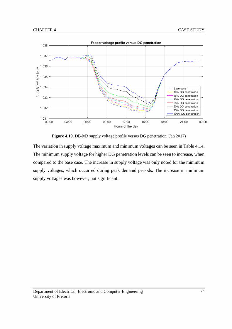
CHAPTER 4 CASE STUDY
Department of Electrical, Electronic and Computer Engineering 74
University of Pretoria
Figure 4.19. DB-M3 supply voltage profile versus DG penetration (Jan 2017)
The variation in supply voltage maximum and minimum voltages can be seen in Table 4.14.
The minimum supply voltage for higher DG penetration levels can be seen to increase, when
compared to the base case. The increase in supply voltage was only noted for the minimum
supply voltages, which occurred during peak demand periods. The increase in minimum
supply voltages was however, not significant.
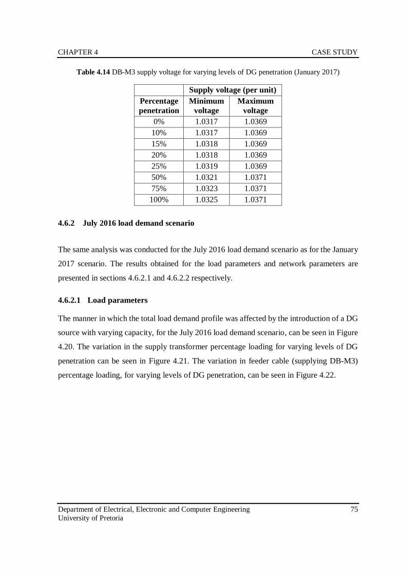
CHAPTER 4 CASE STUDY
Department of Electrical, Electronic and Computer Engineering 75
University of Pretoria
Table 4.14 DB-M3 supply voltage for varying levels of DG penetration (January 2017)
Supply voltage (per unit)
Percentage
penetration
Minimum
voltage
Maximum
voltage
0% 1.0317 1.0369
10% 1.0317 1.0369
15% 1.0318 1.0369
20% 1.0318 1.0369
25% 1.0319 1.0369
50% 1.0321 1.0371
75% 1.0323 1.0371
100% 1.0325 1.0371
4.6.2 July 2016 load demand scenario
The same analysis was conducted for the July 2016 load demand scenario as for the January
2017 scenario. The results obtained for the load parameters and network parameters are
presented in sections 4.6.2.1 and 4.6.2.2 respectively.
4.6.2.1 Load parameters
The manner in which the total load demand profile was affected by the introduction of a DG
source with varying capacity, for the July 2016 load demand scenario, can be seen in Figure
4.20. The variation in the supply transformer percentage loading for varying levels of DG
penetration can be seen in Figure 4.21. The variation in feeder cable (supplying DB-M3)
percentage loading, for varying levels of DG penetration, can be seen in Figure 4.22.
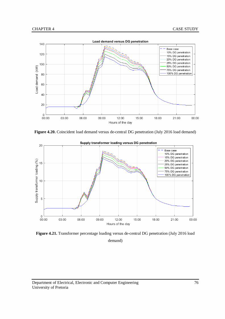
CHAPTER 4 CASE STUDY
Department of Electrical, Electronic and Computer Engineering 76
University of Pretoria
Figure 4.20. Coincident load demand versus de-central DG penetration (July 2016 load demand)
Figure 4.21. Transformer percentage loading versus de-central DG penetration (July 2016 load
demand)
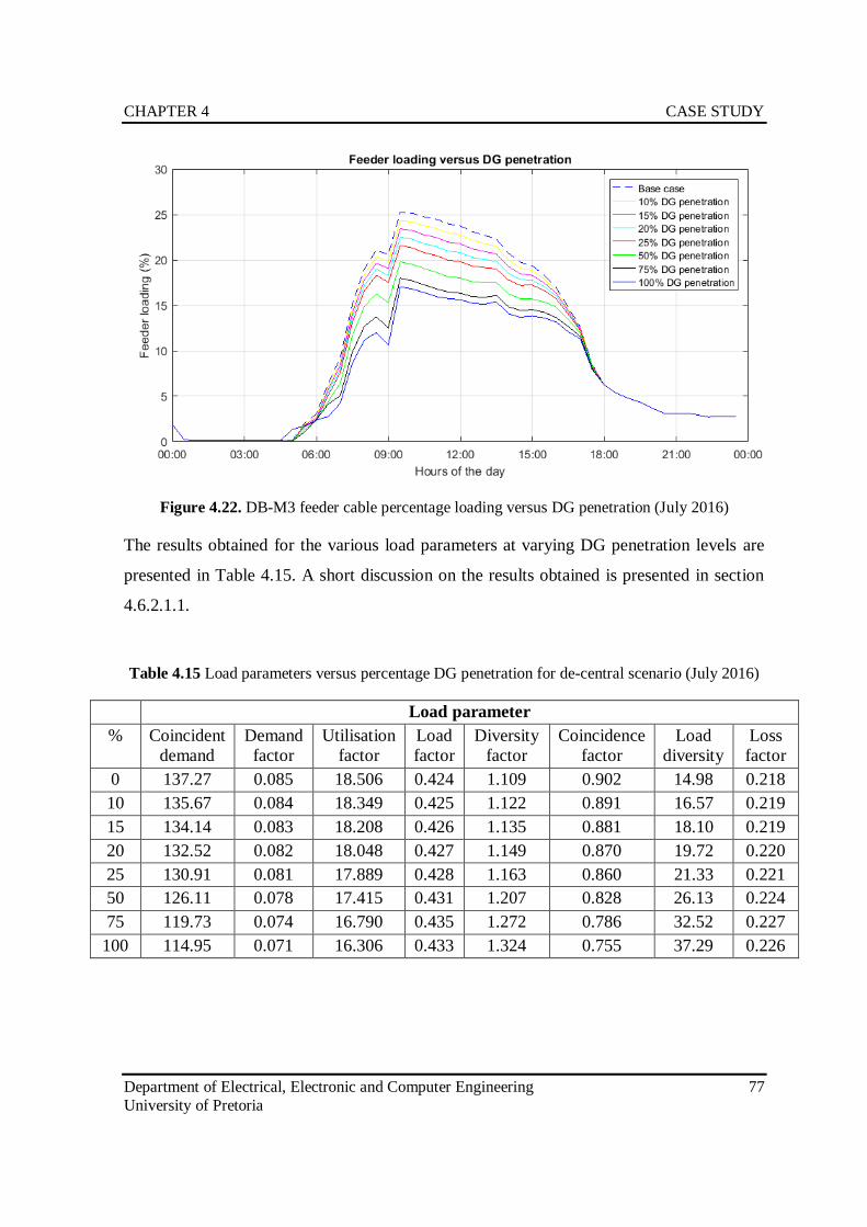
CHAPTER 4 CASE STUDY
Department of Electrical, Electronic and Computer Engineering 77
University of Pretoria
Figure 4.22. DB-M3 feeder cable percentage loading versus DG penetration (July 2016)
The results obtained for the various load parameters at varying DG penetration levels are
presented in Table 4.15. A short discussion on the results obtained is presented in section
4.6.2.1.1.
Table 4.15 Load parameters versus percentage DG penetration for de-central scenario (July 2016)
Load parameter
% Coincident
demand
Demand
factor
Utilisation
factor
Load
factor
Diversity
factor
Coincidence
factor
Load
diversity
Loss
factor
0 137.27 0.085 18.506 0.424 1.109 0.902 14.98 0.218
10 135.67 0.084 18.349 0.425 1.122 0.891 16.57 0.219
15 134.14 0.083 18.208 0.426 1.135 0.881 18.10 0.219
20 132.52 0.082 18.048 0.427 1.149 0.870 19.72 0.220
25 130.91 0.081 17.889 0.428 1.163 0.860 21.33 0.221
50 126.11 0.078 17.415 0.431 1.207 0.828 26.13 0.224
75 119.73 0.074 16.790 0.435 1.272 0.786 32.52 0.227
100 114.95 0.071 16.306 0.433 1.324 0.755 37.29 0.226
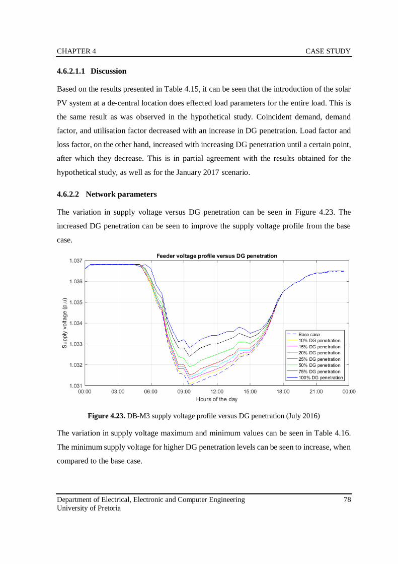
CHAPTER 4 CASE STUDY
Department of Electrical, Electronic and Computer Engineering 78
University of Pretoria
4.6.2.1.1 Discussion
Based on the results presented in Table 4.15, it can be seen that the introduction of the solar
PV system at a de-central location does effected load parameters for the entire load. This is
the same result as was observed in the hypothetical study. Coincident demand, demand
factor, and utilisation factor decreased with an increase in DG penetration. Load factor and
loss factor, on the other hand, increased with increasing DG penetration until a certain point,
after which they decrease. This is in partial agreement with the results obtained for the
hypothetical study, as well as for the January 2017 scenario.
4.6.2.2 Network parameters
The variation in supply voltage versus DG penetration can be seen in Figure 4.23. The
increased DG penetration can be seen to improve the supply voltage profile from the base
case.
Figure 4.23. DB-M3 supply voltage profile versus DG penetration (July 2016)
The variation in supply voltage maximum and minimum values can be seen in Table 4.16.
The minimum supply voltage for higher DG penetration levels can be seen to increase, when
compared to the base case.
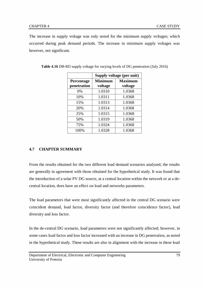
CHAPTER 4 CASE STUDY
Department of Electrical, Electronic and Computer Engineering 79
University of Pretoria
The increase in supply voltage was only noted for the minimum supply voltages; which
occurred during peak demand periods. The increase in minimum supply voltages was
however, not significant.
Table 4.16 DB-M3 supply voltage for varying levels of DG penetration (July 2016)
Supply voltage (per unit)
Percentage
penetration
Minimum
voltage
Maximum
voltage
0% 1.0310 1.0368
10% 1.0311 1.0368
15% 1.0313 1.0368
20% 1.0314 1.0368
25% 1.0315 1.0368
50% 1.0319 1.0368
75% 1.0324 1.0368
100% 1.0328 1.0368
4.7 CHAPTER SUMMARY
From the results obtained for the two different load demand scenarios analysed, the results
are generally in agreement with those obtained for the hypothetical study. It was found that
the introduction of a solar PV DG source, at a central location within the network or at a de-
central location, does have an effect on load and networks parameters.
The load parameters that were most significantly affected in the central DG scenario were
coincident demand, load factor, diversity factor (and therefore coincidence factor), load
diversity and loss factor.
In the de-central DG scenario, load parameters were not significantly affected; however, in
some cases load factor and loss factor increased with an increase in DG penetration, as noted
in the hypothetical study. These results are also in alignment with the increase in these load

CHAPTER 4 CASE STUDY
Department of Electrical, Electronic and Computer Engineering 80
University of Pretoria
parameters (for the central DG scenario) for low levels of DG penetration in the July 2016
load demand case.
Network parameters, such as supply voltage, for both the central and de-central DG scenario
were not significantly affected by varying levels of DG penetration. This is in agreement
with the results obtained for the hypothetical study.
CHAPTER 5 DISCUSSION
5.1 CHAPTER OVERVIEW
The objective of this chapter is to discuss the results obtained for the hypothetical study and
the case study. The results will be compared for validation and further analysed to determine
the impact that varying levels of DG penetration has on load and network parameters. In
addition to this, a conclusion will be made as to whether the impact on load and network
parameters is great enough to warrant further investigation into determining suitable
planning and design standards for reticulation networks containing varying levels of DG
penetration.
5.2 HYPOTHETICAL STUDY
The impact of varying levels of DG penetration on load and networks parameters, for the
hypothetical study, are further discussed in section 5.2.1 and 5.2.2 respectively.
5.2.1 Load parameters
The impact of varying levels of DG penetration on each of the load parameters under
investigation are discussed below, for both the central and de-central DG scenarios.
5.2.1.1 Coincident demand
5.2.1.1.1 Central DG scenario
The impact of varying levels of DG penetration on coincident demand for the central DG
scenario is given in Figure 5.1. The variation in DG penetration from 0% to 100% (0kW to
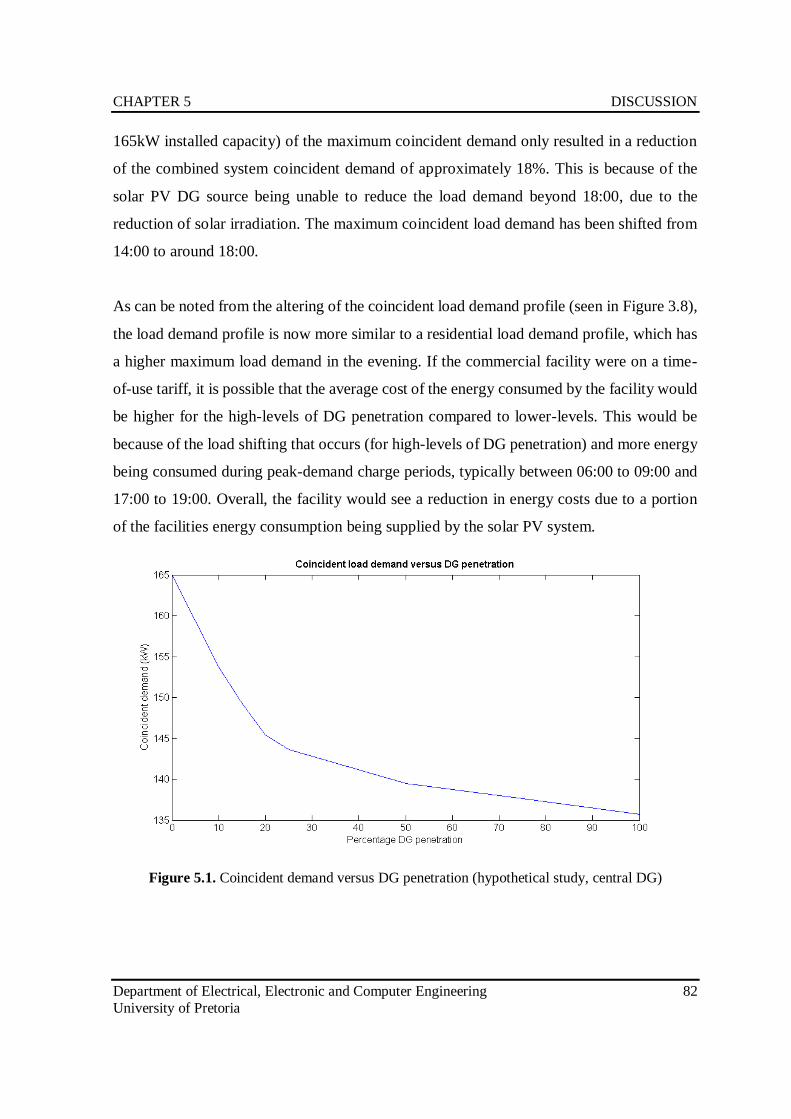
CHAPTER 5 DISCUSSION
Department of Electrical, Electronic and Computer Engineering 82
University of Pretoria
165kW installed capacity) of the maximum coincident demand only resulted in a reduction
of the combined system coincident demand of approximately 18%. This is because of the
solar PV DG source being unable to reduce the load demand beyond 18:00, due to the
reduction of solar irradiation. The maximum coincident load demand has been shifted from
14:00 to around 18:00.
As can be noted from the altering of the coincident load demand profile (seen in Figure 3.8),
the load demand profile is now more similar to a residential load demand profile, which has
a higher maximum load demand in the evening. If the commercial facility were on a time-
of-use tariff, it is possible that the average cost of the energy consumed by the facility would
be higher for the high-levels of DG penetration compared to lower-levels. This would be
because of the load shifting that occurs (for high-levels of DG penetration) and more energy
being consumed during peak-demand charge periods, typically between 06:00 to 09:00 and
17:00 to 19:00. Overall, the facility would see a reduction in energy costs due to a portion
of the facilities energy consumption being supplied by the solar PV system.
Figure 5.1. Coincident demand versus DG penetration (hypothetical study, central DG)
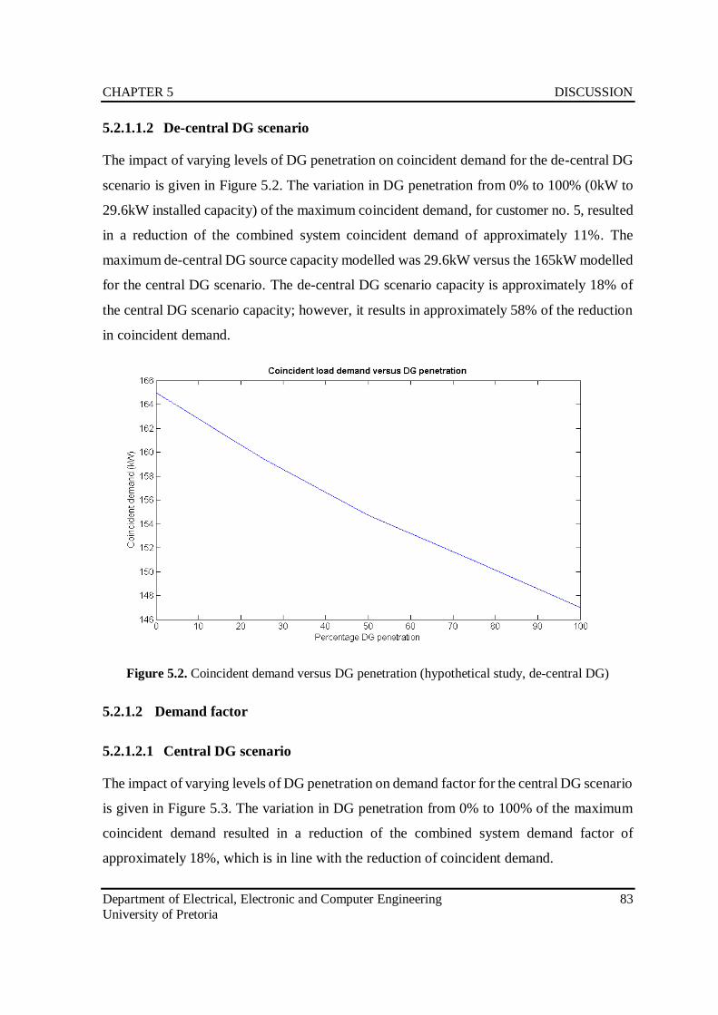
CHAPTER 5 DISCUSSION
Department of Electrical, Electronic and Computer Engineering 83
University of Pretoria
5.2.1.1.2 De-central DG scenario
The impact of varying levels of DG penetration on coincident demand for the de-central DG
scenario is given in Figure 5.2. The variation in DG penetration from 0% to 100% (0kW to
29.6kW installed capacity) of the maximum coincident demand, for customer no. 5, resulted
in a reduction of the combined system coincident demand of approximately 11%. The
maximum de-central DG source capacity modelled was 29.6kW versus the 165kW modelled
for the central DG scenario. The de-central DG scenario capacity is approximately 18% of
the central DG scenario capacity; however, it results in approximately 58% of the reduction
in coincident demand.
Figure 5.2. Coincident demand versus DG penetration (hypothetical study, de-central DG)
5.2.1.2 Demand factor
5.2.1.2.1 Central DG scenario
The impact of varying levels of DG penetration on demand factor for the central DG scenario
is given in Figure 5.3. The variation in DG penetration from 0% to 100% of the maximum
coincident demand resulted in a reduction of the combined system demand factor of
approximately 18%, which is in line with the reduction of coincident demand.
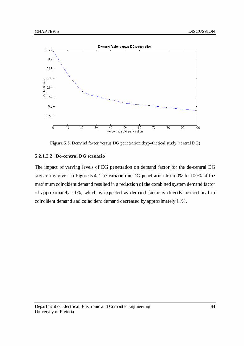
CHAPTER 5 DISCUSSION
Department of Electrical, Electronic and Computer Engineering 84
University of Pretoria
Figure 5.3. Demand factor versus DG penetration (hypothetical study, central DG)
5.2.1.2.2 De-central DG scenario
The impact of varying levels of DG penetration on demand factor for the de-central DG
scenario is given in Figure 5.4. The variation in DG penetration from 0% to 100% of the
maximum coincident demand resulted in a reduction of the combined system demand factor
of approximately 11%, which is expected as demand factor is directly proportional to
coincident demand and coincident demand decreased by approximately 11%.
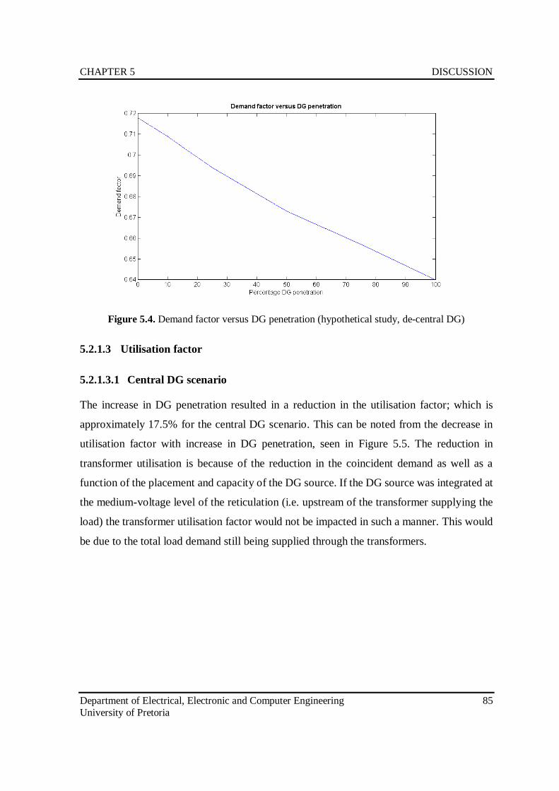
CHAPTER 5 DISCUSSION
Department of Electrical, Electronic and Computer Engineering 85
University of Pretoria
Figure 5.4. Demand factor versus DG penetration (hypothetical study, de-central DG)
5.2.1.3 Utilisation factor
5.2.1.3.1 Central DG scenario
The increase in DG penetration resulted in a reduction in the utilisation factor; which is
approximately 17.5% for the central DG scenario. This can be noted from the decrease in
utilisation factor with increase in DG penetration, seen in Figure 5.5. The reduction in
transformer utilisation is because of the reduction in the coincident demand as well as a
function of the placement and capacity of the DG source. If the DG source was integrated at
the medium-voltage level of the reticulation (i.e. upstream of the transformer supplying the
load) the transformer utilisation factor would not be impacted in such a manner. This would
be due to the total load demand still being supplied through the transformers.
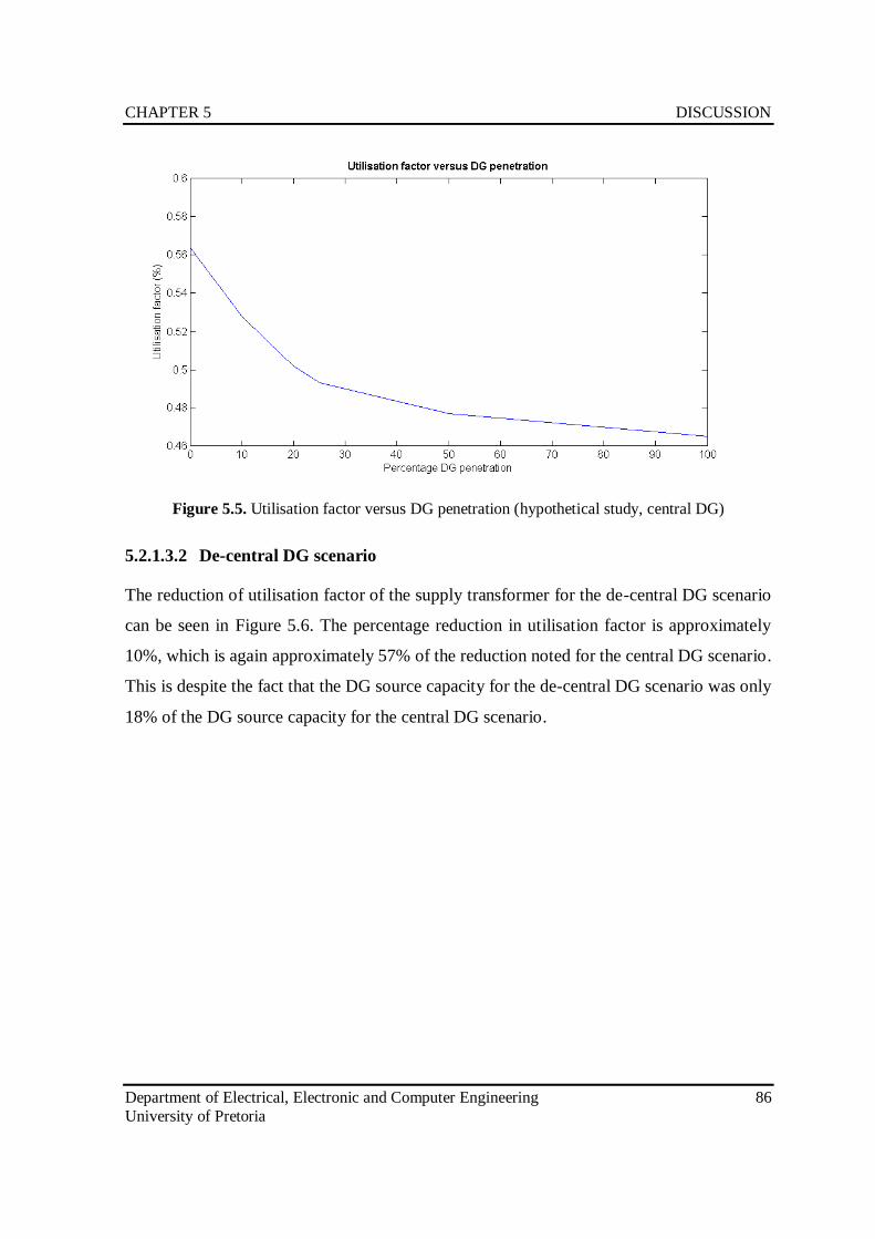
CHAPTER 5 DISCUSSION
Department of Electrical, Electronic and Computer Engineering 86
University of Pretoria
Figure 5.5. Utilisation factor versus DG penetration (hypothetical study, central DG)
5.2.1.3.2 De-central DG scenario
The reduction of utilisation factor of the supply transformer for the de-central DG scenario
can be seen in Figure 5.6. The percentage reduction in utilisation factor is approximately
10%, which is again approximately 57% of the reduction noted for the central DG scenario.
This is despite the fact that the DG source capacity for the de-central DG scenario was only
18% of the DG source capacity for the central DG scenario.
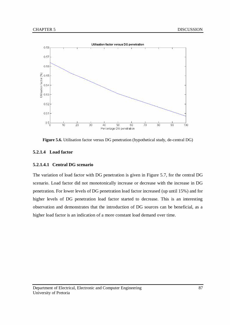
CHAPTER 5 DISCUSSION
Department of Electrical, Electronic and Computer Engineering 87
University of Pretoria
Figure 5.6. Utilisation factor versus DG penetration (hypothetical study, de-central DG)
5.2.1.4 Load factor
5.2.1.4.1 Central DG scenario
The variation of load factor with DG penetration is given in Figure 5.7, for the central DG
scenario. Load factor did not monotonically increase or decrease with the increase in DG
penetration. For lower levels of DG penetration load factor increased (up until 15%) and for
higher levels of DG penetration load factor started to decrease. This is an interesting
observation and demonstrates that the introduction of DG sources can be beneficial, as a
higher load factor is an indication of a more constant load demand over time.
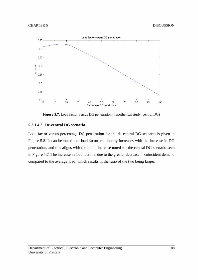
CHAPTER 5 DISCUSSION
Department of Electrical, Electronic and Computer Engineering 88
University of Pretoria
Figure 5.7. Load factor versus DG penetration (hypothetical study, central DG)
5.2.1.4.2 De-central DG scenario
Load factor versus percentage DG penetration for the de-central DG scenario is given in
Figure 5.8. It can be noted that load factor continually increases with the increase in DG
penetration, and this aligns with the initial increase noted for the central DG scenario seen
in Figure 5.7. The increase in load factor is due to the greater decrease in coincident demand
compared to the average load; which results in the ratio of the two being larger.
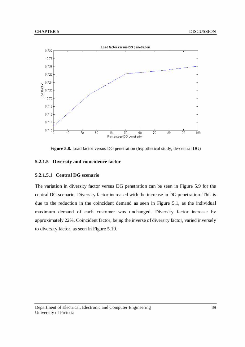
CHAPTER 5 DISCUSSION
Department of Electrical, Electronic and Computer Engineering 89
University of Pretoria
Figure 5.8. Load factor versus DG penetration (hypothetical study, de-central DG)
5.2.1.5 Diversity and coincidence factor
5.2.1.5.1 Central DG scenario
The variation in diversity factor versus DG penetration can be seen in Figure 5.9 for the
central DG scenario. Diversity factor increased with the increase in DG penetration. This is
due to the reduction in the coincident demand as seen in Figure 5.1, as the individual
maximum demand of each customer was unchanged. Diversity factor increase by
approximately 22%. Coincident factor, being the inverse of diversity factor, varied inversely
to diversity factor, as seen in Figure 5.10.
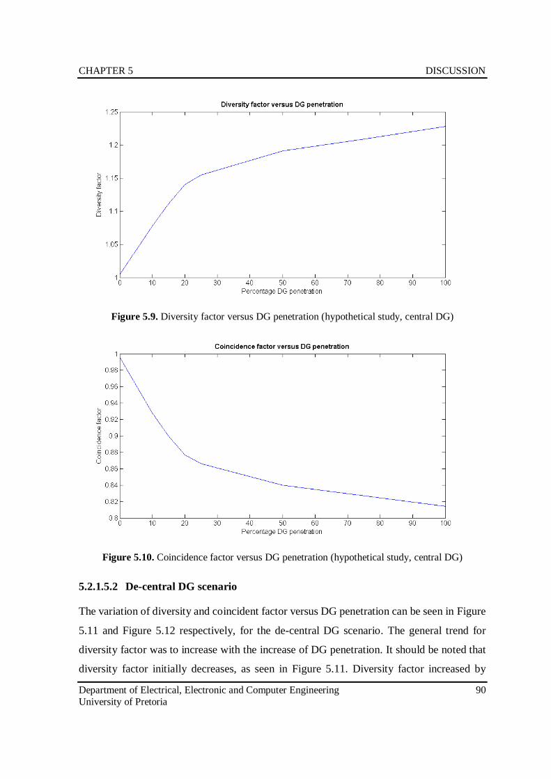
CHAPTER 5 DISCUSSION
Department of Electrical, Electronic and Computer Engineering 90
University of Pretoria
Figure 5.9. Diversity factor versus DG penetration (hypothetical study, central DG)
Figure 5.10. Coincidence factor versus DG penetration (hypothetical study, central DG)
5.2.1.5.2 De-central DG scenario
The variation of diversity and coincident factor versus DG penetration can be seen in Figure
5.11 and Figure 5.12 respectively, for the de-central DG scenario. The general trend for
diversity factor was to increase with the increase of DG penetration. It should be noted that
diversity factor initially decreases, as seen in Figure 5.11. Diversity factor increased by
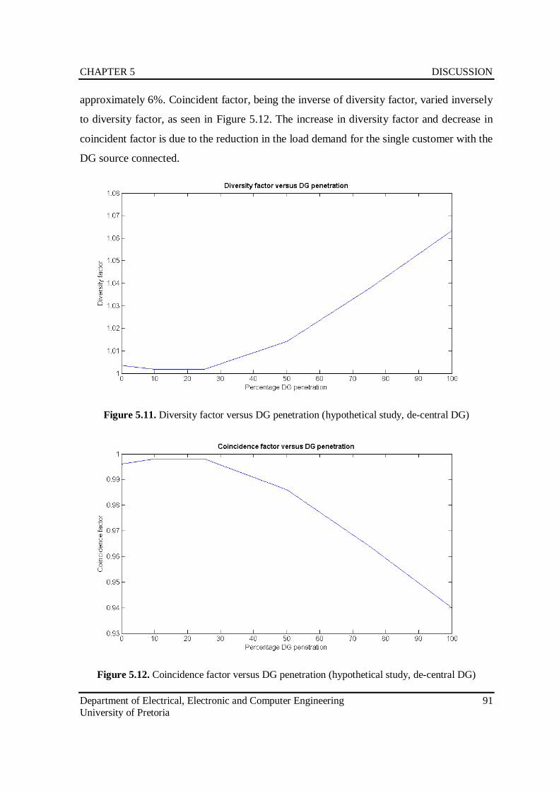
CHAPTER 5 DISCUSSION
Department of Electrical, Electronic and Computer Engineering 91
University of Pretoria
approximately 6%. Coincident factor, being the inverse of diversity factor, varied inversely
to diversity factor, as seen in Figure 5.12. The increase in diversity factor and decrease in
coincident factor is due to the reduction in the load demand for the single customer with the
DG source connected.
Figure 5.11. Diversity factor versus DG penetration (hypothetical study, de-central DG)
Figure 5.12. Coincidence factor versus DG penetration (hypothetical study, de-central DG)
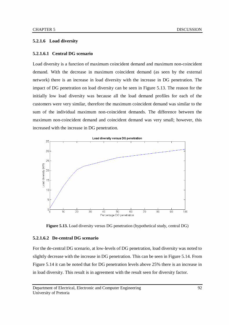
CHAPTER 5 DISCUSSION
Department of Electrical, Electronic and Computer Engineering 92
University of Pretoria
5.2.1.6 Load diversity
5.2.1.6.1 Central DG scenario
Load diversity is a function of maximum coincident demand and maximum non-coincident
demand. With the decrease in maximum coincident demand (as seen by the external
network) there is an increase in load diversity with the increase in DG penetration. The
impact of DG penetration on load diversity can be seen in Figure 5.13. The reason for the
initially low load diversity was because all the load demand profiles for each of the
customers were very similar, therefore the maximum coincident demand was similar to the
sum of the individual maximum non-coincident demands. The difference between the
maximum non-coincident demand and coincident demand was very small; however, this
increased with the increase in DG penetration.
Figure 5.13. Load diversity versus DG penetration (hypothetical study, central DG)
5.2.1.6.2 De-central DG scenario
For the de-central DG scenario, at low-levels of DG penetration, load diversity was noted to
slightly decrease with the increase in DG penetration. This can be seen in Figure 5.14. From
Figure 5.14 it can be noted that for DG penetration levels above 25% there is an increase in
in load diversity. This result is in agreement with the result seen for diversity factor.
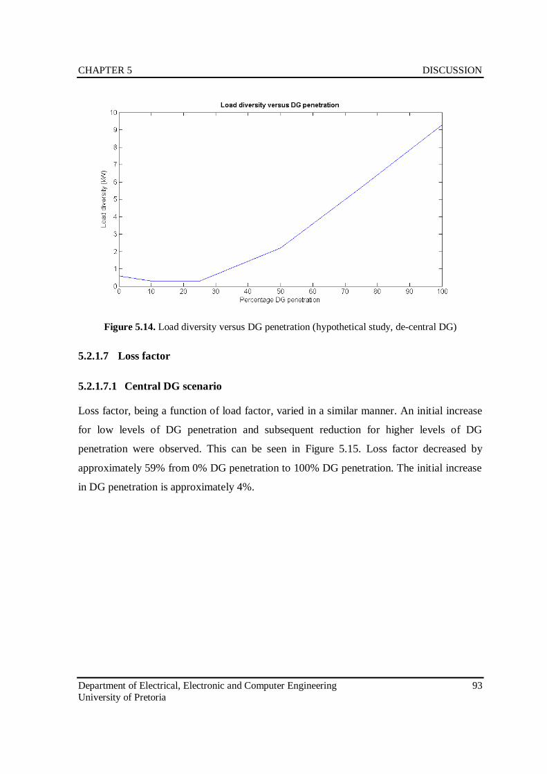
CHAPTER 5 DISCUSSION
Department of Electrical, Electronic and Computer Engineering 93
University of Pretoria
Figure 5.14. Load diversity versus DG penetration (hypothetical study, de-central DG)
5.2.1.7 Loss factor
5.2.1.7.1 Central DG scenario
Loss factor, being a function of load factor, varied in a similar manner. An initial increase
for low levels of DG penetration and subsequent reduction for higher levels of DG
penetration were observed. This can be seen in Figure 5.15. Loss factor decreased by
approximately 59% from 0% DG penetration to 100% DG penetration. The initial increase
in DG penetration is approximately 4%.
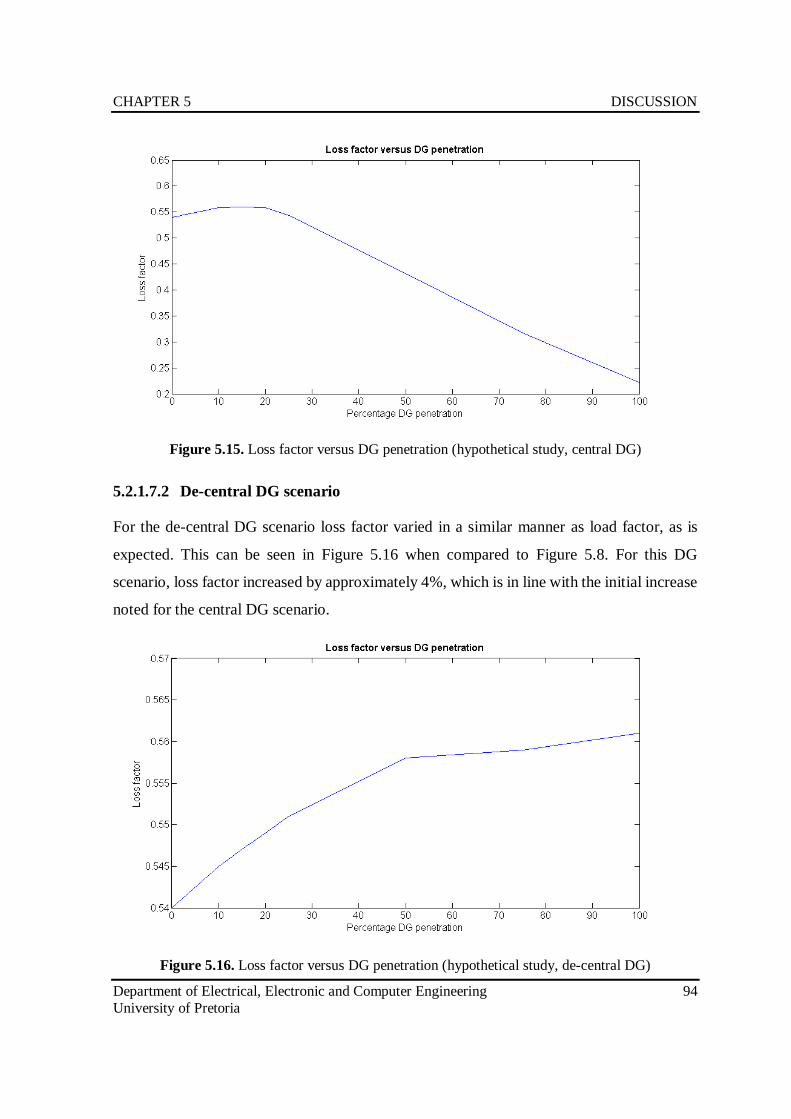
CHAPTER 5 DISCUSSION
Department of Electrical, Electronic and Computer Engineering 94
University of Pretoria
Figure 5.15. Loss factor versus DG penetration (hypothetical study, central DG)
5.2.1.7.2 De-central DG scenario
For the de-central DG scenario loss factor varied in a similar manner as load factor, as is
expected. This can be seen in Figure 5.16 when compared to Figure 5.8. For this DG
scenario, loss factor increased by approximately 4%, which is in line with the initial increase
noted for the central DG scenario.
Figure 5.16. Loss factor versus DG penetration (hypothetical study, de-central DG)
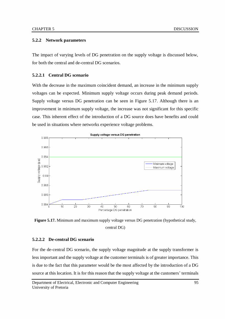
CHAPTER 5 DISCUSSION
Department of Electrical, Electronic and Computer Engineering 95
University of Pretoria
5.2.2 Network parameters
The impact of varying levels of DG penetration on the supply voltage is discussed below,
for both the central and de-central DG scenarios.
5.2.2.1 Central DG scenario
With the decrease in the maximum coincident demand, an increase in the minimum supply
voltages can be expected. Minimum supply voltage occurs during peak demand periods.
Supply voltage versus DG penetration can be seen in Figure 5.17. Although there is an
improvement in minimum supply voltage, the increase was not significant for this specific
case. This inherent effect of the introduction of a DG source does have benefits and could
be used in situations where networks experience voltage problems.
Figure 5.17. Minimum and maximum supply voltage versus DG penetration (hypothetical study,
central DG)
5.2.2.2 De-central DG scenario
For the de-central DG scenario, the supply voltage magnitude at the supply transformer is
less important and the supply voltage at the customer terminals is of greater importance. This
is due to the fact that this parameter would be the most affected by the introduction of a DG
source at this location. It is for this reason that the supply voltage at the customers’ terminals
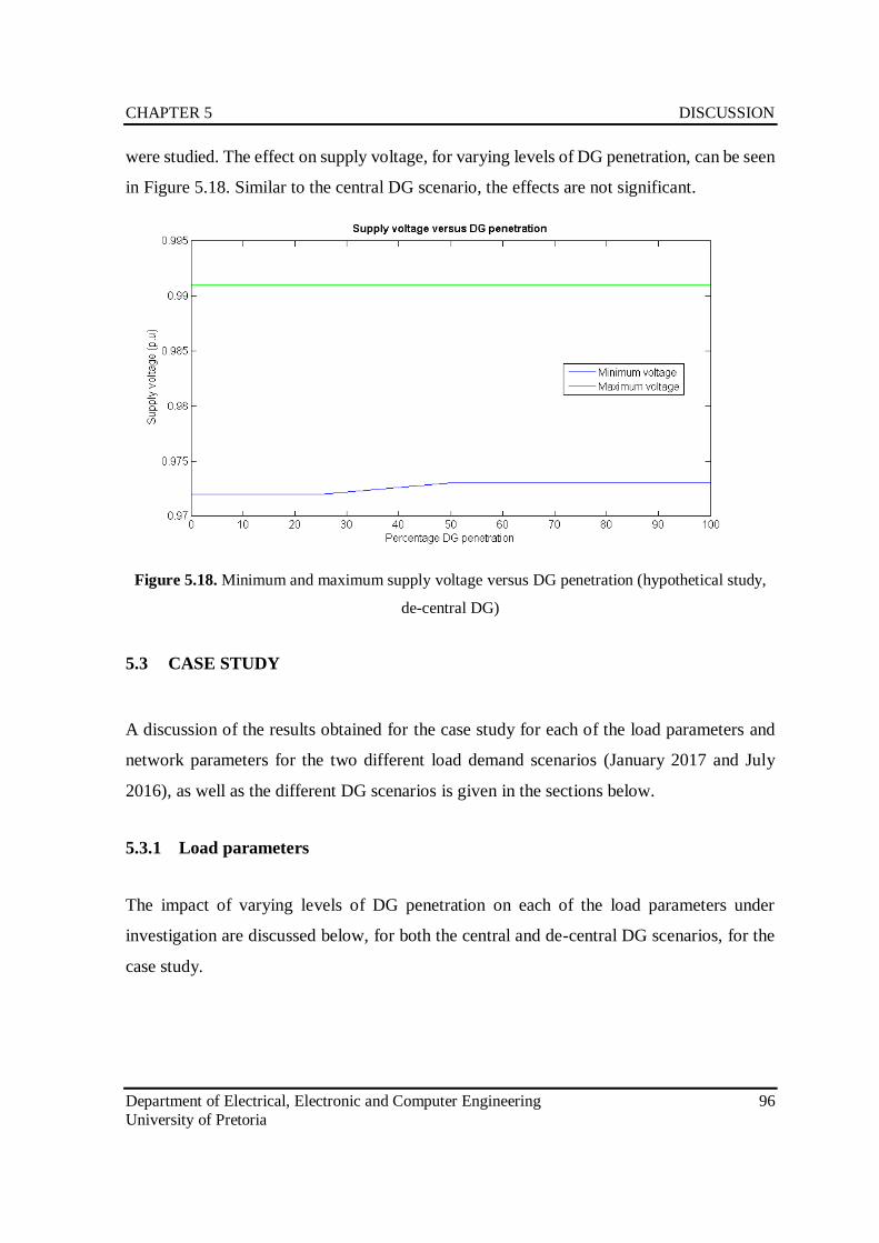
CHAPTER 5 DISCUSSION
Department of Electrical, Electronic and Computer Engineering 96
University of Pretoria
were studied. The effect on supply voltage, for varying levels of DG penetration, can be seen
in Figure 5.18. Similar to the central DG scenario, the effects are not significant.
Figure 5.18. Minimum and maximum supply voltage versus DG penetration (hypothetical study,
de-central DG)
5.3 CASE STUDY
A discussion of the results obtained for the case study for each of the load parameters and
network parameters for the two different load demand scenarios (January 2017 and July
2016), as well as the different DG scenarios is given in the sections below.
5.3.1 Load parameters
The impact of varying levels of DG penetration on each of the load parameters under
investigation are discussed below, for both the central and de-central DG scenarios, for the
case study.
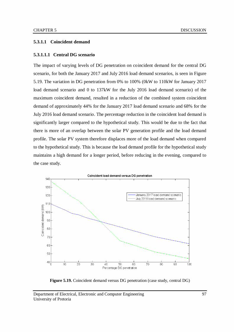
CHAPTER 5 DISCUSSION
Department of Electrical, Electronic and Computer Engineering 97
University of Pretoria
5.3.1.1 Coincident demand
5.3.1.1.1 Central DG scenario
The impact of varying levels of DG penetration on coincident demand for the central DG
scenario, for both the January 2017 and July 2016 load demand scenarios, is seen in Figure
5.19. The variation in DG penetration from 0% to 100% (0kW to 110kW for January 2017
load demand scenario and 0 to 137kW for the July 2016 load demand scenario) of the
maximum coincident demand, resulted in a reduction of the combined system coincident
demand of approximately 44% for the January 2017 load demand scenario and 68% for the
July 2016 load demand scenario. The percentage reduction in the coincident load demand is
significantly larger compared to the hypothetical study. This would be due to the fact that
there is more of an overlap between the solar PV generation profile and the load demand
profile. The solar PV system therefore displaces more of the load demand when compared
to the hypothetical study. This is because the load demand profile for the hypothetical study
maintains a high demand for a longer period, before reducing in the evening, compared to
the case study.
Figure 5.19. Coincident demand versus DG penetration (case study, central DG)
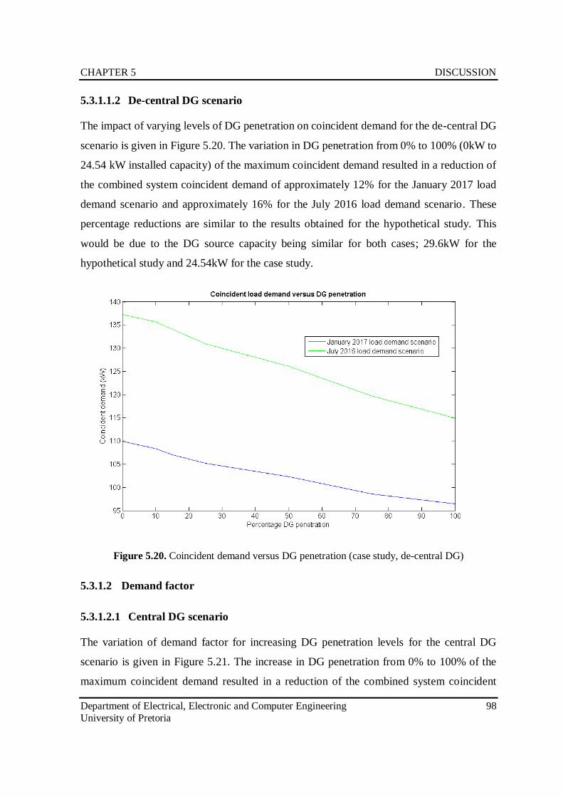
CHAPTER 5 DISCUSSION
Department of Electrical, Electronic and Computer Engineering 98
University of Pretoria
5.3.1.1.2 De-central DG scenario
The impact of varying levels of DG penetration on coincident demand for the de-central DG
scenario is given in Figure 5.20. The variation in DG penetration from 0% to 100% (0kW to
24.54 kW installed capacity) of the maximum coincident demand resulted in a reduction of
the combined system coincident demand of approximately 12% for the January 2017 load
demand scenario and approximately 16% for the July 2016 load demand scenario. These
percentage reductions are similar to the results obtained for the hypothetical study. This
would be due to the DG source capacity being similar for both cases; 29.6kW for the
hypothetical study and 24.54kW for the case study.
Figure 5.20. Coincident demand versus DG penetration (case study, de-central DG)
5.3.1.2 Demand factor
5.3.1.2.1 Central DG scenario
The variation of demand factor for increasing DG penetration levels for the central DG
scenario is given in Figure 5.21. The increase in DG penetration from 0% to 100% of the
maximum coincident demand resulted in a reduction of the combined system coincident
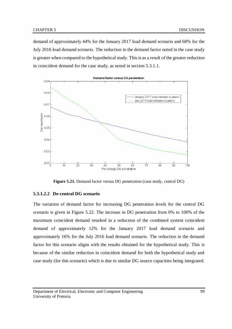
CHAPTER 5 DISCUSSION
Department of Electrical, Electronic and Computer Engineering 99
University of Pretoria
demand of approximately 44% for the January 2017 load demand scenario and 68% for the
July 2016 load demand scenario. The reduction in the demand factor noted in the case study
is greater when compared to the hypothetical study. This is as a result of the greater reduction
in coincident demand for the case study, as noted in section 5.3.1.1.
Figure 5.21. Demand factor versus DG penetration (case study, central DG)
5.3.1.2.2 De-central DG scenario
The variation of demand factor for increasing DG penetration levels for the central DG
scenario is given in Figure 5.22. The increase in DG penetration from 0% to 100% of the
maximum coincident demand resulted in a reduction of the combined system coincident
demand of approximately 12% for the January 2017 load demand scenario and
approximately 16% for the July 2016 load demand scenario. The reduction in the demand
factor for this scenario aligns with the results obtained for the hypothetical study. This is
because of the similar reduction in coincident demand for both the hypothetical study and
case study (for this scenario) which is due to similar DG source capacities being integrated.
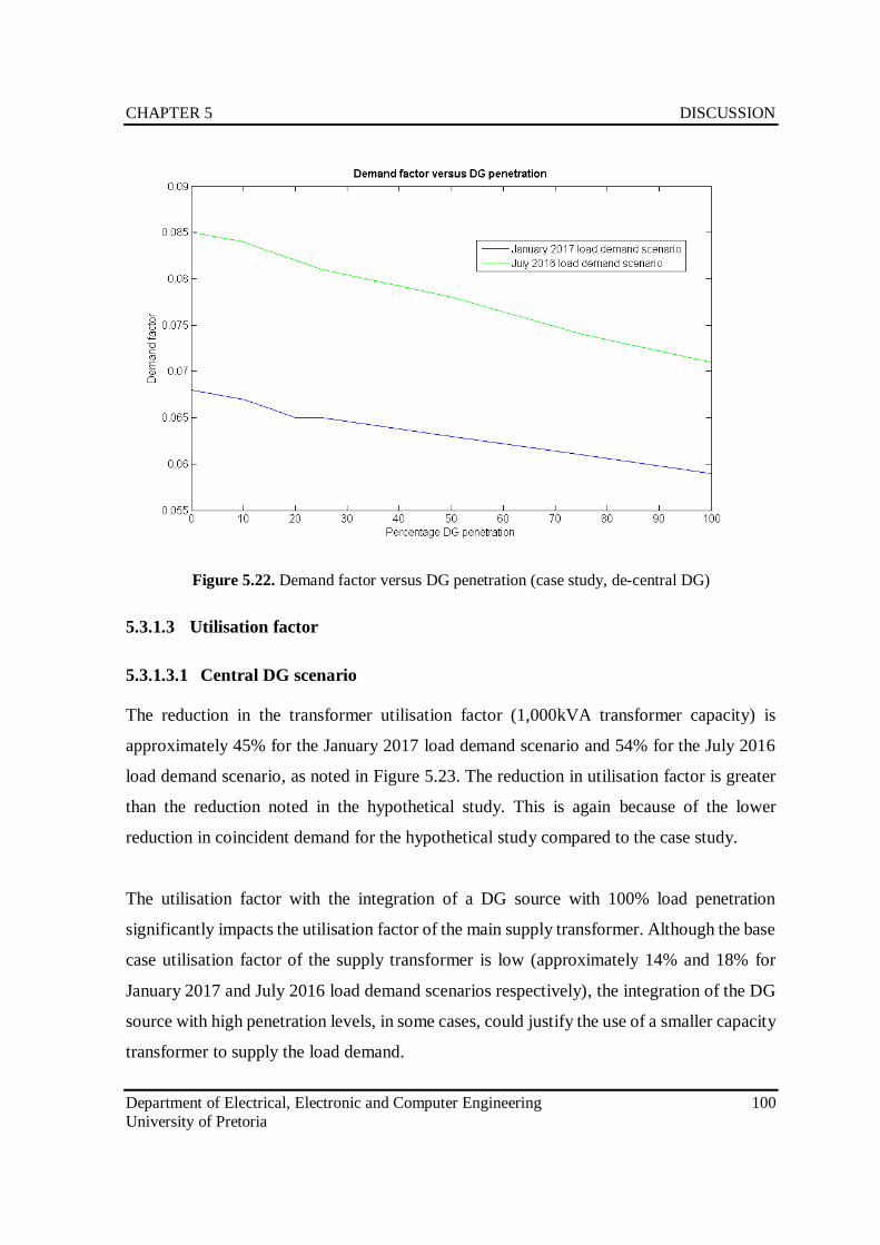
CHAPTER 5 DISCUSSION
Department of Electrical, Electronic and Computer Engineering 100
University of Pretoria
Figure 5.22. Demand factor versus DG penetration (case study, de-central DG)
5.3.1.3 Utilisation factor
5.3.1.3.1 Central DG scenario
The reduction in the transformer utilisation factor (1,000kVA transformer capacity) is
approximately 45% for the January 2017 load demand scenario and 54% for the July 2016
load demand scenario, as noted in Figure 5.23. The reduction in utilisation factor is greater
than the reduction noted in the hypothetical study. This is again because of the lower
reduction in coincident demand for the hypothetical study compared to the case study.
The utilisation factor with the integration of a DG source with 100% load penetration
significantly impacts the utilisation factor of the main supply transformer. Although the base
case utilisation factor of the supply transformer is low (approximately 14% and 18% for
January 2017 and July 2016 load demand scenarios respectively), the integration of the DG
source with high penetration levels, in some cases, could justify the use of a smaller capacity
transformer to supply the load demand.
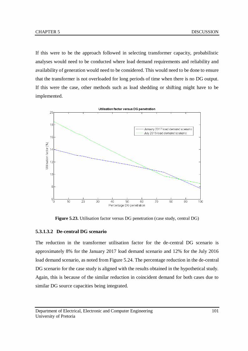
CHAPTER 5 DISCUSSION
Department of Electrical, Electronic and Computer Engineering 101
University of Pretoria
If this were to be the approach followed in selecting transformer capacity, probabilistic
analyses would need to be conducted where load demand requirements and reliability and
availability of generation would need to be considered. This would need to be done to ensure
that the transformer is not overloaded for long periods of time when there is no DG output.
If this were the case, other methods such as load shedding or shifting might have to be
implemented.
Figure 5.23. Utilisation factor versus DG penetration (case study, central DG)
5.3.1.3.2 De-central DG scenario
The reduction in the transformer utilisation factor for the de-central DG scenario is
approximately 8% for the January 2017 load demand scenario and 12% for the July 2016
load demand scenario, as noted from Figure 5.24. The percentage reduction in the de-central
DG scenario for the case study is aligned with the results obtained in the hypothetical study.
Again, this is because of the similar reduction in coincident demand for both cases due to
similar DG source capacities being integrated.
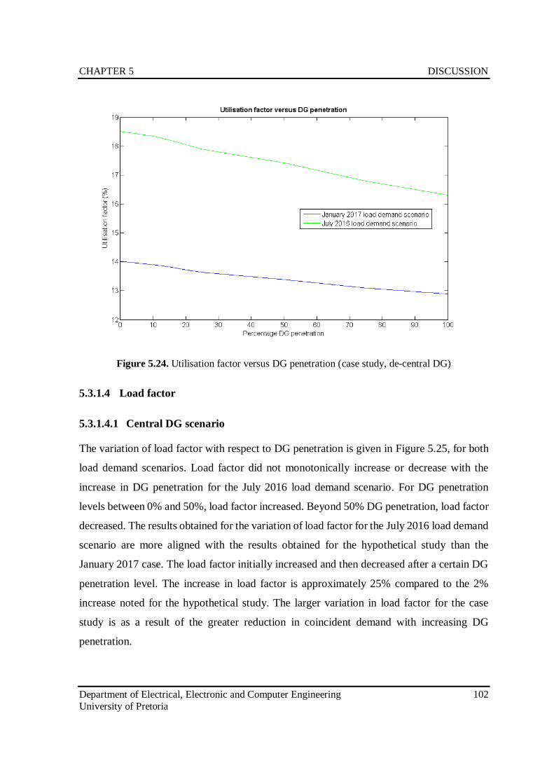
CHAPTER 5 DISCUSSION
Department of Electrical, Electronic and Computer Engineering 102
University of Pretoria
Figure 5.24. Utilisation factor versus DG penetration (case study, de-central DG)
5.3.1.4 Load factor
5.3.1.4.1 Central DG scenario
The variation of load factor with respect to DG penetration is given in Figure 5.25, for both
load demand scenarios. Load factor did not monotonically increase or decrease with the
increase in DG penetration for the July 2016 load demand scenario. For DG penetration
levels between 0% and 50%, load factor increased. Beyond 50% DG penetration, load factor
decreased. The results obtained for the variation of load factor for the July 2016 load demand
scenario are more aligned with the results obtained for the hypothetical study than the
January 2017 case. The load factor initially increased and then decreased after a certain DG
penetration level. The increase in load factor is approximately 25% compared to the 2%
increase noted for the hypothetical study. The larger variation in load factor for the case
study is as a result of the greater reduction in coincident demand with increasing DG
penetration.
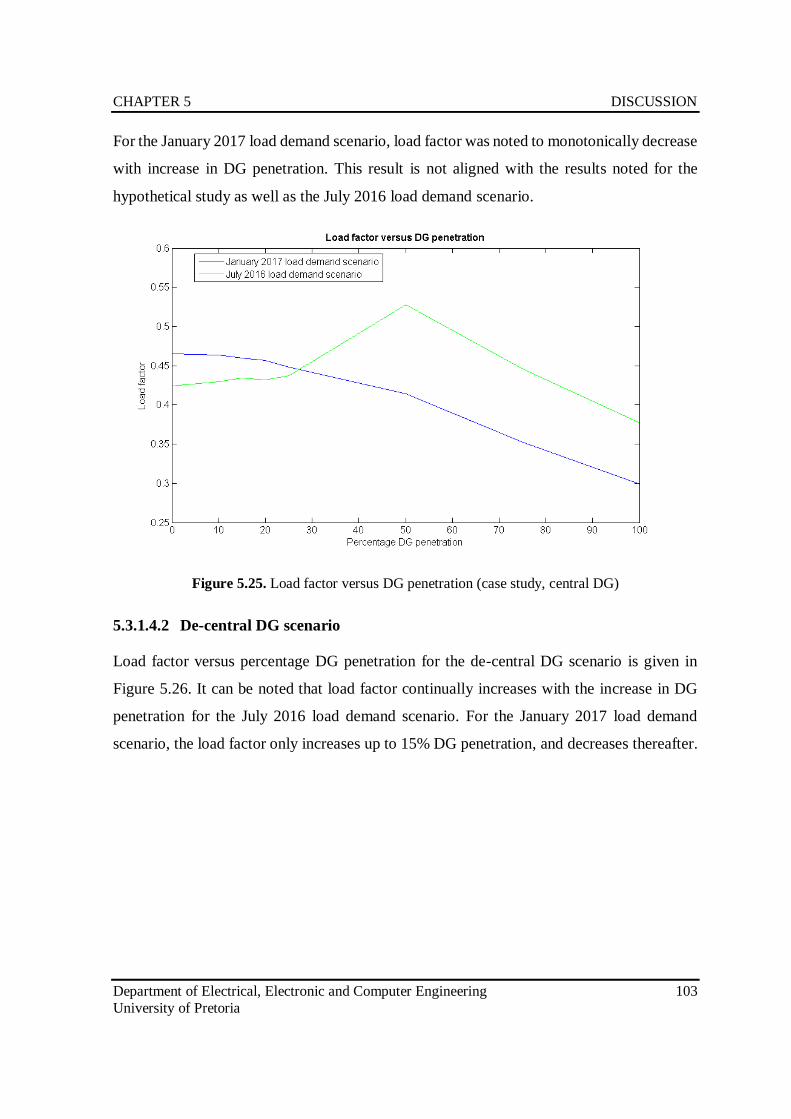
CHAPTER 5 DISCUSSION
Department of Electrical, Electronic and Computer Engineering 103
University of Pretoria
For the January 2017 load demand scenario, load factor was noted to monotonically decrease
with increase in DG penetration. This result is not aligned with the results noted for the
hypothetical study as well as the July 2016 load demand scenario.
Figure 5.25. Load factor versus DG penetration (case study, central DG)
5.3.1.4.2 De-central DG scenario
Load factor versus percentage DG penetration for the de-central DG scenario is given in
Figure 5.26. It can be noted that load factor continually increases with the increase in DG
penetration for the July 2016 load demand scenario. For the January 2017 load demand
scenario, the load factor only increases up to 15% DG penetration, and decreases thereafter.
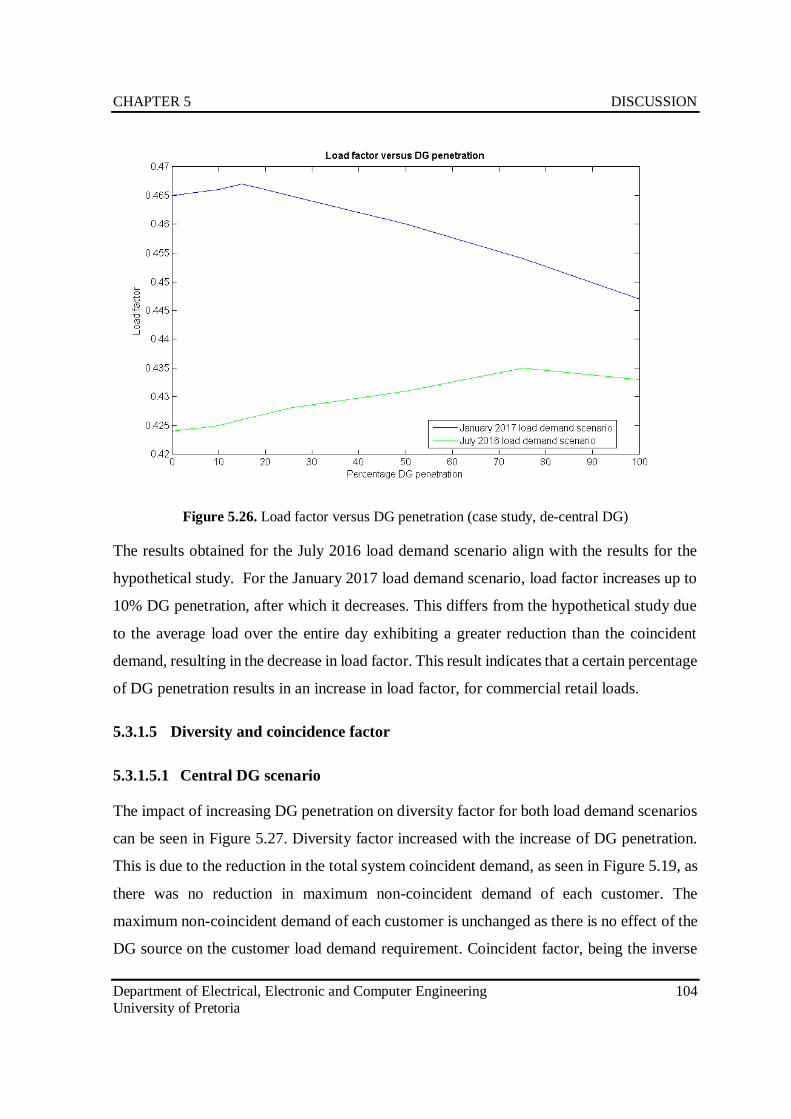
CHAPTER 5 DISCUSSION
Department of Electrical, Electronic and Computer Engineering 104
University of Pretoria
Figure 5.26. Load factor versus DG penetration (case study, de-central DG)
The results obtained for the July 2016 load demand scenario align with the results for the
hypothetical study. For the January 2017 load demand scenario, load factor increases up to
10% DG penetration, after which it decreases. This differs from the hypothetical study due
to the average load over the entire day exhibiting a greater reduction than the coincident
demand, resulting in the decrease in load factor. This result indicates that a certain percentage
of DG penetration results in an increase in load factor, for commercial retail loads.
5.3.1.5 Diversity and coincidence factor
5.3.1.5.1 Central DG scenario
The impact of increasing DG penetration on diversity factor for both load demand scenarios
can be seen in Figure 5.27. Diversity factor increased with the increase of DG penetration.
This is due to the reduction in the total system coincident demand, as seen in Figure 5.19, as
there was no reduction in maximum non-coincident demand of each customer. The
maximum non-coincident demand of each customer is unchanged as there is no effect of the
DG source on the customer load demand requirement. Coincident factor, being the inverse
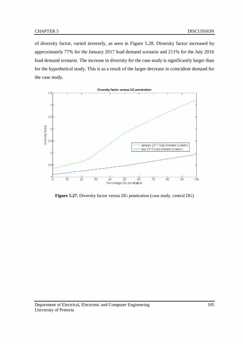
CHAPTER 5 DISCUSSION
Department of Electrical, Electronic and Computer Engineering 105
University of Pretoria
of diversity factor, varied inversely, as seen in Figure 5.28. Diversity factor increased by
approximately 77% for the January 2017 load demand scenario and 211% for the July 2016
load demand scenario. The increase in diversity for the case study is significantly larger than
for the hypothetical study. This is as a result of the larger decrease in coincident demand for
the case study.
Figure 5.27. Diversity factor versus DG penetration (case study, central DG)
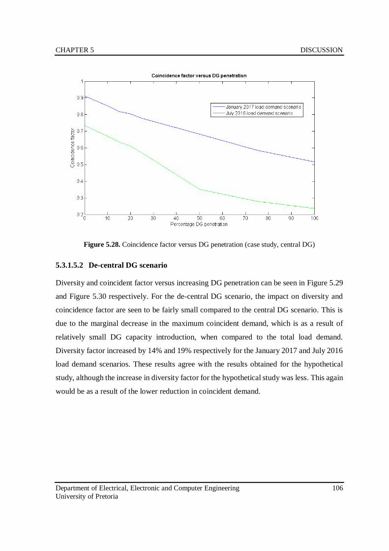
CHAPTER 5 DISCUSSION
Department of Electrical, Electronic and Computer Engineering 106
University of Pretoria
Figure 5.28. Coincidence factor versus DG penetration (case study, central DG)
5.3.1.5.2 De-central DG scenario
Diversity and coincident factor versus increasing DG penetration can be seen in Figure 5.29
and Figure 5.30 respectively. For the de-central DG scenario, the impact on diversity and
coincidence factor are seen to be fairly small compared to the central DG scenario. This is
due to the marginal decrease in the maximum coincident demand, which is as a result of
relatively small DG capacity introduction, when compared to the total load demand.
Diversity factor increased by 14% and 19% respectively for the January 2017 and July 2016
load demand scenarios. These results agree with the results obtained for the hypothetical
study, although the increase in diversity factor for the hypothetical study was less. This again
would be as a result of the lower reduction in coincident demand.
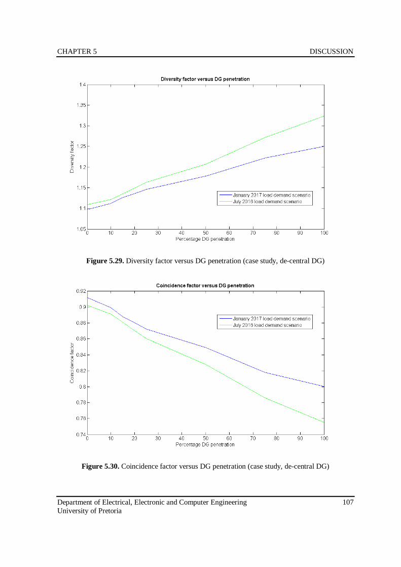
CHAPTER 5 DISCUSSION
Department of Electrical, Electronic and Computer Engineering 107
University of Pretoria
Figure 5.29. Diversity factor versus DG penetration (case study, de-central DG)
Figure 5.30. Coincidence factor versus DG penetration (case study, de-central DG)
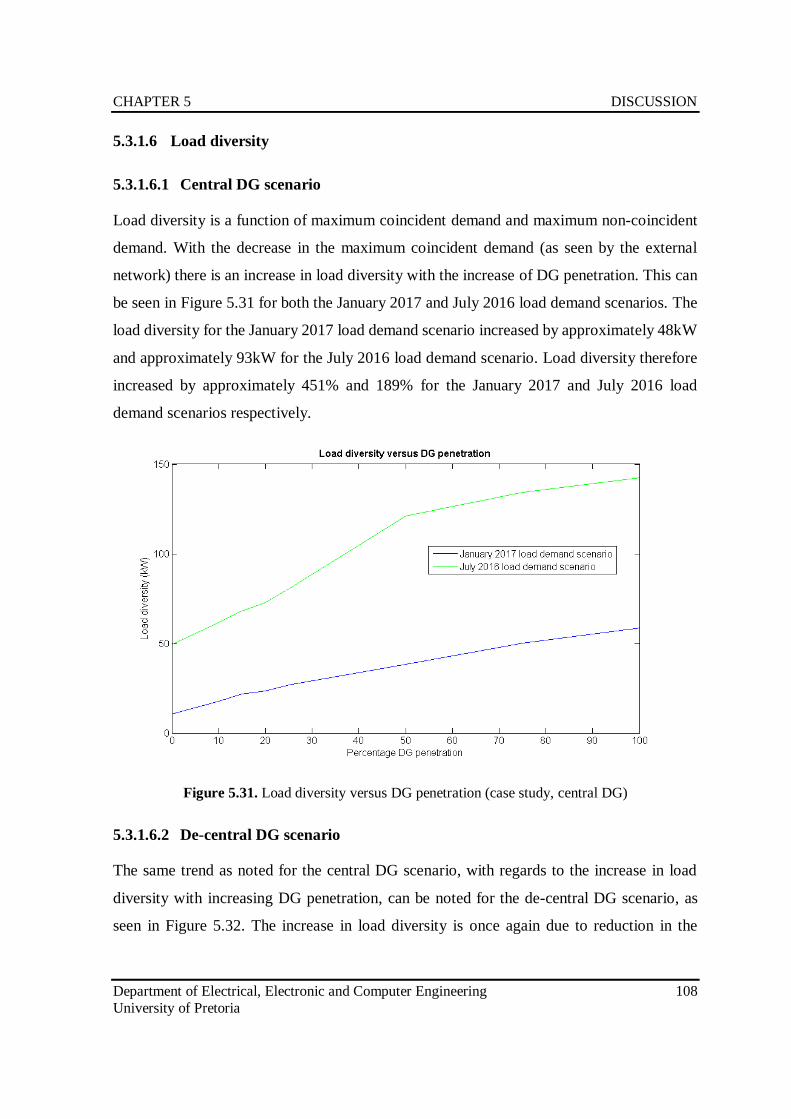
CHAPTER 5 DISCUSSION
Department of Electrical, Electronic and Computer Engineering 108
University of Pretoria
5.3.1.6 Load diversity
5.3.1.6.1 Central DG scenario
Load diversity is a function of maximum coincident demand and maximum non-coincident
demand. With the decrease in the maximum coincident demand (as seen by the external
network) there is an increase in load diversity with the increase of DG penetration. This can
be seen in Figure 5.31 for both the January 2017 and July 2016 load demand scenarios. The
load diversity for the January 2017 load demand scenario increased by approximately 48kW
and approximately 93kW for the July 2016 load demand scenario. Load diversity therefore
increased by approximately 451% and 189% for the January 2017 and July 2016 load
demand scenarios respectively.
Figure 5.31. Load diversity versus DG penetration (case study, central DG)
5.3.1.6.2 De-central DG scenario
The same trend as noted for the central DG scenario, with regards to the increase in load
diversity with increasing DG penetration, can be noted for the de-central DG scenario, as
seen in Figure 5.32. The increase in load diversity is once again due to reduction in the
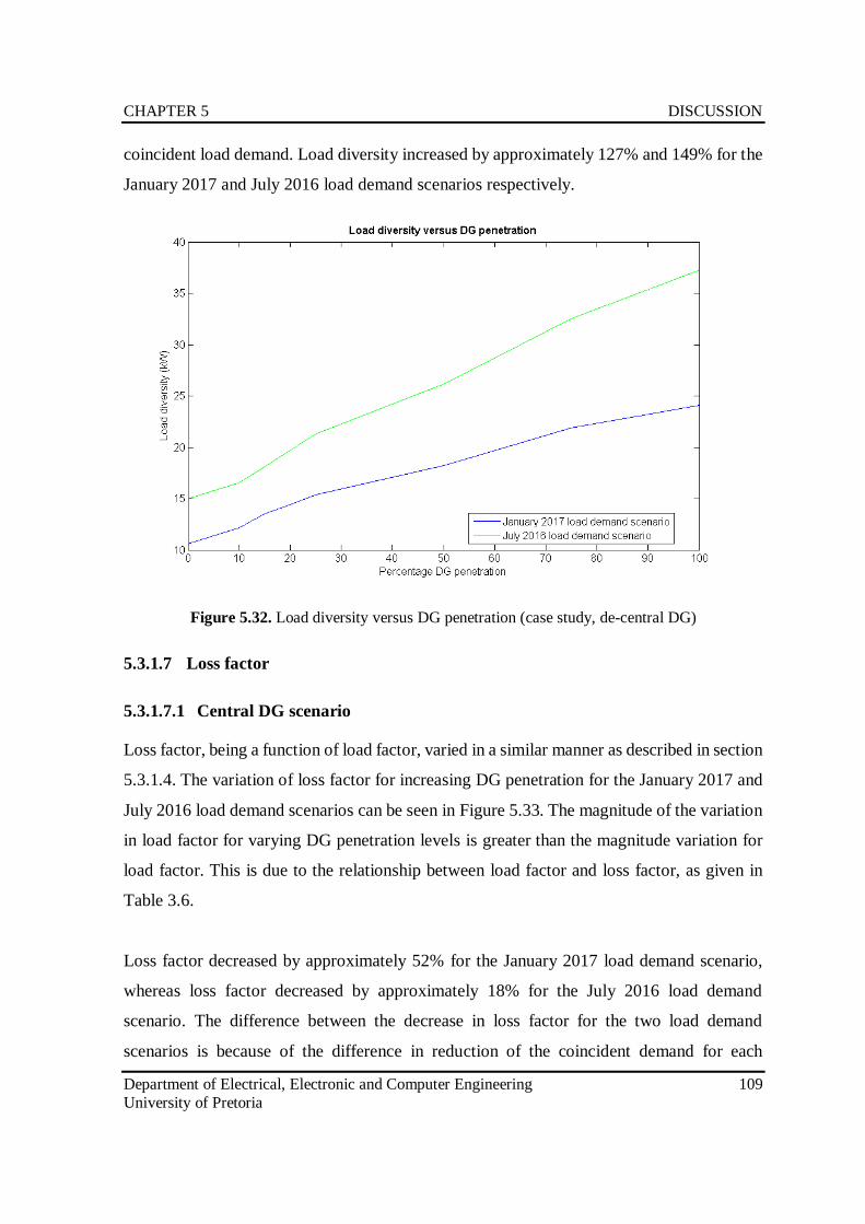
CHAPTER 5 DISCUSSION
Department of Electrical, Electronic and Computer Engineering 109
University of Pretoria
coincident load demand. Load diversity increased by approximately 127% and 149% for the
January 2017 and July 2016 load demand scenarios respectively.
Figure 5.32. Load diversity versus DG penetration (case study, de-central DG)
5.3.1.7 Loss factor
5.3.1.7.1 Central DG scenario
Loss factor, being a function of load factor, varied in a similar manner as described in section
5.3.1.4. The variation of loss factor for increasing DG penetration for the January 2017 and
July 2016 load demand scenarios can be seen in Figure 5.33. The magnitude of the variation
in load factor for varying DG penetration levels is greater than the magnitude variation for
load factor. This is due to the relationship between load factor and loss factor, as given in
Table 3.6.
Loss factor decreased by approximately 52% for the January 2017 load demand scenario,
whereas loss factor decreased by approximately 18% for the July 2016 load demand
scenario. The difference between the decrease in loss factor for the two load demand
scenarios is because of the difference in reduction of the coincident demand for each
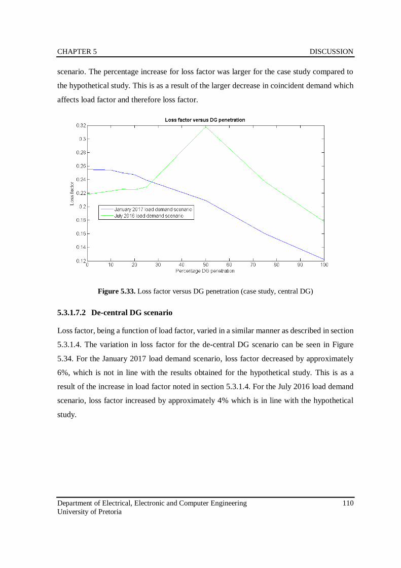
CHAPTER 5 DISCUSSION
Department of Electrical, Electronic and Computer Engineering 110
University of Pretoria
scenario. The percentage increase for loss factor was larger for the case study compared to
the hypothetical study. This is as a result of the larger decrease in coincident demand which
affects load factor and therefore loss factor.
Figure 5.33. Loss factor versus DG penetration (case study, central DG)
5.3.1.7.2 De-central DG scenario
Loss factor, being a function of load factor, varied in a similar manner as described in section
5.3.1.4. The variation in loss factor for the de-central DG scenario can be seen in Figure
5.34. For the January 2017 load demand scenario, loss factor decreased by approximately
6%, which is not in line with the results obtained for the hypothetical study. This is as a
result of the increase in load factor noted in section 5.3.1.4. For the July 2016 load demand
scenario, loss factor increased by approximately 4% which is in line with the hypothetical
study.
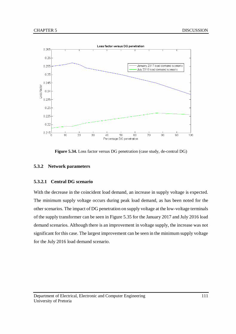
CHAPTER 5 DISCUSSION
Department of Electrical, Electronic and Computer Engineering 111
University of Pretoria
Figure 5.34. Loss factor versus DG penetration (case study, de-central DG)
5.3.2 Network parameters
5.3.2.1 Central DG scenario
With the decrease in the coincident load demand, an increase in supply voltage is expected.
The minimum supply voltage occurs during peak load demand, as has been noted for the
other scenarios. The impact of DG penetration on supply voltage at the low-voltage terminals
of the supply transformer can be seen in Figure 5.35 for the January 2017 and July 2016 load
demand scenarios. Although there is an improvement in voltage supply, the increase was not
significant for this case. The largest improvement can be seen in the minimum supply voltage
for the July 2016 load demand scenario.
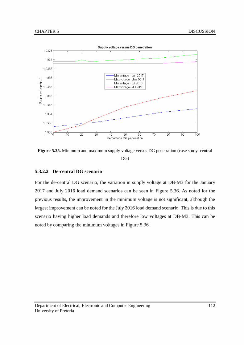
CHAPTER 5 DISCUSSION
Department of Electrical, Electronic and Computer Engineering 112
University of Pretoria
Figure 5.35. Minimum and maximum supply voltage versus DG penetration (case study, central
DG)
5.3.2.2 De-central DG scenario
For the de-central DG scenario, the variation in supply voltage at DB-M3 for the January
2017 and July 2016 load demand scenarios can be seen in Figure 5.36. As noted for the
previous results, the improvement in the minimum voltage is not significant, although the
largest improvement can be noted for the July 2016 load demand scenario. This is due to this
scenario having higher load demands and therefore low voltages at DB-M3. This can be
noted by comparing the minimum voltages in Figure 5.36.
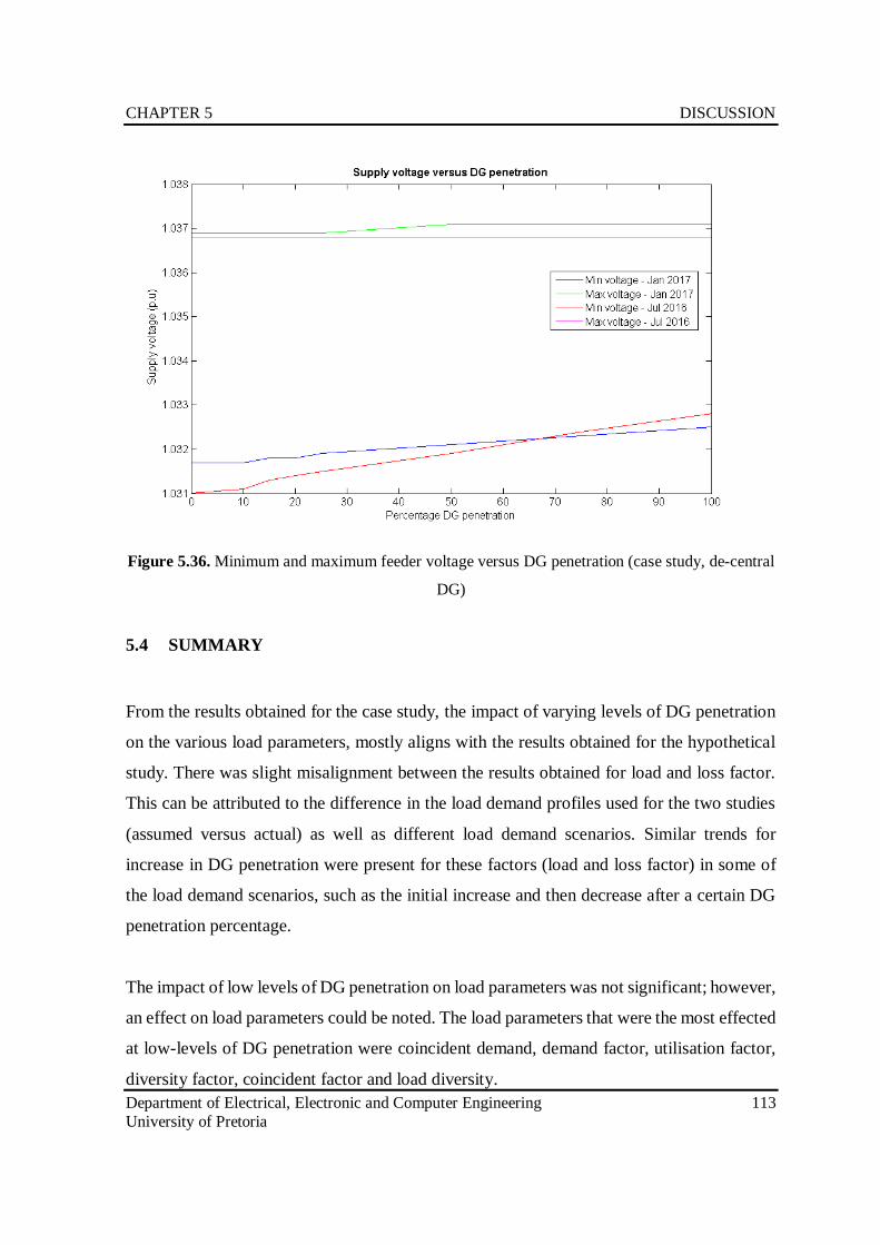
CHAPTER 5 DISCUSSION
Department of Electrical, Electronic and Computer Engineering 113
University of Pretoria
Figure 5.36. Minimum and maximum feeder voltage versus DG penetration (case study, de-central
DG)
5.4 SUMMARY
From the results obtained for the case study, the impact of varying levels of DG penetration
on the various load parameters, mostly aligns with the results obtained for the hypothetical
study. There was slight misalignment between the results obtained for load and loss factor.
This can be attributed to the difference in the load demand profiles used for the two studies
(assumed versus actual) as well as different load demand scenarios. Similar trends for
increase in DG penetration were present for these factors (load and loss factor) in some of
the load demand scenarios, such as the initial increase and then decrease after a certain DG
penetration percentage.
The impact of low levels of DG penetration on load parameters was not significant; however,
an effect on load parameters could be noted. The load parameters that were the most effected
at low-levels of DG penetration were coincident demand, demand factor, utilisation factor,
diversity factor, coincident factor and load diversity.
CHAPTER 5 DISCUSSION
Department of Electrical, Electronic and Computer Engineering 114
University of Pretoria
These are all parameters that are related to coincident demand. Factors such as load factor
and loss factor were only marginally affected at low DG penetration levels. Load and loss
factor were most significantly affected at high DG penetration levels. All load parameters
were, however, significantly impacted at high DG penetration levels.
The most noticeable impact on load parameters was seen in the central DG scenario. This is
due to the large DG system capacity integrated, which affects coincident demand more
significantly when compared to the de-central DG scenario. The load demand profile is
therefore impacted significantly (for the central DG scenario) and results in the greatest
variation in load parameters. A variation in load parameters was noted for the de-central DG
scenario; however, due to the smaller installed system capacities the effect was not as large
as for the central DG scenario.
Network parameters such as supply voltage were only slightly improved at high DG
penetration levels. Although only slightly impacted, the effect of increasing DG penetration
to improve supply voltage could be noted and is beneficial to networks that experience
voltage problems, such as under-voltage. This effect could not be accurately modelled as
information or data pertaining to supply voltage within the network or upstream network
information was unavailable for the study.
CHAPTER 6 CONCLUSION
With the worldwide focus on becoming more sustainable and environmentally conscious,
the uptake of renewable energy DG sources is increasing. The studies conducted in this
research topic have proven that introducing DG in low-voltage networks, such as
commercial retail reticulation networks, does affect the load parameters. It is therefore
imperative to understand what the effects of integrating DG is on load parameters, to ensure
that future network planning and design is done successfully, safely and effectively. As one
of the key input parameters into network planning and network design is the load parameters,
for which the network should service.
Commercial retail reticulation networks typically form part of a larger power system.
Understanding how load parameters are altered from the introduction of DG aids in
successful and efficient network planning and design that is done at a distribution, sub-
transmission or even transmission power system level. The knowledge gained by
understanding how the load parameters are affected by the introduction of DG can ensure
that future load forecasting is done accurately.
Determining the effect of DG on load parameters such as coincident demand, utilisation
factor, load factor, diversity factor, load diversity and loss factor is important and was
determined by the study. Understanding how these load parameters are altered from the
integration of DG provides insight to assist in planning and design of reticulation networks,
to service commercial retail customers that contain varying levels of DG penetration.
When integrating DG into reticulation networks there are many technical issues that need to
be considered. Two such examples are ensuring that the thermal rating of equipment is not
CHAPTER 6 CONCLUSION
Department of Electrical, Electronic and Computer Engineering 116
University of Pretoria
exceeded and voltage rise is limited to within specific tolerances. These issues did not occur
in this study.
The variation between the base case load parameters (no DG present) and altered load
parameters for varying levels of DG penetration were analysed, and based on solar PV DG
source. It can be seen from the results that the introduction of DG into a commercial retail
network can significantly alter load parameters of the composite load, as seen by the external
network, at high penetration levels. Load parameters were found to be altered from the
introduction of DG and varied as a function of DG penetration.
The load parameters which decreased with an increase in DG penetration were coincident
demand, demand factor, utilisation factor and coincidence factor, for both the central DG
scenario and de-central DG scenario. Load parameters which were noted to increase with
the increase in DG penetration were diversity factor and load diversity. Load and loss factor
(loss factor being a function of load factor) was not monotonic, as was noted for the other
load parameters.
In both DG scenarios (central and de-central) load and loss factor were noted to initially
increase with DG penetration until a certain percentage penetration, thereafter a decrease
was noted. The load and loss factor parameters for the January 2017 load demand scenario,
for the case study, did not exhibit such behaviour. These parameters were noted to
continually decrease with the increase in DG penetration. This is as result of a greater
decrease in average load compared to the coincident demand. For this demand scenario, a
solar PV DG system does not have the ability to reduce the maximum coincident demand
that occurs later in the day due to reduced generation output in the late afternoon or evening.
The results obtained are also in agreement with the hypothesised results and confirmed by
both the hypothetical study and the case study, based on actual load demand data and
reticulation network information.
CHAPTER 6 CONCLUSION
Department of Electrical, Electronic and Computer Engineering 117
University of Pretoria
The overlap between the load demand profile and DG source generation profile plays an
important role in determining how the different load parameters are effected. The greater the
overlap, the great the impact will be. A typical commercial load demand profile coincides
with a solar PV DG source. At high penetration levels, load parameters are therefore
significantly affected. As the load demand profile and generation profile of the DG source
play an important role in the analysis, any changes to one of the two would result in different
effects on load parameters. To accurately determine the effect of varying levels of DG
penetration on load parameters would require a case by case analysis.
Coincident demand, diversity factor and load factor play an important role in the design of
reticulation networks suitable to supply the relevant load demand requirements. The results
obtained indicate that there is a need to re-assess the suitability of existing planning and
design procedures or standards for reticulation networks due to the altering of load and
network parameters from the introduction of DG sources to commercial retail reticulation
networks.
REFERENCES
[1] T. Ackermann, G. Andersson and L. Sober, “Distributed generation: a definition,”
Electric Power Systems Research, vol. 57, no. 3, pp. 195-204, Apr. 2001.
[2] U. Minnaar, “Regulatory practices and Distribution System Cost impact studies for
distributed generation: Considerations for South African distribution utilities and
regulators,” Renewable and Sustainable Energy Reviews, vol. 56, pp. 1139-1149,
2016.
[3] M. Mahmud, M. Hossain and H. Pota, “Analysis of Voltage Rise Effect on
Distribution Network with Distributed Generation,” in 18th IFAC World Congress,
Milano (Italy), pp 14796-14801, 2011.
[4] A. Keane and M. O'Malley, “Impact of Distributed Generation Capacity and Losses,”
in Proc. IEEE PES General Meeting, Montreal (Canada), pp 54-58, 2006.
[5] J. Alberts and J. de Kock, “The Impact of Small Scale Embedded Generation and
EEDSM on historically designed networks and how it will affect networks of future
cities,” in 64th AMEU Convention, Johannesburg, pp 1-7, 2014
[6] I. Davidson, “Modeling and Analysis of a Multi-Bus Reticulation Network with
Multiple DG (Part I - Electrical Losses),” in IEEE Africon , Botswana, pp 805-810,
2004
[7] G. Moodley, G. Jennings and V. Pillay, “Typical technical behaviour of LV networks
with varied levels of renewable penetration,” in 64th AMEU Convention ,
Johannesburg, pp 62-64, 2014.
REFERENCES
Department of Electrical, Electronic and Computer Engineering 119
University of Pretoria
[8] S. Abdi and K. Afshar, “Application of IPSO-Monte Carlo for optimal distributed
generation allocation,” Electrical Power & Energy Systems , vol. 44, pp. 786-797,
2013.
[9] M. Aman, G. Jasmon and A. M. H. Bakar, “A new approach for optimum DG
placement and sizing based on voltage stability maximization and minization of
power losses,” Energy Conversion and Management, vol. 70, pp. 202-210, 2013.
[10] S. Devi and Geethanjali, “Optimal location and sizing determination of distributed
generation and DTATCOM using Partical Swarm Optimization algorithm,”
International Journal of Electrical Power & Energy Systems, vol. 62, pp. 562-570,
2014.
[11] A. EL-Zonkoly, “Optimal placement of multi-distributed generation units including
different load models using particle swarm optimisation,” IET Generation,
Transmission & Distribution , vol. 5, no. 7, pp. 760-771, 2011.
[12] S. Kansal, V. Kumar and B. Tyagi, “Optimal placement of different types of DG
sources in distribution networks,” Electrical Power and Energy Systems , no. 53, pp.
752-760, 2013.
[13] M. Moradi and M. Abedini, “A combination of genetic algorithm and particle swarm
optimization for optimal DG location and sizing in distribution systems,”
International Journal of Electrical Power & Energy Systems, vol. 34, no. 1, pp. 66-
74, 2012.
[14] A. Zelinalzadeh, Y. Mohammadi and M. Moradi, “Optimal multi objective
placement and sizing of multiple DGs and shunt capacitor banks simultaneously
considering load uncertainty via MOPSO approach,” International Jounal of
Electrical Power & Energy Systems , vol. 67, pp. 336-349, 2015.
[15] P. Barker and R. de Mello, “Determining the Impact of Distributed Generation on
Power Systems: Part 1 - Radial Distribution Systems,” IEEE Transaction on Power
Delivery , vol. 15, pp. 486-493, 2000.
REFERENCES
Department of Electrical, Electronic and Computer Engineering 120
University of Pretoria
[16] S. Brahma and A. Girgis, “Development of adaptive protection scheme for
distribution systems with high penetration of distributed generation,” IEEE
Transactions on Power Delivery , vol. 19, no. 1, pp. 56-63, 2004.
[17] A. Fazanehrafat, S. B. S. Javadian and M. Haghifamt, “Maintaining The Recloser-
Fuse Coordination in Distribution Systems in Presence of DG by Determining DG's
Size,” in Developments in Power System Protection, 2008. DPSP 2008. IET 9th
International Conference on, Glasgow, pp 132-137, 2008.
[18] K. Kauhaniemi and L. Kumpulainen, “Impact of distributed generation on the
protection of distributed networks,” in Developments in Power System Protection,
Amsterdam, pp 315-318, 2004.
[19] P. Manditereza and R. Bansal, “Renewable distributed generation: The hidden
chanllenges - A review from the protection perspective,” Renewable and Sustainable
Energy Reviews, vol. 58, pp. 1457-1465, 2016.
[20] D. Martin, P. Sharma, A. Sinclair and D. Finney, “Distance protection in distribution
systems: How it assists with integrating distributed resources,” in 65th Annual
Conference for Protective Relay Engineers, Texas, pp 166-177, 2012.
[21] S. Shahriari, M. Abapour, A. Yazdian and M. Haghifam, “Minimizing the impact of
Distributed Generation on Distribution Protection System by Solid State Fault
Current Limiter,” in Transmission and Distribution Conference and Exposition, New
Orleans, pp 1-7, 2010.
[22] International Energy Agency, “Energy Technology Perspectives,” International
Energy Agency, France, 2010.
[23] Berkeley Lab, “Microgrids at Berkeley Lab,” U.S Department of Energy, 2016.
[Online]. Available: https://building-microgrid.lbl.gov/microgrid-definitions.
[Accessed 30 03 2016].
REFERENCES
Department of Electrical, Electronic and Computer Engineering 121
University of Pretoria
[24] C. Masters, “Voltage rise the big issue when connecting embedded generation to long
11kV overhead lines,” Power Engineering Journal, vol. 16, pp. 5-12, 2002.
[25] A. Jordehi, “Allocation of distributed generation units in electric power systems: A
review,” Renewable and Sustainable Energy Reviews, vol. 56, pp. 893-905, 2016.
[26] W. Tan, M. Hassan, M. Majid and H. Rahman, “Optimal distributed renewable
generation planning: A review of different approaches,” Renewabe and Sustainable
Energy Reviews, vol. 18, pp. 626-645, 2013.
[27] V. Murty and A. Kumar, “Optimal placement of DG in radial distribution systems
based on new voltage stability index under load growth,” International Journal of
Electric Power & Energy Systems, vol. 69, pp. 246-256, 2015.
[28] P. Karimyan, G. Gharehptian, M. Abedi and A. Gavili, “Long term scheduling for
optimal allocation and sizing of DG unit considering load variations and DG type,”
International Journal of Electrical Power & Energy Systems, vol. 54, pp. 277-287,
2014.
[29] J. Sa'ed, S. Favuzza, M. Ippolito and F. Massaro, “Integration Issues of Distributed
Generators Considering Faults in Electrical Distribution Networks,” in Energycon,
Dubrovnik, Croatia, pp 1062-1068, 2014.
[30] J. Sa'ed, S. Favuzza and F. Massaro, “Investigating the effect of distributed
generators on traditional protection in radial distribution systems,” in Powertech
(POWERTECH), Grenoble, pp 1-6, 2013.
[31] I. Tarsi, A. Sheikholeslami, T. Barforoushi and S. Sadati, “Investigating Impacts of
Distributed Generation on Distribution Networks Reliability: A Mathematical
Model,” in Electric Power Quality and Supply Reliabilty , Kuressaare, pp 117-124,
2010.
[32] R. Best, D. Morrow and P. Crossley, “Communication assisted protection selectivity
for reconfigurable and islanded power networks,” in Universities Power Engineering
REFERENCES
Department of Electrical, Electronic and Computer Engineering 122
University of Pretoria
Conference (UPEC), 2009 Proceedings of the 44th International, Glasgow, pp 1-5,
2009.
[33] P. Karaliolios, E. Coster and J. Myrzik, “Fault ride-through behavior of MV-
connected wind turbines and CHP-plants during transmission grid disturbances,” in
Universities Power Engineering Conference (UPEC), 2009 Proceedings of the 44th
International, Glasgow, pp 1-5, 2009.
[34] R. Shah, N. Mithulananthan, R. Bansal and V. Ramachandaramurthy, “A review of
key power system stability challenges for large-scale PV integration,” Renewable
and Sustainable Energy Reviews, vol. 41, pp. 1423-1436, 2015.
[35] A. Santos, C. Rio, D. Diez and E. Fermandez, “Distributed generation: A review of
the factors that can contribute most to acheive a scenario of DG units embedded in
the new distribution networks,” Renewable and Sustainable Energy Reviews, vol. 59,
pp. 1130-1148, 2016.
[36] J. Zhang, H. Cheng and C. Wang, “Technical and economic impacts of active
management on distribution network,” Electrical Power and Energy Systems, vol.
31, pp. 130-138, 2009.
[37] J. Pecas Lopes, N. Hatziargyriou, J. Mutale and P. J. N. Djapic, “Integrating
distributed generation in electric power systems: A review of drivers, challenges and
opportunities,” Electric Power Systems Research, vol. 77, pp. 1189-1203, 2007.
[38] A. Shafiu, T. Bopp, I. Chilvers and G. Strbac, “Active management and protection of
distribution networks with distributed generation,” in Power Engineering Society
General Meeting, 2004. IEEE, Denver, pp 1098-1103, 2004.
[39] M. Fila, D. Reid, G. Taylor, P. Lang and M. Irving, “Coordinated voltage control for
active network management of distributed generation,” in Power & Energy Society
General Meeting, 2009. PES '09. IEEE , Calgary, pp 1-8, 2009.
REFERENCES
Department of Electrical, Electronic and Computer Engineering 123
University of Pretoria
[40] P. Mahat, Z. Chen and B. Bak-Jansen, “Review on islanding operation of distribution
system with distributed generation,” in Power and Energy Society General Meeting,
2011 IEEE, San Diego, pp 1-8, 2011.
[41] “IEEE Standard for Interconnecting Distributed Resources with Electric Power
Systems”. 2003.
[42] K. Qian, C. Zhou, M. Allan and Y. Yuan, “Effect of load models on assessment of
energy losses in distributed generation planning,” Electrical Power and Energy
Systems , vol. 33, pp. 1243-1250, 2011.
[43] D. Xiaobo and K. Fenghai, “Study on load model of PV generation planning,” in
Energy Procedia, vol. 17, pp. 119-126, 2012.
[44] A. Colmenar-Santos, C. Reino-Rio, D. Borge-Diez and E. Collado-Fernandez,
“Distributed generation: A review of factors that can contribute most to achieve a
scenario of DG units embedded in the new distribution networks,” Renewable and
Sustainable Energy Reviews, vol. 59, pp. 1130-1148, 2016.
[45] K. M. Jagtap and D. K. Khatod, “Loss allocation in radial distribution networks with
various distributed generation and load model,” Electrical Power and Energy
Systems , no. 75, pp. 173-186, 2016.
[46] R. Payasi, A. Singh and D. Singh, “Planning of different types of distributed
generation with seasonal mixed load models,” International Journal of Engineering,
Science and Technology, vol. 4, no. 1, pp. 112-124, 2012.
[47] IEEE, “Bibliography on load models for power flow and dynamic performance
simulation,” IEEE Transactions on Power Systems, vol. 10, no. 1, pp. 523-538, 1995.
[48] S. Frank and P. Sen, “Estimation of electricity consumption in commercial
buildings,” in North American Power Symposium (NAPS), Boston, pp 1-7, 2011.
REFERENCES
Department of Electrical, Electronic and Computer Engineering 124
University of Pretoria
[49] U. Energy Information Administration, “Energy Information Administration -
Commerical Energy Consumption Survey,” 2011. [Online]. Available:
http://www.eia.doe.gov/emeu/cbecs/contents.html. [Accessed 19 09 2016].
[50] U. Department of Energy, “Commercial Building Initiative: Commercial Reference
Buildings,” 2011. [Online]. Available:
http://www.eia.doe.gov/emeu/cbecs/cbecs2003/officereport/office print.html.
[Accessed 19 09 2016].
[51] International Energy Agency, “International Energy Agency,” OECD/IEA, 2018.
[Online]. Available: https://www.iea.org/publications/renewables2017/. [Accessed 22
01 2018].
[52] F. Ugranl and E. Karatepe, “Multiple-distribtued generation planning under load
uncertainty and different peneration levels,” Electrical Power and ENergy Systems ,
no. 46, pp. 132-144, 2013.
[53] J. Kurian and V. Janamala, “Overall System Performance Analysis with Distributed
Generation,” in 2016 International Conference on Circuit, Power and Computing
Technologies [ICCPCT], Kumaracoil, pp 1-3, 2016.
[54] D. Singh, R. Misra and D. Singh, “Effect of Load Models on Distributed Generation
Planning,” IEEE Transactions on Power Systems, vol. 22, no. 4., pp. 2204-2212,
2007.
[55] I. P. &. E. Systems, “Distribution Test Feeders,” 05 August 2013. [Online].
Available: https://ewh.ieee.org/soc/pes/dsacom/testfeeders/. [Accessed 04 September
2016].
[56] SANS, “Distribution Transformers”. Patent SANS 780, 2009.
[57] M. De Oliveira, A. Padilha-Feltrin and F. Candian, “Investigation of the Relationship
between Load and Loss Factors for a Brazilian Electric Utility,” in Transmission &
REFERENCES
Department of Electrical, Electronic and Computer Engineering 125
University of Pretoria
Distribution Conference and Exposition: Latin America, 2006. TDC '06. IEEE/PES,
Venezuela pp 1-6, 2006.