The Effect of Uncertainty in Heat Transfer Data on The ...resource.npl.co.uk/materials/polyproc/iag/april2005/effect_of... · The Effect of Uncertainty in Heat Transfer Data on The

NPL Report DEPC-MPR 001

The Effect of Uncertainty in Heat Transfer Data on The Simulation of Polymer Processing J. M. Urquhart and C. S. Brown April 2004


© Crown copyright 2004 Reproduced by permission of the Controller of HMSO

ISSN 1744-0270 National Physical Laboratory Teddington, Middlesex, UK, TW11 0LW

Extracts from this report may be reproduced provided that the source is acknowledged

Approved on behalf of Managing Director, NPL, by Dr C Lea, Knowledge Leader, DEPC


CONTENTS

1 INTRODUCTION ............................................................................................................1

2 COMPONENTS STUDIED .............................................................................................2

3 MATERIALS DATA ........................................................................................................2

4 SIMULATIONS................................................................................................................3

5 RESULTS..........................................................................................................................6

6 DISCUSSION....................................................................................................................7

7 CONCLUSIONS...............................................................................................................8

8 ACKNOWLEDGMENTS ................................................................................................8

9 REFERENCES..................................................................................................................8

10 FIGURES ..........................................................................................................................9

11 APPENDIX......................................................................................................................15

NPL Report DEPC-MPR 001 April/2004

The Effect of Uncertainty in Heat Transfer Data on The Simulation of Polymer Processing

J. M. Urquhart and C. S. Brown

Division of Engineering and Process Control National Physical Laboratory

Teddington, Middlesex TW11 0LW, UK

ABSTRACT Implications of uncertainty in heat transfer parameters to industrial processing have been established via polymer injection moulding process simulation. Moldflow finite element analysis software has been used to simulate injection moulding of components to investigate the interrelationship of injection moulding processing conditions and the effects of material properties on the moulding process. The effects of uncertainty in thermal conductivity for both polymer and mould, and the effect of mould-melt heat transfer coefficient, upon the time to freeze the part have been examined. Polymer thermal conductivity shows an inverse correlation with time to freeze the part, and exhibits a consistent trend for a wide range of thicknesses of component tested. It is a dominant heat transfer parameter. Additionally, the relative importance of the mould-melt heat transfer coefficient has been shown to be a function of the product geometry, where the heat transfer coefficient becomes increasingly important for thinner products. However, large changes must be made to the mould-melt heat transfer coefficient in the analysis to alter the Moldflow predictions. The study has helped develop an improved understanding of the physical processes taking place during injection moulding, in particular heat transfer, and this knowledge can be implemented to help companies predict processing conditions and optimise cycle times.


Page 1 of 16 pages

1 INTRODUCTION It is important that the UK polymer industry reduces costs, continues to develop innovative high value products and improves productivity. One key aspect of enhancing productivity and sustainablility is improving equipment utilisation and reducing cycle times and waste. A report by the Process Industries Centre for Manufacturing Excellence (July 6 2001) estimated that UK process manufacturers waste an average 28% of their capacity, equivalent to £9.5billion of sales. In polymers, heat transfer is crucial in determining cycle times due to the low thermal conductivity of polymers. Apart from the obvious benefit of improving productivity through faster heat transfer, there is also a commercial and environmental need to reduce scrap rates. Poorly understood heat transfer can lead to higher than necessary scrap rates either through hot spots causing degradation or excessive temperature gradients leading to internal stresses and unacceptable warpage of products. Currently scrap rates are thought to be around 5% (over 200,000 tonnes in the UK), but can rise to 15% in some cases (eg in components for optical applications such as car head lamp housings or in the contact lens sector). Improving heat transfer is also likely to lead to lower energy costs which will directly benefit the environment as well as helping companies to minimise their climate change levy bills. One key route for beneficiaries to make use of improved heat transfer data is through modelling. Finite Element Analysis (FEA) is a technique in which an object is represented by a computer model comprising a mesh of discrete elements to which the physical properties of the object are attributed. A simulation of a physical event is performed on the model, and by calculating a series of integrations in an iterative process, the analysis predicts the new physical properties of the object as a result of the event. Commercial packages, such as Moldflow, specialise in applications of FEA relevant to the polymer processing industry. Such packages rely on accurate, reliable data that are currently not always available. Work by A. Dawson demonstrates the uncertainty of thermal conductivity measurements (Appendix 1). In this study Moldflow Plastics Insight (MPI release 4.0, Moldflow Corporation) has been used to simulate injection moulding of components to investigate the interrelationship of injection moulding processing conditions and the effects of material properties on the moulding process. This has helped develop an improved understanding of the physical processes taking place during injection moulding, in particular heat transfer, and this knowledge can be implemented to help companies predict processing conditions and optimise cycle times. In injection moulding there are three main heat transfer events:

1. conduction from bulk molten polymer to the polymer/mould interface 2. heat transfer across the polymer/mould interface 3. heat transfer through the mould

(Other events can also be important such as exotherms on crystallisation of thermoplastics or exotherms during curing of thermosets, initial melting and mould/coolant heat transfer but these are not considered here.) This report examines the effect of uncertainties in three types of heat transfer data (polymer thermal conductivity, mould thermal conductivity and heat transfer coefficient) on simulation of injection moulding of two components using Moldflow.


Page 2 of 16 pages

2 COMPONENTS STUDIED Two components were selected for this study; a pipe ‘T’ piece produced by Glynwed Pipe Systems Ltd. and a simple circular disc 80 mm in diameter, with variable thickness in the range 0.5 to 25 mm. The pipe ‘T’ piece is an industrial product. It was considered important to study an industrial product to draw upon the experience of the issues encountered during the manufacturing process and offer solutions applicable to a real scenario. The pipe ‘T’ piece is a substantial injection moulded component, being of thickness 4.9 to 7.5 mm. After cooling it may exhibit an unacceptable level of shrinkage in the region of the injection location. By contrast, the model of the disc offers a simple geometric shape upon which to test the experimental variables, including the disc thickness, enabling both thick and thin components to be studied. Figure 1 shows the model of the pipe ‘T’ piece. The geometry of the model is based upon the dimensions of the outer surface of the mould cavity, as depicted in engineering drawings supplied by Glynwed Pipe Systems Ltd. The mesh was created using Moldflow modeller, and is a midplane shell mesh composed of two dimensional triangular elements, where the thickness of the part is an attribute of the elements. The thickness attributed to the standard pipe ‘T’ piece model is that of the real component; in addition, analyses were also performed on a half thickness model. A cooling circuit has been created in MPI using the ‘cooling circuit wizard’, also using information from the engineering drawings. The coolant employed was water at 20°C. Figure 2 shows the model of the disc, also modelled as a midplane mesh. The injection location is the central point with injection normal to the midplane. A cooling circuit was produced for this model in MPI, to simulate cooling with water at 20°C.

3 MATERIALS DATA Parameters for commercial grade high-density polyethylene (HDPE) used to produce pipes have been employed in this study. Measurements were made of HDPE thermal conductivity (see Appendix 1) using the line source probe method [1]. The initial values for the heat transfer coefficient and mould thermal conductivity are given in table 1, these are the defaults values in the Moldflow database. To investigate the effect of uncertainties in these parameters, these input data were varied as shown in Table 1.


Page 3 of 16 pages

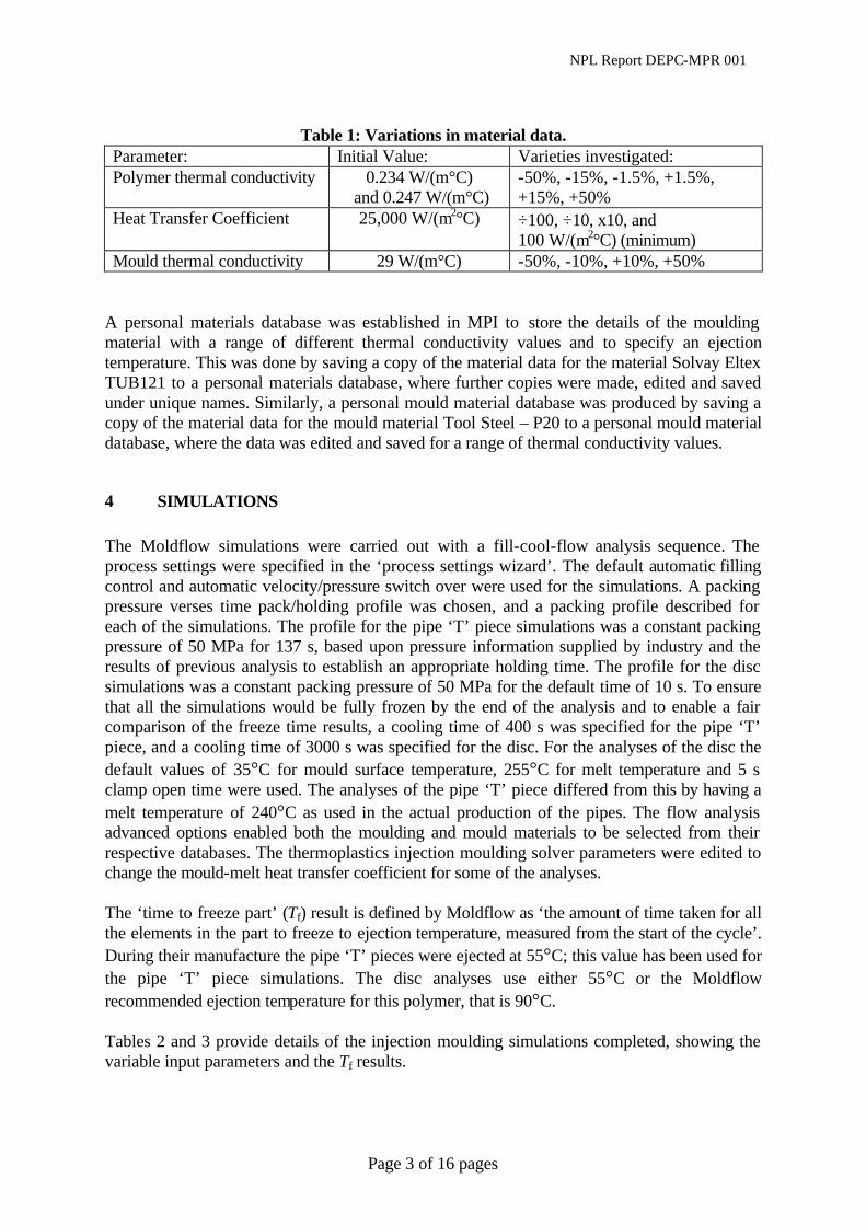
Table 1: Variations in material data.

Parameter: Initial Value: Varieties investigated: Polymer thermal conductivity 0.234 W/(m°C)

and 0.247 W/(m°C) -50%, -15%, -1.5%, +1.5%, +15%, +50%

Heat Transfer Coefficient 25,000 W/(m2°C) ÷100, ÷10, x10, and 100 W/(m2°C) (minimum)

Mould thermal conductivity 29 W/(m°C) -50%, -10%, +10%, +50% A personal materials database was established in MPI to store the details of the moulding material with a range of different thermal conductivity values and to specify an ejection temperature. This was done by saving a copy of the material data for the material Solvay Eltex TUB121 to a personal materials database, where further copies were made, edited and saved under unique names. Similarly, a personal mould material database was produced by saving a copy of the material data for the mould material Tool Steel – P20 to a personal mould material database, where the data was edited and saved for a range of thermal conductivity values.

4 SIMULATIONS The Moldflow simulations were carried out with a fill-cool-flow analysis sequence. The process settings were specified in the ‘process settings wizard’. The default automatic filling control and automatic velocity/pressure switch over were used for the simulations. A packing pressure verses time pack/holding profile was chosen, and a packing profile described for each of the simulations. The profile for the pipe ‘T’ piece simulations was a constant packing pressure of 50 MPa for 137 s, based upon pressure information supplied by industry and the results of previous analysis to establish an appropriate holding time. The profile for the disc simulations was a constant packing pressure of 50 MPa for the default time of 10 s. To ensure that all the simulations would be fully frozen by the end of the analysis and to enable a fair comparison of the freeze time results, a cooling time of 400 s was specified for the pipe ‘T’ piece, and a cooling time of 3000 s was specified for the disc. For the analyses of the disc the default values of 35°C for mould surface temperature, 255°C for melt temperature and 5 s clamp open time were used. The analyses of the pipe ‘T’ piece differed from this by having a melt temperature of 240°C as used in the actual production of the pipes. The flow analysis advanced options enabled both the moulding and mould materials to be selected from their respective databases. The thermoplastics injection moulding solver parameters were edited to change the mould-melt heat transfer coefficient for some of the analyses. The ‘time to freeze part’ (Tf) result is defined by Moldflow as ‘the amount of time taken for all the elements in the part to freeze to ejection temperature, measured from the start of the cycle’. During their manufacture the pipe ‘T’ pieces were ejected at 55°C; this value has been used for the pipe ‘T’ piece simulations. The disc analyses use either 55°C or the Moldflow recommended ejection temperature for this polymer, that is 90°C. Tables 2 and 3 provide details of the injection moulding simulations completed, showing the variable input parameters and the Tf results.


Page 4 of 16 pages

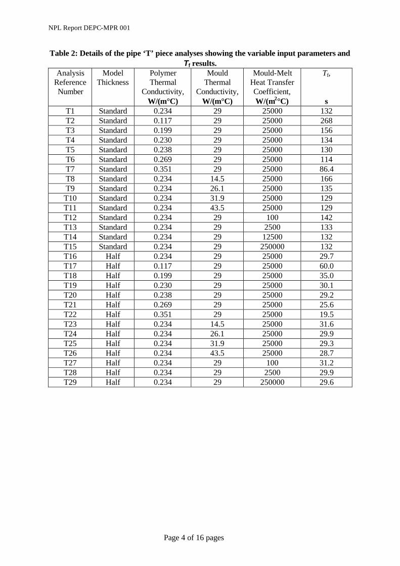
Table 2: Details of the pipe ‘T’ piece analyses showing the variable input parameters and Tf results.

Analysis Reference Number

Model Thickness

Polymer Thermal

Conductivity, W/(m°C)

Mould Thermal

Conductivity, W/(m°C)

Mould-Melt Heat Transfer Coefficient, W/(m2°C)

Tf, s

T1 Standard 0.234 29 25000 132 T2 Standard 0.117 29 25000 268 T3 Standard 0.199 29 25000 156 T4 Standard 0.230 29 25000 134 T5 Standard 0.238 29 25000 130 T6 Standard 0.269 29 25000 114 T7 Standard 0.351 29 25000 86.4 T8 Standard 0.234 14.5 25000 166 T9 Standard 0.234 26.1 25000 135 T10 Standard 0.234 31.9 25000 129 T11 Standard 0.234 43.5 25000 129 T12 Standard 0.234 29 100 142 T13 Standard 0.234 29 2500 133 T14 Standard 0.234 29 12500 132 T15 Standard 0.234 29 250000 132 T16 Half 0.234 29 25000 29.7 T17 Half 0.117 29 25000 60.0 T18 Half 0.199 29 25000 35.0 T19 Half 0.230 29 25000 30.1 T20 Half 0.238 29 25000 29.2 T21 Half 0.269 29 25000 25.6 T22 Half 0.351 29 25000 19.5 T23 Half 0.234 14.5 25000 31.6 T24 Half 0.234 26.1 25000 29.9 T25 Half 0.234 31.9 25000 29.3 T26 Half 0.234 43.5 25000 28.7 T27 Half 0.234 29 100 31.2 T28 Half 0.234 29 2500 29.9 T29 Half 0.234 29 250000 29.6


Page 5 of 16 pages

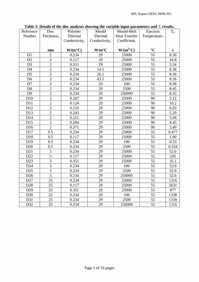
Table 3: Details of the disc analyses showing the variable input parameters and Tf results. Reference Number

Disc Thickness,

mm

Polymer Thermal

Conductivity,

W/(m°C)

Mould Thermal

Conductivity,

W/m°C

Mould-Melt Heat Transfer Coefficient,

W/(m2°C)

Ejection Temperature,

°C

Tf, s

D1 2 0.234 29 25000 55 8.36 D2 2 0.117 29 25000 55 16.8 D3 2 0.351 29 25000 55 5.54 D4 2 0.234 14.5 25000 55 8.36 D5 2 0.234 26.1 25000 55 8.36 D6 2 0.234 43.5 25000 55 8.36 D7 2 0.234 29 100 55 8.58 D8 2 0.234 29 2500 55 8.45 D9 2 0.234 29 250000 55 8.35 D10 2 0.247 29 25000 90 5.12 D11 2 0.124 29 25000 90 10.2 D12 2 0.210 29 25000 90 6.03 D13 2 0.243 29 25000 90 5.20 D14 2 0.251 29 25000 90 5.04 D15 2 0.284 29 25000 90 4.45 D16 2 0.371 29 25000 90 3.40 D17 0.5 0.234 29 25000 55 0.477 D18 0.5 0.117 29 25000 55 1.00 D19 0.5 0.234 29 100 55 0.53 D20 0.5 0.234 29 2500 55 0.524 D21 5 0.234 29 25000 55 52.6 D22 5 0.117 29 25000 55 105 D23 5 0.351 29 25000 55 35.1 D24 5 0.234 29 100 55 53.9 D25 5 0.234 29 2500 55 52.9 D26 5 0.234 29 250000 55 52.6 D27 25 0.234 29 25000 55 1316 D28 25 0.117 29 25000 55 2631 D29 25 0.351 29 25000 55 877 D30 25 0.234 29 100 55 1338 D31 25 0.234 29 2500 55 1318 D32 25 0.234 29 250000 55 1316


Page 6 of 16 pages

5 RESULTS 5.1 The Effect Of Variations In Polymer Thermal Conductivity On The Pipe ‘T’ Piece

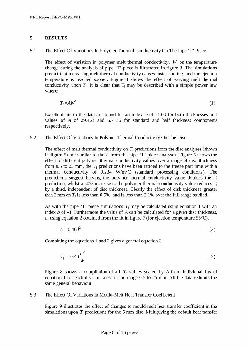
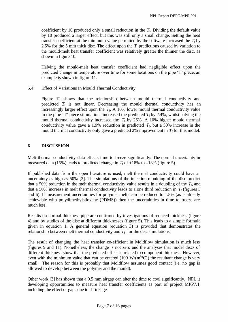
The effect of variation in polymer melt thermal conductivity, W, on the temperature change during the analysis of pipe ‘T’ piece is illustrated in figure 3. The simulations predict that increasing melt thermal conductivity causes faster cooling, and the ejection temperature is reached sooner. Figure 4 shows the effect of varying melt thermal conductivity upon Tf. It is clear that Tf may be described with a simple power law where:

Tf =AWb (1) Excellent fits to the data are found for an index b of -1.03 for both thicknesses and values of A of 29.463 and 6.7136 for standard and half thickness components respectively.

5.2 The Effect Of Variations In Polymer Thermal Conductivity On The Disc

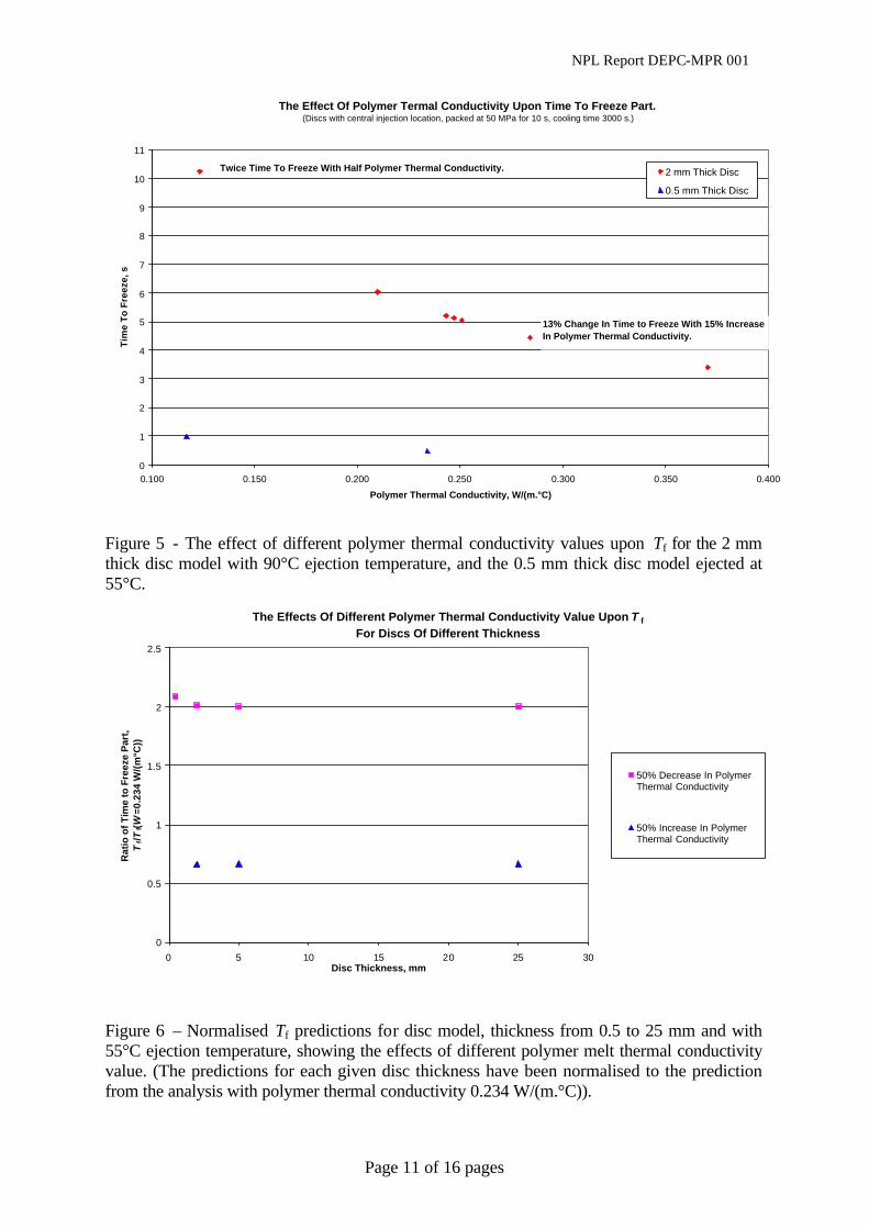
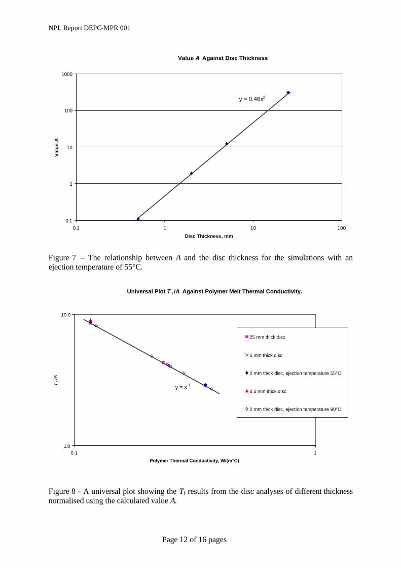
The effect of melt thermal conductivity on Tf predictions from the disc analyses (shown in figure 5) are similar to those from the pipe ‘T’ piece analyses. Figure 6 shows the effect of different polymer thermal conductivity values over a range of disc thickness from 0.5 to 25 mm, the Tf predictions have been ratioed to the freeze part time with a thermal conductivity of 0.234 W/m°C (standard processing conditions). The predictions suggest halving the polymer thermal conductivity value doubles the Tf prediction, whilst a 50% increase to the polymer thermal conductivity value reduces Tf by a third, independent of disc thickness. Clearly the effect of disk thickness greater than 2 mm on Tf is less than 0.5%, and is less than 2.1% over the full range studied. As with the pipe ‘T’ piece simulations Tf may be calculated using equation 1 with an index b of -1. Furthermore the value of A can be calculated for a given disc thickness, d, using equation 2 obtained from the fit in figure 7 (for ejection temperature 55°C). A = 0.46d2 (2) Combining the equations 1 and 2 gives a general equation 3.

WdT

2

f 46.0= (3)

Figure 8 shows a compilation of all Tf values scaled by A from individual fits of equation 1 for each disc thickness in the range 0.5 to 25 mm. All the data exhibits the same general behaviour.

5.3 The Effect Of Variations In Mould-Melt Heat Transfer Coefficient

Figure 9 illustrates the effect of changes to mould-melt heat transfer coefficient in the simulations upon Tf predictions for the 5 mm disc. Multiplying the default heat transfer


Page 7 of 16 pages

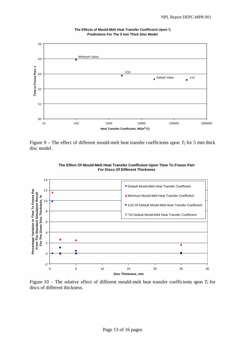
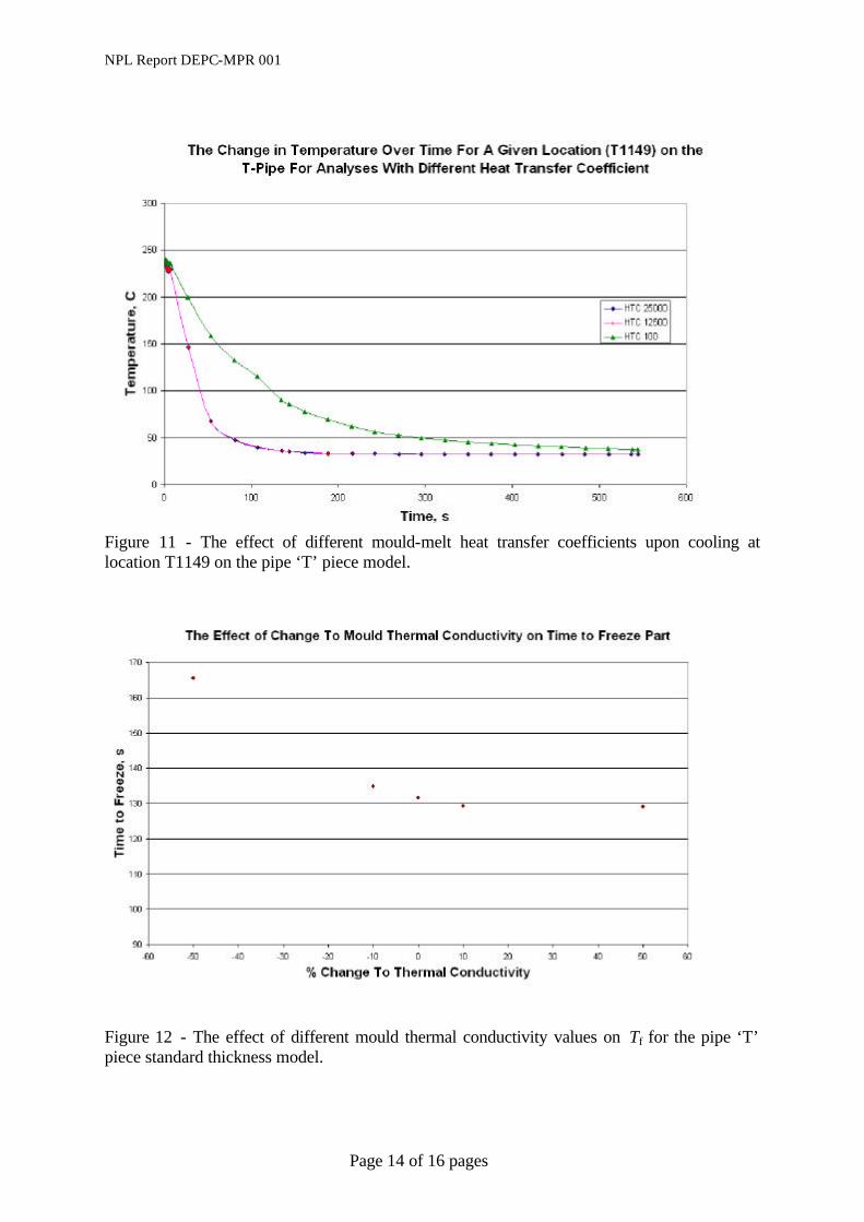
coefficient by 10 produced only a small reduction in the Tf. Dividing the default value by 10 produced a larger effect, but this was still only a small change. Setting the heat transfer coefficient at the minimum value permitted by the software increased the Tf by 2.5% for the 5 mm thick disc. The effect upon the Tf predictions caused by variation to the mould-melt heat transfer coefficient was relatively greater the thinner the disc, as shown in figure 10. Halving the mould-melt heat transfer coefficient had negligible effect upon the predicted change in temperature over time for some locations on the pipe ‘T’ piece, an example is shown in figure 11.

5.4 Effect of Variations In Mould Thermal Conductivity

Figure 12 shows that the relationship between mould thermal conductivity and predicted Tf is not linear. Decreasing the mould thermal conductivity has an increasingly larger effect upon the Tf. A 10% lower mould thermal conductivity value in the pipe ‘T’ piece simulations increased the predicted Tf by 2.4%, whilst halving the mould thermal conductivity increased the Tf by 26%. A 10% higher mould thermal conductivity value gave a 1.9% reduction in predicted Tf, but a 50% increase in the mould thermal conductivity only gave a predicted 2% improvement in Tf for this model.

6 DISCUSSION Melt thermal conductivity data effects time to freeze significantly. The normal uncertainty in measured data (15%) leads to predicted change in Tf of +18% to –13% (figure 5). If published data from the open literature is used, melt thermal conductivity could have an uncertainty as high as 50% [2]. The simulations of the injection moulding of the disc predict that a 50% reduction in the melt thermal conductivity value results in a doubling of the Tf, and that a 50% increase in melt thermal conductivity leads to a one third reduction in Tf (figures 5 and 6). If measurement uncertainties for polymer melts can be reduced to 1.5% (as is already achievable with polydimethylsiloxane (PDMS)) then the uncertainties in time to freeze are much less. Results on normal thickness pipe are confirmed by investigations of reduced thickness (figure 4) and by studies of the disc at different thicknesses (figure 5). This leads to a simple formula given in equation 1. A general equation (equation 3) is provided that demonstrates the relationship between melt thermal conductivity and Tf for the disc simulations. The result of changing the heat transfer co-efficient in Moldflow simulation is much less (figures 9 and 11). Nonetheless, the change is not zero and the analyses that model discs of different thickness show that the predicted effect is related to component thickness. However, even with the minimum value that can be entered (100 W/(m2°C)) the resultant change is very small. The reason for this is probably that Moldflow assumes good contact (i.e. no gap is allowed to develop between the polymer and the mould). Other work [3] has shown that a 0.5 mm airgap can alter the time to cool significantly. NPL is developing opportunities to measure heat transfer coefficients as part of project MPP7.1, including the effect of gaps due to shrinkage


Page 8 of 16 pages

Finally, the effect of mould thermal conductivity was briefly investigated (figure 12). For the model studied, decreasing the mould thermal conductivity value had greater effect upon the predicted Tf than increasing the value. This suggests the moulding material selected was well suited to the component studied. Compared to the effect of changes to polymer melt thermal conductivity, the effect of changes to mould thermal conductivity on the simulation predictions are small. This is because the thermal resistance of the metal mould is normally large compared to that of the polymer (due to the large ratio of polymer to mould thermal conductivity, 0.234 W/m°C to 29 W/m°C, ratio 1:124).

7 CONCLUSIONS The thermal conductivity of the polymer melt is a dominant heat transfer parameter in the injection moulding process. It has an inverse correlation with time to freeze the part, and appears largely independent of model thickness. At the normal uncertainty in measured data, uncertainties in melt thermal conductivity lead to similar uncertainties in time to freeze, thus any improvements to uncertainties in thermal conductivity data will result directly in improvements in cycle time predictions and consequently to productivity. A large change to the heat transfer coefficient is required to alter Moldflow predictions, good contact being assumed. There are noticeable effects upon predictions only at very low values (e.g. 100W/(m2°C)). The effects upon predictions that have been observed show that the relative importance of the mould-melt heat transfer coefficient is a function of the product geometry, where the heat transfer coefficient becomes increasingly important for thinner products. Uncertainties in mould thermal conductivity appear to have less effect than uncertainties in polymer thermal conductivity. However, relatively small increases (e.g. 10%) in mould thermal conductivity do give an improvement to time to freeze.

8 ACKNOWLEDGMENTS The authors would like to thank Eric Henry (Moldflow Ltd.), Paul Larter (Moldflow Ltd.) and Moldflow Ltd. for provision of the Moldflow Plastics Insight software, Angela Dawson (NPL) for materials measurement, and Mick Bull, Glynwed Pipe Systems Ltd. for advice and encouragement. This work is part funded by Eureka via the Aimtech project and part funded by Department of Trade and Industry (National Measurement System) via the Measurements for Processing and Performance (MPP) and Materials Infrastructure and International programmes. This document is deliverable two of milestone eight of project MPP7.1 and deliverable one of work package one of the Aimtech project.

9 REFERENCES 1. ASTM Standard D5930 2. Chakravorty, S., A Review of Requirements For Improved Methods Of Measuring Thermal

Properties Of Polymers. CMMT(A)246, 1999 3. Minutes of Third IAG and meetings held at RAPRA Technology, 16th October 2003, Annex

3


Page 9 of 16 pages

10 FIGURES

Figure 1 - Pipe ‘T’ piece model, showing the injection location and two of the locations from which results were obtained.

Figure 2 - 80 mm diameter disc model with a central injection location.


Page 10 of 16 pages

Figure 3 - The effect of different polymer thermal conductivity values on cooling at location T1717 on the pipe ‘T’ piece model.

Figure 4 - The effect of different polymer thermal conductivity values on Tf for the pipe ‘T’ piece model.

The Effect of Polymer Thermal Conductivity on Tf Of The Pipe 'T' Piece Model

1

10

100

1000

0.1 1Thermal Conductivity, W/(m.°C)

T f, s

Standard Thickness Model Predictions

Half Thickness Model Predictions

Fit To Standard Thickness Model Predictions

Fit To Half Thickness Model Predictions

y=29.463x-1.03

y=6.7136x-1.03


Page 11 of 16 pages

Figure 5 - The effect of different polymer thermal conductivity values upon Tf for the 2 mm thick disc model with 90°C ejection temperature, and the 0.5 mm thick disc model ejected at 55°C.

Figure 6 – Normalised Tf predictions for disc model, thickness from 0.5 to 25 mm and with 55°C ejection temperature, showing the effects of different polymer melt thermal conductivity value. (The predictions for each given disc thickness have been normalised to the prediction from the analysis with polymer thermal conductivity 0.234 W/(m.°C)).

The Effect Of Polymer Termal Conductivity Upon Time To Freeze Part.(Discs with central injection location, packed at 50 MPa for 10 s, cooling time 3000 s.)

0

1

2

3

4

5

6

7

8

9

10

11

0.100 0.150 0.200 0.250 0.300 0.350 0.400

Polymer Thermal Conductivity, W/(m.°C)

Tim

e T

o F

reez

e, s

2 mm Thick Disc

0.5 mm Thick Disc

Twice Time To Freeze With Half Polymer Thermal Conductivity.

13% Change In Time to Freeze With 15% Increase In Polymer Thermal Conductivity.

The Effects Of Different Polymer Thermal Conductivity Value Upon T f

For Discs Of Different Thickness

0

0.5

1

1.5

2

2.5

0 5 10 15 20 25 30Disc Thickness, mm

Rat

io o

f Tim

e to

Fre

eze

Par

t,

Tf/T

f(W=0

.234

W/(

m°C

))

50% Decrease In PolymerThermal Conductivity

50% Increase In PolymerThermal Conductivity


Page 12 of 16 pages

Figure 7 – The relationship between A and the disc thickness for the simulations with an ejection temperature of 55°C.

Figure 8 - A universal plot showing the Tf results from the disc analyses of different thickness normalised using the calculated value A.

Value A Against Disc Thickness

0.1

1

10

100

1000

0.1 1 10 100

Disc Thickness, mm

Val

ue

A

y = 0.46x2

Universal Plot T f /A Against Polymer Melt Thermal Conductivity.

1.0

10.0

0.1 1

Polymer Thermal Conductivity, W/(m°C)

Tf /A

25 mm thick disc

5 mm thick disc

2 mm thick disc, ejection temperature 55°C

0.5 mm thick disc

2 mm thick disc, ejection temperature 90°C

y = x-1


Page 13 of 16 pages

Figure 9 - The effect of different mould-melt heat transfer coefficients upon Tf for 5 mm thick disc model.

Figure 10 - The relative effect of different mould-melt heat transfer coefficients upon Tf for discs of different thickness.

The Effect Of Mould-Melt Heat Transfer Coefficient Upon Time To Freeze PartFor Discs Of Different Thickness

-2

0

2

4

6

8

10

12

14

0 5 10 15 20 25 30

Disc Thickness, mm

Per

cen

tag

e V

aria

tio

n In

Tim

e T

o F

reez

e P

art

Fro

m T

he

Sta

nd

ard

Sim

ula

tio

n R

esu

ltF

or

Th

e G

iven

Dis

c T

hic

knes

s, %

Default Mould-Melt Heat Transfer Coefficient

Minimum Mould-Melt Heat Transfer Coefficient

1/10 Of Default Mould-Melt Heat Transfer Coefficient

*10 Default Mould-Melt Heat Transfer Coefficient

The Effects of Mould-Melt Heat Transfer Coefficient Upon Tf

Predictions For The 5 mm Thick Disc Model

50

51

52

53

54

55

10 100 1000 10000 100000 1000000

Heat Transfer Coefficient, W/(m2°C)

Tim

e to

Fre

eze

Par

t, s

1/10

x10Default Value

Minimum Value


Page 14 of 16 pages

Figure 11 - The effect of different mould-melt heat transfer coefficients upon cooling at location T1149 on the pipe ‘T’ piece model.

Figure 12 - The effect of different mould thermal conductivity values on Tf for the pipe ‘T’ piece standard thickness model.


Page 15 of 16 pages

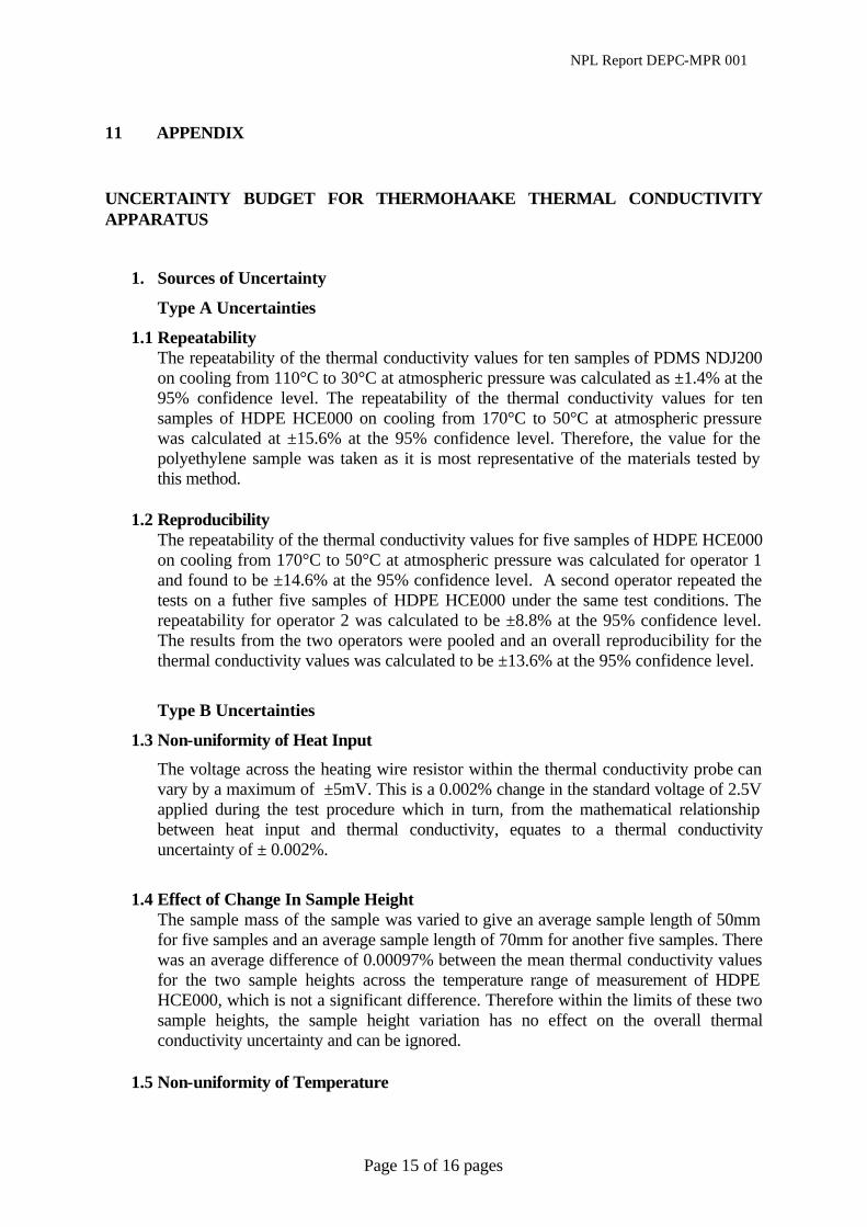
11 APPENDIX UNCERTAINTY BUDGET FOR THERMOHAAKE THERMAL CONDUCTIVITY APPARATUS

1. Sources of Uncertainty

Type A Uncertainties

1.1 Repeatability The repeatability of the thermal conductivity values for ten samples of PDMS NDJ200 on cooling from 110°C to 30°C at atmospheric pressure was calculated as ±1.4% at the 95% confidence level. The repeatability of the thermal conductivity values for ten samples of HDPE HCE000 on cooling from 170°C to 50°C at atmospheric pressure was calculated at ±15.6% at the 95% confidence level. Therefore, the value for the polyethylene sample was taken as it is most representative of the materials tested by this method.

1.2 Reproducibility The repeatability of the thermal conductivity values for five samples of HDPE HCE000 on cooling from 170°C to 50°C at atmospheric pressure was calculated for operator 1 and found to be ±14.6% at the 95% confidence level. A second operator repeated the tests on a futher five samples of HDPE HCE000 under the same test conditions. The repeatability for operator 2 was calculated to be ±8.8% at the 95% confidence level. The results from the two operators were pooled and an overall reproducibility for the thermal conductivity values was calculated to be ±13.6% at the 95% confidence level.

Type B Uncertainties

1.3 Non-uniformity of Heat Input

The voltage across the heating wire resistor within the thermal conductivity probe can vary by a maximum of ±5mV. This is a 0.002% change in the standard voltage of 2.5V applied during the test procedure which in turn, from the mathematical relationship between heat input and thermal conductivity, equates to a thermal conductivity uncertainty of ± 0.002%.

1.4 Effect of Change In Sample Height

The sample mass of the sample was varied to give an average sample length of 50mm for five samples and an average sample length of 70mm for another five samples. There was an average difference of 0.00097% between the mean thermal conductivity values for the two sample heights across the temperature range of measurement of HDPE HCE000, which is not a significant difference. Therefore within the limits of these two sample heights, the sample height variation has no effect on the overall thermal conductivity uncertainty and can be ignored.

1.5 Non-uniformity of Temperature


Page 16 of 16 pages

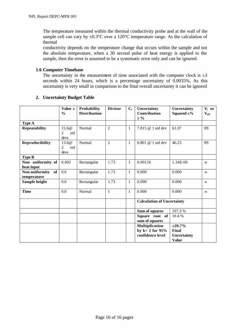
The temperature measured within the thermal conductivity probe and at the wall of the sample cell can vary by ±0.3°C over a 120°C temperature range. As the calculation of thermal conductivity depends on the temperature change that occurs within the sample and not the absolute temperature, when a 30 second pulse of heat energy is applied to the sample, then the error is assumed to be a systematic error only and can be ignored.

1.6 Computer Timebase The uncertainty in the measurement of time associated with the computer clock is ±3 seconds within 24 hours, which is a percentage uncertainty of 0.0035%. As this uncertainty is very small in comparison to the final overall uncertainty it can be ignored

2. Uncertainty Budget Table

Value ± %

Probability Distribution

Divisor Ci Uncertainty Contribution ± %

Uncertainty Squared ±%

Vi or Veff

Type A Repeatability 15.6@

2 std devs

Normal 2 1 7.815 @ 1 std dev 61.07 89

Reproducibility 13.6@ 2 std devs

Normal 2 1 6.801 @ 1 std dev 46.25 89

Type B Non- uniformity of heat input

0.002 Rectangular 1.73 1 0.00116 1.34E-06 ∞

Non-uniformity of temperature

0.0 Rectangular 1.73 1 0.000 0.000 ∞

Sample height 0.0 Rectangular 1.73 1 0.000

0.000 ∞

Time 0.0 Normal 1 1 0.000

0.000 ∞

Calculation of Uncertainty

Sum of squares 107.3 % Square root of

sum of squares 10.4 %

Multiplication by k= 2 for 95% confidence level

±20.7% Final Uncertainty Value

Documents

The Effect of Uncertainty in Heat Transfer Data on The ...resource.npl.co.uk/materials/polyproc/iag/april2005/effect_of... · The Effect of Uncertainty in Heat Transfer Data on The