Embed Size (px)
Citation preview
European Research Studies Journal
Volume XX, Issue 4B, 2017
pp. 727-753
The Effect of the Financial Crisis on Emerging Markets: A
Comparative Analysis of the Stock Market Situation Before
and After
Simon Grima1, Luca Caruana2 Abstract:
In this paper the authors present the findings of an analyses carried out to establish whether
the BRIC’s stock market returns were affected by the U.S. financial stress during the 2008
Financial Crisis. To do this the authors studied the relationship between the U.S. Stock Markets
and the BRIC countries’ stock and bond market returns.
They carried out a regression analysis which consisted of running an equation of the
dependent variable - the BRIC’s stock market returns, against a number of regressors -
explanatory variables, which include the U.S.’ industrial production, the U.S.’ unemployment
rate, the U.S.’S&P500, the Michigan confidence index, the BRIC’s consumer price index, the
industrial production, the Gross Domestic Product and the consumer price index of each
individual country; Brazil, Russia, India and China respectively.
Then the authors used a single-equation time series model to explain spillover effects
emanating from the US onto the BRIC markets. They analysed the whole data series from 2003
to 2014. Then sub-divided this data to analyse the post crisis effects on the BRICS equity
market. The index of Brazil, Russia, India and China respectively. - BOVESPA (Brazil),
MICEX (Russia), NIFTY (India) and China Security Index (CSI300) were the dependent
variables of the model.
Moreover, the model takes the US stock market index, the S&P500 as a benchmark variable.
Results obtained, revealed that the BRICs were subject to a spillover effect during and
following the financial crisis.
Keywords: BRICS, Financial Crisis, Emerging Markets
Original scientific paper UDK: 336.76:338.124.4
JEL classification: G01, G15
1 University of Malta, Department of Insurance, email: [email protected] 2 University of Malta, Department of Banking and Finance E-mail: [email protected]
The Effect of the Financial Crisis on Emerging Markets: A Comparative Analysis of the
Stock Market Situation Before and After
728
1. Introduction
The Goldman Sachs, 2003 paper “Dreaming with BRICs: The Path to 2050”,
highlighted that Emerging Markets (EM) are one of the drivers of global growth.
Noting that Brazil, Russia, India and China, collectively referred to as BRIC
countries, could in the light of the regulations, which are supportive of foreign
investment as well as the free flow of capital, further increase their potential
development (Bhar and Nikolova, 2008). In fact, BRIC countries represent a class of
the middle-income emerging market economy, distinctively large, which can prove
useful to enhance economic growth in the world economy (Marcelo et al., 2013).
Therefore, it is important to understand the way regional and global financial events
affect emerging market returns and the volatility of returns. Hence, to understand how
such markets respond when in financial stress (Bhar and Nikolova, 2008).
This paper focuses on the impact the financial crisis had on BRIC countries, with
respect to the United States, the original source of the crisis. The paper analyses the
contagion effects of financial shocks from the US to stock and bond markets in BRIC
countries and its effect on the volatility of such markets. Moreover, this paper also
analyses whether the BRIC countries were affected by US financial stress.
Many investors assume that the inclusion of emerging markets in investment portfolio
would enhance their risk-return tradeoff. Research shows that this is in fact true and
adding developing economies that are less correlated with advanced economies allows
for ideal diversification (Hallinan, 2011). However, in light of the past financial crisis,
this is highly debatable. Hence, this paper will also seek to answer questions imposed
by the modern portfolio theory, based on the work of Markowitz (1952) and the
Capital Asset Pricing Model (CAPM). That is, whether investors can improve their
positions by diversifying the portfolio and investing into different classes of financial
securities and whether developing countries really serve as diversification
opportunities to investors following the financial crisis (Aloui et al., 2011).
Since emerging equity markets are undergoing periods of constant change and
transformation, understanding the effect of integration with advanced economies such
as the U.S., Europe and Japan and assessing the weaknesses of the equity markets in
times of financial stress and during regional financial crisis, would prove beneficial to
investors, who are constantly seeking new ways of lowering their risks by
diversification (Chittedi, 2009).
2. Literature Review
Between 2006 and 2010, Gross Domestic Product (GDP) growth of the BRICs
outperformed growth in advanced economies. During this period, emerging-economic
market growth accounted for approximately 60% of worldwide GDP growth. Apart
from the fast-economic growth, emerging markets showed financial stability and
S. Grima, L. Caruana
729
economic resilience during the financial crisis of 2008. However, while GDP output
of advanced economies plunged, developing countries output remained constant
(World Economic Forum, 2012).
2.1 Contagion
Claessens et al. (2000), define contagion as the intensification of cross- market
integration after a shock in a country or group of countries. They explain that contagion
is defined by the degree to which stock prices move together across markets relevant
to movement when financial markets are not faced by financial stress. The variables
that make a country vulnerable to contagion and through which contagion is spread
are still unknown. Hence, it is difficult to propose other policies apart from more rigid
financial architecture to effectively reduce and prevent the risks of contagion.
Forbes and Rigobon (1999) examine stock market co-movements. They analysis the
different theoretical models as to how linkages between countries can be calculated.
Such statistical measures include correlation in asset returns, the probability of a
speculative attack and the transmission of shocks or volatility. They also explain what
contagion is and develop models on how to interpret spread mechanisms and suggest
that the standard tests to examine cross-market correlation in stock market returns is
biased and propose a simple method on how to adjust the correlation coefficient from
bias. They propose an understanding of why stock markets are integrated during
periods of financial stability. To study the spread of the U.S. financial crisis to BRIC
countries, Bianconi et al. (2013), use simple unconditional volatility measures, vector
autoregressions (VAR), cointegration, and conditional volatility and correlations
amongst stock and bond market returns. Thalassinos and Politis (2012) used Vector
Autoregressive Modelling for the USD and the oil prices.
Studies conducted by Eichengreen and Park (2008), refer to the recent financial crisis
to show that emerging markets where unable to disassociate themselves from the U.S.
financial crisis. Although developing markets and their exposure to U.S. financial
markets is limited, with enforced regulation on the market, they show that, one cannot
imply that the region is without any weakness. They also comment on the impression
that China’s economy grew so much that it segregates the whole region from U.S.
market spillovers. However, they note that although this may contain some truth, one
cannot deny that Asia’s economy is still linked to the United States both by trade and by
stock market co-movements. Dooley and Hutchison (2009), study the spillover effects
of the U.S. financial crisis to developing countries. The authors’ interest in the topic
is related to the fact that emerging markets took upon themselves reforms such as
increases in reserves and reduction of government deficits that should have isolated
them from financial shocks from other countries. Their paper analysis how emerging
markets’ CDS spreads were affected by U.S. financial shocks. They study about, what
news affected CDS spreads and the magnitude of these news on emerging markets.
Their research shows that the U.S. has large economic and statistical influence on
The Effect of the Financial Crisis on Emerging Markets: A Comparative Analysis of the
Stock Market Situation Before and After
730
emerging markets and that news moved markets consistently. However, the authors are
not sure whether the linkages between the U.S. and developing countries have changed
or whether the importance of events originating from the United States have changed.
This is often referred to as the ‘decoupling- recoupling’ debate. They report that
financial indicators show that emerging markets were decoupled from the United
States. It seemed that the growth rates of emerging and advanced economies were
heading in opposite directions. However, after the bankruptcy of Lehman Brothers in
September 2008, correlations between emerging markets and the U.S. also rose
substantially (markets recoupled). The paper also identified that major news, such as
the bankruptcy of Lehman Brothers and news on the real U.S. economy affected CDS
spreads in emerging markets.
Llaudes et al. (2010), analyze the characteristics of the initial crisis and the
heterogeneous transmission amongst emerging markets. The paper studies the impact
of the financial crisis on the decline in actual growth and decline in stock markets, as
well as the decline in credit growth. Since emerging markets where affected by an
external crisis, the paper focuses on exterior vulnerabilities of emerging markets. The
paper shows that countries that had linkages with advanced economies and are more
open to trade where severely hit by the crisis, they experienced steeper falls in output
during the crisis. While, countries that strengthened external weaknesses prior to the
financial crisis, later went into recession. They found a significant and a healthy
relationship between emerging markets’ reserves and their decline in growth during the
financial crisis.
Nikkinen et al. (2013) investigated the transmission of the US subprime crisis onto
BRIC countries and examined the impact of the financial crisis on the stock markets
and equity markets of the industrial and financial sectors. They use a bivariate GARCH-
BEKK model utilizing daily total return indices and estimate four pair-wise models.
They identify the extent of contagion by examining the industrial and financial sectors
of BRIC equity markets. Results show that there is evidence of contagion between the
US and BRIC markets due to direct linkages both in terms of returns and volatility and
that Russia and India’s equity returns as well as financial and industrial sector returns
where influenced by US equity market movements prior to the financial crisis. They
also found clear evidence of contagion, however, the authors show that only Russia’s
financial sector was severely affected by the fall of the Lehman Brothers.
Zouhair et al. (2014) examine the joint behavior of US and BRIC equity markets. The
authors found strong linkages between both stock markets during the US subprime
mortgage crisis. Result show evidence of contagion in Brazil and interdependence
between China, India and Russia. The study also shows high correlation coefficients for
Brazil, meaning that the economy is integrated with the United States in all periods
that were studied. Also, the study addresses the general idea that countries with low
integration in the global economy prove to be good diversification possibilities. This is
the case for India and China which have a low correlation coefficient compared to that
S. Grima, L. Caruana
731
of Brazil, these results are in line with studies by Aloui et al. (2011) and Bianconi et al.
(2013).
2.2 Cross-Market Linkages and integration
Aloui et al. (2011), examine the cross-market linkages and interdependences between
BRIC equity markets and the United States during the financial crisis. The authors
find that the dependency on the U.S. is more persistent in countries, which depend on
commodity prices such as Brazil and Russia – than for countries which economic
growth is dependent on finished products such as China and India. Chittedi (2009)
studied the long run co- integration relationship between BRIC countries and the U.S.,
UK and Japan using the Granger causality, Johansen co-integration and Error
Correction Mechanism. The authors found that the U.S. and Japan are influencing the
Indian stock market due to international trade activities. However, the study states that
India is far less influencing the UK, Brazil, China and Russia. They also show that the
BRICs and advanced economies where highly co-integrating during the period of the
study. Bianconi et al.’s (2013) results show that in fact for bond markets, India is
isolated from the other BRIC countries.
Morales and Gassie (2011) study the relationship between BRIC markets and energy
markets. The authors highlight the weak integration levels between the Chinese
financial markets, energy markets and the U.S. equity markets. They also show that
Brazil, Russia and India are more sensitive to financial shocks arising from the United
States as well as energy market instability. Bhar and Nikolova (2008) study the
linkages between the BRICs, their regions and the world by using a bivariate
EGARCH structure, this allows for time varying condition correlation of index equity
returns from such markets. They explain that the proposed model allows researchers
to analyze the impact of a number of events on BRIC markets and the correlation
equity index returns. The authors found evidence that India is the most integrated
country from the BRICs on both regional and global levels, followed by Brazil and
Russia. China is the most isolated country and hence the least volatile. This means
that China could be a great opportunity for investors to diversify their portfolio due to
the close nature of China’s financial markets. Results obtained indicate that none of
the BRIC countries impact the volatility of world market returns.
2.3 News, Volatility and their effect on correlations
Aggarwal et al. (1999) studied the events that have the largest impact on emerging stock
markets volatility. Results show that the periods of greater volatility shifts are inter-related
with important country-specific political, social and economic events such as the Mexican
Crisis and the Marcos-Aquino conflict in Philippines.
Bae and Karolyi (1994) results suggest that news from a particular market seem to affect
the short-term volatility of stock prices in foreign markets. They studied the relationship

The Effect of the Financial Crisis on Emerging Markets: A Comparative Analysis of the
Stock Market Situation Before and After
732
of the joint dynamics of the Nikkei stock average and the S&P 500 stock index over the
1988-1992 period. The authors noted that bad news from both local and foreign markets
seem to have a bigger impact on return volatility than good news.
Beirne et al. (2009), studied the volatility spillover from advanced economies to emerging
economies. They found that that volatility in emerging stock markets tended to be higher
in periods where mature markets where in turbulence periods.
Bianconi et al. (2013), explain that the behavior of asset classes affects the co-integration
relationship between U.S. financial stress and BRIC nations. Using Multivariate GARCH
models and dynamic conditional correlations, they shed light on the role of news and
volatility and explore how these affect the correlations between national stock markets
during the global financial crisis. Contrary to what was found by Mun and Brooks (2012),
who show that news does not have a significant effect on the correlations and that the
majority of correlations are strongly explained by volatility, Bianconi et al. (2013), note
that news and volatility are equally important for stock returns, but news are less
important than the volatility in BRIC markets when referring to bond and stock markets
returns altogether.
2.4 Stock and bond market Correlations and Yield Spreads
Baur (2007) shows that in developing countries stock-bond market correlations are
highly influenced by cross-country influences rather than stock and bond market
interaction. He tests the relationship of cross-country, cross- asset stock and bond
market linkages. Results show that U.S stock markets influences stock and bond
market returns of the eight developed countries. Aslanidis and Christiansen (2012)
adopt quantile regressions to study the realized stock-bond correlation based upon high
frequency returns. They explain that when the correlation is highly positive or highly
negative, correlation dependence behaves differently.
Bunda et al. (2009) examine the co-movement in emerging bond market linking to
internal and external factors during high market volatility episodes. They analysis
eighteen emerging markets between 1997 and 2008 and proposed a conceptual
framework based on emerging market spreads and cumulative correlations. The study
sheds light on the drop in emerging markets spreads and the factors that contributed
to this. They note that the decline was not only led by external factors but also to the
fact that emerging countries improved their country fundamentals. They show that the
period between 2003 and 2008 had very low levels of contagion in the bond markets.
This period was characterized by the global financial crisis and explain that
correlations between bond markets increased after the crisis. They also show that the
mentioned phenomenon explains the increase in emerging bond markets’ volatility.
Siklos (2011), studies twenty-two emerging markets to understand the determinants
of bond yield spreads in the period 1998-2009. He examines the linkage between
S. Grima, L. Caruana
733
volatility and bond yield spreads. The study shows that emerging markets aren’t all
affected in the same way and cannot be treated equally. Results show that Asian bond
markets were decoupled from other developing economies during the financial crisis,
agreeing with Bianconi et al. (2013) with regards to the isolation of Indian bond
markets.
Bianconi et al. (2013), show that BRICs cannot be isolated from the financial stress
posed by the United States. Results show that Brazil and Russia are very much likely
to suffer financial stress, however, India is the least correlated market. They also
investigate whether emerging markets can prove to be good diversification
opportunities for investors. The study shows that during that period, China’s stock
markets respond less to financial stress when compared to other nations. Also, Indian
bond markets seem to be isolated from external factors and hence are less influenced
by financial stress and external factors posed by the United States.
3. Methodology
3.1 Sample selection
The sample data for the whole period, 2003 to 2014, was collected using the Thompson
Reuters platform. This data was split into two periods. The first period related to the whole
period from 2003 to 2014, the second data period related to the period after the financial
crisis between 2009 and 2014. Due to lack of monthly data for the gross domestic product,
the researcher chose to use industrial production (IP) as a proxy, since except in the case
of Brazil, it correlates well with the former variable. The authors used the Eviews
application software to conduct the correlation analysis between the two variables for all
countries. Although the authors did not find serious correlation between Brazil’s GDP and
industrial production, they still felt that this variable was the best proxy to use for GDP
data.
3.2 Research Model
The researchers used a single-equation time series model to try and explain spillover
effects emanating from the US onto the leading emerging markets. This model was
chosen so as to enable them to focus on the first two moments, that is, the mean and
the constant variance. The research assumes a normal distribution and does not
analyze the skewness and kurtosis of the data. This requires the authors to consider a
time-variant variance, which is not possible with other models such as the EGARCH.
This would also mean that the third and fourth moments do not affect the analysis of
the study.
The researchers first analyze the whole data series, that is from 2003 to 2014. Then
analyze the post crisis effects on the emerging equity market. The dependent variable
of the model will be the index of Brazil, Russia, India and China respectively. Hence,
the authors use the following indices: BOVESPA (Brazil), MICEX (Russia), NIFTY
The Effect of the Financial Crisis on Emerging Markets: A Comparative Analysis of the
Stock Market Situation Before and After
734
(India) and China Security Index (CSI300).
The model will take the US stock market index- the S&P500 as a benchmark variable.
The independent variables included in the model are the US industrial production
acting as a substitute to the GDP, the US unemployment rate (UR), US non-farm
payrolls (NFP) and the Michigan Confidence Index (MCI) as well as the industrial
production of each of the BRIC countries and their consumer price index (CPI). By
considering these variables in this research model, the authors can understand whether
the BRICs’ equity markets were isolated from the US financial stress.
3.3 Method of Analysis
The authors first plotted the data to determine visually, whether the data collected is
stationary or not, and then conducted an augmented Dickey-Fuller unit-root test to test
for autocorrelation and whether the variables have a unit root. If the variables had an
ADF test statistic lower than the test critical value of 1%, this meant that the data has
a unit-root and the variable is non-stationary.
The researchers used the EViews software package to analyze the regression. Through
the various tests available on EViews the authors were able to test whether the model
is econometrically correct and test it using diagnostic checking. One important aspect
of EViews is that it allows the researcher to use regression analysis with the aim to
explain how the independent variables affect the dependent variable. The authors used
EViews to explain whether the BRIC equity indices where indeed affected by the US
financial stress.
In
2 3 4 5 6
= B
2 3
1
BOVESPA = B (S&P500) + B (IP ) + B (UR ) + B (NFP ) + B (MCI )
BR 1 2 US 3 US 4 US 5 US
+ B (IP ) + B (CPI ) + U
6 Br 7 Br
NIFTY = B (S&P500) + B (IP ) + B (UR ) + B (NFP ) + B (MCI ) + B
(IP ) + B (CPI ) + U In 7
MICEX = B
In
(S&P500) + B (IP ) + B (UR ) + B (NFP ) + B (MCI ) +
Ru 1 2 US 3 US 4 US 5 US
B (IP ) + B (CPI ) + U
6 Ru 7 Ru
S H C O M P Ch 1 (S&P500) + B (IP ) + B (UR ) + B (NFP ) + B (MCI
+ B (IP ) + B (CPI ) + U
US US US US
US US 4 US 5
)
US
S. Grima, L. Caruana
735
They compare the two sub-periods against each other and made reference to the various
statistical indicators as shown by the regression. They then tested for the significance of
the variables and checked whether these should be included in the model. Variables
found to be statistically significant meant that they explained the dependent variable.
On the other hand, if the variable was not significant, the variable did not have an effect
on the stock market. The authors then interpreted the meaning of the coefficient term
as well as the p-values and ran a white-test to check for heteroscedasticity, then
computed the F-statistic to check whether the regression’s variables were jointly
statistically significant. Then they checked the R-squared, to see how much of the
dependent variable was explained by the model and what was captured by the error
term (u).
3.4 Limitations of the theoretical model
The authors note that this model has some limitations that result in endogeneity. The
first limitation of the model is ‘the omitted variable bias’, which generally results from
limited sources of data. Clarke (2005) explains that it is difficult to include all the
variables that influence the dependent variable in the regression equation, hence, the
omitted variable bias is inevitable. Also, a second limitation to the model, is
‘simultaneity’, also referred to as ‘the direction of causality’. The authors refer to the
fact that some independent variables are dependent on the dependent variable, hence,
the independent variables can have some correlation with the error term.
As noted above, the authors were also faced with limited data, due to the fact that the
GDP variable was only available quarterly or annually. Therefore, they used a proxy
for GDP. Moreover, for India’s NIFTY stock index the authors only managed to obtain
data from 2005, which resulted in fewer observations, limiting the ability to analyse
the effect of the financial crisis on India.
4. Tests and Conclusions
4.1 Testing for Stationarity
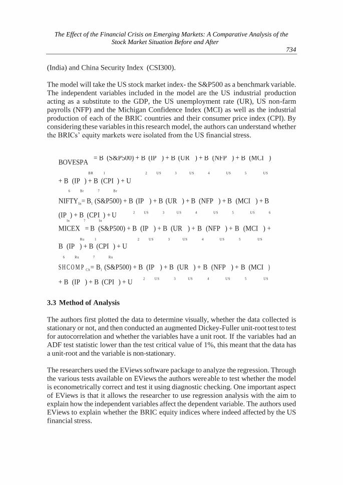
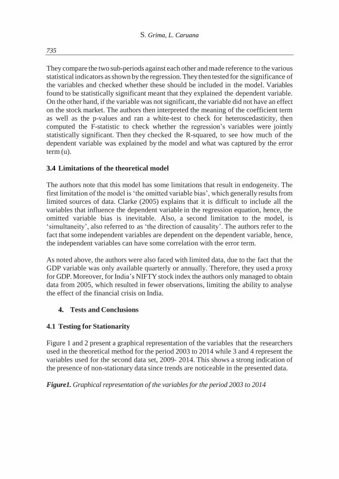
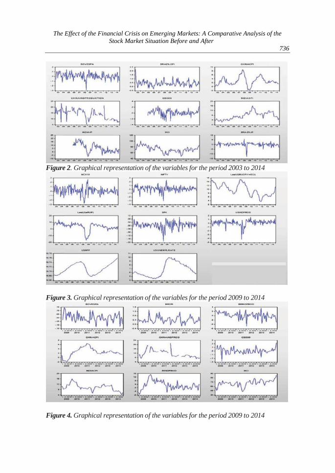
Figure 1 and 2 present a graphical representation of the variables that the researchers
used in the theoretical method for the period 2003 to 2014 while 3 and 4 represent the
variables used for the second data set, 2009- 2014. This shows a strong indication of
the presence of non-stationary data since trends are noticeable in the presented data.
Figure1. Graphical representation of the variables for the period 2003 to 2014
The Effect of the Financial Crisis on Emerging Markets: A Comparative Analysis of the
Stock Market Situation Before and After
736
Figure 2. Graphical representation of the variables for the period 2003 to 2014
Figure 3. Graphical representation of the variables for the period 2009 to 2014
Figure 4. Graphical representation of the variables for the period 2009 to 2014
S. Grima, L. Caruana
737
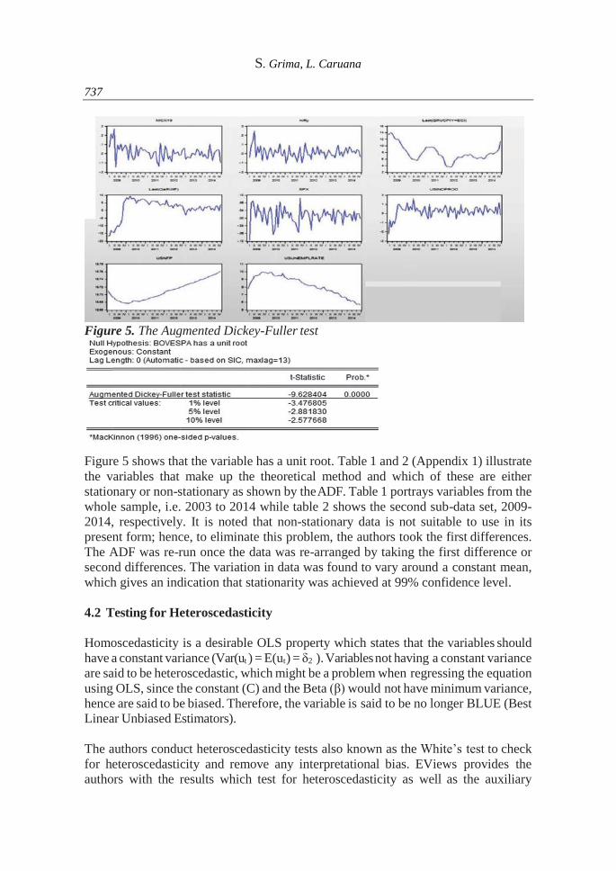
Figure 5. The Augmented Dickey-Fuller test
Figure 5 shows that the variable has a unit root. Table 1 and 2 (Appendix 1) illustrate
the variables that make up the theoretical method and which of these are either
stationary or non-stationary as shown by the ADF. Table 1 portrays variables from the
whole sample, i.e. 2003 to 2014 while table 2 shows the second sub-data set, 2009-
2014, respectively. It is noted that non-stationary data is not suitable to use in its
present form; hence, to eliminate this problem, the authors took the first differences.
The ADF was re-run once the data was re-arranged by taking the first difference or
second differences. The variation in data was found to vary around a constant mean,
which gives an indication that stationarity was achieved at 99% confidence level.
4.2 Testing for Heteroscedasticity
Homoscedasticity is a desirable OLS property which states that the variables should
have a constant variance (Var(ut ) = E(ut ) = δ2 ). Variables not having a constant variance
are said to be heteroscedastic, which might be a problem when regressing the equation
using OLS, since the constant (C) and the Beta (β) would not have minimum variance,
hence are said to be biased. Therefore, the variable is said to be no longer BLUE (Best
Linear Unbiased Estimators).
The authors conduct heteroscedasticity tests also known as the White’s test to check
for heteroscedasticity and remove any interpretational bias. EViews provides the
authors with the results which test for heteroscedasticity as well as the auxiliary
The Effect of the Financial Crisis on Emerging Markets: A Comparative Analysis of the
Stock Market Situation Before and After
738
regression, which is a useful source when determining the source of heteroscedasticity
of a multiple variable regression.
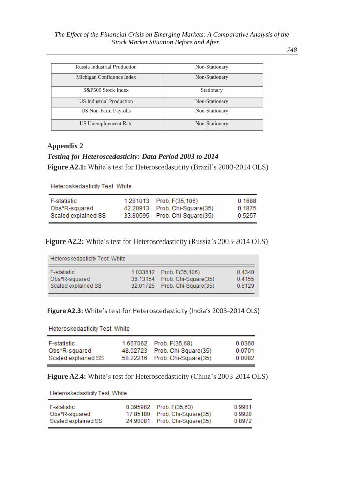
In the case of the White’s test, the null hypothesis states that there is homoscedasticity,
while the alternative hypothesis states that heteroscedasticity is present in the
regression. If the p-value are more than 5% or 0.05, it is assumed that there is no
presence of heteroscedasticity. On the other hand, if the p-values are lower than 0.05,
the data has to be corrected to support the assumption of homoscedasticity. The
software package used gives a quick option that adjusts data to account for
heteroscedasticity. The results of the White’s test for the variables used are shown in
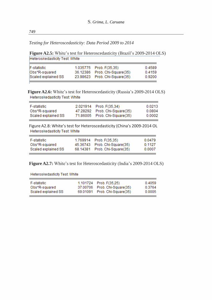
appendix 2 (figures A2.1 to A2.8) and most of the data have high p-values, hence the
null hypothesis was accepted, meaning that the data is homoscedastic. On the other
hand, for cases such as India, data were adjusted using heteroscedasticity-consistent
standard errors.
In Appendix 3 (Figures A3.1-A3.4), the authors illustrate how the OLS and standard
errors changed after adjusting for heteroscedasticity when compared to that illustrated
in Appendix 1.
4.3 Result Analysis
Once diagnostic checks were carried out, the authors were able to analyze results from
the OLS estimations (Appendix 3).
4.3.1 The OLS’s descriptive statistics
Brazil
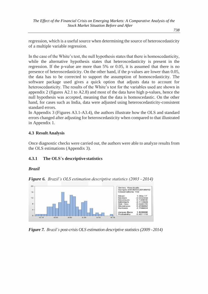
Figure 6. Brazil’s OLS estimation descriptive statistics (2003 - 2014)
Figure 7. Brazil’s post-crisis OLS estimation descriptive statistics (2009 - 2014)
S. Grima, L. Caruana
739
Brazil’s data for the whole period is symmetrical with a value of 0.26 and slightly
skewed to the right. The kurtosis of Brazil’s overall data is 2.8 and is very close to
kurtosis of normal distribution (±3.0), however when compared, the estimation’s data
is flatter than normal distribution with a wider peak, meaning that the data is widely
spread around the mean. Further to that, the Jarque-Bera test probability well exceed
the 0.01 p-value. Therefore, the data follows a normal distribution.
Brazil’s post-crisis regression, shows descriptive statistics similar to the overall
estimation period. The skewness is 0.17, which means that the data is lightly skewed
to the right close to symmetry. The kurtosis is 2.69 and when compared to the kurtosis
of normal distribution it is found that the data is flatter and widely spread around the
mean. The Jarque-Bera test statistic is very low 0.64, however, the p-value is 0.72
which exceeds the 0.01 value. Therefore, the data follows a normal distribution.
Russia
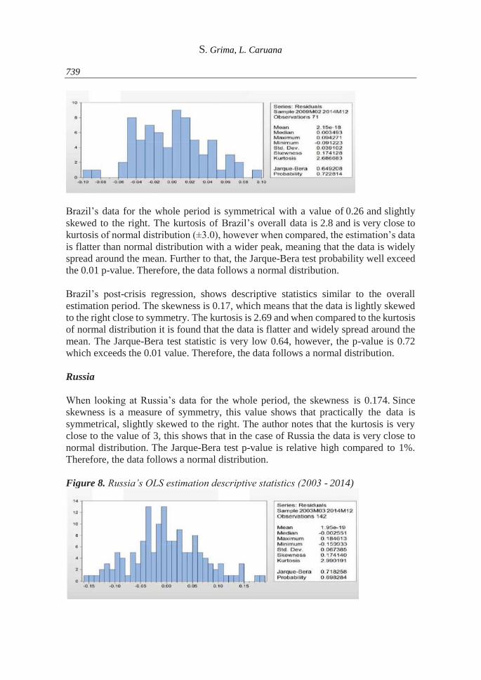
When looking at Russia’s data for the whole period, the skewness is 0.174. Since
skewness is a measure of symmetry, this value shows that practically the data is
symmetrical, slightly skewed to the right. The author notes that the kurtosis is very
close to the value of 3, this shows that in the case of Russia the data is very close to
normal distribution. The Jarque-Bera test p-value is relative high compared to 1%.
Therefore, the data follows a normal distribution.
Figure 8. Russia’s OLS estimation descriptive statistics (2003 - 2014)
The Effect of the Financial Crisis on Emerging Markets: A Comparative Analysis of the
Stock Market Situation Before and After
740
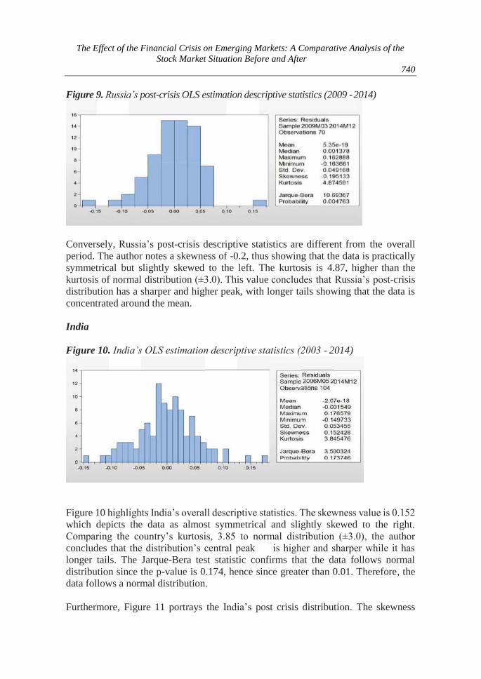
Figure 9. Russia’s post-crisis OLS estimation descriptive statistics (2009 - 2014)
Conversely, Russia’s post-crisis descriptive statistics are different from the overall
period. The author notes a skewness of -0.2, thus showing that the data is practically
symmetrical but slightly skewed to the left. The kurtosis is 4.87, higher than the
kurtosis of normal distribution (±3.0). This value concludes that Russia’s post-crisis
distribution has a sharper and higher peak, with longer tails showing that the data is
concentrated around the mean.
India
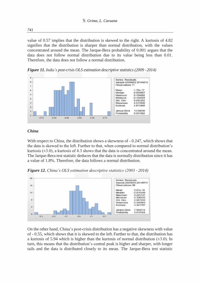
Figure 10. India’s OLS estimation descriptive statistics (2003 - 2014)
Figure 10 highlights India’s overall descriptive statistics. The skewness value is 0.152
which depicts the data as almost symmetrical and slightly skewed to the right.
Comparing the country’s kurtosis, 3.85 to normal distribution (±3.0), the author
concludes that the distribution’s central peak is higher and sharper while it has
longer tails. The Jarque-Bera test statistic confirms that the data follows normal
distribution since the p-value is 0.174, hence since greater than 0.01. Therefore, the
data follows a normal distribution.
Furthermore, Figure 11 portrays the India’s post crisis distribution. The skewness
S. Grima, L. Caruana
741
value of 0.57 implies that the distribution is skewed to the right. A kurtosis of 4.82
signifies that the distribution is sharper than normal distribution, with the values
concentrated around the mean. The Jarque-Bera probability of 0.001 argues that the
data does not follow normal distribution due to its value being less than 0.01.
Therefore, the data does not follow a normal distribution.
Figure 11. India’s post-crisis OLS estimation descriptive statistics (2009 - 2014)
China
With respect to China, the distribution shows a skewness of - 0.247, which shows that
the data is skewed to the left. Further to that, when compared to normal distribution’s
kurtosis (±3.0), a kurtosis of 4.3 shows that the data is concentrated around the mean.
The Jarque-Bera test statistic deduces that the data is normally distribution since it has
a value of 1.8%. Therefore, the data follows a normal distribution.
Figure 12. China’s OLS estimation descriptive statistics (2003 - 2014)
On the other hand, China’s post-crisis distribution has a negative skewness with value
of - 0.55, which shows that it is skewed to the left. Further to that, the distribution has
a kurtosis of 5.94 which is higher than the kurtosis of normal distribution (±3.0). In
turn, this means that the distribution’s central peak is higher and sharper, with longer
tails and the data is distributed closely to its mean. The Jarque-Bera test statistic
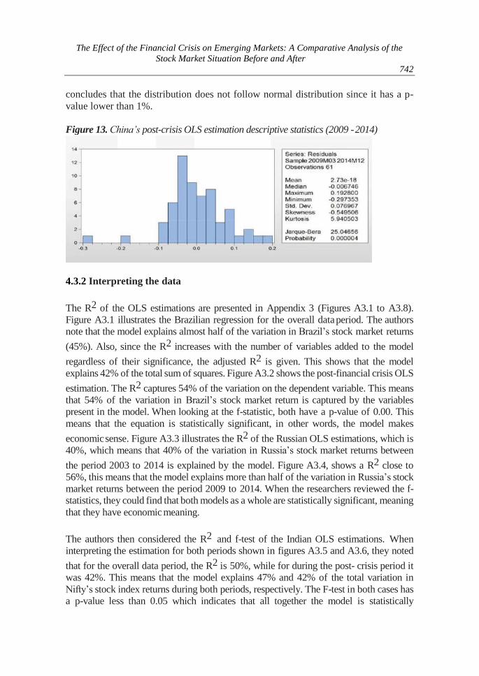
The Effect of the Financial Crisis on Emerging Markets: A Comparative Analysis of the
Stock Market Situation Before and After
742
concludes that the distribution does not follow normal distribution since it has a p-
value lower than 1%.
Figure 13. China’s post-crisis OLS estimation descriptive statistics (2009 - 2014)
4.3.2 Interpreting the data
The R2 of the OLS estimations are presented in Appendix 3 (Figures A3.1 to A3.8).
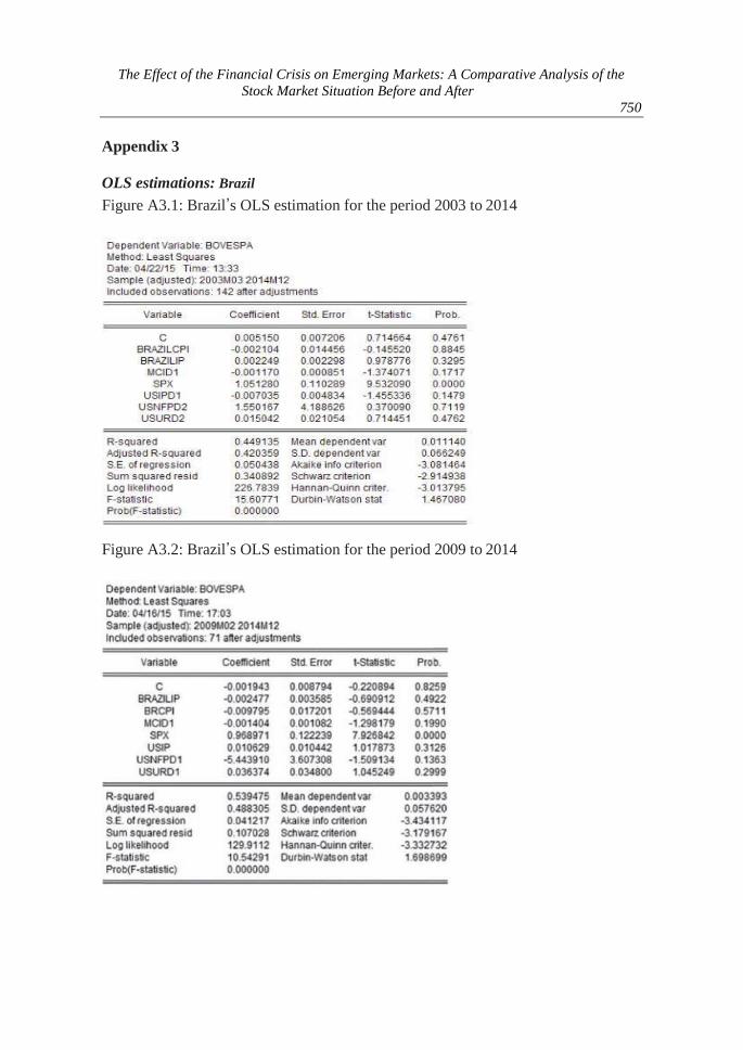
Figure A3.1 illustrates the Brazilian regression for the overall data period. The authors
note that the model explains almost half of the variation in Brazil’s stock market returns
(45%). Also, since the R2 increases with the number of variables added to the model
regardless of their significance, the adjusted R2 is given. This shows that the model
explains 42% of the total sum of squares. Figure A3.2 shows the post-financial crisis OLS
estimation. The R2 captures 54% of the variation on the dependent variable. This means
that 54% of the variation in Brazil’s stock market return is captured by the variables
present in the model. When looking at the f-statistic, both have a p-value of 0.00. This
means that the equation is statistically significant, in other words, the model makes
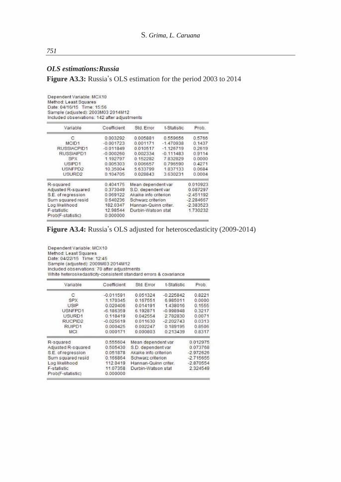
economic sense. Figure A3.3 illustrates the R2 of the Russian OLS estimations, which is
40%, which means that 40% of the variation in Russia’s stock market returns between
the period 2003 to 2014 is explained by the model. Figure A3.4, shows a R2 close to
56%, this means that the model explains more than half of the variation in Russia’s stock
market returns between the period 2009 to 2014. When the researchers reviewed the f-
statistics, they could find that both models as a whole are statistically significant, meaning
that they have economic meaning.
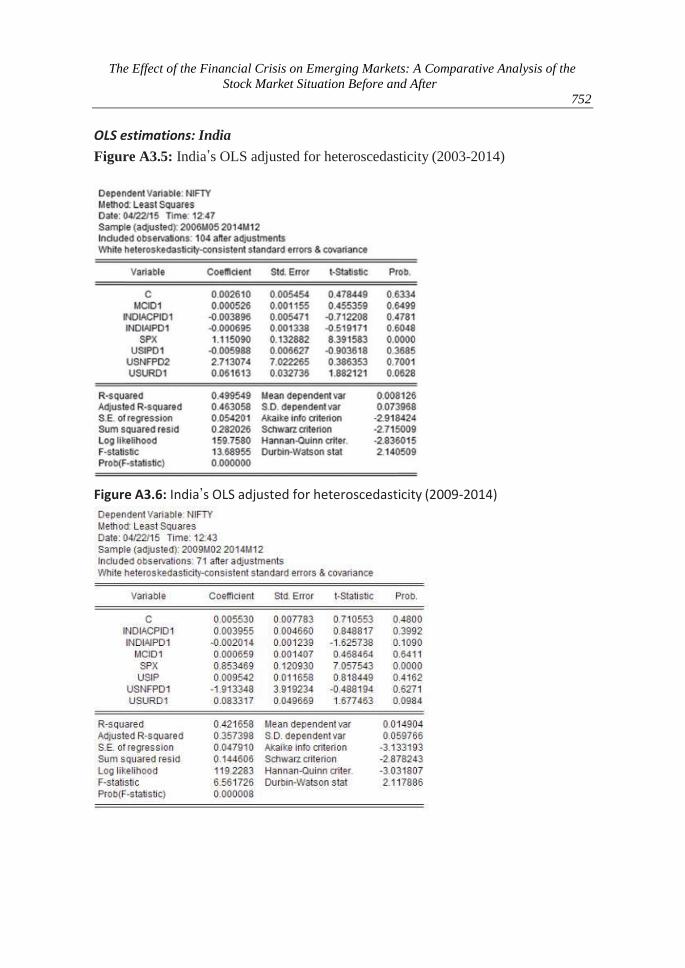
The authors then considered the R2 and f-test of the Indian OLS estimations. When
interpreting the estimation for both periods shown in figures A3.5 and A3.6, they noted
that for the overall data period, the R2 is 50%, while for during the post- crisis period it
was 42%. This means that the model explains 47% and 42% of the total variation in
Nifty’s stock index returns during both periods, respectively. The F-test in both cases has
a p-value less than 0.05 which indicates that all together the model is statistically

S. Grima, L. Caruana
743
significant.
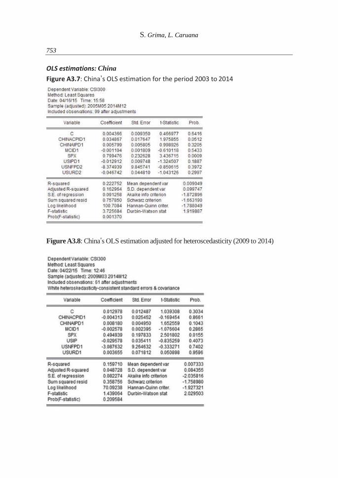
Finally, the authors considered the R2 and f-test of the China’s OLS estimations. As noted
in figures A3.7 and A3.8, the model only explains 22% for the overall period, and 16%
of the total variation in China’s stock market returns for the post-crisis period. This means
that the researchers left out other important factors that affect China stock market index
returns, specifically not including all variables in the model. As with regards the F-test,
for the overall data period the model is statistically significant as a whole with a p-value
lower than 0.05. Conversely, for the post-crisis analysis, the f-statistic has a p-value of 0.21,
thus the model as a whole is not statistically significant.
The authors also looked at the statistical significance of the beta coefficients and compared
it to previous research. A variable is said to be statistically significant when the p-value is
lower than 0.05. Eichengreen and Park (2008) argue that China’ s economy grew so much
that the whole region was isolated from the US financial stress. Morales and Gassie (2011)
who study the relationship between BRIC financial markets, energy markets and US
markets, state that there are weak integration levels between the three markets. The
researchers note that the results obtained are not in line with the research carried out by
the aforementioned. Table 4.3.4.2 shows China’s OLS estimation. This shows that the US
S&P500 stock index is individually statistically significant. As a result, this indicates that
China’s stock market returns are in reality not protected against US financial stress. Also,
the researchers found that the relationship between China’s stock market returns (CSI300)
and US Stock Market returns (S&P500) is in line with findings by previous authors.
Showing that the US had a more severe impact during the whole period, which
diminished after the financial crisis. Moreover, the paper by Morales and Gassie (2011)
concludes that Brazil, Russia and India are more susceptible to US financial shocks. This
is in line with the results acquired by the researchers where the SPX variable (S&P500)
is statistically significant in all periods, having a p-value of 0.000. Also, the beta
coefficients for these countries are quite high in both periods analyzed and confirm other
author’s findings.
The researchers refer to the paper by Bianconi et al. (2013) since their results are close to
the ones shown in this paper. The study conducted by Bianconi et al. (2013) shows that
the BRICs cannot be considered as segregated from the financial stress emanating from
the United States. Bianconi et al. (2013) state that Brazil and Russia are very likely to
suffer from spillovers transmitted from the US, however, it is shown that India is the least
correlated market. In addition to that, the authors outline that Russia’s Micex stock market
returns where affected not only by the US S&P500 stock index but also by the US’s
unemployment rate. They explain that the US unemployment rate’s beta coefficient is in
line with the findings of previous authors, hence an increase in US unemployment rate
leads to an increase in Russia’s stock market returns. In turn, both periods were affected
by the unemployment rate on similar levels. The results illustrated in Tables 1 and 2 below
show that the results obtained are in-line with Bianconi et al.’s (2013) interpretation.
However, the researchers’ findings about India differ. The results show that India is

The Effect of the Financial Crisis on Emerging Markets: A Comparative Analysis of the
Stock Market Situation Before and After
744
integrated and affected by the US financial stress as equivalent to Brazil and Russia.
In conclusion, from the results obtained the authors deduce that the US S&P500 stock
market index influences the BRICs stock market returns, mainly the BOVESPA, MICEX
Index, Russia (MCX10), NIFTY and CSI300 stock returns in both periods. In other
words, the BRIC emerging market economies are still not isolated from the major
spillover effect transmitted from the US. In reality, irrespective of the volatility in both
periods, the US still has a big impact on the stock returns on emerging economies.
Table 1. Table illustrating the variable’s Coefficient and p-values for Brazil and
Russia
Table 2. Table illustrating the variable’s Coefficient and p-values for India and
China
References:

S. Grima, L. Caruana
745
Aggarwal, R., Inclan, C. and Leal, R. 1999. Volatility in Emerging Stock Markets. Journal of
Financial Quantitative Analysis.
Gusti Ngurah Agung, I. 2009. Time Series Data Analysis Using Eviews. Chichester, West
Sussex, Wiley publishers.
Aloui, R., Nguyen, D.K. and Ben Aïssa, M.S. 2011. Global financial crisis, extreme
interdependences, and contagion effects: The role of economic structure? Elsevier.
Angkinand, A.P., Barth, J.R. and Hyeongwoo, K. 2009. Spillover effects from the U.S.
financial crisis: Some time-series evidence from national stock returns. Paper.
Edward Elgar Publishing.
Aslanidis, N. and Christiansen, C. 2012. Quantiles of the Realized Stock- Bond Correlation and
Links to the Macroeconomy. Research Paper.
Bae, K.H. and Karolyi, A. 1994. Good news, bad news and international spillovers of stock
return volatility between Japan and the U.S. Finance Journal. Elsevier.
Balasubramaniam, K. 2015 ‘What Impact Does a Higher Non-Farm Payroll Have On The
Forex Market?’.
Baur, D.G. 2007. Stock-bond co-movements and cross-country linkages. IIIS Discussion
Paper. Institute for International Integration Studies.
Beirne, J., Caporale, G. M., Schulze-Ghattas, M. and Spagnolo, N. 2009. Volatility
spillovers and contagion from mature to emerging stock markets. Working Paper.
Economics and Finance.
Bhar, R. and Nikolova, B. 2008. Return, volatility spillovers and dynamic correlation in the
BRIC equity markets: An analysis using a bivariate EGARCH framework. Elsevier.
Bianconi, M., Yoshino, J.A. and Machado de Sousa, M.O. 2013. BRIC and the U.S. financial
crisis: An empirical investigation of stock and bond markets. Elsevier.
BNY Mellon Asset Management. 2015. Stock Markets Vs GDP Growth: A Complicated
Mixture. West LB Mellon Asset Management.
Bunda, I., Hamann, J. and Lall, S. 2009. Correlations in Emerging Market Bonds: The Role
of Local and Global Factors. Working Paper. IMF.
Carlsons, B. 2015. ‘How the Unemployment Rate Affects Stock Market Performance |
Pragmatic Capitalism’.
Chittedi, R. 2009. Global Stock Markets Development and Integration: With Special
Reference to BRIC Countries. Munich Personal RePec Archive (MPRA).
Claessens, S., Park, Y.C. and Dornbusch, R. 2000. Contagion: Understanding How It
Spreads. The International Bank for Reconstruction and Development / The World
Bank.
Dooley, M. and Hutchison, M.M. 2009. Transmission of the U.S. Subprime Crisis to
Emerging Markets: Evidence on the Decoupling-Recoupling Hypothesis. University
of California, Santa Cruz, USA.
Eichengreen, B. and Park, Y.C. 2008. Asia and the Decoupling Myth. Fisher, K.L., and
Statman, M. 2002. Consumer Confidence and Stock Returns. 2002. Print.
Forbes and Rigobon. 1999. No contagion, only interdependence: Measuring stock market co-
movements. National Bureau of Economic Research.
Gupta, S. 2011. Study of BRIC countries in financial turmoil. International Affairs and
Global Strategy.
Intercapital. 2015. ‘Interpretation of Skewness and Kurtosis’.
Llaudes, R., Salman, and Chivakul. 2010. The Impact of the Great Recession on Emerging
Markets. IMF Working Paper. International Monetary Fund.
Morales, L. and Gassie, E. 2011. Structural breaks and financial volatility: lessons from
The Effect of the Financial Crisis on Emerging Markets: A Comparative Analysis of the
Stock Market Situation Before and After
746
BRIC countries.
Mun, M. and Brooks, R. 2012. The roles of news and volatility in stock market correlations
during the global financial crisis. Emerging Markets Review 13. Elsevier.
Nikkinen, J., Saleem, K. and Martikainen, M. 2013. Transmission of the Supreme Crisis:
Evidence from Industrial and Financial sectors of BRIC Countries. Journal of
Applied Business Research. The Clute Institute.
Pantoja, E. 2002. ‘Microfinance and Disaster Risk Management Experiences and Lessons
Learned’. The World Bank, ProVention Consortium.
Pathirage, C., Amaratunga, D., Haigh. R. and Baldry, D. 2008. ‘Lessons Learned From
Asian Tsunami Disaster: Sharing Knowledge’. Print.
Picardo, E. 2015. CFA. ‘The Unemployment Rate: Get Real’.
Siklos, L. 2011. Emerging market yield spreads: Domestic, External determinants, and
volatility spillovers. Research Paper.
Thalassinos, I.E. and Politis, D.E. 2012. The evaluation of the USD currency and the oil
prices: A VAR Analysis. European Research Studies Journal, 15(2), 137-146.
Thalassinos, I.E. and Dafnos, G. 2015. EMU and the process of European integration:
Southern Europe’s economic challenges and the need for revisiting EMU’s
institutional framework. Chapter book in Societies in Transition: Economic,
Political and Security Transformations in Contemporary Europe, 15-37, Springer
International Publishing, DOI: 10.1007/978-3-319-13814-5_2.
Thalassinos, I.E. and Stamatopoulos, V.T. 2015. The Trilemma and the Eurozone: A Pre-
Announced Tragedy of the Hellenic Debt Crisis. Journal of Economics and
Business Administration, 3(3), 27-40.
Thalassinos, I.E., Stamatopoulos, D.T. and Thalassinos, E.P. 2015. The European Sovereign
Debt Crisis and the Role of Credit Swaps. Chapter book in The WSPC Handbook
of Futures Markets (eds) W. T. Ziemba and A.G. Malliaris, in memory of Late
Milton Miller (Nobel 1990) World Scientific Handbook in Financial Economic
Series Vol. 5, Chapter 20, pp. 605-639, ISBN: 978-981-4566-91-9, (doi:
10.1142/9789814566926_0020).
Zouhair, M., Lanouar, C. and Ajmi, A.N. 2014. Contagion versus Interdependence: The Case
of the BRIC Countries During the Subprime Crises. Emerging Markets and the
Global Economy. Elsevier.
Zucchi, K. 2015, CFA. ‘Inflation’s Impact on Stock Returns’.

S. Grima, L. Caruana
747
Appendix 1
Stationarity Tables: Data period 2003-2014
Table A1.2: Illustrates whether the data of such variables was found to be
stationary or non-stationary (2003 to 2014 data sample).
Variable Stationarity
Brazil Bovespa Stock Index Stationary
Brazil Consumer Price Index Stationary
Brazil Industrial Production Stationary
China Industrial Production Non-stationary
China Consumer Price Index Non-Stationary
China Composite Stock Index 300 Stationary
India Nifty Stock Index Stationary
India Consumer Price Index Non-Stationary
India Industrial Production Non-Stationary
Russia Micex10 Stock Index Stationary
Russia Consumer Price Index Non-Stationary
Russia Industrial Production Stationary
Michigan Confidence Index Non-Stationary
S&P500 Stock Index Stationary
US Industrial Production Non-Stationary
US Non-Farm Payrolls Non-Stationary
US Unemployment Rate Non-Stationary
Stationarity Tables: Data Period 2009 – 2014
Table A1.2: Illustrates whether the data of such variables was found to be stationary
or non-stationary (2009 to 2014 data sample).
Variable Stationarity
Brazil Bovespa Stock Index Stationary
Brazil Consumer Price Index Stationary
Brazil Industrial Production Stationary
China Industrial Production Non-stationary
China Consumer Price Index Non-Stationary
China Composite Stock Index 300 Stationary
India Nifty Stock Index Stationary
India Consumer Price Index Non-Stationary
India Industrial Production Non-Stationary
Russia Micex10 Stock Index Stationary
Russia Consumer Price Index Non-Stationary
The Effect of the Financial Crisis on Emerging Markets: A Comparative Analysis of the
Stock Market Situation Before and After
748
Russia Industrial Production Non-Stationary
Michigan Confidence Index Non-Stationary
S&P500 Stock Index Stationary
US Industrial Production Non-Stationary
US Non-Farm Payrolls Non-Stationary
US Unemployment Rate Non-Stationary
Appendix 2
Testing for Heteroscedasticity: Data Period 2003 to 2014
Figure A2.1: White’s test for Heteroscedasticity (Brazil’s 2003-2014 OLS)
Figure A2.2: White’s test for Heteroscedasticity (Russia’s 2003-2014 OLS)
Figure A2.3: White’s test for Heteroscedasticity (India’s 2003-2014 OLS)
Figure A2.4: White’s test for Heteroscedasticity (China’s 2003-2014 OLS)
S. Grima, L. Caruana
749
Testing for Heteroscedasticity: Data Period 2009 to 2014
Figure A2.5: White’s test for Heteroscedasticity (Brazil’s 2009-2014 OLS)
Figure A2.6: White’s test for Heteroscedasticity (Russia’s 2009-2014 OLS)
Figure A2.8: White’s test for Heteroscedasticity (China’s 2009-2014 OL
Figure A2.7: White’s test for Heteroscedasticity (India’s 2009-2014 OLS)
The Effect of the Financial Crisis on Emerging Markets: A Comparative Analysis of the
Stock Market Situation Before and After
750
Appendix 3
OLS estimations: Brazil
Figure A3.1: Brazil’s OLS estimation for the period 2003 to 2014
Figure A3.2: Brazil’s OLS estimation for the period 2009 to 2014
S. Grima, L. Caruana
751
OLS estimations:Russia
Figure A3.3: Russia’s OLS estimation for the period 2003 to 2014
Figure A3.4: Russia’s OLS adjusted for heteroscedasticity (2009-2014)
The Effect of the Financial Crisis on Emerging Markets: A Comparative Analysis of the
Stock Market Situation Before and After
752
OLS estimations: India
Figure A3.5: India’s OLS adjusted for heteroscedasticity (2003-2014)
Figure A3.6: India’s OLS adjusted for heteroscedasticity (2009-2014)
S. Grima, L. Caruana
753
OLS estimations: China
Figure A3.7: China’s OLS estimation for the period 2003 to 2014
Figure A3.8: China’s OLS estimation adjusted for heteroscedasticity (2009 to 2014)