R. & M. Ne. 3745

~2 C i : ' ::

( P R O C U R E M E N T E X E C U T I V E ) M I N I S T R Y O F D E F E N C E

A E R O N A U T I C A L RESEARCH COUNCIL'

REPORTS AND M E M O R A N D A

The Effect of Steady Tailplane Lift on the Oscillatory Behaviour of a T-Tail Flutter Model at High

Subsonic Speeds

BY R. GRAY and D. A. DRANE

Structures Dept., R.A.E., Farnborough

LONDON: HER MAJESTY'S STATIONERY OFFICE 1974

PRICE £ 1.45 NETr

The Effect of Steady Tailplane Lift on the Oscillatory Behaviour of a T-Tail Flutter Model at High

Subsonic Speeds BY R. GRAY and D. A. DRANE

Structures Dept., R.A.E., Farnborough

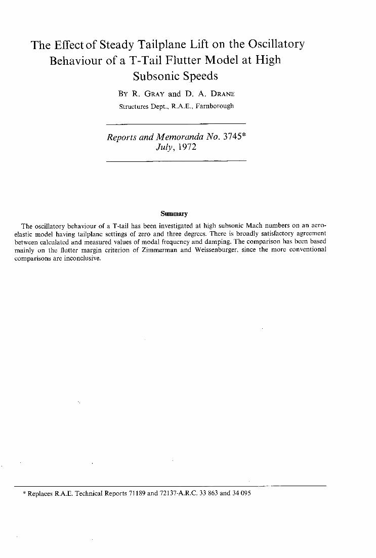
Reports and Memoranda No. 3745* July, 1972

Summary

The oscillatory behaviour of a T-tail has been investigated at high subsonic Mach numbers on an aero- elastic model having tailplane settings of zero and three degrees. There is broadly satisfactory agreement between calculated and measured values of modal frequency and damping. The comparison has been based mainly on the flutter margin criterion of Zimmerman and Weissenburger, since the more conventional comparisons are inconclusive.

* Replaces R.A.E. Technical Reports 71189 and 72137-A.R.C. 33 863 and 34 095

LIST OF CONTENTS

1. Introduction

2. Model and Test Rig

2.1. Model design and construction

2.2. Model support

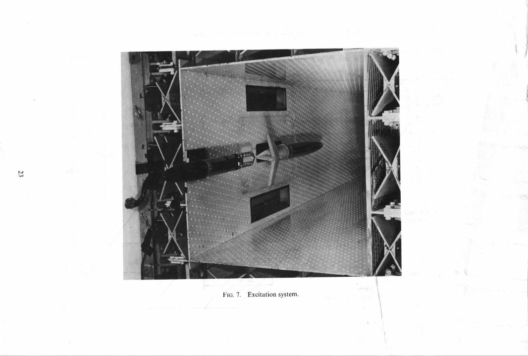
2.3. Excitation

2.4. Instrumentation

3. Response Measurements

3.1. Measurements in still air

3.2. Measurements in the wind tunnel

4. Calculation of Subcritical Response and Flutter Speed

5. Discussion

5.1. Test results and comparison with calculation

5.2. Flutter margin function

5.3. Improvements in test technique and analysis

6. Concluding Remarks

Acknowledgment

Appendix A

Appendix B

Tables I to 7

Derivation of oscillatory aerodynamic forces caused by steady lift on the tailplane

Derivation of the flutter margin function F

References

Illustrations Figs. 1 to 21

Detachable Abstract Cards

2

1. Introduction

The evaluation of the unsteady aerodynamic forces acting on a T-tail has in the past presented particular problems. 1'2'3 The publication by D. E. Davies 4 of a rigorous method for calculating the oscillatory aero- dynamic force inputs of a T-tail permits the antisymmetric flutter behaviour of these structures to be predicted when there is no steady lift on the tail plane. In practice, however, the vertical trimming forces exerted by the tailplane are rarely zero, and it has been shown 1'5 that the tailplane incidence can have a marked effect on the pattern of flutter behaviour. A method which includes additions to the theory of D. E. Davies has been devised which enables the flutter characteristics to be obtained for a tailplane at incidence.

The oscillatory behaviour of a T-tail aeroelastic model was previously investigated 5 at low subsonic wind speeds over a range of tailplane settings. The present report covers a similar programme of investigations the aim of which has been to confirm the validity of the current methods of calculating flutter behaviour at high subsonic speeds.

Wind-tunnel tests were made at high subsonic Mach numbers using a model of the T-tail of the hypothetical aircraft which had provided the basis for the low speed programme. 5 The tests consisted of exciting the model at a constant force level over a bandwidth of frequencies close to each resonance and making response measure- ments at speeds below the critical flutter speed, (the so-called steady-state method). The natural frequency and damping of the first three antisymmetric modes of the tail unit were determined from analysis of vector response diagrams. Test results were compared with calculated values of modal frequency and damping.

Two factors had a significant effect on the experimental part of the programme, and ultimately on the usefulness of the results. One of these was that a 'hard ' type of flutter was predicted for the system : that is to say, as the flutter condition was approached the damping in the critical mode fell very rapidly to zero over a small speed range. The other factor was that the wind tunnel in which the tests were made suffered from a degree of flow unsteadiness which subjected the models to high levels of forced response. Initially tests could not be made at Mach numbers below 0.85 and although subsequent development permitted testing at M = 0-7 flow unsteadiness resulted in the loss of three models and caused a high level of scatter in the results, especially near the critical flutter speed.

The objectives of the high speed programme have not been fully realised, but the information gathered does provide a measure of confidence in flutter prediction methods for T-tails at Mach numbers up to 0.90.

2. Model and Test Rig

2.1. Model Design and Construction The design of the models was based on a hypothetical aircraft which has also been the subject of a low speed

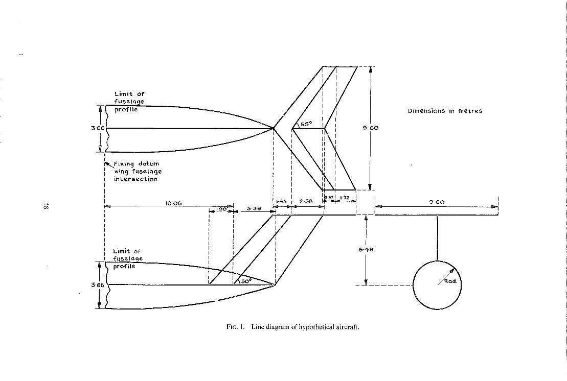
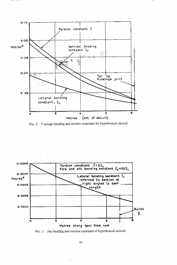
aeroelastic investigation. Tail flutter of this aircraft was assumed not to affect the forward fuselage and wings : therefore the model represented only the tail unit and aft fuselage, and was 'built-in' at the wing-fuselage intersection. The geometry and structural characteristics of the hypothetical aircraft are shown in Figs. 1 to 3 and its mass distribution is listed in Table 1.

The dimensional scale of the models was chosen so that the blockage of the wind tunnel was less than 1 percent of the cross-sectional area. The other main design conditions were that, at the flutter condition,

M,. = M. ,

f f rn __ ~Y a

P m P a

and

sm so pmV¢ poV '

where M = Mach number, a = structural density, p = air density, S = a structural stiffness parameter, V = air velocity

and the suffixes m and a refer to the model and the hypothetical aircraft respectively. The wind tunnel could

achieve the required values of V, and M,,, so it follows that for similarity

Sm Sa i O" m G a

i.e., the model should have the same structural efficiency as the hypothetical aircraft. The rear fuselage and fin were designed to satisfy this criterion: the tailplane, however, was made as stiff

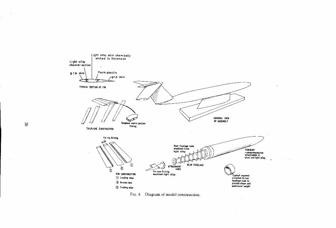
as possible by increasing the skin thickness over that appropriate to the similarity criteria so that the tailplane could be assumed rigid. There was then no need to take account of motion in symmetric modes in the analysis of flutter characteristics. An R.A.E. 101 aerodynamic section was chosen for the fin and tailplane : the thickness- to-chord ratio was 62 per cent. The tail surfaces were thinner than those employed on most current high- subsonic aircraft, but were adopted in an attempt to minimise aerodynamic thickness effects and also to facilitate exploration of the high-subsonic region.

Fig. 4 is a diagram of the model: it is illustrated in Figs. 5 to 7. All structural parts of the models were made from aluminium alloy stabilised where necessary by foam plastic.

The strength and stiffness characteristics of the fuselage were provided by a straight tapered tube with integrally machined stiffening rings: the walls of the tube were 0.39 mm (0-015 in) thick. The required mass distribution was achieved by attaching a series of rings made from G.E.C. heavy alloy. These were set into foam segments which provided the fuselage profile. A tail cone fitting bolted to the rear end of the filselage carried the tail unit and the permanent magnet which formed part of the excitation system.

One hazard of flutter testing is that premature failure can occur for reasons unconnected with flutter. As a precaution, three tail units having similar aeroelastic characteristics were built for these tests.

The fin of each unit consisted of a single cell metal box having skin and spar thicknesses of 0.078 mm (0.003 in). There were no intermediate ribs: skin and section stability were maintained by a plastic foam core.

The extremity of the fin box was closed by a fitting which carried the tailplane. This fitting also incorporated a simple jacking device which enabled the incidence of the tailplane to be varied.

The tailplane was built in two halves, which were joined by the central fitting. Each half was a two-cell box having skin thicknesses of 0-20 mm (0-008 in) and cores of plastic foam : there were no transverse ribs.

The profiles of both the fin and tailplane were completed by attaching leading and trailing edges. The outer surfaces of these were moulded in glass reinforced plastic 0-025 mm (0.001 in) thick filled with plastic foam.

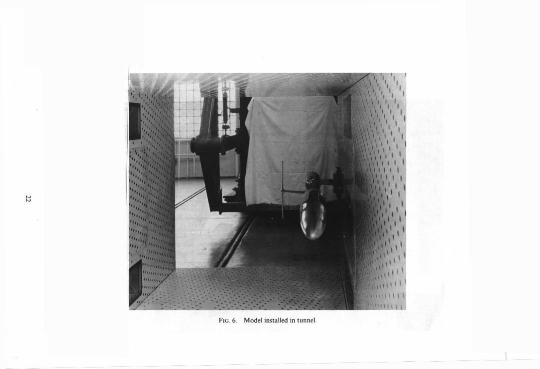
2.2. Model Support The method of supporting the models is illustrated in Figs. 4 to 7. The fore body was made from aluminium

alloy and faired into a steel centre section to which the model was attached. This assembly was strut-mounted from the wall of the R.A.E. 3 fl x 3 ft wind tunnel.

2.3. Excitation The model was oscillated laterally by an electro-magnet acting on the permanent magnet fixed in the tail-

cone fitting: a faired body, attached to the tunnel wall by a strut carried the electro-magnet. The arrangement is illustrated in Fig. 7.

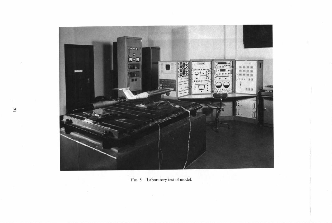
The current for driving the coil was obtained by amplifying the sinusoidal output of the decade oscillator in the ELVIRA equipment ~' (Fig. 5).

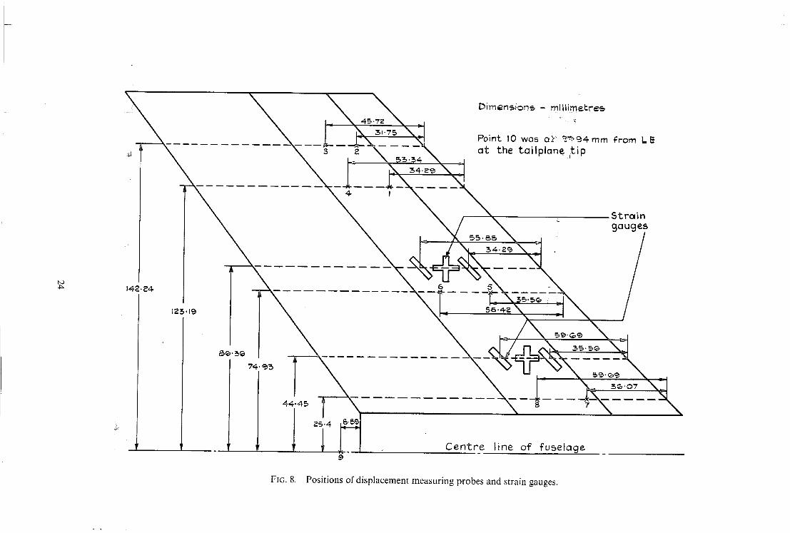
2.4. Instrumentation The response of the models in the wind-tunnel tests was sensed by strain-gauge bridges arranged to measure

fin bending-moment and torque (Fig. 8). The output of each bridge was fed directly to the ELVIRA equipment. Transducer signals were displayed as voltage measurements of the response in phase and in quadrature with the exciting force. These voltages were fed out to a Bryans X--Y plotter for direct drawing of the vector-response plots.

3. Response Measurements

3.1. Measurements in Still Air The modal shapes and resonance frequencies of the model in still air were obtained from measurements of

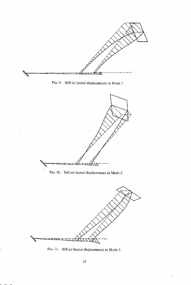
the displacement at the positions shown in Fig. 8 ; the mode shapes are shown in Figs. 9 to 11. Rolling motions of the tailplane were obtained by measuring displacements at the tailplane tip. These values were consistent with the assumption that the tailplane was rigidly attached to the top of the fin. Added mass tests were made to determine the direct inertias.

4

3.2. Measurements in the Wind Tunnel Two series of tests were made in the R.A.E. 3 ft × 3 ft wind tunnel using the perforated-liner working-

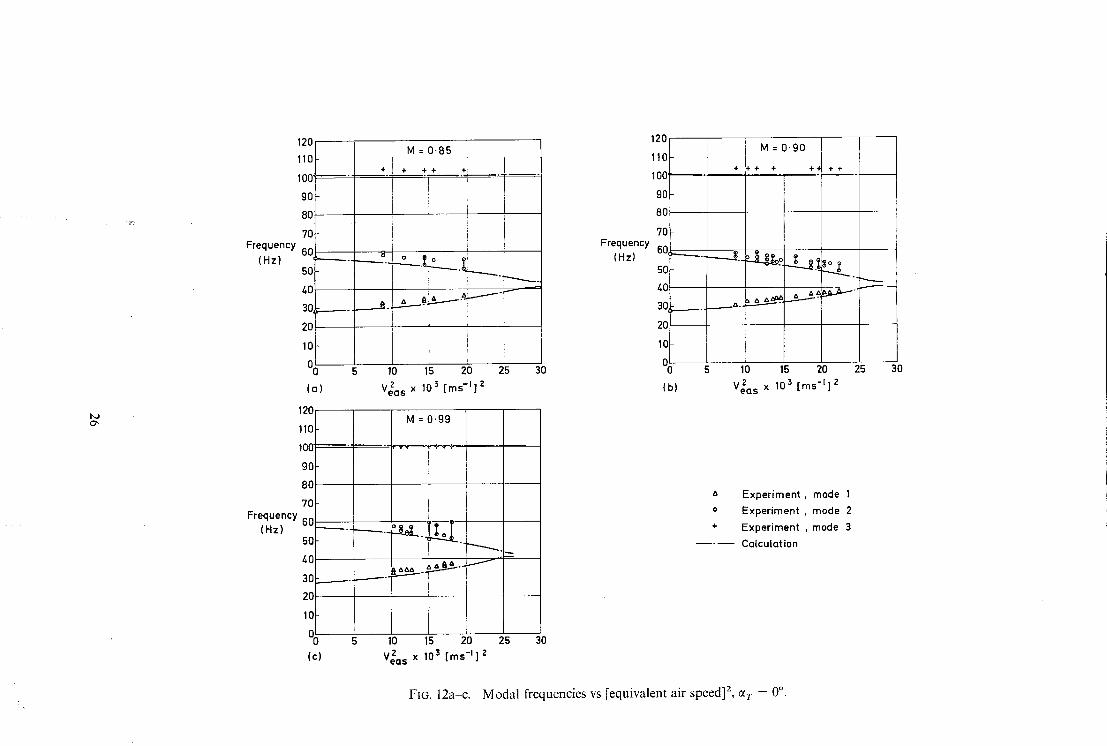
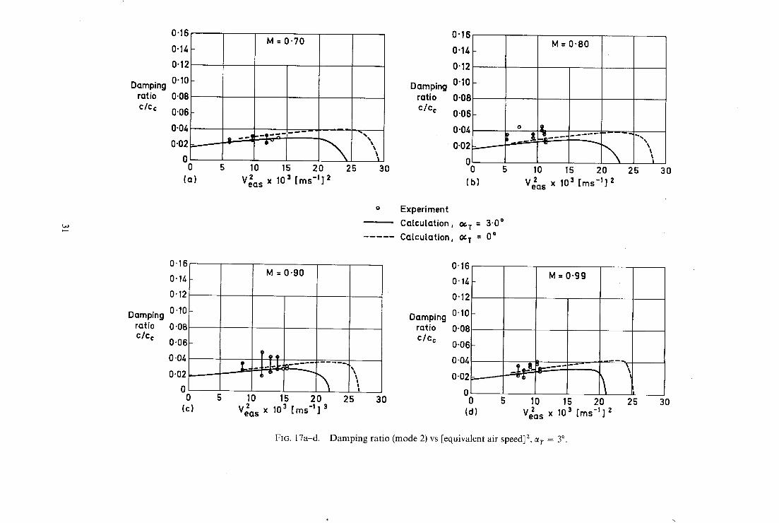
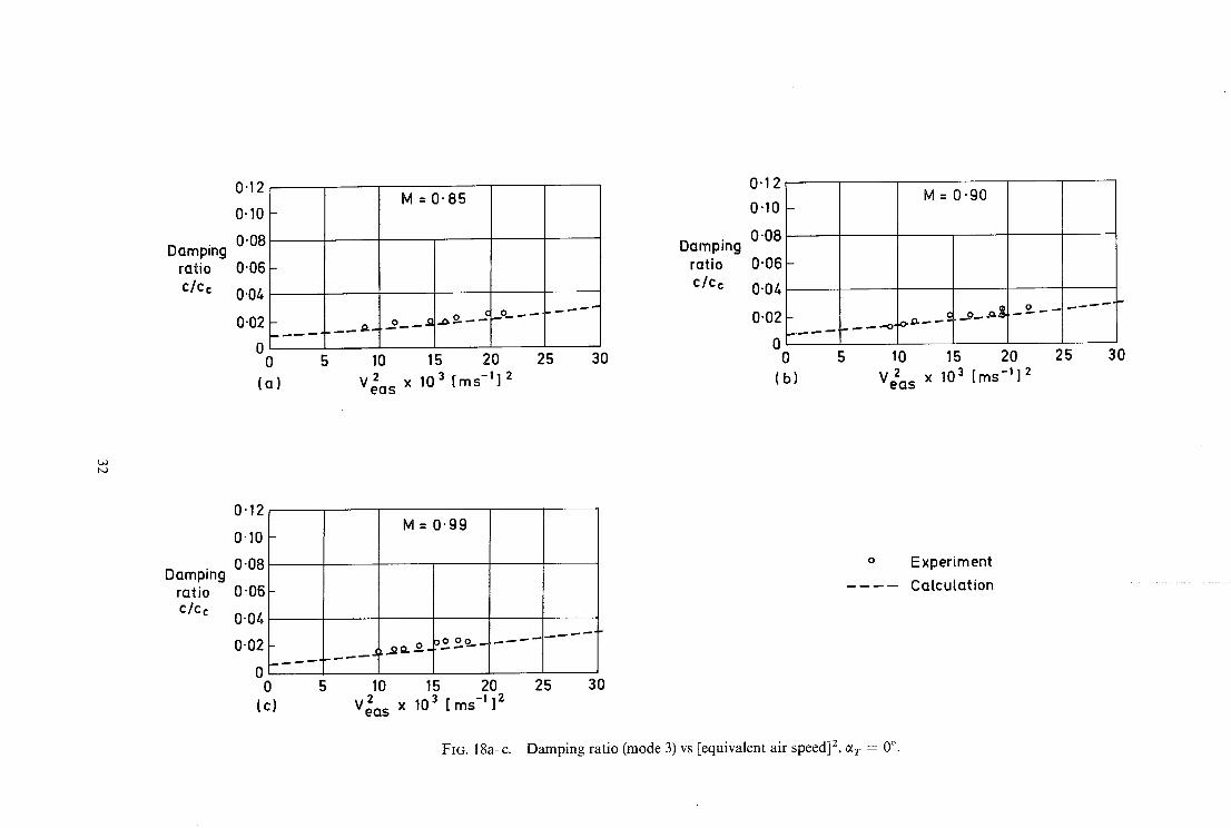
section. For the first tests the tailplane was set at zero degrees incidence and measurements taken at Mach numbers of 0.85, 0.90 and 0.99. During these tests the noise characteristics of the perforated-liner working- section were such that measurements could not be made at Mach numbers below 0.85. Subsequently, modifi- cations were made to the wind tunnel and the second series of tests were run with a tailplane setting of three degrees at Mach numbers of 0.70, 0.80, 0.90 and 0.99. The nominal frequency parameter at flutter, based on the fin and tailplane common chord, varied between 0.14 and 0-10 and the Reynolds number between 1.2 × 106 and 0-9 × 106. At each Mach number, and at a given setting of tunnel total pressure, the model was excited sinusoidally at a fixed peak force. The response from the strain gauges over the resonance bandwidths of the modes of interest was measured and recorded in the form of vector plots. The circles drawn on these were analysed to obtain the modal frequencies and damping ratios. The motions excited were fuselage and fin bending (mode 1) (see Fig. 9), fin torsion (mode 2) (see Fig. 10), and fuselage and overtone fin bending (mode 3) (see Fig. 11). The results of the tests are shown in Figs. 12 to 18 as graphs of the variation of modal frequen- cies and damping ratios with the square of the equivalent airspeed. The reasons for illustrating the results in this form are discussed in Section 5.2.

It had been hoped that any change in tailplane angle of incidence between wind-on and wind-off conditions might be determined from the response of the strain-gauge bridges mounted in the tailplane. However, the very poor signal to noise ratio precluded the taking of accurate measurements, and as no significant changes of level were observed, it was concluded that changes in incidence due to aerodynamic loading were small.

4. Calculation of Subcritical Response and Flutter Speed

Flutter calculations were based on the first three measured antisymmetric modes of the model. The mode shapes are illustrated in Figs. 9 to 11.

The inertia terms in the equations of motion were obtained from measured values of generalised mass, and if it is assumed that the measured modes are orthogonal, the inertia and structural stiffness coupling terms are zero. The direct stiffness terms were derived from the measured modal frequencies and inertias, whilst the structural damping terms were taken from the still-air damping measurements. The structural- damping coupling terms are assumed to be zero.

The zero-incidence aerodynamic terms in the calculation were derived from the D. E. Davies theory, 4 using modal displacements and slopes obtained from the measured modes. No allowance was made in the calculations for aerodynamic interference effects between the fin and the fuselage.

The equations of motion for the zero-degrees-incidence configuration of the model were solved for mode frequencies and damping. The calculations covered a range of aerodynamic conditions up to the critical flutter speed at each test Mach number. The results of the calculations are shown in Figs. 12 to 18, as graphs of the variation of frequency and damping ratio with (equivalent air speed) 2.

There are no rigorous methods for calculating the oscillatory aerodynamic forces on a T-tail in the condition where the tailplane produces steady lift. Therefore, as in Ref. 5, comparative flutter calculations were made by testing the aerodynamic-force inputs obtained from an equivalent zero-incidence condition and adding to them the inputs from;

(a) a lateral component of the lift force caused by angular displacement of the tailplane in roll, (b) a rolling moment caused by angular displacement of the swept tailplane in yaw, (c) a rolling moment caused by angular velocity of the tailplane in yaw, and (d) a rolling moment caused by lateral velocity of the tailplane.

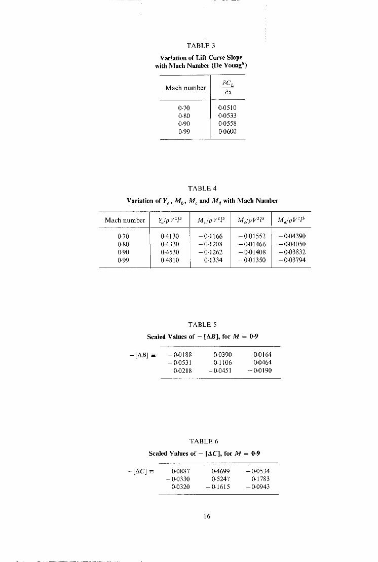
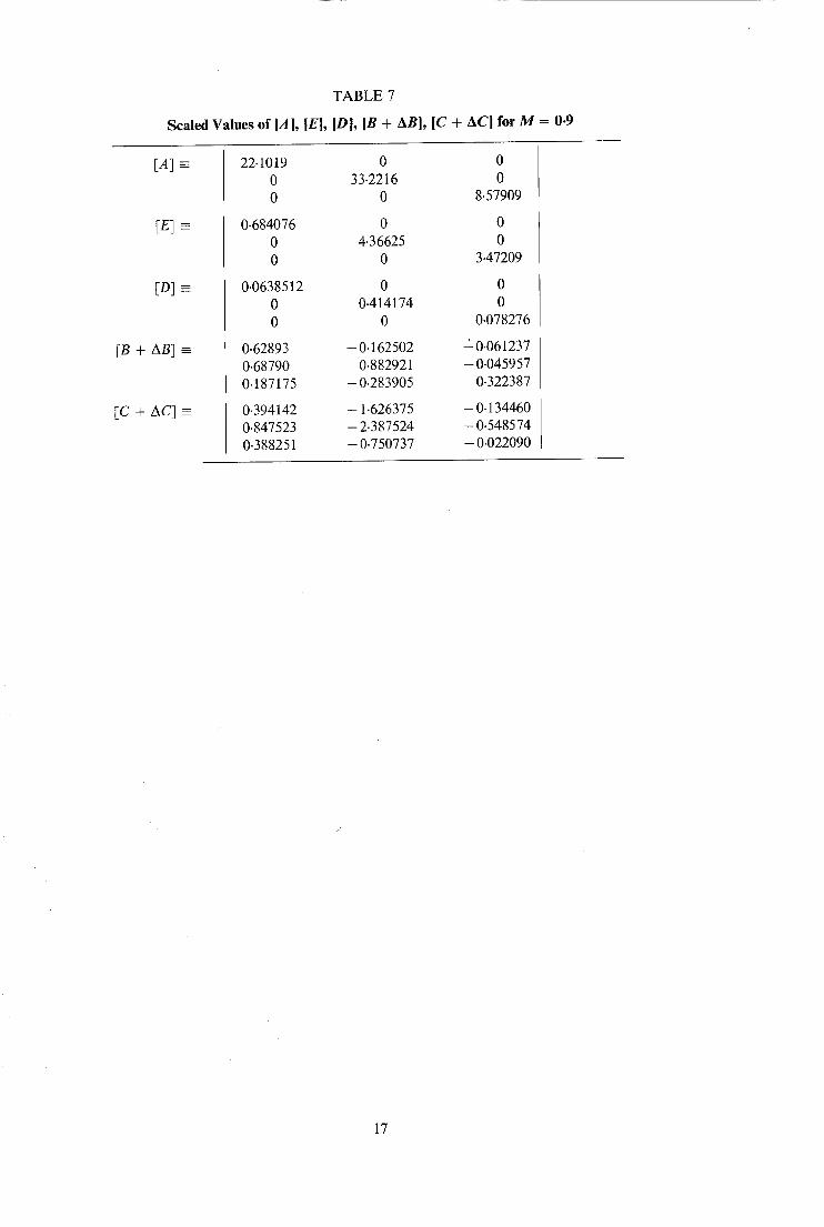
Terms (a) and (b) add to the aerodynamic stiffness and (c) and (d) to the aerodynamic damping. Measured modal displacements and slopes were used in calculating these terms. Fuller details of the procedure and the relevant quantities are given in Appendix A and Tables 3 and 4. Tables 5 and 6 list values of the additional terms and Table 7 gives a set of coefficients for the flutter equations at the condition M = 0-90.

5. Discussion

5.1. Test Results and Comparison with Calculation A general picture of the modal behaviour of the models (as airspeed is increased to the critical flutter con-

dition) can be obtained by an examination of the calculated characteristics shown in Figs. 12 to 18, which cover the Mach number and incidence ranges of the tests.

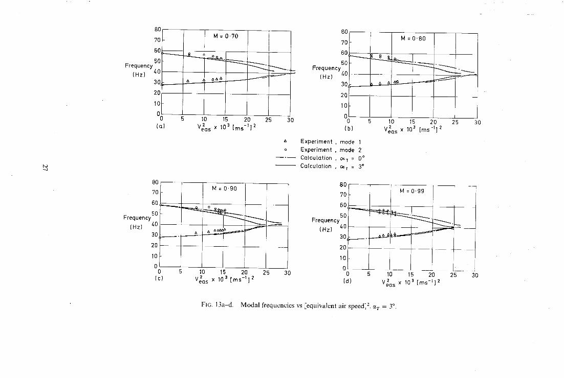
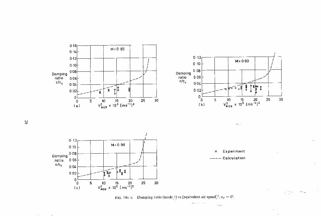
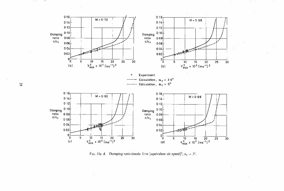
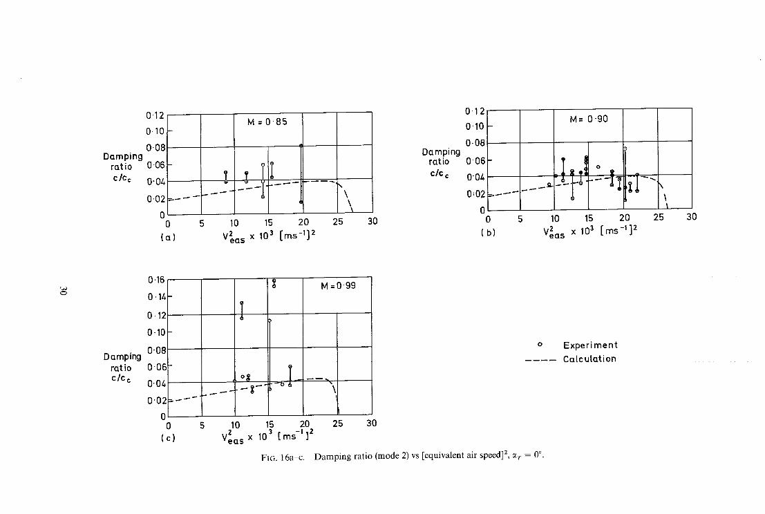
In general, the characteristics do not alter in pattern significantly as Mach number is increased. Figs. 12 and 13, which illustrate the calculated changes of modal frequency with airspeed, show that with both zero and three degree settings of the tailplane the frequency of the second mode falls and that of the first mode rises as the critical flutter condition is approached : the frequency of the third mode remains virtually invariant with speed. Figs. 14 to 17 illustrate the variation of modal damping ratio for the first two modes ; Figs. 14 and 15 show that the damping in the first mode rises steadily as speed is increased, the rate of damping increasing markedly close to the flutter speed. In Figs. 16 and 17 it can be seen that the damping in the second mode rises steadily to a maximum, then decreases very rapidly to zero at the flutter speed. The third mode damping ratio (Fig. 18) for the zero setting case, rises slowly and steadily as speed is increased, with no change in characteristic up to the critical speed. A similar pattern was observed in the three degree setting calculations. Indeed, the calculated characteristics for the three degree setting of the tailplane are broadly similar in pattern to those calculated for the zero setting configuration over seventy per cent of the zero setting critical speed range. Beyond this, frequencies and damping ratios change very rapidly with a three degree tailplane setting, and flutter occurs at a significantly lower airspeed.

The calculated rate of increase of damping in the first mode (Figs. 14 and 15) and the rate of decrease in the second mode (Figs. 16 and 17) as the critical flutter condition is approached, suggested that experimental verification of these trends would be very difficult to obtain--as proved to be the case. It is obvious that the calculated flutter speed can only be verified experimentally if damping in the second mode can be measured over the narrow range of speed just below the critical. The measurements have to be accurate if the flutter speed is not to be exceeded inadvertently, and the values of damping will necessarily be low, so that the model is increasingly sensitive to any disturbance such as tunnel turbulence. Moreover, since the method of measuring damping is by measuring the steady state response of the model to a sinusoidal force input over the frequency bandwidth of the mode, the accuracy of the damping values depends on being able to obtain consistent steady- state responses over the period during which the measurements are made. For the reasons outlined in Section 5.3, it proved impossible to obtain consistent response signals close to the flutter condition and in this region the values of damping ratio were inaccurate and there was a wide scatter in test results.

The first of the two models prepared for the tests was lost during tests close to the critical flutter condition. When these tests were conducted a characteristic of the turbulence in the perforated-liner section of the 3 ft × 3 ft tunnel was such that, at irregular intervals, models were subjected to a sharp input peak well above the mean level, and it was one such input that resulted in model failure.

To conserve the other models it was decided to avoid testing in conditions that might result in model overload and failure until the lower end of the speed range had been explored. This part of the programme for the zero tailplane setting had almost been completed when the second model was destroyed because of a wind-tunnel control failure. The third model, which was used to investigate the flutter behaviour with a three degree tailplane setting, successfully covered the low-speed part of the subcritical speed range, but failed in fatigue before exploration of the high sub-critical speed range could begin.

Against this background, we can now examine the experimental results, and their relationship with the calculations. Throughout the tests, the agreement between measured and calculated modal frequencies is good, as is shown in Fig. 12. At all three test Mach numbers the measured frequencies tend to be slightly higher than those calculated, but the differences are not large. The calculated trend towards frequency coalescence between the first and second modes is clearly seen in the experimental results.

The measured dampings in the first mode (Fig. 14 and 15) fall somewhat below the calculated values, and in particular, the measured values do not increase with airspeed to the extent that calculation indicates. Damping in the second mode is, of course, the most important parameter to be measured in the tests, because its value is a direct guide to the approach to the critical flutter condition. Figs. 16 and 17 show the measure of agreement between experiment and calculation. In general the measured values are above the calculated ones, and have a tendency to increase with speed at a higher rate. However, the scatter of the results is indicative of the test difficulties, and also of the problems faced in trying to decide whether an incremental speed increase could be made without hazarding the model. If for example in Fig. 16a the lower of the damping values at the highest speed is to be believed, then an increase in speed to V~a ~ = 150 m/s could result in flutter, if the model follows the calculated trends. At M = 0.90 (Fig. 16b) a clear-cut reduction in the damping of the second mode with speed is evident: the damping values measured at this Mach number were again higher than calculated over the lower end of the speed range.

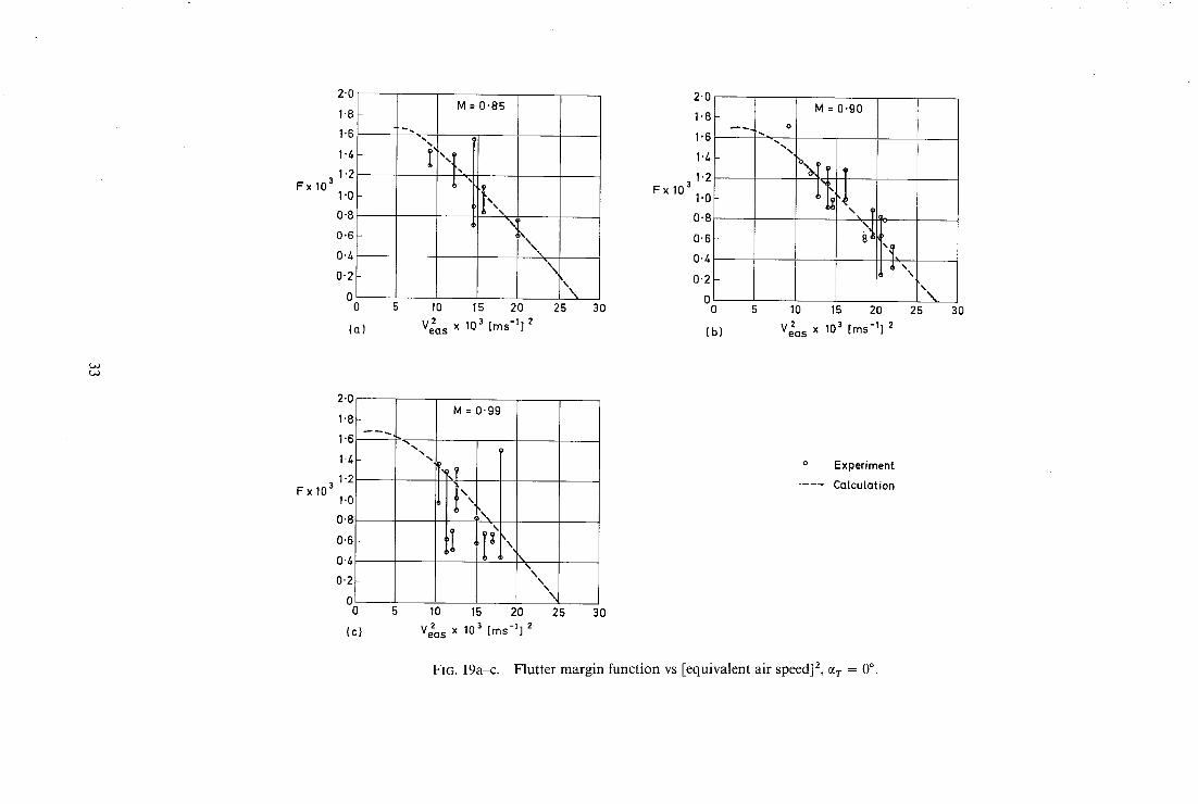
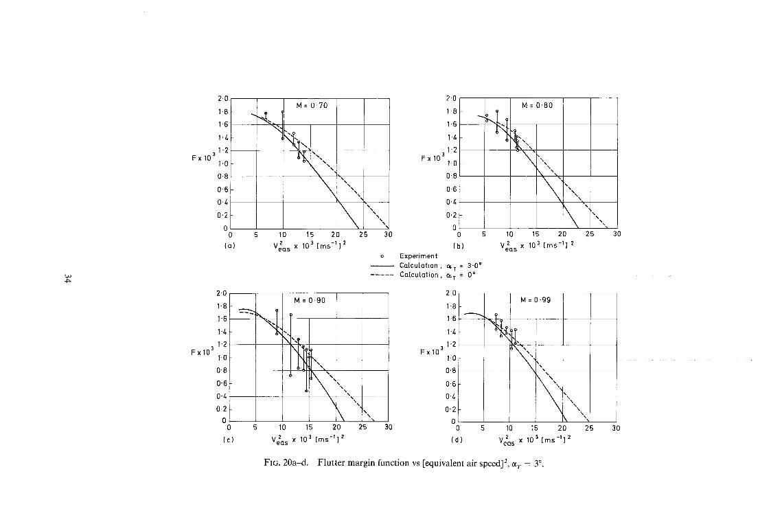
5.2. Flutter Margin Function In view of the unsatisfactory nature of the experimental results in providing a measure of the critical flutter

speed from the damping trends, both the calculated and experimental data were analysed in the form of the

6

flutter margin function,~proposed by Zimmerman and Weissenburger in 1963. 7 The function is applicable to binary systems and takes the form of an expression which is dependent on the frequevcy and damping of the two modes involved. The value of the function is positive at speeds below the critical, and zero at the critical flutter speed. The advantage of using the function (which is called by Zimmerman and Weissenburger the 'flutter margin') is that its value decreases smoothly with increasing speed right up to the flutter speed; this is in marked contrast to curves of modal damping which may vary very rapidly both in slope and in value close to the flutter speed. The main disadvantage of using the flutter-margin function is that it is strictly applicable only to a binary system, although it is stated that methods of using it with multi-degree-of-freedom systems have been developed and used. In the investi~ati'on described here, the calculations had shown that the inclusion of mode 3 had only a small effect on the flutter and subcritical response characteristics, so that the system could be regarded as an effectively binary system involving modes 1 and 2. An outline of the derivation of the function is given in Appendix B.

The calculated and experimental results of Figs. 12 to 18 are plotted in terms of the 'flutter margin', F, in Figs. 19 and 20. It can be seen that the calculated results give a smooth variation in F; moreover, when F was evaluated for modes 1 and 2 using theoretical data for both series of tests, flutter speeds were obtained

close to those given by the'~r-nary~nalysis. In the zero setting cases (Fig. 19) the experimental which are very results, although having considerable scatte',r~d¢follow" r the calculations reasonably closely at M = 0.85 and M = 0.90, and indicate a flutter speed somewhat lower than calculated at M = 0.99. Fig. 20 shows that the differences in calculated values of F between the zero and three degree tailplane settings can be detected at a lower proportion of the flutter speed than can the differences in either the frequency or damping ratio alone. Despite the limited speed range covered in the three degree settings tests, and despite a degree of scatter, the experimental trends at M = 0.70, M = 0-80 and M = 0.90 follow the calculated curve. Results at M = 0-99 are conflicting; those from tests at zero settings indicate a lower than calculated flutter speed, whereas those from tests at three degrees of incidence suggest that flutter may not occur so soon as calculation indicates.

In an earlier investigation at M = 0.10, flutter speeds calculated on the basis of the procedure used in the present tests, agreed well with measurements. Enough additional information has been gathered in the present tests to provide a measure of confidence in the method of calculating flutter behaviour at high-subsonic Mach numbers.

5.3. Improvements in Test Techniques and Analysis The difficulties of obtaining consistent experimental test results have been made clear in the previous

sections and give rise to two questions. Why are the test results given in this Report apparently of poorer quality than some of those obtained in other and similar tests in the same wind tunnel, and how can techniques be improved? A partial answer to the first question may be that the modal frequencies of the T-tail models lay well below the frequencies of other models, making this model more susceptible to the transient flow dis- turbances that occurred throughout the tests. For example, an (unpublished) set of test results from an aero- elastic model of a specific aircraft, tested in the R.A.E. 3 ft x 3 ft tunnel, gives values of modal damping that follow smooth curves almost to the critical flutter speed, and with little scatter. However, for that model, the lowest mode frequency was above 100 Hz, and the modes of interest had frequencies up to 400 Hz. It may be noted that mode 3 of the T-tail models (having a still air frequency of 101 Hz) invariably gave consistent vector- response curves which presented no difficulty in analysis.

Despite the provision of signal analysis equipment which was insensitive to signal components differing in frequency from that of the sinusoidal input, the large amplitude generated by the transient flow disturbances, particularly in mode 1, resulted in signal-to-noise ratios which were too small to be handled satisfactorily. A further difficulty arose from the change of behaviour of the model in mode 2 when the wind was turned on. In still air the vector plots obtained were perfectly acceptable, but with wind on the signal-to-noise ratio from the set of gauges intended to sense this motion was barely sufficient to permit operation of the equipment, even when the model was excited to amplitudes at which serious fatigue damage might have been expected. Indeed, signal-to-noise ratio diminished so rapidly when the wind was turned on that it seems possible that the modal shape (see Fig. 10) changed sufficiently to reduce drastically the outputs of the strain gauges.

Where flutter tests have to be made in tunnels which have unsteady flow characteristics, it is a requirement that the test technique should enable measurements to be obtained that are independent of the flow disturbances. The current U.K. technique of obtaining vector plots from the steady-state forced response, at a number of discrete frequencies for each mode of interest, does not meet this requirement. Tests with current analogue equipment can demand signal-to-noise ratios which are only obtainable at levels of excitation which pose fatigue problems for the model; additionally they are very time-consuming. The improvements offered by digital analysis of response data, and in particular by the use of on-line fast Fourier transform facilities appear

to be very considerable, both in improving the quality of test results, (even in 'noisy':,tunnel conditions) and in speeding up the whole test process. It is felt that development of these techniques for application in wind- tunnel flutter tests should be pursued as soon as possible.

6. Concluding Remarks

High-speed wind-tunnel tests have been made to measure the subcritical response of an aeroelastic model of a T-tail using two tailplane settings. The test results have been compared with theory which makes use of the methods of D. E. Davies and which also takes into account terms which are proportional to steady lift forces on the tailplane.

Whilst agreement between theory and experiment, based on measurements of frequency and damping ratio, was generally satisfactory within acceptable limits of experimental error, the model failed before any measure- ments could be made in the immediate subcritical speed range in which large and significant changes in modal characteristics occur. Moreover, scatter in the available measurements made interpretation difficult. In these circumstances the flutter margin criterion of Zimmerman and Weissenburger which takes account of both modal frequencies and dampings proved a more satisfactory basis for comparison. Theoretical trends of flutter margin are followed reasonably closely by experiment between M = 0-70 and M = 0.90.

An earlier investigation in this series has shown that the theory gives good estimates of subcritical response and flutter speed over a range of incidences at M = 0.10. The present experiment has gathered sufficient additional information to provide a measure of confidence in the method of calculation up to a Mach number of 0-90.

Acknowledgment

The authors wish to thank the staff of the Structures Department Aeromodelling Laboratory who built the models used in these tests. They also acknowledge the great help given by Mrs. Irene Levett and Miss P. K. New, and by the tunnel operating services of Aerodynamics Department, R.A.E.

No. Author(s)

1 J .C .A . Baldock . .

2 S.A. Clevenson and S. A. Leadbetter

3 N.S. Land and A. G. Fox ..

4 D .E . Davies . . . . . .

D. J. McCue, D. A. Drane and R. Gray

6 W . D . T . Hicks . . . .

7 Norman M. Z immerman and J. T. Weissenburger

8 J. de Young and C. W. Harper

REFERENCES

Title, etc.

. . Determination of the flutter speed of a T-tail unit by calculations, model tests and flight flutter tests.

A.G.A.R.D. Report 221 (1958).

Measurement of aerodynamic forces and moments at subsonic speeds on a simplified T-tail oscillating in yaw about the fin mid-chord.

N.A.C.A.T.N. 4402 (1958).

. . An experimental investigation of the effects of Mach number, stabilizer dihedral and fin torsional stiffness on the transonic flutter characteristics of a tee-tail.

N.A.S.A.T.N. D-924 (1961).

. . Generalised aerodynamic forces on a T-tail oscillating harmoni- cally in subsonic flow.

A.R.C.R. & M. 3422 (1964).

The effect of steady tailplane lift on the sub-critical response of a T-tail flutter model.

A.R.C.R. & M. 3652 (1968).

•. A control and measurement system for aeroelastic model tests. A.R.C.C.P. 1045 (1968).

Prediction of flutter onset speed based on flight testing at sub- critical speeds.

Paper at A.I.A.A./A.F.F.T.C./N.A.S.A.-F.R.C. Conference on testing of manned flight system.

Edwards Air Force Base, December 4-6 1963.

.. Theoretical symmetric span loading at subsonic speed for wings having arbitrary planform.

N.A.C.A. Report 921 (1950).

A P P E N D I X A

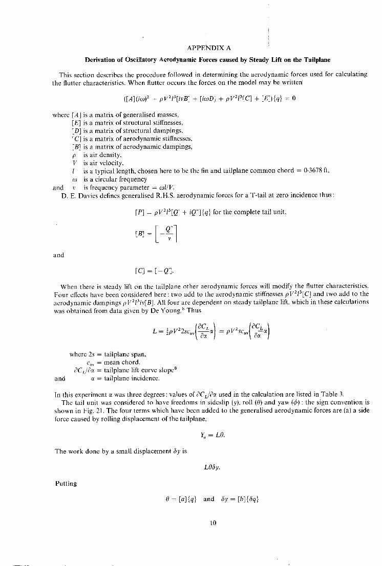
Derivation of Oscillatory Aerodynamfic Forces caused by Steady Lift on the Tailplane

This section describes the procedure followed in determining the aerodynamic forces used for calculating the flutter characteristics. When flutter occurs the forces on the model may be written

([A](ico) 2 + pV213[ivB] + [icoD] + pV213[C~ + [E]){q} = 0

where

and D.

[A] is a matrix of generalised masses, [E] is a matrix of structural stiffnesses, ED] is a matrix of structural dampings, EC] is a matrix of aerodynamic stiffnesses, [Bl is a matrix of aerodynamic dampings, p is air density, V is air velocity, l is a typical length, chosen here to be the fin and tailplane common chord = 0.3678 ft, co is a circular frequency v is frequency parameter = col/V.

E. Davies defines generalised R.H.S. aerodynamic forces for a T-tail at zero incidence thus:

[P] = pV213[Q ' + iQ"] {q} for the complete tail unit,

and

[c3 = E - Q'3.

When there is steady lift on the tailplane other aerodynamic forces will modify the flutter characteristics. Four effects have been considered here: two add to the aerodynamic stiffnesses pVZl3[C] and two add to the aerodynamic dampings pVZl3iv[B]. All four are dependent on steady tailplane lift, which in these calculations was obtained from data given by De Young. s Thus

l 2 IOCL \ z IOCL \

and

where 2s = tailplane span, Cav = mean chord,

?CL/&~ = tailplane lift curve slope 8 c~ = tailplane incidence.

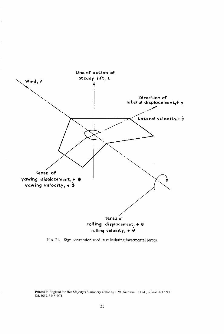
In this experiment e was three degrees ; values of ?CL/&~ used in the calculation are listed in Table 3. The tail unit was considered to have freedoms in sideslip (y), roll (0) and yaw (qS) : the sign convention is

shown in Fig. 21. The four terms which have been added to the generalised aerodynamic forces are (a) a side force caused by rolling displacement of the tailplane,

Ya = LO.

The work done by a small displacement @ is

LO6y.

Putting

0 = [a]{q} and 6 y = [b]{6q}

10

then

Thus

Ya6y = [6q]r[b]r(L)[a] {q} - pV213[6q]r[AQ'.] {q}, say.

L AQ; =p--~--~[b]r[a],

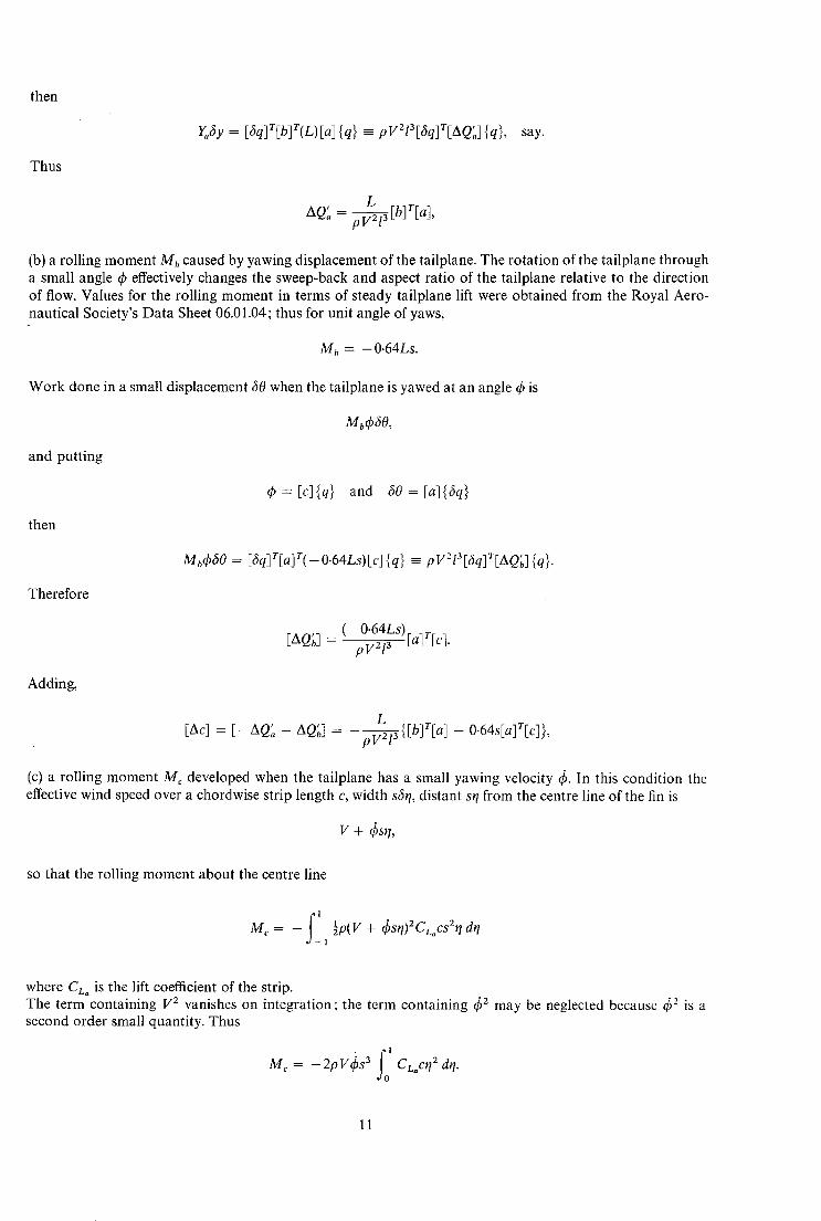
(b) a rolling moment M b caused by yawing displacement of the tailplane. The rotation of the tailplane through a small angle ~b effectively changes the sweep-back and aspect ratio of the tailplane relative to the direction of flow. Values for the rolling moment in terms of steady tailplane lift were obtained from the Royal Aero- nautical Society's Data Sheet 06.01.04; thus for unit angle of yaws,

M b = - - 0 . 6 4 L s .

Work done in a small displacement 60 when the tailplane is yawed at an angle q~ is

and putting

then

Therefore

Mb~b60,

qS= [c]{q} and 30 = [a]{aq}

Mb49bO = [6q]T[a]T(--O'64Ls)[c] {q} ---- pV213[aq]T[AO'b] {q}.

(-0.64Ls)~ "~Tr 1 [AQ; ] - ~ LaJ [cj.

L [Ac] = [ -AQ' a - AQ~,] = pV2l 3 {[b]r[a] -- 0.64s[a]T[c]},

Adding,

(c) a rolling moment M c developed when the tailplane has a small yawing velocity ~. In this condition the effective wind speed over a chordwise strip length c, width s&/, distant sq from the centre line of the fin is

so that the rolling moment about the centre line

V + ~sr/,

f l

M~ = - ½p(V + ~)S~)2CLaCS2?] dq - 1

where CLa is the lift coefficient of the strip. The term containing V 2 vanishes on integration; the term containing 4~ 2 may be neglected because ~2 is a second order small quantity. Thus

M~ - 2p V~os 3 I'|l = CLaCt] 2 drl. 3o

11

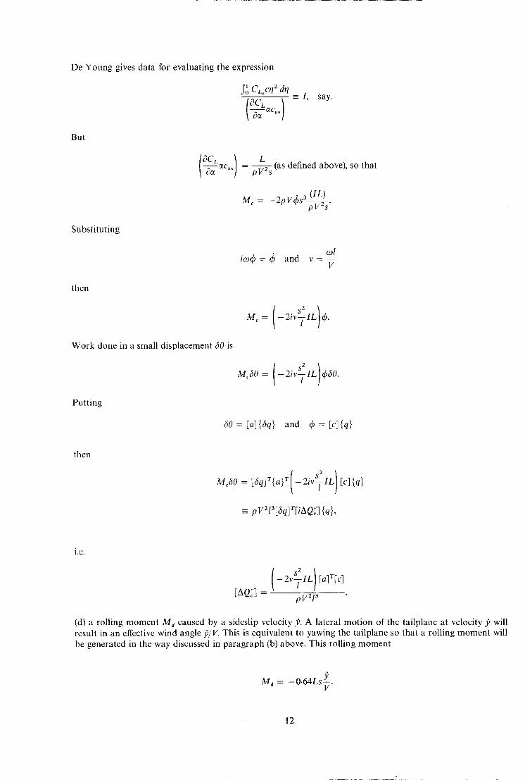
De Young gives data for evaluating the expression

2

But

Substituting

then

Work done in a small displacement (30 is

Putting

say.

~Cav = ~ (as defined above), so that

M~ = - 2 p V $ s 3 (IL) pV2s"

ico~b=q~ and v = - - V

( s2) M~ = - 2 i v ~ l L qS.

s2 IL) 4)(30. McaO = ( - -2 ivy

(30= [a]{(3q} and qg= [c3{q}

then

Me(30 = [3q]T{a} T - 2 i v T I L [c]{q}

-- pV213[~Sq]r[iAQ'~] {q},

i.e.

( s2) - 2 v T I L [a]m[c]

[AQ;'] = py213 ,

(d) a rolling moment M a caused by a sideslip velocity p. A lateral motion of the tailplane at velocity .P will result in an effective wind angle y:/V. This is equivalent to yawing the tailplane so that a rolling moment will be generated in the way discussed in paragraph (b) above. This rolling moment

Me = - 0.64LsY.

12

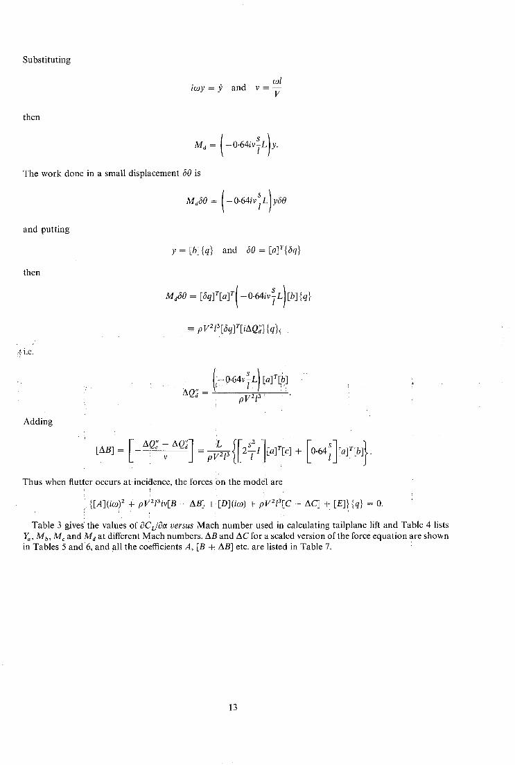
Substituting

col icoy= .9 and v = - -

V

then

Ma = -0.64iv~L y.

The work done in a small displacement 80 is

064+),0 and putting

y = [b]{q} and a0 = [a]r{aq}

then

Ma60 = [aq]r[a]r( --O'64iv~ L)[b] {q}

= p V213[bq]W[iAQ'~] {q}~

.< i.e.

AQ:; =

; ~ S (.oo4v L) alT ! pV213

Adding

[ ] {is2] [0 } [AB] = ~0;' AQ~ :L 2 7 I [a]T[c] + .64 [a]rE b] : V pV2l 3

Thus when flutter occurs at incidence, the forces on the model are f : ,! , '.

{[A](ico) z + pV213iv[B + AB] +:[D](/co) + pv2ta[c + AC] -F [E]} {q/ = 0. ! i i : .

Table 3 gives the values of ~?CL/~a versus Mach number used in calculating tailplane lift and Table 4 lists Y~, Mb, Mc and M a at different Mach numbers. AB and AC for a scaled version of the force equation are shown in Tables 5 and6, and all the coefficients A, [B -h AB] etc. are listed in Table 7.

'13

APPENDIX B

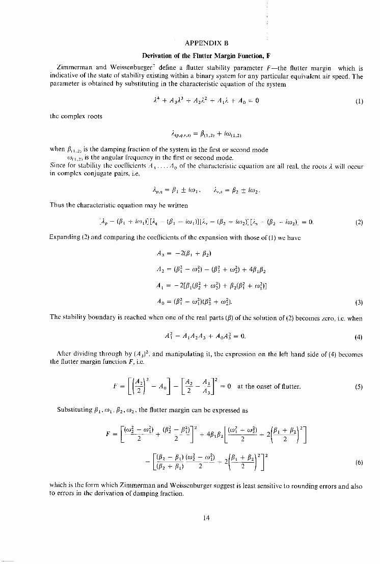
Derivation of the Flutter Margin Function, F

Zimmerman and Weissenburger 7 define a flutter stability parameter F- - the flutter margin--which is indicative of the state of stability existing within a binary system for any particular equivalent air speed. The parameter is obtained by substituting in the characteristic equation of the system

the complex roots

24 + A323 + A2 ~2 -+- Ax2 + A0 = 0 (1)

~(p,q,r,s) = fl(1,2) -[- io)(1,2)

when/~(~,2) is the damping fraction of the system in the first or second mode t:hl.2) is the angular frequency in the first or second mode.

Since for stability the coefficients A 3 . . . . A o of the characteristic equation are all real, the roots 2 will occur in complex conjugate pairs, i.e.

2p,q : f l l ----- i~01, J ' r , s : f12 ~ ioJ2"

Thus the characteristic equation may be written

[2p - - ( i l l + i ~ 1 ) ] [ )~ - - ( i l l - - i~° l ) ]E '~r - - (fi2 + im2) ] [)-~ - - (f12 - - h:o2)] = 0. (2)

Expanding (2) and comparing the coefficients of the expansion with those of (1) we have

A 3 = - 2 ( f l l + f12)

A, = -2[/~,(t~ + ,o22) + /h l /~ + ~,~)J

Ao = i/~ + ~o~)(/3~ + ~ ) . I3)

The stability boundary is reached when one of the real parts (/~) of the solution of (2) becomes zero, i.e. when

A 2 - A I A z A 3 + Ao A2 = O. (4)

After dividing through by (A3) z, and manipulating it, the expression on the left hand side of (4) becomes the flutter margin function F, i.e.

F = - Ao - A~l = 0 at the onset of flutter. (5)

Subst i tut ing/~, co 1 ,/~z, ~2, the flutter margin can be expressed as

~ + ~ ) ~ + a (6)

which is the form which Zimmerman and Weissenburger suggest is least sensitive to rounding errors and also to errors in the derivation of damping fraction.

14

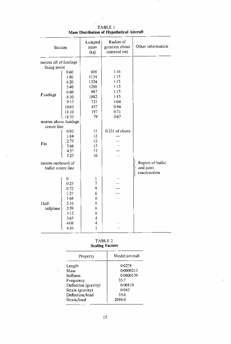
TABLE 1 Mass Distribution of Hypothetical Aircraft

Station

metres aft of fuselage fixing point

0.60 !-80 4.20 5.40 6.60

Fuselage 8.10

9.15 10.05 11.10

, 11.55 metres above fuselage

centre line 0-92 1.84 2.75

Fin " 3.66

4.57 5.25

metres outboard of bullet centre line

0 0.25 0.72 1.27 1.68

Half- 2.16 tailplane 2.59

3.12 3.65 4.08

, 4.56

Lumped mass (kg)

608 1134 1324 1288 987

1082 721 457 197 79

Radius of gyration about

centroid (m)

1-16 1-15 1-15 1.15 1.15 1.15 1.04 0.84 0.71 0.67

Other information

15 0.231 ofchord 12 12 13 12 16

1 7 9 6 6 6 6 6 4 4 1

Region of bullet , and joint

construction

TABLE 2 Scaling Factors

Property M odel/aircraft

Length Mass Stiffness Frequency Deflection (gravity) Strain (gravity) Deflection/load Strain/load

0.0278 0.0000213 0.0000139

35.7 0.00119 0.043

55.6 2010.0

15

T A B L E 3

Variation of Lift Curve Slope with Mach Number (De Young s)

Mach n u m b e r

0.70 0.80 0"90 0'99

~C L 0~

0.0510 0.0533 0-0558 0.0600

T A B L E 4

Variation of Y., Mb, Mc and M a with Mach Number

Mach number Ya/pV213 Mb/pV213 Mc/pV213 Md/pV213

0.70 0-80 0-90 0-99

0.4130 0.4330 0-4530 0-4810

- 0 . 1 1 6 6 - 0.1208 - 0 . 1 2 6 2 - 0 . 1 3 3 4

-0 .01552 -0 -01466 -0 -01408 -0 .01350

-0 -04390 -0 -04050 -0 -03832 -0 -03794

TA B LE 5

Scaled Values of - [AB], for M = 0-9

- lAB] = - 0 . 0188 0.0390 0.0164 -0 .0531 0-1106 0-0464

0.0218 -0 .0451 -0 -0190

T A B L E 6

Scaled Values of - [AC], for M = 0.9

- [AC] - 0-0887 0.4699 - 0-0534 - 0.0330 0.5247 0-1783

0.0320 - 0 .1615 -0 -0943

16

T A B L E 7

ScaledValuesoflAl, lEl, lDl, lB + AB], [C + A C I ~ r M = 0.9

[ A ] -

[B + AB] -

[C + AC] =

22.1019 0 0 0 33.2216 0 0 0 8-57909

0.684076 0 0 0 4.36625 0 0 0 3.47209

0.0638512 0 0 0 0.414174 0 0 0 0.078276

0.62893 -0-162502 ±0-061237 0.68790 0.882921 -0.045957 0.187175 -0.283905 0.322387

0.394142 - 1.626375 -0.134460 0.847523 - 2.387524 -0.548574 0-388251 -0.750737 -0.022090

17

T I :3'66

Oo

L i m i t of f u s e l a g e

prof i I¢

~,,, Fixin 9 do tum i win 9 f us¢ lQg¢ I I i n t e r s e c t i o n

3-66

L ' lmi t o f { u~¢ lag¢ p ro f i l e

10"06

I

1 1/

,'5"39 1-45

=t ~\ \ \", ! \ \ X \

Ii I "4\I \ , i i I

i I I

5-4oj

_l

Dimens ions in m e t r e s

9 - 6 0 I

I

FIG. 1. Line d iagram of hypothet ical aircraft.

0"10

0"08

Metres 4

O'OG

/

Torsion constant 3" /

bending Iv

'Oiio

O'; o~: i Lateral ~ bending l

constant , IL

FIG. 2.

2 4

Metres (aft of datum)

Fuselage bending and torsion constants for hypothetical aircraft.

8

0 . 0 0 0 5

0 . 0 0 0 4

M e t r e s ¢

0-0003 I

0"0002

o-oooi

O

FIG. 3.

Torsion constant, J = ZI L fore an~ a f t bending constant JF=~.SI.

~ La~er=l bending constant IL reCerred t o secL~on at

right, angles to spar

2 4 G 8

Met re s a l a n 9 spa r From root

Fin bending and torsion constants of hypothetical aircraft.

19

F~ C~

Light alloy skin chemically t etched to thickness

Light alloy I channel section\ i

g r p skin\ I Foam plastic ~ p skin

TYPICAL SECTioN OF FIN

/ ~ GENERAL VIEW / / / / :~ ~ c~, ~'. ,t~,...'*~..~ .. OF ASSEMBLY LJ ~ Tallploee centre section.

fitting TAILPLANE CONSTRUCTION

tip fitting.

FIH CONSTRUCTION Leading edge

~) Torsion bOX (~ Trolling edge

machined Irrom ~ \ _ ~ FONEBOOY

steel and light alloy

ATTACHMENT REAR FUSELAGE ~ T y CON E

Fin root fitting machined light alloy, piaol segment

attached to rear fuselage tube to provide shape and additional welghl.

FIG. 4. Diagram of model construction.

tO

FIG. 5. Laboratory test of model.

I',,.)

i I ' I i ' II

I I I I I *O |q l i l l

I !

l l l l

i l ' 0 ! g i

I I l

|1111 I f j g

' I f | I

P l lg~

I I l ~ l ,g

g lOIgq I 0 0 ~ | Q

I

# ! 1 1 1 t I I # 1 t !

I . I I #1

, ~- . ,,,~

. . . . ~.~l l . " .. ". -. - " ~ ~ |111111111111 , . . . - | r # | # l lO | I . " " . " "_ . . " ° - . .

. , , , . - . . \ " ._ . - . . . - . . . - . - . - . - . . - -

. ..-~.~ ".. '_..

FIG. 6. M o d e l installed in tunnel.

f d I ! ! i t! I I t , ~l I I I I I ~ * I t I I iJl ~ I I i p p I t ~ I t I I I I I tl I l

~l~ I I I I I i i t I

lllll II II I I

I I I i i i i i i i i i i I | l I I

I t 1 1 1 I t t l I t I I I t

t t 111 |

I I 11 | t I t t

I i 1 1 t I t i I

I i I t

I I i l l I

: : , i ! !

l

' '!r$

~ 1.2, -.

~-.

FIG. 7. E x c i t a t i o n s y s t e m .

4~ 14~.84

1~5,19

+ e . ~ e I 74, ~5

. . . . N - +

~ + L - ~" ++

~5.4

4 4 . 4 5

D i m e m ~ i o n ~ - m l t l i m s ~ r e ~

P o i n t 10 w a s o'-," ~ " 9 4 rnm ~ r o m I. a t the tai lplane t ip

,~ Strain

g o u g e s ~ . ~ \ _, I

/ \ - , ~-+°.+++,,,, +.

I+ ",~. - +o.o, \ _ . , ~ - ~ +~- \

Cent re line of fuselage 9

FIG, 8. Positions of displacement measuring probes and strain gauges.

\

,%

/

/ /

FIG. 9. Still air lateral displacements in Mode 1.

/

~ ~-~-~-~. . .~ FIG. 10. Still air lateral displacements in Mode 2.

FIG. 11. Still air lateral displacements in Mode 3.

25

l'-J

120

110

100

90

80

70 Frequency 60

(Hz) ' - - w-,___, ._ . .

50

40

30,

20

10

o; la )

120

110

100'

Frequency (Hz)

90

80

70

M = 0"B5

4" ÷ + + 4

8 o s o i

10 15 20

VgQs x 10 3 [ m s - I ] z

M =0 -99

J j - f

25

6o ~ ~ o

50 .-

4O

3 0 ~ _ _

20

10

% 5 10 15 20 25

(c) VeZas x 103 [ms - I ] z

30

30

120

110

100'

90

80

70 Frequency

(Hz) 60,

5O

40

30 ....

20

10

o; Ib}

M = 0-90

÷ + ÷ + + 4 + +

~ ~ - ~ - ~ ~ - ' ~ " ~

10 15 20 25

Ve2as x 10 3 I res - l ] 2

A Expe r imen t , mode 1

o Expe r imen t , mode 2

+ Exper iment , mode 3

m . _ _ Catculat ion

30

FIG. 12a-c . M o d a l f requencies vs [ equ iva len t a i r speed] 2, ~7" -- 0°.

80

70

60

50 Frequency

(Hz) 40

30

20

10

M= 0"70

o 0 5 10 15 20

(a) z 3 2 Yea s x 10 [ms -1] 25 30

o

7o8° f M: 090 i 60

Frequency50 -

(Hz) 40 ~ "- '=--

3 0 - _.

20

10

0 i 0 5 10 15 20 25

(c) 2 3 Vea s x 10 [ms m ] 2

80

70

60,

50 Frequency

(Hz) 40

30

20

f0

0 0

(b)

Exper iment , mode I Exper iment , mode 2

Catcutation , c~ T = 0 ° Ca[cutation , o~ v = 3 °

80

70

6O , ~ .

5O Frequency

(Hz) 40

30,

20

M = 0.80

10 ¸

0 30 0 5

(d)

10 15 20 Ve2as x 10 ~ [ms q ] 2

I M =0 ' 99

~ . ~

10 15 20 Ve2as x 10 s [ m s - l ] z

~ . - - f

25

1

L

25

30

30

FIG. 13a-d. M o d a l f requenc ies vs [ equ iva len t air speed] z, c~ r = 3 °.

Damping rat io clc c

0.16

O.1Z,

0.12

0-10

0.08

0.0{

O.Ot

0.02 -

0 0

( a ]

M = 0 8 5

J

10 15 20 V2eas x 10 3 [ m s - | ] 2

! I I

I I

/ /

25 30

0"12

0" 10

0-08 Damping

rat io 0.06

c/% 0.04

0.02 - ~ -~

0 0 5

(b )

. . - - - - '5

M = 0-90

)

10 15 20 2 Vea s x 103 [ m s - l ] 2

!

i /

/ /

/ , /

25 30

1--J oo

Damping ra t io C/Cc

0'12

0"10

0"08

0 "06

0'04

0"02

0

(

M = 0 99

0 5 10 15 20 z ]2 c) Yea s x 103 [ms H

FIG. 14a-c.

/

/

/ / o E x p e r i m e n t

/ / . . . . C a l c u l a t i o n

25 30

Damping ratio (mode!) vs [equivalent air speed] 2, e r = 0°.

Damping ratio C/Cc

Damping ratio C/Co

0"16

0"14 0"12

0"10 0"08 0"06

004

0 5 (al

M =0"70

10 15 20 2 2 Vea s x 103 [ms -11

25

0"16

0"14 0"12

0"10

0"08

0 "06 0"04

0"02 0 0

(c)

M = 0-90 /

/ I

I !

I ! I

! /

./

30

I I I ! I I I I

I !

Damping ratio C / C c

0"16 !

0140'120"080"10 M = O'BO / ,, J /~//t

0-06- ~ ~-~""

002 1.1 0 0 5 10 16 20 25

2 3 2 (b) Vea s x 10 [ms -1]

Experiment Calculation, ~T = 30°

. . . . . Calculation, o~ T = 0 °

30

Dampin 9 ratio C / C c

0"16 0"14 0"12

0"10 0'08

0"06 0"04

0"02

0 5 10 15 20 25 30 0 5 Ve2as x 103 [ms-l] 2 (d)

M = 0"99

I I I

10 15 20 25 2 2 Vea s x 103 [ms -11

/ I I ! !

30

FiG. 15a-d. Damping ratio (mode t) vs [equivalent air speed] z, c~ r = 3 °.

Damping rat i o C/C¢

0"12

0"10 -

0 0 8

0"06 -

0"04

0"02

0 0

(a)

!

M = 0 8 5

5 10 15 20 V2eas x 103 [ m s - I ] 2

%

\ \

25

0"12

0'10

0"08 Damping

ratio 0 0 6 c/ec 0-04

0 30 0 5

(b)

M = 0 -90

o ,

10 15 20 VeZas x 103 [ m s - l ) Z

25 30

Damping rat i o c/co

0-16

0 "14

0.12

0"10

0"08

006

0"0/,

0"02 ~ ~ ~ -

0 0

( c )

I

°o. T_

M = 0 9 9

\

O

10 15 20 25 30 z ]2

yea s x 10 3 [ms -I

FIG. t6a-c . D a m p i n g ratio (mode 2) vs [equivalent air speed] 2, s T = 0 °.

Experiment

Calcutation

Damping ratio c/c¢

0"16

0"14

0"12

0"10

0"08

0"06

0-04

0"02

0 0

(a)

M = 0-70

_ _ . ~ _- I - - t --~,.. . . . . . .

5 10 15 20 VeZas x 10 a [ms- I ] z

%

t

25 30

Damping ratio c/c¢

0"16 M = 0"80

0"14

0"12

0"10

0"08

0"06

0"04 o ~=

0-02 ~ - , ~

0 0 5 10 15 20

(b) z Vea s x 10 ~' [ms - I ] z

E x p e r i m e n t

C a [ c u | a t i o n , oc T = 3"0 °

C a [ c u [ a t i o n , o~ T = 0 °

0"16

0"14

0"12

M = 0-90 0"16

0"14

0"12

Damping 0"10 Damping 0-10 ratio 0"08 ratio 0-08

c/c¢ 0-06 C/Cc 0.06

0"04 " • •

o.o2 - - - - _ _ . L - "' 0-02

0 ' 0 0 5 10 15 20 25 30

(c) z Veas

M = 0 -99

0 5 10 15 20 VZas x 10 a [ms -1] z x 10 3 [ms -1] a (d)

25

w

25

I I t

3O

30

Fro. 17a-d. Damping ratio (mode 2) vs [equivalent air speed] g, s T = 3 °.

Damping ratio clcc

0"12

0"10

0"08

0"06

0"04

0"02

0

M =0-85

m

- o - - ~ . . . o . o - - c . . - ° . . . . . . . . .

0 5 10 15 20 25 30 2 3 2

a) Vea s X 10 [ms - i ]

Damping ratio C/Cc

0"12

0"10 -

0"08

0"06 -

0"0/,

0"02

0 0

(b)

,,,"0

5

M = o-go

o . .o_ .=.~

10 15 20 Vgas x 10 3 [ms- l ] 2

~ w ~ ' ~

25 30

t.,J

Damping ratio c/co

0"12

0"10

0"08

0 " 0 6

O-OZ,

0"02

M = o-gg

) 0 O 0 ~ ~ ~ ' "

,,p-

0 0 5 10 15 20 25 30

(C) z 3 ]z Yeas x 10 [ms -1

FIG. 18a-c. Damping ratio (mode 3) vs [equivalent air speed] 2, ~T = 0°"

Experiment

CatcuLation

Fx 103

Fx103

2"0

1"8

1'6

1"4

1'2

1"0

0"8

0"6

0"4

0"2

0 0 5

(a)

2-0

1"8

1-6 - - - " " 1"4

1"2

1"0

0"8

0'6

0'4

0"2

0 0 5

(c)

M = 0"85

%%,

I%%% "L \ \

",% \ \

10 15 20 2 2 Vea s x 10 3 [ms -1]

k k x

25 30

2-0 1"8 M = 0.90

1"6 "--.,,,. 1"4 1"2

Fx 103 1"0

0-8 "'.

0'4 ~ \ 0'2 \ \

0 ~, 0 10 15 20 25 30

(b) Ve2as x 103 [ms -1] 2

M = 0"99

ib

\

f \ \ \

' I =

10 15 20 2 3 2 Yea s x 10 [ms - I ]

\ \ \

\ \

25 30

o Experiment

. . . . Calculation

FIG. 19a-c. Flutter margin function vs [equivalent air speed] 2, c~ r = 0 °.

L ~

F x l O 3

F x l 0 3

2"0

1-8

1"6

1"4

1"2

1"0

0"8

0"6

0"4

0-2

0 0

(o)

2"0

1-8

16

1 '4 -

1"2

10

0"8

0 ' 6 -

O.Z,

0 . 2 -

0 0

(c)

-% M= 0-70

10 2 ]2 Vea s x 10 3 [ms -I

% ,%%

%% %,

1 20 25 30

M = 0 "90

%

",,%

%%% ,N, %,

%%%%

%\%

10 15 20 25 30

Ve2as x 10 3 [ms - l ] 2

2 0

1 8

1"6

1/,

1"2 F x 1 0 3 1 . 0

0-8

0"6

0.L,

0'2

0 0

(b) Experiment Calcu lat ion, ~T = 3"0° Calcu lat ion, O~ T = 0 °

F x l O 3

M = 0 .80

\ %

5 10

\% %%

%

15 20 25 2 Vea s x 103 [ms -1] z

2 0

1-8

1-6

14

1-2

10

0"8

0-6

0"~

0 2

0 0 5

(d)

M = 0 '99

%,

10

%%

\% %%\\

15 20 2S

Vgas x 10 3 [ m s - I ] 2

30

30

FIG. 20a-d . F lu t t e r marg in function vs [equivalent air speed] 2, c~ T = 3 °.

~ ind 1 V

Sense of yawing displacement,.+ 1~

yawing veloci ty, +

Line of act ion of Steady l i f t , L

Direction of laterol displacement,+ y

/

" ~ ' ~ " ~ L a'~L a~'~ral ve Io c i t y,+ C/

Sense of roiling displacement, + e

rolling velocity~ +

FIG. 21. Sign convention used in calculating incremental forces.

Printed in England for Her Majesty's Stationery Office by J. W. Arrowsmith Ltd., Bristol BS3 2NT Dd. 505715 K5 5/74

35

R, & M. No. 3745

© Crown copyright 1974

HER MAJESTY'S STATIONERY OFFICE

Government Bookshops

49 High Holborn, London WCIV 6HB 13a Castle Street, :Edinburgh EH2 3AR

41 The Hayes, CardiffCFI lJW Brazennose Street,,Manchester M60 8AS

Southey House, Wine Street, Bristol BSI 2BQ 258 Broad Street, Birmingham B1 2HE 80 Chichester Street, Belfast BTI 4JY

Government publications are also available through booksellers

R. & M° No° 374,5 1SBN 0 11 470838X