The Genetic Consequences of Spatially Varying Selection in the Panmictic American Eel 1

(Anguilla rostrata) 2

3

Pierre-Alexandre GAGNAIRE*, Eric NORMANDEAU*, Caroline CÔTÉ*, Michael Møller 4

HANSEN** and Louis BERNATCHEZ* 5

6

*Institut de Biologie Intégrative et des Systèmes (IBIS), Département de Biologie, Université 7

Laval, Pavillon Charles-Eugène-Marchand, Québec G1V 0A6, Canada. 8

**Department of Biological Sciences, Aarhus University, Ny Munkegade 114, DK-8000 Aarhus 9

C, Denmark 10

11

12

Genetics: Published Articles Ahead of Print, published on December 14, 2011 as 10.1534/genetics.111.134825

Copyright 2011.

2

Running title: Spatially varying selection in panmixia 14

15

Key words: G×E interactions, genome scan, Levene’s model, polymorphisms’ stability, 16

spatially varying selection. 17

18

Corresponding Author: 19

Pierre­Alexandre GAGNAIRE 20

Institut de Biologie Intégrative et des Systèmes (IBIS), Département de Biologie, Université 21

Laval, Pavillon Charles­Eugène­Marchand, 1030 Avenue de la Médecine, Québec G1V 0A6, 22

Canada. 23

Phone: 1­418­656­3402 24

Fax: 1­418­656­7176 25

Email: pierre­alexandre.gagnaire.1@ulaval.ca 26

27

28

3

ABSTRACT 29

30

Our understanding of the genetic basis of local adaptation has recently benefited from the 31

increased power to identify functional variants associated with environmental variables at the 32

genome scale. However, it often remains challenging to determine whether locally adaptive 33

alleles are actively maintained at intermediate frequencies by spatially varying selection. 34

Here, we evaluate the extent to which this particular type of balancing selection explains the 35

retention of adaptive genetic variation in the extreme situation of perfect panmixia, using the 36

American eel (Anguilla rostrata) as a model. We first conducted a genome scan between two 37

samples from opposite ends of a latitudinal environmental gradient using 454 sequencing of 38

individually tagged cDNA libraries. Candidate SNPs were then genotyped in 992 individuals 39

from 16 sampling sites at different life stages of the same cohort (including larvae from the 40

Sargasso Sea, glass eels and 1 year old individuals) as well as in glass eels of the following 41

cohort. Evidence for spatially varying selection was found at 13 loci showing correlations 42

between allele frequencies and environmental variables across the entire species range. 43

Simulations under a multiple­niche Levene’s model using estimated relative fitness values 44

among genotypes rarely predicted a stable polymorphic equilibrium at these loci. Our results 45

suggest that some genetic­by­environment interactions detected in our study arise during the 46

progress toward fixation of a globally advantageous allele with spatially variable effects on 47

fitness. 48

49

50

4

INTRODUCTION 51

52

Variable environmental conditions across species’ ranges provide a basis for differential 53

selection at polymorphic loci involved in local adaptation. In consequence, the level of locally 54

adaptive genetic variation may be potentially increased, through a particular type of balancing 55

selection whereby protected polymorphisms result from selection for different alleles in 56

different environments. Depending on population structure, the degree of habitat choice and 57

the strength of selection, this process can lead to habitat specialization and eventually to 58

ecological speciation (MAYNARD SMITH 1966). However, when both dispersal across habitats 59

and mating are random processes, local adaptation is impossible and polymorphism may be 60

either lost by drift, or under special conditions, protected by selection (YEAMAN and OTTO 61

2011). This evolutionary mechanism has first been investigated more than half a century ago 62

(LEVENE 1953), through a local density regulation model integrating variation in fitness of 63

genotypes across niches, and differential contribution of the niches to a panmictic 64

reproductive pool. Levene demonstrated that a sufficient condition for a locally adaptive 65

polymorphism to be maintained by selection requires the harmonic mean fitness of the 66

heterozygote genotype to be higher than that of each homozygote, a process called “harmonic 67

mean overdominance”. 68

There is an increasing body of empirical evidence for cases of polymorphisms maintained 69

by environmental heterogeneity (reviewed by HEDRICK et al. 1976; HEDRICK 1986; HEDRICK 70

2006).The most famous examples come from studies of allozyme variation (e.g. KREITMAN 71

1983; SEZGIN et al. 2004), color polymorphism (NACHMAN et al. 2003; HOEKSTRA et al. 72

2004), adaptation to climate (HANCOCK et al. 2008; KOLACZKOWSKI et al. 2011) and soil type 73

(TURNER et al. 2010), as well as pathogen and insecticide resistance (GARRIGAN and HEDRICK 74

2003; PELZ et al. 2005; WEILL et al. 2003). Since habitat choice or reduced gene flow 75

5

increase the opportunity for the maintenance of locally adaptive polymorphisms in subdivided 76

populations (FELSENSTEIN 1976), these cases are usually more fully understood under 77

migration­selection models. However, the framework of Levene’s model remains highly 78

relevant to the study of species for which random mating and dispersal exist over large (e.g. 79

marine fishes and invertebrates) or local spatial scales (e.g. sympatric host races of insects). 80

To date, the principal limitation to evaluating the retention of locally adaptive alleles in 81

such species has been the lack of genomic resources. Only two studies which focused on one 82

or two selected genes have empirically tested the maintenance of polymorphism under 83

Levene’s model, in the leafhopper (PROUT and SAVOLAINEN 1996) and the acorn barnacle 84

(SCHMIDT and RAND 2001). In practice, the discovery of locally adaptive polymorphisms in 85

panmixia is not straightforward for several reasons. Firstly, there might be a negative trade­off 86

between the number of loci influenced by spatially varying selection and individual locus 87

effects on fitness, such that the whole adaptive load due to selection on unlinked loci remains 88

sustainable for the population. Secondly, environmental changes can shift the frequency of 89

some protected variants out of their domain of stability, resulting in the loss of formerly stable 90

polymorphisms. Thirdly, recombination should rapidly erase the effects of selection on the 91

chromosomal neighborhood of the selected sites (CHARLESWORTH et al. 1997; PRZEWORSKI 92

2002). As such, partial selective sweeps provoked by the establishment of new protected 93

variants should only leave transient genomic footprints, further reducing the chance to find 94

them. Nevertheless, these difficulties can be partly overcome by tracking protected 95

polymorphisms using a high­density genome scan approach. Owing to the development of 96

high­throughput sequencing techniques, this strategy is now achievable in most non­model 97

species (STAPLEY et al. 2010). 98

The American eel Anguilla rostrata is one of the most appropriate organisms for studying 99

the evolutionary effects of spatially varying selection within Levene’s model framework 100

6

(KARLIN 1977). Mating of the whole species occurs in the Sargasso Sea (SCHMIDT 1923), 101

after which planktonic larvae are dispersed by the Antilles Current and the Gulf Stream to the 102

eastern North American coast over a large continental habitat, extending from Florida to 103

Québec and Labrador (TESCH 2003). Studies based on neutral molecular markers have 104

showed that in this textbook example of panmixia, random mating occurs at the species scale 105

(AVISE et al. 1986; WIRTH and BERNATCHEZ 2003). Evidence from the literature also supports 106

that leptocephali larvae passively drift with the currents (BONHOMMEAU et al. 2010) and that, 107

following metamorphosis, newly transformed unpigmented glass eels use a selective tidal 108

stream transport mechanism to move landward (MCCLEAVE and KLECKNER 1982). Thus, 109

genotype­dependant habitat choice is unlikely to occur over a large geographical scale due to 110

oriented horizontal swimming and newly recruited glass eels are exposed to highly 111

unpredictable conditions with respect to environmental parameters (e.g. temperature, salinity, 112

pathogens and pollutants) during their early life history. Consistent with these observations, 113

clinal variation attributed to single­generation footprints of spatially­varying selection was 114

found at three allozyme loci (WILLIAMS et al. 1973; KOEHN and WILLIAMS 1978). However, 115

allozyme studies only focused on few metabolic genes and did not assess the retention of 116

locally adaptive polymorphisms by spatially varying selection. Population genomics now 117

offers powerful tools to bring empirical data to bear on this fundamental question in 118

ecological genetics. Here, we discovered and typed annotated Single Nucleotide 119

Polymorphisms (SNPs) in transcribed regions of the American eel genome to identify 120

candidate genes potentially associated with environmental variables. An extensive 121

spatiotemporal set of samples was then used to further test for selection at candidate loci, 122

estimate niche­specific relative fitness among genotypes and investigate conditions for the 123

maintenance of polymorphism under a finite population Levene’s model. 124

125

126

7

MATERIAL AND METHODS 127

128

Preparation of cDNA libraries, contig assembly and SNP discovery: 129

130

We prepared cDNA libraries for 454 sequencing following the protocol described in 131

PIERRON et al. (2011). Two samples of 20 glass eels were collected just prior to settlement in 132

freshwater at two river mouths located near the extreme ends of the species’ latitudinal range: 133

the lower St. Lawrence estuary (RB, 48°78’N 67°70’W) and Florida (FL, 30°00’N 81°19’W). 134

Briefly, PolyA RNAs were individually extracted from entire glass eels and used as template 135

for cDNA amplification. Amplified cDNA were then fragmented by sonication, and 136

fragments from 300 to 800 bp were ligated to the standard 454 B primer and the standard 454 137

A primer holding a 10 bp barcode extension at its 3’ end. Therefore, each individual could be 138

identified by its unique barcode. For each sampling site, the 20 individually tagged libraries 139

were pooled in equal amounts and sequenced on a half­plate of Roche GS­FLX DNA 140

Sequencer at Genome Quebec Innovation Center (McGill University, Montreal, Canada). 141

Base calling was performed using PyroBayes (QUINLAN et al. 2008) after trimming 142

adapters. Each read was then renamed according to its individual barcode, which was 143

subsequently removed together with potential primers used for cDNA amplification. We 144

performed a de novo assembly of the whole sequencing data using CLC Genomic Workbench 145

3.7 (CLC bio), with a minimal read length fraction of 0.5 and a similarity parameter of 0.95. 146

The consensus sequence of each de novo built contig was then used as template for a 147

reference assembly under the same parameters. This second round of assembly aimed at 148

screening for additional reads which were not included into contigs during the step of de novo 149

assembly, and excluding poor quality contigs which did not recruit any read during the 150

reference assembly procedure. 151

8

SNP discovery was performed using the Neighborhood Quality Standard (NQS) algorithm 152

(ALTSHULER et al. 2000; BROCKMAN et al. 2008) implemented in CLC Genomic Workbench 153

3.7 (CLC bio). This method takes into account the base quality values in order to distinguish 154

sequencing errors from actual SNPs. We set a minimum coverage of 20× per SNP site and 155

used either a frequency threshold of 5% or a count threshold of 5 for the rarest variant (when 156

the coverage exceeded 100×) in order to avoid the detection of sequencing errors as SNPs. 157

Only bi­allelic SNPs were considered. 158

159

Individual genotype inference: 160

161

There is a significant risk to misscore a heterozygote genotype by repeatedly sampling the 162

same allele when the individual coverage is below 5× (see Figure S1). We corrected such 163

artefactual heterozygote deficiencies by supposing within­sample Hardy­Weinberg 164

equilibrium (HWE) while taking into account the stochasticity induced by the binomial 165

sampling process of homologous sequences at each locus for each individual. For each SNP 166

having more than 10 individuals sequenced in each sample (i.e. total coverage ≥ 20×), allele 167

counts were used to determine the observed genotype of each individual (𝐴𝐴, 𝐴𝑎, 𝑎𝑎, or NA 168

when no sequence data was available) in order to calculate the observed allelic frequencies. 169

We then supposed within­sample HWE to estimate the number of expected individuals within 170

each genotypic class in each sample given the number of individuals sequenced and the 171

observed allelic frequencies in the sample. When the observed number of heterozygotes was 172

below HWE predictions, new genotypes that were consistent with observed individual data 173

were randomly drawn from a trinomial distribution with event probabilities 174

(𝑃(𝐴𝐴)&,(; 𝑃(𝐴𝑎)&,(; 𝑃(𝑎𝑎)&,() corresponding to the probabilities of each genotype, given the 175

observed data for the jth individual in sample i. For each locus showing HW deficiency, a new 176

9

array of individual genotypes was generated until HWE expectations were verified for the 177

sample. The individual genotype probabilities used to parameterize the trinomial sampling 178

process were obtained from the following equation giving the probabilities of real genotypes 179

(𝐺+) knowing the observed data (𝐺,) at a given locus: 180

181

𝑃(𝐺+|𝐺,)&,( = /𝑃(𝐴𝐴)&,(; 𝑃(𝐴𝑎)&,(; 𝑃(𝑎𝑎)&,(0 =

⎝

⎜⎜⎜⎜⎛

456

456745(8945):6(;5,<=:) 0 0

45(8945):6(;5,<=:)

456745(8945):6(;5,<=:) 1 45(8945):6

(;5,<=:)

(8945)6745(8945):6(;5,<=:)

0 0 (8945)6

456745(8945):6(;5,<=:) ⎠

⎟⎟⎟⎟⎞× 𝐺,&,( 182

183

where 𝑁&,( is the number of reads (i.e. individual coverage) of individual j in sample i, 𝐺,&,( is 184

its observed genotype (with 𝐺,(𝐴𝐴) = E100F, 𝐺,(𝐴𝑎) = E

010F and 𝐺,(𝑎𝑎) = E

001F ), and 𝑝& is the 185

frequency of the 𝐴 allele in sample i. Under this procedure, the genotype of an observed 186

heterozygote was never modified, whereas observed homozygotes could be probabilistically 187

assigned to heterozygotes. Since the sequencing error rate was already taken into account by 188

the SNP detection method, it was neglected at this step to simplify the approach. 189

Methodological validation performed on simulated datasets showed that our correction 190

efficiently restored up to 50% of the hidden heterozygotes (see Figure S1). 191

192

Outlier detection: 193

194

Individual genotypes obtained after treating for the heterozygote deficiency bias were used 195

to detect SNPs potentially affected by diversifying selection between the two samples RB and 196

FL. The empirical distribution of pairwise FST as a function of within­samples heterozygosity 197

was compared to a neutral distribution simulated under a symmetrical two­island model 198

10

assuming near random mating (BEAUMONT and NICHOLS 1996) using ARLEQUIN ver. 3.5 199

(EXCOFFIER and LISHER 2010). This approach is more conservative than drawing random 200

samples from a single panmictic population to derive the neutral distribution. For each outlier 201

locus (i.e. FST value located above the 99.5% quantile of the simulated distribution), the 202

contig’s consensus sequence was blasted against the non­redundant NCBI protein database 203

(nr) using BLASTX with an E­value threshold of 10­5 (ALTSCHUL et al. 1997). 204

205

SNP genotyping: 206

207

Individual SNP assays were developed using the KBiosciences Competitive Allele­208

Specific PCR genotyping system (KASPar). For each candidate contig, we targeted the SNP 209

showing the highest FST value when possible. We also developed assays for SNPs identified 210

within contigs of allozyme coding genes showing clinal variation in WILLIAMS et al. (1973): 211

the Sorbitol dehydrogenase gene (SDH), two Phosphoglucose isomerase isoforms (PGI­1 and 212

PGI­2) and the Alcohol dehydrogenase gene (ADH­3). Our validation panel was finally 213

completed with non­outlier SNPs to 100 markers. All assays were tested with 80 individuals 214

and only successfully genotyped SNPs were retained for subsequent genotyping. 215

A total of 992 individuals belonging to four distinct sample categories were genotyped 216

(Table 1): (i) A reference sample of the 2007 cohort (before selection) consisting of 48 young 217

leptocephali larvae collected in the Sargasso Sea soon after hatching in March and April 2007 218

(SAR7) during the Galathea III expedition (MUNK et al. 2010); (ii) The first wave of recruiting 219

glass eels belonging to the 2007 cohort, collected between January and July 2008 at 16 river 220

mouths distributed from Florida to Quebec (GLASS8); (iii) One year old individuals from the 221

2007 cohort, sampled between February and June 2009 from four localities previously 222

sampled in 2008, ranging between South Carolina and Quebec (OYO9); (iv) Glass eels 223

11

belonging to the 2008 cohort, collected in 2009 at five river mouths distributed from South 224

Carolina to Quebec (GLASS9) and that were also sampled in 2008 for the 2007 cohort. 225

226

Statistical analyses: 227

228

We tested for HWE at each diploid locus within each of the four eel sample categories 229

using ARLEQUIN ver. 3.5 (EXCOFFIER and LISHER 2010). We corrected for multiple 230

independent tests using the false discovery rate correction (α = 0.05). Multilocus global FST 231

values among localities within sample categories were estimated and tested through 10000 232

permutations. Outlier SNPs were searched based on their level of genetic differentiation 233

among localities within categories as well as between pairs of localities using coalescent 234

simulations under a symmetrical island model assuming near random mating. 235

For each locus, statistical associations between allelic frequencies and a set of four 236

explanatory variables (sample category, latitude, longitude, temperature) were assessed 237

through logistic regressions using the R package glmulti (CALCAGNO and DE MAZANCOURT 238

2010). Temperature data were obtained from a NOAA database containing geo­referenced 239

sea­surface temperatures along North America’s coastlines (SST14NA), with a nominal 240

spatial resolution of 14 km and a 48h update frequency. More precisely, we took the sea­241

surface temperature at river mouth averaged across the 10 days preceding the sampling date in 242

each locality, which corresponded to recruitment at river mouths for the GLASS8 category. 243

Because the exact date of arrival at river mouths was not known for the two other categories 244

of samples, we used different temperature criteria: the three winter months (Dec­Feb) average 245

river mouth temperature was used for the OYO9 category, and the sampling month average 246

river mouth temperature was used for the GLASS9 category (Table 1). All possible models 247

involving the four explanatory variables (including pairwise interactions) were fitted using 248

12

samples from the three continental categories (GLASS8, OYO9 and GLASS9), and the best 249

model was identified using a Bayesian Information Criterion (BIC). Because the best 250

geographical coverage was achieved for the 2008 glass eels, the same approach was also 251

performed based on samples from the GLASS8 category only. For each SNP found in 252

association with explanatory variables, individual haplotype information was retrieved from 253

454 sequencing data and used to evaluate between sites linkage disequilibrium (LD) using the 254

method for partially phased haplotypes in Haploview v4.2 (BARRETT et al. 2005). 255

The multilocus spatial component of genetic variability at loci inferred to be influenced by 256

spatially varying selection was determined using the spatial Principal Component Analysis 257

method (sPCA, JOMBART et al. 2008) implemented in the R package adegenet_1.2­2 258

(JOMBART 2008). The sPCA includes spatial information in the analysis of genetic data, which 259

helps to reveal subtle global spatial structures such as geographic clines. The spatial proximity 260

network among localities was built based on the neighborhood by distance method. An abrupt 261

decrease of the eigenvalues obtained by decomposing the genetic diversity from the spatial 262

autocorrelation was used as a criterion to choose the principal component to interpret. 263

264

Evolution under Levene’s model: 265

266

The classical one locus ­ two allele model of Levene (1953) was extended by the addition 267

of a genetic drift component. At each generation, mating occurs in panmixia, followed by 268

random dispersal of genotypes across niches. Selection is a niche­specific process in which 269

the frequency of allele A before selection in the ith niche, noted 𝑞&, passes to 𝑞&′ after selection 270

following the equation: 271

𝑞&J =𝑊&𝑞&L + 𝑞&(1 − 𝑞&)

𝑊&𝑞&L + 2𝑞&(1 − 𝑞&) + 𝑉&(1 − 𝑞&)L

13

Where 𝑊& and 𝑉& respectively denote the fitness of the homozygote genotypes AA and aa 272

relative to that of the heterozygote genotype in the ith niche. Genetic drift is then modeled by 273

randomly drawing 𝑁R × 𝐶& genotypes in each niche from a trinomial distribution with event 274

probabilities: 275

/𝑃(𝐴𝐴)& = 𝑞&JL; 𝑃(𝐴𝑎)& = 2𝑞&J(1 − 𝑞&J); 𝑃(𝑎𝑎)& = (1 − 𝑞&J)L0

The new frequency of allele A after selection and drift in the ith niche is noted 𝑞&JJ, and since 𝐶& 276

corresponds to the relative contribution of niche i to the global reproductive pool of effective 277

size 𝑁R, the frequency of allele A equals ∑ 𝐶&& 𝑞&JJ in the next mating pool. 278

In order to test for equilibrium under Levene’s model, empirical values of 𝑊& and 𝑉& were 279

estimated from the observed genotypic frequencies in the SAR7 larval pool (𝑓VV; 𝑓VW; 𝑓WW) and 280

the modeled niche­specific genotypic frequencies after selection (𝑓VV5X;𝑓VW5X;𝑓WW5X) following: 281

𝑊& =YZZ5X

YZ[YZZ YZ[5X

and 𝑉& =Y[[5X

YZ[Y[[ YZ[5X

282

Where the ratios YZZ5X YZ[5X

and Y[[5X YZ[5X

were predicted by the regression models of YZZX

YZZX7YZ[X and 283

Y[[5XY[[5X

7YZ[X using the observed genotypic frequencies in the GLASS8 samples and the 284

explanatory variables previously selected for this category (see Results). For each locus 285

inferred to be influenced by spatially varying selection, the 16 estimated pairs of (𝑊&;𝑉&) were 286

used to parameterize a 16 niche Levene’s model in which the allelic frequencies observed in 287

SAR7 were used as starting values. Different distributions of the 𝐶& were explored, from 288

uniform to normally distributed outputs among niches, and the population effective size 289

parameter was set between 104 and 106 to assess genetic drift effects. 290

291

292

14

RESULTS 293

294

Sequence assembly and SNP discovery: 295

296

A total of 292.6 Mb of sequences were obtained from the two half­runs of 454 GS­FLX 297

pyrosequencing, among which were 482322 reads from the St. Lawrence estuary sample (RB, 298

mean read length of 296 bp) and 495482 reads from the Florida sample (FL, mean read length 299

of 303 bp). These sequences were deposited in the NCBI sequence read archive SRA045712. 300

Trimming adapters and individual barcodes and then filtering for sequence quality removed 301

5.3% of the reads from the RB dataset and 5.1% for FL. Processed reads were assembled into 302

22093 contigs with an average length of 464 bp. In silico SNP detection allowed identifying 303

70912 putative SNPs, 13293 of which were retained after filtering for a minimal coverage of 304

10 reads from at least 10 different individuals in both samples RB and FL (i.e. total coverage 305

≥ 20×). This filtering step allowed inferring 78.1% of the 265860 genotypes (20 individuals × 306

13293 SNPs) in sample RB and 79.7% in sample FL. 307

308

Candidate SNP detection and genotyping: 309

310

A total of 163 outlier SNPs with estimated FST values ranging from 0.167 to 0.637 were 311

detected (see Figure S2). However, for most candidate SNPs exhibiting the highest FST 312

values, BLAST searches revealed the presence of reads matching alternative copies of 313

duplicated genes within contigs. These false SNPs, which probably reflected differential 314

expression patterns of paralogous genes (principally myosin isoforms) between samples RB 315

and FL, were removed from subsequent analyses. 316

15

After these filtering procedures, our validation panel included 57 outlier SNPs and was 317

completed to 100 markers with non­outlier SNPs selected across the full range of 318

heterozygosity. Successful genotyping was obtained for 73 out of these 100 SNPs, 70 of 319

which were functionally annotated using BLASTX (see Table S1) and 44 were outliers from 320

the initial screen. The genotyping success rate across all samples and loci was above 98%, 321

KASPar primers used for genotyping are provided Table S2. 322

323

SNP variation patterns: 324

325

Only one locus departed significantly from HWE expectations within the SAR7 category, 326

whereas 15, 7 and 10 loci showed significant HW disequilibrium within the continental 327

categories GLASS8, OYO9 and GLASS9, respectively (see Table S3). Overall multilocus FST 328

values calculated among locality samples were not significantly different from zero within 329

each of the three continental categories (GLASS8: FST = 0.0003, p = 0.318; OYO9: FST = 330

0.0015, p = 0.171; GLASS9: FST = 0.0022, p = 0.060). 331

Logistic regressions between allelic frequencies and explanatory variables based on the 332

dataset containing the three continental categories (GLASS8, OYO9 and GLASS9) revealed 333

contrasting patterns across loci. For 61 out of 73 SNPs, all possible models involving the 334

explanatory variables and their pairwise interactions were rejected. However, significant 335

associations were detected for 10 loci and marginally significant associations for 2 loci (Table 336

2). The same approach performed within the GLASS8 category alone revealed statistical 337

associations for 8 loci, all but MDH being already detected in the analysis including all 338

continental samples (Table 2). Among the 13 loci for which significant associations were 339

found, 11 were also detected in outlier tests due to atypically high FST values ranging from 340

0.052 to 0.175 between some pairs of localities. After removing these 13 loci from the dataset, 341

16

the global multilocus FST values calculated among locality samples became null in two 342

continental categories (GLASS8: FST = −0.0015, p = 0.981; OYO9: FST = −0.0007, p = 0.647) 343

and was reduced in the third one (GLASS9: FST = 0.0016, p = 0.151). 344

Most selected regression models revealed significant interactions between spatial variables 345

and river mouth temperature (Table 2), which was measured at different time scales for the 346

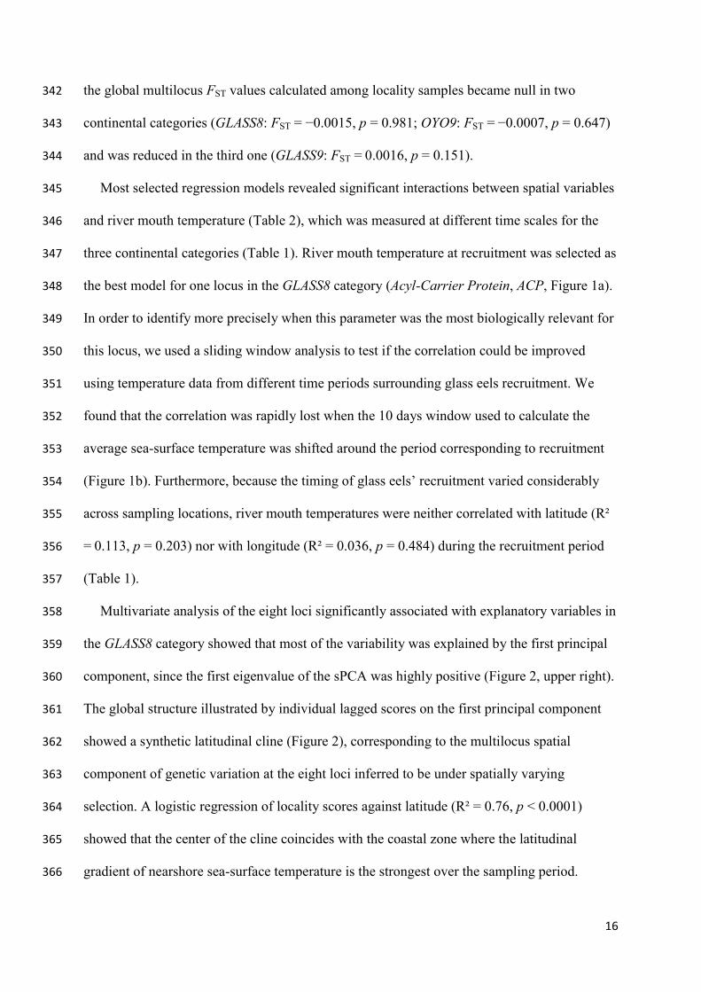
three continental categories (Table 1). River mouth temperature at recruitment was selected as 347

the best model for one locus in the GLASS8 category (Acyl­Carrier Protein, ACP, Figure 1a). 348

In order to identify more precisely when this parameter was the most biologically relevant for 349

this locus, we used a sliding window analysis to test if the correlation could be improved 350

using temperature data from different time periods surrounding glass eels recruitment. We 351

found that the correlation was rapidly lost when the 10 days window used to calculate the 352

average sea­surface temperature was shifted around the period corresponding to recruitment 353

(Figure 1b). Furthermore, because the timing of glass eels’ recruitment varied considerably 354

across sampling locations, river mouth temperatures were neither correlated with latitude (R² 355

= 0.113, p = 0.203) nor with longitude (R² = 0.036, p = 0.484) during the recruitment period 356

(Table 1). 357

Multivariate analysis of the eight loci significantly associated with explanatory variables in 358

the GLASS8 category showed that most of the variability was explained by the first principal 359

component, since the first eigenvalue of the sPCA was highly positive (Figure 2, upper right). 360

The global structure illustrated by individual lagged scores on the first principal component 361

showed a synthetic latitudinal cline (Figure 2), corresponding to the multilocus spatial 362

component of genetic variation at the eight loci inferred to be under spatially varying 363

selection. A logistic regression of locality scores against latitude (R² = 0.76, p < 0.0001) 364

showed that the center of the cline coincides with the coastal zone where the latitudinal 365

gradient of nearshore sea­surface temperature is the strongest over the sampling period. 366

17

Moreover, river mouth temperature averaged across the whole sampling period was a better 367

predictor of locality scores than latitude (R² = 0.88, p < 0.0001). A highly similar synthetic 368

latitudinal cline was obtained when analyzing the three continental categories together (see 369

Figure S3), supporting the temporal stability of the observed pattern. 370

One of the 13 SNPs associated with explanatory variables was a non­synonymous 371

polymorphism (Nucleolar Complex Protein 2, NCP­2), whereas for 9 of the 12 other SNPs, at 372

least one non­synonymous segregating site was identified within a 1kb region (see Figure S4). 373

Heterozygosity within the 13 contigs usually followed a monotonical trend and substantial 374

levels of linkage disequilibrium (r² > 0.5) were sometimes found between remote SNPs. 375

These results suggest that the indirect influence of selection through linkage with a nearby 376

functional mutation was more likely than direct selection at the focal SNPs. However, this 377

should not introduce any bias in the estimation of the relative fitness values used in the 378

following simulations. 379

380

Assessment of polymorphism stability under Levene’s model: 381

382

Simulating the evolution of allelic frequencies for the eight loci significantly associated 383

with explanatory variables in the GLASS8 category led to two different predictions. Under the 384

hypothesis of uniform contribution among niches and an effective population size (Ne) of 105, 385

simulations predicted polymorphism stability for two SNPs and allele fixation for the 386

remaining six loci (Table 3). The simulated evolution of allelic frequencies over generations 387

as generated by the model can be found for each of the eight loci Figure S5. Frequency at 388

equilibrium was fairly close to that measured in the SAR7 sample for the two SNPs predicted 389

to be protected by spatially varying selection. Concerning the six transient polymorphisms, 390

allele fixation was generally reached within less than 80 generations. Most importantly, the 391

18

invading allele was always the derived state after identifying the ancestral allele through 392

BLASTN search. 393

The results obtained under different assumptions on the relative contributions among 394

niches and population size did not radically change these predictions, as the same two 395

protected polymorphisms were repeatedly inferred across scenarios. However, estimating the 396

niche­specific relative fitness directly from the observed genotypes frequencies in the 397

GLASS8 category (i.e. instead of using values predicted by the regression models) increased 398

the number of protected polymorphisms from two to four (see Table S4). 399

400

DISCUSSION 401

402

Evidence for single­generation footprints of spatially varying selection: 403

404

Our results provide strong indications that young glass eels colonizing different areas of 405

the species range are exposed to differential patterns of selection, resulting in significant shifts 406

in allele frequencies within a short timescale. The alternative hypothesis of a subtle neutral 407

population genetic structure in the American eel was not supported by previous works, since 408

panmixia has never been rejected based on neutral markers (AVISE et al. 1986; WIRTH and 409

BERNATCHEZ 2003). This conclusion was reiterated here based on 60 neutral SNPs genotyped 410

over 944 individuals distributed across three temporal categories. Moreover, a neutral pattern 411

imposed by spatially restricted gene flow is not consistent with the finding that 85% (11 out 412

of 13) of the loci associated with explanatory variables were also detected as outliers, and that 413

different regression models were selected across these markers. Consequently, our data do not 414

support the existence of a spatial population structure due to deviation from panmixia in A. 415

rostrata. Alternatively, passive genotype­specific habitat choice could possibly occur if the 416

19

genes associated with environmental variables underlie differences in leptocephalus stage 417

duration. However, the observation that early­metamorphosing leptocephali preferentially 418

recruit to the center of the continental distribution range, whereas late­metamorphosing larvae 419

mostly settle in northern and southern locations (WANG and TZENG 1998) is inconsistent with 420

the clinal multilocus spatial component detected at these loci (Figure 2). Moreover, half of 421

these loci displayed HWE deviations in continental samples but not in the larval sample, 422

which is incompatible with the habitat choice hypothesis. Therefore, we propose that spatially 423

varying selection is the most parsimonious mechanism underlying the observed patterns of 424

genetic variation. 425

The diversity of the statistical models retained to explain genetic variation across selected 426

loci may suggest the implication of different locus­specific selective factors. Without detailed 427

information on such agents, the choice of spatial and temperature variables as proxies for the 428

ecological conditions experienced by eels was justified, as for instance several environmental 429

factors covary with latitude along the North Atlantic coasts (SCHMIDT et al. 2008). 430

Covariation between latitude and spatially varying selective factors has previously been used 431

to illustrate multilocus spatial patterns attributed to selection in heterogeneous environment in 432

Drosophila melanogaster (SEZGIN et al. 2004). Here, we additionally used this synthetic 433

multilocus signal to demonstrate the overall temporal stability of the observed patterns 434

(Figure S3). Owing to the apparent panmixia and the lack of evidence for large­scale habitat 435

choice in the American eel, any genetic pattern left by spatially varying selection at a given 436

generation will be inevitably erased at the next generation. Consequently, the temporal 437

stability of the observed genetic patterns between the GLASS8 and GLASS9 categories 438

probably reflects the repeated action of similar natural selection pressures in the two 439

consecutive year cohorts covered by this study. Given that only a very small proportion 440

(<0.5%) of the larvae survive until glass eels reach the coasts and that the glass eel survival 441

20

rate is about 10% (BONHOMMEAU et al. 2009), our sampling scheme was designed with the 442

intent to detect changes in allelic frequencies occurring during the early stages of eels’ life 443

cycle. Moreover, we sampled the first wave of early recruiting glass eels before potential 444

settlement cues may affect up­estuary migration depending on individual condition and 445

temperature (SULLIVAN et al. 2009). 446

Although we used variables that mirror continental factors better than open­ocean factors, 447

a decoupling between river mouth and nearshore continental shelf sea­surface temperatures in 448

the northeastern part of the species range (localities GAS, NF and PEI, Table 1) may have 449

influenced our results. Glass eels recruiting in this region during early summer first face cold 450

water temperatures while crossing the continental shelf before entering warmer estuary waters 451

influenced by river outflows. Differential mortality during the cross­shelf transport may thus 452

have resulted in the selection of explanatory models involving interactions between river 453

mouth temperature and latitude or longitude, as observed for six loci out of eight in the 454

GLASS8 category. This interpretation is further supported by the close correspondence 455

between the multilocus spatial variation component and the nearshore averaged sea­surface 456

temperature pattern in figure 2. Although it suggests that the continental shelf sea surface 457

temperature should have been used in the regression analyses, this variable remains too 458

difficult to measure without knowing the trajectories of eels during the cross­shelf transport. 459

Using hydrodynamic models for backtracking larval transport may thus help in selecting 460

additional meaningful variables in future studies. Admittedly, as in any other study of this 461

type, our approach cannot fully capture the signal of all spatially varying selection pressures, 462

and probably underestimates the number of genes under spatially varying selection. On the 463

other hand, the strong association found at locus Acyl­Carrier Protein (ACP) between allele 464

frequencies and temperature at recruitment (Figure 1) shows that the river mouth temperature 465

21

is a relevant variable. Indeed, settlement in estuaries is a critical period during which glass 466

eels do not feed (SULLIVAN et al. 2009) and probably live on their fatty acids reserves. 467

Three of the five allozymes previously studied (WILLIAMS et al. 1973) were included in 468

our analysis to assess whether clines observed at the protein level could be detected at the 469

DNA level. The SNP developed for the Malate dehydrogenase gene (MDH), which was also 470

detected as outlier in our initial 454 transcriptome scan, was the only one to show a significant 471

association with environmental variables. In the allozyme study, however, genetic 472

heterogeneity at this locus was only observed among samples of adults and not at the glass eel 473

stage. The lack of significant pattern for the SNPs developed at the ADH and PGI loci may be 474

due to problems of paralogy or to a lack of LD with the SNPs under selection. 475

476

The fate of selected polymorphisms under Levene’s model: 477

478

Covariation between environmental variables such as temperature and the direction and 479

strength of selection have been suspected for a long time to actively maintain polymorphisms 480

in heterogeneous environments (reviewed by HEDRICK et al. 1976; KARLIN 1977). Depending 481

on the overall sum of local selective effects, spatially varying selection can however lead to 482

two different outcomes: (i) balanced selection for different alleles in different environments 483

can maintain polymorphism’s stability over generations, while (ii) globally unbalanced local 484

effects of directional selection may lead to allelic fixation (LEVENE 1953). Recent theoretical 485

developments have shown that substantial multilocus polymorphism can be maintained under 486

Levene’s model, in particular when locally advantageous alleles are partially dominant 487

(BÜRGER 2010). This includes cases of local dominance that specifically arise with enzymes 488

when fitness is a concave function of the activity level while the heterozygote’s enzymatic 489

activity is intermediate to that of both homozygotes (GILLESPIE and LANGLEY 1974). 490

22

Here, equilibrium was tested through simulations under Levene’s model in order to 491

account for combinations of parameters leading to non­trivial evolution of allelic frequencies 492

within a finite population. This approach is relevant since the underlying conditions of 493

Levene’s model perfectly fit the American eel’s life cycle, which is characterized by random 494

mating and dispersal, and a local density regulation (VOLLESTAD and JONSSON 1988). While 495

exploring a realistic range of parameter values, stable equilibrium was predicted at only two 496

out of eight tested loci. This relatively low proportion may be partly explained by 497

uncertainties due to the methodological approach. For instance, a lack of precision in the 498

estimation of fitness parameters, but also in the relative outputs among niches, will obviously 499

affect the realism of the simulations (SCHMIDT and RAND 2001). Here, we only considered 16 500

river mouths among a much greater number of existing rivers harboring the American eel 501

along the North Atlantic coast. Yet, those sampling locations are distributed evenly across the 502

species range and are therefore representative of the variation in selection direction and 503

intensity potentially encountered by glass eels. By considering only the earliest life stages, we 504

may fail to catch differential selection acting later in the life cycle. While we cannot rule it 505

out, the fact that most of the mortality occurs before entering freshwater (BONHOMMEAU et al. 506

2009) reduces this possibility. Moreover, it is likely that selection acting at later life stages 507

plays on different sets of genes. Finally, successive waves of recruiting glass eels can face 508

different conditions depending on their date of arrival (i.e. sea­surface temperature), and inter­509

annual global variations in the selective parameters may also exist. The natural settings are 510

thus likely more complex than considered in the model. However, it has been showed that 511

temporal variation in selection is less efficient in maintaining locally adaptive polymorphisms 512

compared to spatially varying selection (EWING 1979). 513

Thus, it appears plausible that the low proportion of protected polymorphisms truly reflects 514

the relatively restrictive conditions required for equilibrium (LEVENE 1953). When a locally 515

23

advantageous allele appears by mutation and successfully escapes random loss when rare, it 516

has more chance to invade the panmictic gene pool and to become fixed than to stabilize at an 517

intermediate, stable frequency. Because the transitory phase to fixation will often last for a 518

few hundreds of generations, loci which are undergoing incomplete selective sweeps may not 519

be easily discovered unless they are frequent enough to be detected with a genome scan 520

approach. In populations with a large census size, however, new adaptive mutations can 521

frequently occur (KARASOV et al. 2010) and may result in selective sweeps if the overall 522

effects of spatially varying selection are unbalanced. The finding that, in our simulations, the 523

invading allele was always a derived state for each of the six predicted unstable SNPs 524

supports the hypothesis of linkage with such a globally advantageous mutation which has not 525

already reached fixation. 526

Incomplete sweeps are expected to leave a specific pattern in the haplotype structure. 527

Because the derived allele increasing in frequency has an atypically long­range LD compared 528

to neutral ancestral variants segregating at the same frequency (SABETI 2006; VOIGHT et al. 529

2006), the measure of LD can be used to detect ongoing directional selection. Here, sequence 530

information retrieved from 454 sequencing data was insufficient to perform such tests based 531

on the haplotype structure, which require phased haplotypes extending outside the selected 532

gene. However, measuring LD based on available information within contigs revealed the 533

existence of substantial linkage (r² > 0.5) between some sites which are likely separated by a 534

few kilobases if the presence of introns is taken into account. 535

536

Implications for adaptation and conservation of American eel: 537

538

The Gene Ontology (GO) molecular functions of the genes inferred to be involved in G×E 539

interactions mostly encompassed major metabolic functions, among which are found: lipid 540

24

metabolism (ANX­2: inhibition of phospholipase A2; ACP: acyl carrier activity; GPX­4: 541

phospholipid­hydroperoxide glutathione peroxidase activity), saccharide metabolism (MDH: 542

malate dehydrogenase activity; UGP­2: UDP­glucose pyrophosphorylase activity) and protein 543

biosynthesis (EIF­3F: translation initiation factor; PRP­40: Pre­mRNA­processing activity). 544

The best predictive models of all these genes included temperature, a factor known to have a 545

strong influence on the level of metabolism in the American eel (WALSH et al. 1983). 546

Moreover, the center of the synthetic multilocus latitudinal cline coincided with the region 547

where the warm waters of the Gulf Stream drift away from the coasts. Although the American 548

eel occupies a wide latitudinal range, its thermal preferendum is rather elevated for the 549

temperate zone, since glass eels have a highly reduced swimming ability below 7° 550

(WUENSCHEL and ABLE 2008), elvers optimally grow at 28° (TZENG et al. 1998), and yellow 551

eels stop feeding and become metabolically depressed below 10° (WALSH et al. 1983). 552

Therefore, selective effects are logically expected at the relatively low temperatures locally 553

encountered between metamorphosis and recruitment to estuaries, although phenotypic 554

plasticity may also account for the wide range of temperature tolerance in A. rostrata 555

(DAVERAT et al. 2006). 556

Two genes involved in defense response were also detected (CST: cysteine endopeptidase 557

inhibitor activity; SN4­TDR: nuclease activity). Since selective factors related to pathogen 558

exposure do not always correlate with temperature or geographic coordinates, other genes 559

whose variation patterns could not be explained with our set of explanatory variables may 560

also play a role in resistance to pathogens in A. rostrata. For instance, the innate immune 561

response gene TRIM­35 showed strong departure to HWE in glass eels and atypically high 562

levels of genetic differentiation between some localities (FST values up to 0.174). In parallel, 563

simulating the evolution of allelic frequencies at this locus based on observed genotype 564

frequencies predicted a stable equilibrium (result not shown). This observation warrants 565

25

further investigation, especially since the TRIM­35 gene cluster, which is located in a region 566

of significantly elevated nucleotide diversity in the threespine stickleback (Gasterosteus 567

aculeatus), is also a candidate target of balancing selection in this species (HOHENLOHE et al. 568

2010). 569

In conclusion, we have screened more than 13000 SNPs in transcribed regions of the 570

American eel genome and identified several genes undergoing spatially varying selection 571

associated with the highly heterogeneous habitat used by this species. Due to our 572

methodological approach, however, the number of genes involved in G×E interactions has 573

likely been underestimated, and the causative agents of selection remain partially unknown. 574

Nevertheless, the higher proportion of transient versus stable polymorphisms suggests that 575

locally adaptive polymorphisms are not easily maintained by spatially varying selection when 576

local adaptation is impossible. Under such conditions, theory predicts that phenotypic 577

plasticity, by broadening the environmental tolerance of individual genotypes, provides a 578

more functionally adaptive response to spatial environmental variation (SULTAN and SPENCER 579

2002). Indeed, the costs induced by selection on locally adaptive traits are particularly severe 580

in the case of random mating and in the absence of habitat choice (LENORMAND 2002). For 581

eels, as for other highly fecund marine species facing huge mortality rates during larval 582

stages, phenotypic plasticity may represent the main mechanism for coping with habitat 583

heterogeneity (EDELINE 2007), and our results suggest that differential expression of 584

paralogous genes may be involved in this regulation. Nevertheless, the finding of locally 585

selected mutations spreading to fixation in A. rostrata suggests that this high census size 586

species may be regularly subject to new locally adaptive mutations. How the recent 587

population decline of Atlantic eels (WIRTH and BERNATCHEZ 2003) affects their adaptability 588

to changing environments is still poorly understood and will be a matter of further 589

investigations. 590

26

591

Acknowledgments: We are grateful to M. Castonguay for his help in sample collection and 592

to R. MacGregor as well as anonymous referees and Associate Editor D. Begun for their 593

constructive and helpful comments on the manuscript. We also thank F. Pierron, M.H. 594

Perreault, V. Bourret and G. Côté for their precious help with molecular experiments and C. 595

Sauvage for help with bioinformatic analyses. This research was founded by a grant from 596

Natural Science and Engineering Research Council of Canada (NSERC, Discovery grant 597

program) as well as a Canadian Research Chair in Genomics and Conservation of Aquatic 598

Resources to L.B. P.A.G. was supported by a Government of Canada Post­Doctoral 599

Fellowship. M.M.H. was supported by the Danish Council for Independent Research | Natural 600

Sciences (grant 09­072120). 601

602

Author Contributions: L.B. and P.A.G. designed research; P.A.G. performed research; C.C., 603

M.H., E.N., P.A.G. contributed reagents/materials/analysis tools; P.A.G. Analyzed data; and 604

P.A.G., E.N., M.H. and L.B. wrote the paper. 605

606

607

27

FIGURES AND TABLES 608

609

Figure 1: Correlation between river mouth temperature and allele frequencies at locus ACP. 610

Logistic regression based on all 3 continental categories (a.). Allele frequencies in the 611

GLASS8 category are represented with black squares, OYO9 with light gray circles, and 612

GLASS9 with dark gray triangles. Sliding window analysis of the coefficient of determination 613

(R²) between allele frequencies at locus ACP in the GLASS8 category and the values predicted 614

based on river mouth temperature data (b.). For each day within a 3 month period centered on 615

the sampling date (which also corresponded approximately to the date of arrival at river 616

mouths), surface temperature was taken as the mean value across the 10 previous days. 617

618

619

620

621

28

Figure 2: Synthetic multilocus spatial variation component in the 2008 glass eels. The spatial 622

component analysis was based on genetic variation at the 8 loci significantly associated with 623

explanatory variables in the GLASS8 category. The 16 sampling sites are represented on the 624

map by squares colored according to each locality’s lagged score on the first principal 625

component, as indicated in the caption. Sea­surface temperatures averaged across the whole 626

sampling period (from Jan. 08th to Jul. 16th 2008) are represented on the same color scale for 627

indication (purple: 0.2°, red: 27.3°). The plot on the right shows the shape of the synthetic 628

multilocus cline, as well as the decomposition of the product of the variance and the spatial 629

autocorrelation into positive, null and negative components (upper right corner). The clinal 630

structure corresponds to the highly positive eigenvalue in red. 631

632

633

634

635

29

Table 1: Sampling location and date, sample size, developmental stage, and river mouth 636

temperature for each analyzed sample. 637

638

639

640

641

30

Table 2: Models selected for 13 loci associated with explanatory variables, for both the 642

GLASS8 dataset and the 3 continental categories. 643

644

645

646

Table 3: Simulated evolution of allelic frequencies under Levene’s model for the 8 loci 647

statistically associated with explanatory variables in the GLASS8 category. Uniform 648

contribution among niches and a population effective size of 105 were assumed in these 649

simulations. 650

651

652

653

31

LITERATURE CITED 654

655

ALTSCHUL, S. F., T. L. MADDEN, A. A. SCHAFFER, J. ZHANG, Z. ZHANG et al., 1997 Gapped BLAST and PSI‐656 BLAST: a new generation of protein database search programs. Nucleic Acids Research 25: 657 3389–3402. 658

ALTSHULER, D., V. POLLARA, C. COWLES, W. VAN ETTEN, J. BALDWIN et al., 2000 An SNP map of the human 659 genome generated by reduced representation shotgun sequencing. Nature 407: 513–516. 660

AVISE, J. C., G. S. HELFMANT, N. C. SAUNDERS and L. S. HALES, 1986 Mitochondrial DNA differentiation in 661 North Atlantic eels: Population genetic consequences of an unusual life history pattern. 662 Proceedings of the National Academy of Sciences 83: 4350‐4354. 663

BARRETT, J. C., B. FRY, J. MALLER and M. J. DALY, 2005 Haploview: analysis and visualization of LD and 664 haplotype maps. Bioinformatics 21: 263‐265. 665

BEAUMONT, M. A., and R. A. NICHOLS, 1996 Evaluating Loci for Use in the Genetic Analysis of Population 666 Structure. Proceedings of the Royal Society of London. Series B: Biological Sciences 263: 667 1619‐1626. 668

BONHOMMEAU, S., M. CASTONGUAY, E. RIVOT, R. SABATIÉ and O. LE PAPE, 2010 The duration of migration 669 of Atlantic Anguilla larvae. Fish and Fisheries 11: 289‐306. 670

BONHOMMEAU, S., O. LE PAPE, D. GASCUEL, B. BLANKE, A. M. TRÉGUIER et al., 2009 Estimates of the 671 mortality and the duration of the trans‐Atlantic migration of European eel Anguilla anguilla 672 leptocephali using a particle tracking model. Journal of Fish Biology 74: 1891‐1914. 673

BROCKMAN, W., P. ALVAREZ, S. YOUNG, M. GARBER, G. GIANNOUKOS et al., 2008 Quality scores and SNP 674 detection in sequencing‐by‐synthesis systems. Genome Research 18: 763−770. 675

BÜRGER, R., 2010 Evolution and polymorphism in the multilocus Levene model with no or weak 676 epistasis. Theoretical Population Biology 78: 123‐138. 677

CALCAGNO, V., and C. DE MAZANCOURT, 2010 glmulti: An R Package for easy automated model selection 678 with (Generalized) linear models. J Stat Soft 34: i12. 679

CHARLESWORTH, B., M. NORDBORG and D. CHARLESWORTH, 1997 The effects of local selection, balanced 680 polymorphism and background selection on equilibrium patterns of genetic diversity in 681 subdivided populations. Genetical Research 70: 155‐174. 682

DAVERAT, F., K. E. LIMBURG, I. THIBAULT, J. C. SHIAO, J. J. DODSON et al., 2006 Phenotypic plasticity of 683 habitat use by three temperate eel species Anguilla anguilla, A. japonica and A. rostrata. 684 Marine Ecology Progress Series 308: 231–241. 685

EDELINE, E., 2007 Adaptive phenotypic plasticity of eel diadromy. Marine Ecology Progress Series 341: 686 229‐232. 687

EWING, E. P., 1979 Genetic variation in heterogeneous environment VII. Temporal and spatial 688 heterogeneity in infinite populations. The American Naturalist 114: 197–212. 689

EXCOFFIER, L., and H. E. L. LISHER, 2010 Arlequin suite ver 3.5: a new series of programs to perform 690 population genetics analyses under Linux and Windows. Molecular Ecology Resources 10: 691 564–567. 692

FELSENSTEIN, J., 1976 The theoretical population genetics of variable selection and migration. annual 693 Review of Genetics 10: 253–280. 694

GARRIGAN, D., and P. W. HEDRICK, 2003 Perspective: detecting adaptive molecular evolution, lessons 695 from the MHC. Evolution 57: 1707–1722. 696

GILLESPIE, J. H., and C. H. LANGLEY, 1974 A general model to account for enzyme variation in natural 697 populations. Genetics 76: 837−884. 698

HANCOCK, A. M., D. B. WITONSKY, A. S. GORDON, G. ESHEL, J. K. PRITCHARD et al., 2008 Adaptations to 699 Climate in Candidate Genes for Common Metabolic Disorders. PLoS Genetics 4: e32. 700

HEDRICK, P. W., 1986 Genetic Polymorphism in Heterogeneous Environments: A Decade Later. Annual 701 Review of Ecology and Systematics 17: 535‐566. 702

32

HEDRICK, P. W., 2006 Genetic Polymorphism in Heterogeneous Environments: The Age of Genomics. 703 Annual Review of Ecology, Evolution, and Systematics 37: 67‐93. 704

HEDRICK, P. W., M. E. GINEVAN and E. P. EWING, 1976 Genetic Polymorphism in Heterogeneous 705 Environments. Annual Review of Ecology and Systematics 7: 1‐32. 706

HOEKSTRA, H. E., K. E. DRUMM and M. W. NACHMAN, 2004 Ecological genetics of adaptive color 707 polymorphism in pocket mice: geographic variation in selected and neutral genes. Evolution 708 58: 1329–1341. 709

HOHENLOHE, P. A., S. BASSHAM, P. D. ETTER, N. STIFFLER, E. A. JOHNSON et al., 2010 Population genomics of 710 parallel adaptation in Threespine stickleback using sequenced RAD tags. PLoS Genet 6: 711 e1000862. 712

JOMBART, T., 2008 adegenet: a R package for the multivariate analysis of genetic markers. 713 Bioinformatics 24: 1403−1405. 714

JOMBART, T., S. DEVILLARD, A. B. DUFOUR and D. PONTIER, 2008 Revealing cryptic spatial patterns in 715 genetic variability by a new multivariate method. Heredity 101: 92‐103. 716

KARASOV, T., S. W. MESSER and D. A. PETROV, 2010 Evidence that adaptation in Drosophila is not limited 717 by mutation at single sites. PLoS Genet 6: e1000924. 718

KARLIN, S., 1977 Gene frequency patterns in the levene subdivided population model. Theoretical 719 Population Biology 11: 356‐385. 720

KOEHN, R. K., and G. C. WILLIAMS, 1978 Genetic differentiation without isolation in the American Eel, 721 Anguilla rostrata. II. Temporal stability of geographic patterns. Evolution 32: 624−637. 722

KOLACZKOWSKI, B., A. D. KERN, A. K. HOLLOWAY and D. J. BEGUN, 2011 Genomic Differentiation Between 723 Temperate and Tropical Australian Populations of Drosophila melanogaster. Genetics 187: 724 245‐260. 725

KREITMAN, M., 1983 Nucleotide polymorphism at the alcohol dehydrogenase locus of Drosophila 726 melanogaster. Nature 304: 411–417. 727

LENORMAND, T., 2002 Gene flow and the limits to natural selection. Trends in Ecology & Evolution 17: 728 183‐189. 729

LEVENE, H., 1953 Genetic Equilibrium When More Than One Ecological Niche is Available. The 730 American Naturalist 87: 331‐333. 731

MAYNARD SMITH, J., 1966 Sympatric Speciation. The American Naturalist 100: 637‐650. 732 MCCLEAVE, J. D., and R. C. KLECKNER, 1982 Selective tidal stream transport in the estuarine migration of 733

glass eels of the American eel (Anguilla rostrata). Journal du Conseil 40: 262‐271. 734 MUNK, P., M. M. HANSEN, G. E. MAES, T. G. NIELSEN, M. CASTONGUAY et al., 2010 Oceanic fronts in the 735

Sargasso Sea control the early life and drift of Atlantic eels. Proceedings of the Royal Society 736 B: Biological Sciences 277: 3593‐3599. 737

NACHMAN, M. W., H. E. HOEKSTRA and S. L. D’AGOSTINO, 2003 The genetic basis of adaptive melanism in 738 pocket mice. Proceedings of the National Academy of Sciences 100: 5268–5273. 739

PELZ, H. J., R. S., M. HÜNERBERG, C. FREGIN, A. C. HEIBERG et al., 2005 The genetic basis of resistance to 740 anticoagulants in rodents. Genetics 170: 1839–1847. 741

PIERRON, F., E. NORMANDEAU, M. DEFO, P. CAMPBELL, L. BERNATCHEZ et al., 2011 Effects of chronic metal 742 exposure on wild fish populations revealed by high‐throughput cDNA sequencing. 743 Ecotoxicology 20: 1388‐1399. 744

PROUT, T., and O. SAVOLAINEN, 1996 Genotype‐by‐Environment Interaction is Not Sufficient to 745 Maintain Variation: Levene and the Leafhopper. The American Naturalist 148: 930–936. 746

PRZEWORSKI, M., 2002 The signature of positive selection at randomly chosen loci. Genetics 160: 747 1179–1189. 748

QUINLAN, A. R., D. A. STEWART, M. P. STRÖMBERG and G. T. MARTH, 2008 Pyrobayes: an improved base 749 caller for SNP discovery in pyrosequences. Nature Methods 5: 179–181. 750

SABETI, P. C., 2006 Positive Natural Selection in the Human Lineage. Science 312: 1614‐1620. 751 SCHMIDT, J., 1923 The breeding places of the eel. Philosophical Transactions of the Royal Society B: 752

Biological Sciences 211: 179−208. 753

33

SCHMIDT, P. S., and D. M. RAND, 2001 Adaptive maintenance of genetic polymorphism in an intertidal 754 barnacle: habitat‐and‐life‐stage specific survivorship of MPI genotypes. Evolution 55: 1336‐755 1344. 756

SCHMIDT, P. S., E. A. SERRAO, G. A. PEARSON and E. AL., 2008 Ecological genetics in the North Atlantic: 757 environmental gradients and adaptation at specific loci. Ecology 89: S91‐S107. 758

SEZGIN, E., D. D. DUVERNELL, L. M. MATZKIN, Y. DUAN, C.‐T. ZHU et al., 2004 Single‐Locus Latitudinal Clines 759 and Their Relationship to Temperate Adaptation in Metabolic Genes and Derived Alleles in 760 Drosophila melanogaster. Genetics 168: 923‐931. 761

STAPLEY, J., J. REGER, P. G. D. FEULNER, C. SMADJA, J. GALINDO et al., 2010 Adaptation genomics: the next 762 generation. Trends in Ecology and Evolution 25: 705‐712. 763

SULLIVAN, M. C., M. J. WUENSCHEL and K. W. ABLE, 2009 Inter and intra‐estuary variability in ingress, 764 condition and settlement of the American eel Anguilla rostrata: implications for estimating 765 and understanding recruitment. J Fish Biol 74: 1949‐1969. 766

SULTAN, S. E., and H. G. SPENCER, 2002 Metapopulation structure favors plasticity over local 767 adaptation. The American Naturalist 160: 271–283. 768

TESCH, F., 2003 The Eel. Blackwell Science Ltd., Oxford. 769 TURNER, T. L., E. C. BOURNE, E. J. VON WETTBERG, T. T. HU and S. V. NUZHDIN, 2010 Population 770

resequencing reveals local adaptation of Arabidopsis lyrata to serpentine soils. Nat Genet 42: 771 260‐263. 772

TZENG, W. N., Y. T. WANG and C. H. WANG, 1998 Optimal growth temperature of the American eel, 773 Anguilla rostrata (Le Sueur). J Fish Soc Taiwan 25: 111−115. 774

VOIGHT, B. F., S. KUDARAVALLI, X. WEN and J. K. PRITCHARD, 2006 A Map of Recent Positive Selection in 775 the Human Genome. PLoS Biology 4: e72. 776

VOLLESTAD, L. A., and B. JONSSON, 1988 A 13‐year study of the population dynamics and growth of the 777 European eel Anguilla anguilla in a Norwegian river: Evidence for density‐dependent 778 mortality, and development of a model for predicting yield. J Anim Ecol 57: 983−997. 779

WALSH, P. J., G. D. FOSTER and T. W. MOON, 1983 The effects of temperature on metabolism of the 780 American eel Anguilla rostrata (Le Sueur): compensation in the summer and torpor in the 781 winter. Physiol Zool 56: 532–540. 782

WANG, C.‐H., and W.‐N. TZENG, 1998 Interpretation of geographic variation in size of American eel 783 Anguilla rostrata elvers on the Atlantic coast of North America using their life history and 784 otolith ageing. Marine Ecology Progress Series 168: 35‐43. 785

WEILL, R., G. LUTFALLA, K. MOGENSEN, F. CHANDRE, A. BERTHOMIEU et al., 2003 Insecticide resistance in 786 mosquito vectors. Nature 423: 136–137. 787

WILLIAMS, G. C., R. K. KOEHN and J. B. MITTON, 1973 Genetic Differentiation Without Isolation in the 788 American Eel, Anguilla rostrata. Evolution 27: 192‐204. 789

WIRTH, T., and L. BERNATCHEZ, 2003 Decline of North Atlantic eels: a fatal synergy? Proceedings of the 790 Royal Society B: Biological Sciences 270: 681‐688. 791

WUENSCHEL, M., and K. ABLE, 2008 Swimming ability of eels (Anguilla rostrata, Conger oceanicus) at 792 estuarine ingress: contrasting patterns of cross‐shelf transport? Marine Biology 154: 775‐793 786. 794

YEAMAN, S., and S. P. OTTO, 2011 Establishment and Maintenance of Adaptive Genetic Divergence 795 under Migration, Selection, and Drift. Evolution 65: 2123‐2129. 796

797

798