1

The effect of reference point prices on mergers and acquisitions*

Malcolm Baker Harvard Business School and NBER

mbaker@hbs.edu

Xin Pan Harvard University

xinpan@fas.harvard.edu

Jeffrey Wurgler NYU Stern School of Business and NBER

jwurgler@stern.nyu.edu Abstract

Prior stock price peaks of targets affect several aspects of merger and acquisition activity. Offer prices are biased toward recent peak prices although they are economically unremarkable. An offer’s probability of acceptance jumps discontinuously when it exceeds a peak price. Conversely, bidder shareholders react more negatively as the offer price is influenced upward toward a peak. Merger waves occur when high returns on the market and likely targets make it easier for bidders to offer a peak price. Parties thus appear to use recent peaks as reference points or anchors to simplify the complex tasks of valuation and negotiation. JEL classification: G31; G34 Keywords: Mergers; Acquisitions; Offer Price; Reference Point; Behavioral Corporate Finance

*For helpful comments we thank an anonymous referee, the Honorable William Allen, Yakov Amihud,

Nick Barberis, Lauren Cohen, Ravi Dhar, Ming Dong, Robin Greenwood, Steven Huddart, Ulrike Malmendier, Florencia Marotta-Wurgler, Steven Mintz, Daniel Paravisini, Gordon Phillips, Gerald Rosenfeld of Rothschild North America, Rick Ruback, Meir Statman, Joshua White, Russ Winer, and seminar participants at Columbia University, Harvard Business School, Michigan State, the NBER Corporate Finance Summer Institute, NYU Stern, Queens University, the Rising Star Conference at RPI, and the Securities and Exchange Commission. Baker gratefully acknowledges financial support from the Division of Research of the Harvard Business School.

2

1. Introduction

The price that a bidding firm offers for a target is generally the outcome of a negotiation

with the target’s board. The standard textbook story emphasizes synergies. The offer price starts

with an estimate of the increased value of the combined entity under the new corporate structure,

deriving from cost reductions in labor or capital equipment, supply chain reliability, debt tax

shields, market power, market access and expertise, improved management, internal finance, and

other economic factors (e.g., Lang, Stulz, and Walkling, 1989 or Jovanovic and Rousseau, 2002).

This value gain is then divided between the two entities’ shareholders according to their relative

bargaining power. In theory, the textbooks suggest, all of this leads to an objective and specific

price for the target’s shares.

In practice, valuing a company is subjective. A large number of assumptions are needed

to justify any particular valuation of the combination.1 In addition, relative bargaining power

cannot be fully established. Boards can bluff in the negotiation. Other bidders could emerge.

These real-life considerations mean the appropriate target price cannot be set with precision, but

established only within a broad range. We hypothesize that this indeterminacy, in turn, creates

space for the price offered and its reception to reflect other influences, in particular the

psychological influences on the board of the target and the bidder and target shareholders, who

ultimately must approve the price.

In particular, we propose that salient but largely irrelevant reference point stock prices of

the target play roles in merger and acquisition activity through both the prices and the types and

quantities of firms traded. This psychological motivation has well-established roots in the

anchoring-and-conservative-adjustment estimation method (Tversky and Kahneman, 1974), the

salience of initial anchor positions in negotiations, and the prospect theory tenet that the utility of

an outcome is a function of the outcome’s distance from a reference point.

The reference point stock prices that we focus on are the peak prices that the target has

achieved over various horizons, such as the 13-week high, 26-week high, and so on. The 52-

week high price, for example, is routinely reported and discussed in the financial press and is

salient to executives, boards, and investors. Importantly, and in contrast to target shareholders’

individual cost bases, which represent other natural reference point prices for individuals, these

1Those who teach valuation analysis in business schools are painfully familiar with this fact.

3

peak prices are reference prices that are common across stakeholders. We start with some

anecdotes that suggest that practitioners do indeed give special weight to recent peak prices in

target valuations: Target firm boards that are discouraging the deal often point out that the bid is

below the recent high, while those that are encouraging the deal often note when the bid

compares favorably with that price.

We start by considering the relationship between recent peak prices and the offer price.

Our results show a visually and statistically obvious effect of recent peak prices. Histograms of

offer prices show spikes at the 13-week high, 26-week high, 39-week high, 52-week high, and

104-week high. In other words, a peak price often serves not merely as a subtle psychological

anchor but as one sufficiently heavy that there is no “adjustment” from it at all.

These peak prices are of incremental importance to the offer price decision. Controlling

for the 13-week high, the 26-week high price has a statistically and economically significant

effect on offer prices, and the 39-, 52-, and 65-week high prices also have independent

explanatory power. (The 65-week high price effect could arise because some deals take several

months to complete to the point that a formal public offer is announced, even if they begin with

the prevailing 52-week high as an anchor. Separate from that effect, it seems unlikely that the

private negotiation would in every case be so knife-edged, ignoring anything that fell, say, 53

weeks prior to announcement.) Having documented that multiple reference points matter, we

focus on the 52-week high for simplicity. For 52-week highs of a typical size, a 10% increase in

the 52-week high is associated with a 3.3% increase in the offer premium, controlling for a

variety of bidder, target, and deal characteristics.

The effect of peak prices on offer prices survives a variety of control variables,

robustness tests, and falsification tests. We examine the 52-week high’s effect on offer prices in

various subsamples and consider non-psychological alternative explanations. Most notably, the

52-week high could be proxying for the objective, but unobserved value gain from combination.

That is, it is the value to which the target assets could return if only they were managed as well

by the bidder in the future as they were by the target in the past. This agency- or information-

based hypothesis should perhaps be regarded as the null hypothesis. However, we find that the

52-week high of the market index also has a strong effect on offer prices. Because the market

component of the target’s 52-week high cannot be recovered merely by changing management,

this hypothesis cannot, at least not fully, explain the 52-week high effect on offer prices.

4

The second dimension of merger activity we consider is deal success—what distinguishes

bids that succeed from those that fail, and in particular whether the offer price’s relationship to

peak prices plays a role. Not surprisingly, higher offer prices are associated with higher

probabilities of deal success; we control for this effect with a fourth-order polynomial of offer

prices. The interesting finding is that an additional dummy variable indicates that the probability

of deal success increases discontinuously by 4.4% to 6.4% when the bidder makes an offer price

even slightly above the target’s 52-week high.

Bidder announcement effects have been extensively studied. One hypothesis is that they

include the market’s estimate of overpayment. The offer premium itself is not a clean measure of

overpayment, however, as better combinations may attract higher offer premiums. The 52-week

high is an ideal instrument for the effects of overpayment in mergers and acquisitions, separate

from synergies or misvaluation in the bidder. We find that the bidder’s announcement effect

becomes more negative with the target’s distance from its 52-week high. The bidder

announcement effect is 2.45% worse for each 10% increase in the component of offer premium

that is explained by the 52-week high; this is quite large relative to the unconditional bidder

announcement effects. Given the strong connection between 52-week highs and offer prices, an

interpretation is that shareholders of the bidder may view the bidder as more likely to be

overpaying when the target has fallen far below this reference price.

Apart from its impact on deal success and the value transfer in successful deals, high

peak prices may deter bidders from appearing in the first place. The fourth and last aspect of

merger activity that we examine is merger waves. It is well known that merger waves coincide

with higher recent returns and stock market valuations. The potential link to reference price

peaks is that higher market valuations mean that more targets are trading closer to their peak

prices. Therefore, these reference points may become easier to satisfy (from the perspective of

targets) and to justify (from the perspective of bidders) when valuations are high than when they

have fallen. In this section, we use time-series data and so our tests are less refined. Not

surprisingly, we find that the market’s 52-week high relative to its current value is inversely

related to the level of merger activity. More interesting is that the 52-week high matters

controlling for the past 12 individual monthly returns. The effects are somewhat stronger using

the 52-week high premium on firms that ex ante have typical characteristics of targets. A

5

comprehensive study of merger waves is beyond our scope; these results should be characterized

as preliminary evidence that the use of peak prices plays a role in merger waves.

To summarize, the use of reference point prices in mergers and acquisitions could shed

light on phenomena that standard theories do not fully explain. The most obvious is that they

help to explain offer premiums in a novel and economically significant fashion. The deal success

and market reaction implications of reference points are also somewhat unique. There are several

explanations for why merger volume and stock market valuations move together, however, such

as the market timing theories of mergers by Shleifer and Vishny (2003) and Rhodes-Kropf and

Viswanathan (2004); our results provide an additional explanation. Reference points do not shed

light on the nature of deal synergies (although nor do market timing or overconfidence theories).

Jovanovic and Rousseau’s (2002) Q-theory considers mergers as vehicles for technology transfer

and capital reallocation, addressing the market valuations-merger waves link and incorporating a

synergies story, and Jensen’s (1986) agency theory can explain synergies created by disciplinary

takeovers; neither theory has overlapping predictions with the dimensions of merger activity that

we study.2 The managerial theories of Amihud and Lev (1981) and Morck, Shleifer, and Vishny

(1990) or the overconfidence views of Roll (1986); Ben-David, Graham, and Harvey (2010); and

Malmendier and Tate (2008) are also distinct in their predictions. An interesting difference

between the reference point thinking and merger theories is that reference points embrace

considerations of the target, rather than focus on the bidder alone or features of the combination.

Of course, these are broad generalizations, and the literature on mergers and acquisitions is vast.

See Baker, Ruback, and Wurgler (2007) for a survey of behavioral theories of mergers (not

including a reference points perspective) and Andrade, Mitchell, and Stafford (2001) and

especially Betton, Eckbo, and Thorburn (2008) for surveys of the non-behavioral literature.

Section 2 proposes some hypotheses based on the anchoring and adjustment phenomenon

and briefly reviews related scientific and anecdotal evidence. Section 3 reviews the basic data.

Sections 4, 5, 6, and 7 report how reference points affect offer prices, deal success, offer

announcement effects, and merger waves, respectively. Section 8 summarizes and concludes.

2. The psychology of reference points, loss aversion, and anchoring and adjustment

2See also Maksimovic and Phillips (2001); Maksimovic, Phillips, and Prabhala (2011); Rajan, Volpin, and

Zingales (2000); and chapters in Kaplan (2000) on synergies and value enhancements.

6

The psychology of pricing is a recognized subfield of marketing research. There, the

focus is on identifying prices or “price points” that lead to discontinuous jumps in demand. The

merger and acquisition (M&A) context has several parallels. The bidder wants to offer the lowest

price that the target will accept: the target is the consumer to whom the bidder markets.

Unlike in retail pricing, of course, the target shareholders in a merger transaction are

selling not buying. The bidder is therefore looking for announced price points that will lead to

discontinuous jumps in supply. We briefly review some of the psychology and economics

relevant to the use of reference point prices.

2.1. Reference points, loss aversion, and anchoring and adjustment

The empirically-motivated prospect theory of Kahneman and Tversky (1979) identifies a

departure from preference specifications that emphasize levels of goods and wealth as the sole

drivers of value or utility. Their theory holds that changes in status relative to particular reference

points are also a carrier of perceived value. The reference point in their theory is derived from

the context at hand. It could be influenced by normatively-irrelevant frames of reference, or it

could be based on an aspirational level or expectation as opposed to the status quo (Kahneman,

1992).

Another component of preferences that Kahneman and Tversky (1979) emphasize is loss

aversion. This refers to a kink in prospect theory’s value function at its origin, specifically that

losses are disliked more than equal-size gains are liked. Furthermore, they set the shape of their

theory’s value function to include convexity in the domain of losses and concavity in gains to

help it explain finer features of observed choice. To summarize, their value function is shaped

like a kinked “S” and is defined over changes in value relative to a reference point.

The related phenomenon of anchoring and adjustment is associated with Tversky and

Kahneman (1974). It refers to a belief formation process (not a utility perception) under which

one begins at a specific initial value, salient but perhaps entirely irrelevant, and then adjusts

toward a final estimate based on other considerations. The bias typically observed is that the final

estimate is insufficiently adjusted from the initial value, hence its term “anchor.” The bias can

be used to an advantage in negotiations. Kahneman (1992) notes that “negotiators commonly

have an interest in misleading their counterpart about their reservation prices.… High claims and

7

low offers are therefore made in the hope of anchoring the other side’s view of one’s true

position… The moral of studies of anchoring is that such efforts at deception can succeed …

even when these messages are neither accepted nor even believed” (p. 309-310).

Economic applications of these ideas are plentiful. Neale and Bazerman (1991) consider

the setting of union negotiations over wages and review strategems that appear to take advantage

of the anchoring phenomenon. Babcock, Wang, and Loewenstein (1996) similarly report on the

self-serving use of comparison groups as reference points in wage bargaining. Camerer and

Malmendier (2007) consider reference point effects in organizational economics generally.

Northcraft and Neale (1987) show that the asking price affects estimates of the value of a house,

even among professional real estate agents who claim to view it as uninformative; but List (2003,

2004) and Plott and Zeiler (2005) qualifies this with evidence that experience attenuates or

eliminates the endowment effect.3 Genesove and Mayer (2001) find that homeowners’ cost

bases significantly affects negotiations and thus outcomes of real estate transactions. The large

literature on money illusion is based centrally on nominal reference point pricing.

The use of reference points among investors and other financial actors appears, for

example, in Shefrin and Statman (1985), who note that prospect theory and loss aversion imply

that investors have a “disposition effect” and are reluctant to sell stocks showing paper losses.

This effect is in Odean (1998); Grinblatt and Keloharju (2001); Grinblatt and Han (2005);

Ivković, Poterba, and Weisbenner (2005); and Birru (2011).4 Shefrin and Statman (1984) suggest

a view of dividends based on loss aversion and framing effects. Barberis, Huang, and Santos

(2001) discuss asset pricing implications of prospect theory, and Barberis and Xiong (2009)

emphasize that the 52-week high is a price in which investors are particularly willing to realize

gains. Degeorge, Patel, and Zeckhauser (1999) show that executives strain to exceed salient

earnings per share (EPS) thresholds. Baker and Xuan (2009) find that the price at which the CEO

joined the company is a reference point for raising new equity. Loughran and Ritter (2002)

propose that reference-point preferences and mental accounting help to explain initial public

offering (IPO) underpricing, a view tested by Ljungqvist and Wilhelm (2005). Hart and Moore

3In this connection, it is noteworthy that most executives and investors are not involved in merger

transactions with any frequency, although their bankers could be. 4In unreported tests we considered the trading volume-weighted average price (e.g., Grinblatt and Han,

2005) as another reference price that could be relevant to merger activity. However, perhaps because of the inherent noisiness of our measure, as well as the fact that it pertains exclusively to target shareholders rather than a wider range of stakeholders, we found weaker results than those for the 52-week high.

8

(2008) develop contracting theory based on parties’ use of anchoring and psychological

reference points.

Certain of these actions are efforts to cater to investors who notice reference points such

as EPS and 52-week highs—for example, Huddart, Lang, and Yetman (2009) find stock market

volume and price effects around this reference stock price, and Heath, Huddart, and Lang (1999)

find that employee exercise of stock options doubles when their company’s stock price exceeds

its 52-week high.

2.2. The target

In a sufficiently large merger or acquisition, the transaction must be approved by the

management and shareholders of the target as well as those of the bidder. We start by discussing

empirical hypotheses that derive from the psychology outlined above. The most obvious

application involves the disposition effect, or the reluctance to realize losses relative to a

reference point. While for some investors the reference point is likely to be their purchase price,

i.e., the disposition effect documented in papers mentioned above, other important reference

points—and, importantly for our purposes, ones that are common across shareholders—are the

firm’s recent peak prices. The 52-week high price, for example, is widely reported in the

financial media. Furthermore, because it by definition is a fairly recent price, it seems attainable

by target shareholders even in the absence of a merger. This logic predicts that targets are more

likely to approve mergers in which the offer price approaches or exceeds a recent peak price.

More subtly, the S-shaped value function predicts that the further is the current price from a

recent high, the less influence the marginal dollar away from that reference will have in terms of

the perception of losses.

Belief formation via anchoring and adjustment may reinforce the utility effects—and at

least three levels, two psychological and one practical. First, target shareholders must form an

estimate of target value when deciding whether to accept the offer. Lacking time, information,

and ability to accurately compute present values of future cash flows under alternative ownership

and management scenarios, some of them will consult recent peak prices as references. Second,

targets seek and attempt to justify the highest possible price. Whether or not the target board

views it as relevant, a recent peak price can be used as a negotiating anchor. The 52-week high

can be the highest salient and specific price at hand. Third, the target’s management and board

9

faces a risk of shareholder litigation if they recommend selling at a price that is viewed as too

low. That they did not sell below a recent peak price provides some rhetorical cover.

2.3. The bidder

The bidder’s psychology can also be affected by anchoring and adjustment both directly

and strategically. When pursuing a target, the bidder has to decide how much it is willing to pay,

and that in turn depends on how it values the target. It is not possible to pin this down with

certainty. An input to this estimation must be the target’s recent valuations, and as such its own

recent peak prices may enter as anchors. The bidder may reason, “if the target was valued at a

certain level just a few months ago, shouldn’t we, with our ability to realize synergies, value it

near or above that same level?” Thus a peak price can become an anchor, and as mentioned

above insufficient adjustment from that level becomes the norm.

Reinforcing predictions arise from the fact that bidder management must justify their

offer to shareholders and financiers. The management could reassure such stakeholders with the

simple argument that the target was worth that price in the past and so, of course, it must be

possible to realize that in the future. On the other hand, if the bidder’s investors do not think as

hard as its board about the target’s potential valuation, they can be less biased by the anchoring

phenomenon and so more likely to view peak-price-driven bids as overpaying.

And there is the bidder’s perception of the target’s psychology. Once a target valuation is

established by any means, the bidder must estimate the minimum price that the target will accept.

Boards may predict that the target’s 52-week high will be used both as a strategic anchor against

them in negotiations and as a reference point that their own investors care about.5 Or, bidders

may appreciate that targets want a “fair” offer and, knowing that targets have a biased notion of

fairness (Babcock, et al., 1995), offer a recent peak price even if they view it as too high.

2.4. Anecdotes from shareholder communications

The 52-week high price is often cited in communications between managements and

shareholders about pending mergers or acquisitions. It is also cited by the media as a simple

5In an interview with one of the authors, Gerald Rosenfeld, CEO of the investment bank Rothschild North

America, stated that in his experience the target’s current price is the most important reference for valuation while the 52-week high is the second-most critical reference.

10

yardstick with which to put the bid price in context. We mention a few anecdotal examples here;

the remainder of the paper provides a large sample analysis, but cannot provide as much color.

Commonplace are examples in which the offer price is generically compared to the 52-

week high. “Microsoft’s $31-per-share offer – $44.6 billion – represented a 62 percent

premium to Yahoo’s closing price late Thursday, although it’s below Yahoo’s 52-week

high of $34.08 reached less than four months ago” (Delaney, Guth, Karntschnig, 2008).

The article failed to explain why an historical price more than 78% higher than the

current price should be relevant to any party involved, however. But a subsequent article

was even more explicit. “Typically, boards of directors demand that a buyer pay at least

the company’s 52-week intraday high. That would be $34.08, 10% above Microsoft’s

$31-per-share offer and 16% above where it moved yesterday, to $29.33” (Karnitschnig

and Delaney, 2008). Note that the 52-week high was still retained as a critical benchmark

despite the considerable effect of the offer itself on the price.

The following article is noteworthy for featuring no less than four comparisons of targets

with their 52-week highs, including this deal—here, from the bidder’s perspective

regarding concerns about high prices: “Brocade Communications (BRCD) rose as an

M&A potential target in late summer and shares have held their own despite the thought

that many feel a merger here would have to come at too high of a premium for a buyer…

Shares were at $5.15 on our first go-round, now shares trade around $5.80. The 52-week

trading range is $4.64 to $9.45 and the market cap is roughly $2.6 billion”

(247wallst.com, October 26, 2010).

The 52-week high can of course also be cited as reason to embrace, not reject, an offer.

Fig. 1 shows an example slide from a shareholder presentation by Cablevision to its

shareholders on October 24, 2007. In arguing for acceptance of the offer from the family

which already controlled the company, Cablevision management highlights the fact that

the bid price is at a premium to a variety of 52-week high and low prices, an appeal both

to anchoring as an estimate of value and reference point utility.

11

Concerns about recent price peaks could also affect aggregate merger activity, which we

study in detail later in the paper. Douglas Braunstein, the head of investment banking at

JP Morgan Chase, stated: “… 50% of the companies in the S&P had share prices that

were within 10% of the 52-week low. Today, 50% of the companies in the index are

within 10% of the 52-week high. That means that sellers are more likely to think they

could get a fair value for their companies, while buyers aren’t going to shell out hefty

premiums to narrow the price gap” (Wall Street Journal, April 15, 2010). This example

also suggests the possibility that the market high price may determine offer premiums at

the firm level, another idea that we will explore.

An important takeaway from these anecdotes is that reference points may be salient to a

variety of agents involved in a merger transaction—advisors, boards, investors and financiers of

both the bidder and the target, and the media (which is important to the extent that it helps to

inform and shape the views of smaller investors). It is precisely because reference point prices

can affect so many stakeholders in a given transaction that we focus the empirical work on

documenting the effects of reference point prices on specific merger outcomes. In other words,

the odds of success in our empirical work increases from the numerous overlapping and

reinforcing predictions noted above. At the same time this makes it difficult to provide a full

attribution of our results to particular categories of agents, psychological mechanisms, and

negotiating strategies.

3. Data

3.1. Merger and acquisition sample

The sample of deals is described in Table 1. Our source for M&As is Thomson Financial.

We start with all unique deals (unique bids) in which the announcement date is between January

1, 1984, and December 31, 2007, where the target is a public company, in which the offer price

is not missing, and where the bidder starts with less than 50% of the target firm shares

outstanding and ends with 100% or else the percentage acquired is unknown. We exclude deals

that are missing an offer price or have been classified by Thomson as recapitalizations,

repurchases, rumors, or target solicitations. These constitute the minimal set of exclusions

12

required for our analysis. Of these deals, we were able to compute the target’s 52-week high

price from the Center for Research in Security Prices (CRSP) for a final sample of 7,020.

We define the offer premium as the total consideration offered scaled by the target’s price

as of 30 days prior to the announcement. Similarly, the 52-week target (market index) high is the

52-week high stock price (market index) over the 335 calendar days (two year window) ending

30 days prior to the announcement date expressed as a percentage difference from the CRSP

stock price (market index) 30 calendar days prior to the announcement date. The CRSP market

index is formed using total market value-weighted returns. The purpose of scaling these prices

by a common factor is to eliminate heteroskedasticity that would result from comparing them in

raw form. The purpose of choosing a 30-day lagged price as this scaling factor is to attenuate any

upward rumors or new information effect on the offer premium. See Schwert (1996) for the

relationship between offer premiums and pre-offer price runups.

For all deals, Thomson gives information on whether the offer is a tender offer and

whether the bidder is a financial buyer (LBO). For a subset of deals, we have information on the

form of payment is cash, stock, or other, whether the deal is completed or withdrawn, and

whether the bidder attitude is hostile, friendly, or neutral. We are able to determine the form of

payment for 6,309 deals and attitude for 7,020 deals, 263 of which were hostile. Of our main

sample, 1,199 are tender offers and 178 are acquisitions by financial buyers. It is likely that

Thomson is underreporting these deals, particularly the frequency of leveraged buyouts in recent

years. We keep track of the success of specific offers, not whether the target is ultimately

acquired. Like Betton and Eckbo (2000), we are concerned with all bids, from the first to the last.

Of the 6,462 deals that Thomson records as either completed or withdrawn, 25% are withdrawn.

Of course, this includes situations in which a competing or revised offer emerged, so the rate of

overall success is much higher than these averages would indicate.

3.2. Summary statistics

Table 2 reports means, standard deviations, medians, and extreme values for deal pricing,

outcome variables, and control variables. Regarding prices, the median offer premium is 29.19%,

the median 13-week high target price is 7.51%, etc. By definition, peak prices weakly increase

with horizon, reaching a median of 30.08% when looking at a two year window. The median 52-

week high market price is 2.64%. These are all expressed in log terms. For the peak prices,

13

which are positive by definition, we Winsorize at the 1% and 99% levels, but wide variation

remains.

In addition to the primary variables of interest, we record secondary deal outcome

variables in Panel B, and deal, target, and bidder characteristics in Panel C. All continuous

variables among these are also Winsorized. We calculate the three-day announcement return of

the bidder by compounding the daily holding period return from CRSP (CRSP: RET) centered

on the announcement date from Thomson. The median is -0.85%. About 75% of the offers are

successfully completed.

The target and bidder characteristics are from standard sources. The return on assets is

defined as net income (NI) divided by total assets (Compustat: AT). The book-to-market ratio is

defined as book equity divided by market equity, in which book equity is total shareholders’

equity (Compustat: SEQ) plus deferred taxes and investment tax credit (Compustat: TXDITC)

minus the redemption value of preferred stock (Compustat: PSRKRV), and market equity is

calculated by multiplying shares outstanding (CRSP: SHROUT) and price (CRSP: PRC) at fiscal

year end. The earnings price ratio is defined as earnings before interest and taxes (Compustat:

EBIT) divided by market equity (ME). Because not all target and bidder companies within the

main sample of 7,020 deals were tracked by Compustat in the year before the announcement of

the deal, we have financial ratios of the target for only 4,624 deals and of the bidder for only

1,900 deals.

The price volatility and monthly returns of the target (not shown) are from CRSP.

Volatility is defined as the standard deviation of daily returns for the 365 calendar days ending

30 days prior to the announcement date. Returns are calculated by compounding the daily

holding period return (CRSP: RET) for the appropriate period ending 30 days prior to the

announcement date. Market capitalization is price (CRSP: PRC) times shares outstanding

(CRSP: SHROUT) from CRSP at the fiscal year end prior to Thomson’s announcement date.

Panel C of Table 2 summarizes our battery of controls. Over the sample period, 44% of

the deals are financed with cash, 30% are financed with stock, 17% are tender offers, 4% are

hostile, and 3% are acquired by financial firms. As one would expect, targets are generally

financially weaker than bidders, including in valuation ratios with targets relatively more likely

to be value firms. One explanation is, of course, that poorly-managed firms become targets (e.g.,

Lang and Stulz, 1984 and Mitchell and Lehn, 1990).

14

4. Offer prices

4.1. Basic results

We begin by documenting the effect of past peak prices on offer prices, because this

relationship is central to the reference point perspective. Fig. 2 simply plots the density of offer

prices relative to the 13-, 26-, 39-, 52-, and 104-week highs. To keep the scale of the x-axis

manageable, we do not plot offer premiums that exceed 500% in absolute value.

The plots show clear spikes at the 13-week high, 26-week high, 39-week high, 52-week

high, and 104-week (two-year) high. The first price is weakly less than the second, which is

weakly less than the third, and so on, so we use regressions to verify the incremental importance

of peaks at each horizon. What the figures are able to prove on their own is that it is common to

offer exactly a recent peak price. To be clear, these peaks are not mechanically related to the

offer price setting its own peak price, because the most recent peak price we allow is 30 days

before the offer’s announcement. Whether a price is at or simply very close to the 52-week high

is not important economically.6 The takeaway from Fig. 2 is that peak prices play specific roles,

consistent with stories involving reference dependence.

Fig. 3 presents a formal discontinuity analysis of the 52-week high (for brevity we focus

on a single peak). Not only is the modal outcome equal to the 52-week high, but also now

another feature is revealed, which is that many other offers tend to collect just above the 52-week

high. This is most apparent when we divide offers into fewer bins in Panel B. This jump in the

distribution is statistically significant, with a p-value of 0.005 or less.7 Panel A shows yet

another interpretable feature. There is a slight decline in the density as we approach the 52-week

high from below, and a surge as we pass it. Some bidders could reason that if they were already

6Actually, in our later analysis of the probability of offer acceptance, we find that even tiny differences in

offer prices can affect economic outcomes. 7One concern is whether the discontinuity reflects discreteness in prices. Shares are quoted in sixteenths,

eighths, and decimals in our sample. The 52-week high is a price that has been observed in the price history of the target, so it falls on what might naturally be a mass point. A few refined show that this is not driving our discontinuity results. A discontinuity is apparent even when we drop the bin that contains the 52-week high. The p-value is 0.005 in Panel A and below 0.005 in Panel B. We have also estimated a bootstrap p-value by computing z-statistics for discontinuities around randomly chosen past target stock prices. Using this distribution, we find a p-value of 0.013.

15

considering a bid around this level, they may as well push it to just above the 52-week high to

increase the likelihood of acceptance—and this actually works, as we show later on.8

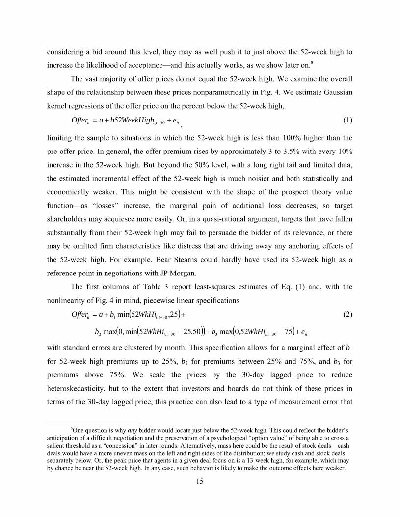
The vast majority of offer prices do not equal the 52-week high. We examine the overall

shape of the relationship between these prices nonparametrically in Fig. 4. We estimate Gaussian

kernel regressions of the offer price on the percent below the 52-week high,

ittiit eWeekHighbaOffer 30,52,

(1)

limiting the sample to situations in which the 52-week high is less than 100% higher than the

pre-offer price. In general, the offer premium rises by approximately 3 to 3.5% with every 10%

increase in the 52-week high. But beyond the 50% level, with a long right tail and limited data,

the estimated incremental effect of the 52-week high is much noisier and both statistically and

economically weaker. This might be consistent with the shape of the prospect theory value

function—as “losses” increase, the marginal pain of additional loss decreases, so target

shareholders may acquiesce more easily. Or, in a quasi-rational argument, targets that have fallen

substantially from their 52-week high may fail to persuade the bidder of its relevance, or there

may be omitted firm characteristics like distress that are driving away any anchoring effects of

the 52-week high. For example, Bear Stearns could hardly have used its 52-week high as a

reference point in negotiations with JP Morgan.

The first columns of Table 3 report least-squares estimates of Eq. (1) and, with the

nonlinearity of Fig. 4 in mind, piecewise linear specifications

25,52min 30,1 tiit WkHibaOffer (2)

ittiti eWkHibWkHib 7552,0max50,2552min,0max 30,330,2

with standard errors are clustered by month. This specification allows for a marginal effect of b1

for 52-week high premiums up to 25%, b2 for premiums between 25% and 75%, and b3 for

premiums above 75%. We scale the prices by the 30-day lagged price to reduce

heteroskedasticity, but to the extent that investors and boards do not think of these prices in

terms of the 30-day lagged price, this practice can also lead to a type of measurement error that

8One question is why any bidder would locate just below the 52-week high. This could reflect the bidder’s

anticipation of a difficult negotiation and the preservation of a psychological “option value” of being able to cross a salient threshold as a “concession” in later rounds. Alternatively, mass here could be the result of stock deals—cash deals would have a more uneven mass on the left and right sides of the distribution; we study cash and stock deals separately below. Or, the peak price that agents in a given deal focus on is a 13-week high, for example, which may by chance be near the 52-week high. In any case, such behavior is likely to make the outcome effects here weaker.

16

induces a spurious positive correlation. We therefore include the inverse of the 30-day lagged

price in all specifications.

The simple linear specification shows that offer prices rise about 1% for every 10% rise

in the 52-week high. This is statistically significant but not large. The true size of the effect is

masked by large outliers in the independent variable, which even when Winsorized includes

observations with values exceeding 250%. The piecewise linear specifications address this. They

show a magnitude similar to that suggested in Fig. 4, with a 10% higher 52-week high effecting a

roughly 3.3% higher offer price over the typical range of 52-week highs. As the 52-week high

reference price exceeds 25%, however, it exerts a smaller influence, rising at 1% for each

additional 10% increase in the 52-week high between 25% and 75%. Beyond 75%, the effect is

approximately 0.7%. This pattern is consistent with the S-shaped value function of prospect

theory, which implies that the further is the current price from the reference point, the less the

marginal perceived loss. However, there are other explanations.

The remaining columns test whether there is a specific interval over which peak prices

affect offer prices or whether peaks over several intervals have incremental explanatory ability.

We start with the 13-week high as a baseline regressor and add “incremental” high regressors at

13-week intervals until we reach back two years from the offer date. To estimate the incremental

26-week high regressor, for example, we essentially take the residual of a first-stage regression

of the 26-week high on the 13-week high. However, to allow for the incremental high to have a

diminishing marginal effect, we run this model three times to estimate the residual effects in

cases in which the 26-week high premium is below 25%, between 25% and 75%, and above

75%. The header to Table 3 details the empirical approach.

As Fig. 2 suggested, but could not show formally, there are incremental effects of peak

prices well beyond that achieved in the most recent 13 weeks. As an example, consider a

hypothetical Target A whose 13-week high (more precisely, the 9-week high ending 30 days

before announcement) is 10% higher than the period end price. Compare this target with another

Target B whose 13-week high premium is 0%. All else equal, the offer price for Target A will be

higher than the offer price for Target B by 4.6% to 4.7% on average. Subsequent peaks have

reasonably distinct effects on the offer price. Extending the example, suppose that Target A’s 26-

week high is 10% higher than one would expect, in a statistical sense, given its 13-week high and

Target B’s 26-week high is exactly what one would expect given its 13-week high. Then, the

17

offer price for Target A would be higher by a further 2.4% to 2.5%. There is also an incremental

peak at 65 weeks, which could reflect the fact that some mergers take months of negotiation, and

may anchor on the 52-week high at the beginning of the process. (It is also rather extreme to

assume that the private negotiation would be so knife-edged as to ignore anything beyond

precisely 52 weeks prior to announcement.) The effects of peaks beyond 65 weeks are generally

small and not statistically significant, with an anomaly being an incremental effect of the 78-

week high on offer premiums between 25% and 75%.

It is intuitive that long-past peaks are of progressively less relevance; the results here

suggest that there is a decline after 13 weeks and then a considerable drop after just over one

year. However, within the more recent period, a variety of peak prices matter. Having shown

this, we focus on the 52-week high for the rest of the paper. We stress that this is for simplicity.

There is plenty of analysis left to do just with one price. To repeat, there are incremental effects

at horizons within and slightly beyond 52 weeks, so the 52-week high appears not to be the

magic number here that it appears to be in some studies of volume and stock returns.

The peak price effect does not arise just because it reflects target firm returns over a pre-

specified period. Table 4 adds controls for each of the 12 months ending at t-30. This is another

effort to control for any effect of pre-offer runups on offer prices (Schwert, 1996). The peak

price effects are little changed. This indicates, in another way, that it is the return since the 52-

week high, i.e., the 52-week high premium, that drives the results, not that past returns were low

over some fixed interval.

The last specifications in Table 4 help to evaluate a possible non-psychological

alternative explanation. This explanation holds that the 52-week high price is particularly

relevant because it represents a specific valuation that the bidder could hope to obtain by

returning the target to “optimal” investment policy, in which optimal is defined as the policies

prevailing as of the time the high was reached, even in the absence of any synergies. This

explanation seems inconsistent with the evidence on the importance of incremental peaks shown

before. We evaluate this story further by replacing the target’s 52-week high premium with the

overall stock market’s 52-week high. The fact that this is also a statistically and similarly

economically significant predictor of offer prices casts more doubt on the alternative

explanation—the bidder cannot hope to recapture the market component of the target’s 52-week

high by returning it to a particular investment policy or correcting an agency problem.

18

Another, perhaps more complicated way of explaining this test is to think of the market

return as an instrument. An omitted variable in the regression of offer premiums on 52-week

high prices is firm specific mismanagement or potential synergy. The market 52-week high is

correlated with the nominal firm 52-week high, but is otherwise uncorrelated with firm specific

mismanagement. So, it satisfies the exclusion restriction. We chose not to present this as an

implied volatility (IV), because we were interested in the raw magnitude of the coefficient on the

market 52-week high.

While simple and brief, this test gives sharp evidence for the importance of specific

reference points. Like the spikes in Fig. 1, the results are not natural predictions of other theories

of offer premiums. We do not wish to dismiss these theories, of course. What we have shown is

that peak prices play an incremental role.9

If we take the sensitivity of the offer premium to the 52-week high as an arbitrary transfer

of value, we can compute the total value transfer for our sample. For each the 4,853 completed

deals in our sample, we multiply the 52-week high by the piecewise linear coefficients b in the

second column to estimate the component of the offer premium that is driven by the 52-week

high. To convert this quantity to dollars, we multiply it by the target market capitalization at t-30

to arrive at the transfer. The total value transfer is $116 billion, $24.0 million per deal, or 9.6%

of the total offer premium. Even under the assumption that the variation in the 52-week high is

entirely arbitrary, we cannot clearly identify whether this is overpayment or underpayment

without knowing the stand-alone fundamental value of the targets and the value of synergies

from the combinations. It is possible, for example, that on average the bidder gets a good deal,

but overpays when the target 52-week high is especially large relative to its current price. When

we discuss bidder announcement effects later, we will describe another estimate of the total

value transfer due to the target’s distance from its peak price, as well as an estimate of how that

distance affects the division of value created by the deal.

4.2. Robustness and other subsamples

9A specification that makes the similar points in a different way is to include the raw 52-week high and the market-adjusted 52-week high, which has a more rational flavor, to see which is more important in determining offer premiums. This is a little bit tricky to do with our piecewise linear specification, so we focus on the simple regression of the offer premium on the 52-week high, and we limit the sample to those situations in which the log of the 52-week high is less than 50%. We define the market adjusted return as the difference between the log of the firm 52-week high and the market 52-week high. The nominal 52-week high is driving our results; the market-adjusted high even has a slightly negative coefficient. These results are available upon request.

19

We report additional robustness and falsification tests in Table 5. We first examine the

influence of characteristics of the proposed transaction itself—whether it is for cash, stock,

hostile, a tender, or a financial bidder. Tender offers are associated with large increases in offer

prices, while financial buyers are associated with lower (but still substantial) offer premiums.10

These control variables do not diminish the effect of the 52-week high, nor do they increase the

total regression R2 as much as one might expect, presumably due to the relative scarcity of

tenders and financial buyers in our sample.11

We examine how the 52-week high effect compares with bidder and target firm

fundamentals as key inputs to offer premiums. We control for seven characteristics of the bidder

and the target. Large bidders bid more, while large targets receive less, as is intuitive when one

considers bids in dollar terms. A notable control for purposes of robustness is the target’s return

volatility. This is correlated with the 52-week premium and other peaks and could reflect aspects

of the target’s value to the bidder. Its significance as an incremental effect is not large; on the

other hand, the dummies for tender offers and financial buyers are strong in both economic and

statistical significance. While some of these controls are important determinants of offer prices,

their inclusion does not appear to greatly reduce the effect of peak prices.

The remaining columns conduct a falsification test. We look for a specific effect of the

52-week high in another way. We ask whether that price, as the 100th percentile price over the

past year, represents an effect distinct from the 90th percentile price, with which it is highly

correlated. The results show that despite this high correlation, the 52-week high effect comes

through. Furthermore, to the extent that the 90th percentile price also serves as an appropriate

proxy for fundamental valuation, this test, like that involving the market component of the 52-

week high, also casts doubt on the view that the 52-week high price effect reflects only that

channel. Results are similar for the 80th, the 95th, and even the 99th percentile of the target past

stock price distribution. Taken together, the figures and tables to this point provide convincing

evidence that offer prices are influenced by past peaks.

10See DeAngelo, DeAngelo, and Rice (1984) and Kaplan (1989) for early evidence on target shareholder

gains in LBOs, and Eckbo and Thorburn (2008) for a more recent survey of restructurings and LBOs. 11Heron and Lie (2006) examine the effect of 18 variables on offer premiums in a sample of 526 unsolicited

takeover bids. The character of their sample is different, but they also find that only a small number of factors significantly affect takeover premiums (largely related to the presence of poison pills and ownership structure). The most related result is that higher target returns over the prior year are associated with lower premiums. We control for lagged returns much more flexibly in Table 4, but note that their result is consistent with the negative coefficients we estimate for most lagged returns.

20

Results for a variety of subsamples are in Table 6. The first column shows that the effect

is stronger in tender offers. Because a tender offer is an appeal directly to target shareholders,

this reflects the perception of the bidder of the relevance of the reference point to target

shareholders, as opposed to the outcome of a negotiation with the target board or its advisors. A

related effect, perhaps, involves the attitude of target management. Hostile offers’ prices are a bit

more influenced by the 52-week high than friendly offers when the 52-week premium is

relatively high. One possibility is that hostile bidders consider this a lever to appeal directly to

target shareholders.

Reference points have similar effects on first offer and subsequent offers.12 The success

of the offer itself, while clearly endogenous as we show later (when we study the effect of the

offer price on the probability of success), provides an interesting sample split. Within the sample

of successful offers, bids more strictly adhere to the 52-week high price.

The form of payment is relevant to the reference point effect, although the interpretation

of the results is not unambiguous. The offer price in stock deals is more prone to reflect the 52-

week high when that price is relatively modest, while cash deals are more responsive to it when

it is higher, in other words when the target has recently fallen more sharply. One possibility is

that this reflects the communication and negotiation between bidders and their cash-providing

bankers. The bidders could be attempting to justify the offer price in part on the basis of the

target’s recent high.

The effect is strong in both halves of the sample, but generally somewhat lower in the

latter half. On the other hand, the effect has actually increased for medium-size 52-week high

premiums. Finally, in unreported results, we look at economic significance in another way. We

split the sample according to large (defined alternately as above the median cap of $100 million;

or above $500 million) and small targets. We find that the effect is at least as strong for deals

involving large targets. In light of the strong results both for recent years and within large firms,

the empirical effects seem to be of ongoing economic importance.

5. Deal success

12 Most offers in the sample are first offers, and indeed last offers also because most offers are successful. Be mindful that what we can observe are public first offers. Boone and Mulherin (2007) show that on the order of half of targets are sold in a competitive auction process that takes place prior to the first public offer; in other words, we often observe the outcome of that process.

21

Another important question is whether peak pricing affects deal success, leading to “real”

economic effects via capital reallocation. While evidence exists that investor psychology affects

numerous financial decisions such as corporate and mutual fund name changes, dividend policy,

nominal share pricing, and financing choices, strong evidence of behavioral phenomena having

real effects is not plentiful.13 A second feature of this analysis is that, like the tender offer

differential in the subsamples table, it focuses on the reception of the bid by the target’s

management, board, investors, and advisors. It thus could identify another aspect of merger

activity sensitive to anchoring and reference point utility considerations of those agents as

opposed to those of the bidder.

The precision of our prediction here makes for a straightforward test for such real effects,

and earlier anecdotes suggest that this is a plausible hypothesis. Suggestive of such an effect, the

probability of success across our sample is 69.9% if the offer price is below the 52-week high

and 78.3% if it is above.14 Table 7 tests for a discontinuity in a probit regression. Where S = 1 if

the deal is successful, we model

ittiitit eWkHiOffercbOfferaSpr 30,52

(3)

including control variables.15 One might expect that higher offer premiums are associated with

higher probabilities of success, as in e.g. Heron and Lie (2006). This specification allows us to

control for the level of the offer premium, unlike the cross-tab just reported, and thus to test

whether offer prices that are high relative to the 52-week high specifically enjoy an increased

probability of success. To ensure that c identifies a true discontinuity, we control for a quartic

polynomial of the offer price.

The results do indicate a discontinuous increase in the probability of target acceptance as

the offer price passes the 52-week high threshold. The effect remains identifiable upon the

13An exception is Polk and Sapienza (2009) who propose that catering to investor sentiment directly affects

corporate investment. 14Bear in mind that this is the success of a particular offer, not the overall rate of success in selling the

target to a given bidder. 15See Comment and Schwert (1995) and Heron and Lie (2006) for probit regressions of takeover attempt

success on a wider range of control variables, such as poison pills and pension overfunding. Their samples are much smaller and of a different character. In any case, given that only two out of 18 control variables in Heron and Lie’s models had p-values below 0.05, we felt that it was more important to preserve a reasonable sample size rather than require a large set of controls. It is also not clear what omitted factors would be correlated with the dummy variable of interest, as opposed to, perhaps, the polynomial terms of the offer price.

22

inclusion of additional control variables that contain explanatory power for deal success, such as

hostility (reducing success probability), tender (increasing), and bidder size (increasing). The

magnitude of the effect is a nontrivial 4.4 to 6.4 percentage point discontinuous increase in

success probability. The results are consistent with reference point behavior.16

Another implication of this logic is that when a bid comes in low relative to the 52-week

high, the bidder is more likely to revise it (perhaps under pressure from the target). The data on

revisions are very sparse, unfortunately, but we explored this implication in unreported tests. We

define a revision as an offer that follows a previous offer within 12 months. We code the revision

as +1 if the revision is upward, or zero if it is downward or if there is no revision.17 Then, we

repeat the analysis of success, but we replace success with the revision indicator as the dependent

variable. Interestingly, we found that when the offer premium is greater than the 52-week high,

the offer is 20% to 30% less likely to be revised, by our definition.

6. Bidders’ announcement returns

We next investigate how the bidder’s shareholders react to the news of the offer

premium, particularly the component of the offer premium that reflects the target’s 52-week

high. There are three distinct possibilities.

The first, and null hypothesis, is that the 52-week high has no impact on bidder returns.

That is, the effects we have discovered so far are about quantities, not the sharing of value

between the bidder and target. Under this explanation, the 52-week high dictates that a certain,

minimum premium be offered. Shareholders reject offers below this minimum but otherwise, the

52-week high has no impact on the split of value in successful bids. In this case, abnormal

returns would be unrelated to the peak price; any distortion would be in quantities not the

division of value.18 The second possibility is that the separation of ownership and control means

that the management of the bidder has reasons to pursue a combination that are independent of

shareholder value – or management and shareholders simply have different beliefs. In this case,

16More tentatively, taking the results at face value, they would suggest that the success of between 302 and

449 out of a total 7,020 offers could have been affected by whether the offer price fell above this threshold. 17When two bids arrive on the same day, we consider neither revised. This is a very broad definition of

revisions. Even with this broad definition, we only identify 80 target offers as subsequently revised. 18 We thank the referee for suggesting this hypothesis.

23

when an agency problem is combined with anchoring by target shareholders, targets with higher

anchor prices will be worse deals on average, and we will see a negative relationship between the

52-week high and bidder announcement returns. The third possibility is observationally

equivalent. It is the management of the bidder who is anchoring on past prices as well. In both

the second and third posisbilities, all of the distortion could be in the split of value, not in

quantities. In summary, the bidder announcement effect is useful in distinguishing whether the

market views the empirical relationship between the 52-week high and offer premia as relative

overpayment, or whether anchoring only restricts quantities.

To investigate these hypotheses we compute the 3-day cumulative market-adjusted return

at each bidder’s announcement and assess its sensitivity to the offer premium,

itittt ebOfferar 11 .

(4)

We start with ordinary least squares (OLS) but we are actually interested in the impact of the 52-

week high on the bidder returns as described above. We do this by examining IV slope estimates

in which the 52-week high is used as an instrument for the offer price. What we are doing with

an IV estimation is putting the 52-week in units of offer premia, so we can examine the chain of

responses from the 52-week high to the offer premium, and the offer premium to the bidder

return.

To be more specific, we use Eq. (2) as the first stage. To develop some more intution for

the IV estimates, imagine that the offer premium over the acquirer’s stand-alone value has two

components: synergies and overpayment. The bidder is either paying up for future cash flows

that cannot be realized by the target on its own or they are getting a good or a bad deal. If a large

offer premium is from synergies, the market should have a neutral reaction, or perhaps even a

positive one if the target is on average sharing the gains with the bidder. If a large offer premium

is from overpayment, then the market should have a negative reaction, because the bidder is

giving more up in consideration than it is receiving in future cash flow.

Now, consider the main result in the paper that the 52-week high is positively correlated

with the offer premium. In principle, this correlation could mean that the 52-week high is

positively correlated with either component. If the 52-week high effect reflects higher synergies,

then using it as an instrument in a regression of the market reaction on the offer premium will

lead to an IV estimate that is less negative or even positive when compared to the OLS estimate

that reflects both synergies and overpayment. If the 52-week high effect reflects overpayment,

24

then using it as an instrument should lead to an IV estimate that is more negative when compared

to the OLS estimate.

Table 8 shows the results of both approaches.19 Not surprisingly, the least-squares

estimates indicate that bidding shareholders react more negatively as the offer premium

increases. The magnitude of this effect is not overwhelming, as the third least-squares

specification indicates that a 10% increase in the offer premium is associated with a 0.40% (40

basis points) lower bidder announcement effect. One way to think about this small effect is that

particularly good combinations of bidders and targets could warrant a high offer premium. If so,

the market in general and bidder shareholders in particular recognize that a 10% higher offer

price does not mean 10% overpayment. Rather, the higher offer price reflects the omitted effect

of deal quality.

However, bidders’ shareholders are considerably more disappointed about the component

of the offer price that depends on a historical reference point. The last IV regression implies that

when the component of the offer premium driven by the 52-week high increases by 10%, the

bidder’s shareholders react with a considerable 2.45% lower announcement effect relative to the

average. This is large relative to the unconditional average announcement effect of -1.5%

(median of -0.85%) and it is several times larger than the comparable OLS estimate.20 Therefore,

if we use the market as a rough barometer, the 52-week high reflects over or underpayment not

synergies. The large difference between the OLS and IV results implies that bidder shareholders

consider 52-week-high-driven bids as overpaying – and that the first stage piecewise linear

specification makes an excellent instrument for pure overpayment, as opposed to simply higher

offers. Bidder shareholders are likely to suffer less from the anchoring or reference point utility

effects of past target prices, and more likely to view offers influenced by price peaks as a

manifestation of an agency problem.

If we take the sensitivity of the offer premium to the 52-week high as an arbitrary transfer

of value, we can take another look at the total value transfer for our sample. In the case of bidder

announcement returns, there is also the possibility of an incremental value loss. The bidder return

19Note that the sample in Table 8 is smaller than in previous analyses because we are limited by the

availability of the bidder’s announcement return (recall that our sample is not limited to publicly-traded bidders, only publicly-traded targets).

20Our results on unconditional announcement effects resemble those of Officer (2003). See Betton, et al. (2008) for a review of more than one dozen studies of bidder announcement returns—the range of results is surprisingly large.

25

can reflect the loss to its shareholders from overpayment for this deal and also a revaluation if

shareholders come to expect a bias toward overpayment in any future deals.

For each the 3,050 deals in our sample that are completed and in which the bidder is

publicly traded, we multiply the 52-week high by the piecewise linear coefficients b in the

second column of Table 3 to estimate the component of the offer premium that is driven by the

52-week high as before. We then multiply this effect on the offer premium by the coefficient b in

the third column of Table 8 to determine the bidder announcement return. To convert this to

dollars, we multiply this quantity by the bidder market capitalization at t-2 to arrive at the value

transferred or lost. The total is $430.0 billion, $140.9 million per deal, or 5.1 times the simple

value transfer. This suggests either a market overreaction or an incremental value loss stemming

from a realization that the bidder management has a tendency to overbid. Again, these economic

significance calculations include only the effect of the 52-week high price, not other peak prices.

However, obviously, they are subject to considerable error.

In observations in which the acquirer is also publicly traded, we can use the

announcement returns to estimate the total value created by the deal and also estimate the

division of that value between the bidder and the target. In particular, our previous results

suggest that targets that have fallen further will, all else equal, capture a bigger slice of the pie

than targets that are trading near their highs. Implementing this test must deal with the fact that

the change in market value of the bidder and target on announcement is negative 1,443 times in

our sample of 3,765 deals, involving a matched publicly traded target from CRSP. There can be

deals that have negative synergies, or these could be deals in which the announcement contains

other information about the bidder. This makes computing a simple division of value ratio

problematic.

Our approach, in results available upon request, is to fit the target announcement return

to the bidder announcement return, the log market capitalizations of the two firms, and

interaction terms. Positive residuals from this regression indicate deals in which the target has

captured a larger fraction of the value creation that would be predicted from the return of the

bidder and the overall size of the deal. We then replace the offer premium with this residual and

repeat the basic exercises in Table 3. Much like those basic results, we find that a 10% change in

the 52-week high in the first range of the piecewise linear regression (52-week high premiums up

to 25%) is associated with a 3.3% increase in excess value captured by the target.

26

7. Merger waves

We have documented that a given deal is more likely to go through if the bidder offers at

least the target’s 52-week high. But whether an offer appears in the first place depends on market

valuations. Bidders will all else equal find it easier to pay the 52-week high when it is at a

relatively small premium to current prices. A merger requires both an offer and its acceptance, so

a reference point channel can help to explain the coincidence of aggregate merger waves and

stock market valuations: 52-week high reference prices for targets will generally be more

affordable to bidders, relative to current prices, when the market has recently done well.

Those who are most knowledgeable about merger dynamics describe precisely this

mechanism. Recall an anecdote from earlier in the paper: In April 2010 the head of investment

banking at J.P. Morgan pointed out that many of the companies in the Standard and Poor (S&P)

“are within 10% of the 52-week high. That means sellers are more likely to believe they can get

a fair value for their companies, while buyers won’t have to shell out hefty premiums to narrow

the price gap” (Corkery, 2010).

To test for an effect of reference point prices on aggregate merger activity, we study

quarterly data on the number of mergers from Mergerstat Review from 1973 through 2007 and

examine its sensitivity to the 52-week market index high price,

ttt eWkHibaMergers 3052 . (5)

We normalize the raw number of mergers by the total number of firms on the NYSE and then

detrend by subtracting the average normalized level of quarterly merger activity over the trailing

2.5-year period starting before the 365 calendar days over which the market’s 52-week high is

calculated (thus, ten data points are involved in the detrending). The Mergerstat data include all

mergers involving public and private firms, so the annual total is often more than 100% of the

firms on the NYSE. The 52-week market index high price, now measured at quarterly frequency,

is again calculated from CRSP. Our analysis here is not meant to constitute a full investigation of

all aspects of merger waves, but rather to look for any evidence that might suggest a role for

peak prices. For detailed investigations of merger waves, see e.g. Harford (2005).

The first regression in Table 9 shows that the market 52-week high is a negative predictor

of quarterly merger activity, consistent with the most basic prediction. Specifically, when market

27

prices are ten percentage points below their 52-week high, the merger rate falls by 18% relative

to its trend. This fall represents 70% of the merger rate’s time-series standard deviation. Panel A

of Fig. 5 graphs this relationship. The inverse relationship is apparent.

We test some finer predictions. We calculate quarterly 52-week high series for high and

low book-to-market portfolios using monthly returns and value-sorted portfolios constructed by

Kenneth French. Shleifer and Vishny (2003) and Rhodes-Kropf and Viswanathan (2004) explain

acquisitions in terms of market timing, with richly-valued bidders pursuing lower-valued targets,

and Rhodes-Kropf, et al. (2005) and Dong, et al. (2006), among others, confirm that targets do

indeed have higher book-to-market ratios than bidders. Forming these portfolios thus allows us,

in a rough way, to separate firms that are relatively more likely to be targets from those more

likely to be bidders, which allows us to add a cross-sectional dimension to the analysis. For

simplicity, we refer below to low book-to-market firms as “bidders” and high book-to-market

firms as “targets,” while recognizing that the classifications are extremely coarse.

The next column shows that the decline in the merger rate associated with reference point

prices is even stronger when one calculates the reference price of targets alone. This is shown in

Panel B of Fig. 5. This result is unaffected by including the contemporaneous valuation level of

bidders, which is important for identifying an effect of the reference point theory incremental to

the market timing theory or any other explanation that predicts merger activity is positively

correlated with recent returns.

The remaining columns test further aspects of robustness. We include both the 52-week

high of bidding firms and the valuation level of target firms. Consistent with predictions, these

variables are unimportant in themselves and, more importantly, they do not alter inferences about

the importance of bidders’ reference prices. Finally, we control for lagged monthly returns,

which again have no effect on key inferences. This indicates that it is the specific drop from the

52-week high that matters, not the past return over any fixed past interval. Overall, the results

suggest that the reference point view helps to explain why merger waves arise and coincide with

stock market valuations and recent returns.

Finally, in results available upon request, we consider firm-level data in addressing

whether the pricing effects have an impact on the likelihood that an offer ever materializes. To

explore this, we merge our data on mergers and acquisitions in Table 1 back to the full CRSP

universe from 1984 through 2007. A shortcoming of this approach is that we could be missing

28

many merger offers, because of matching issues from Thomson to CRSP and because the

Thomson data is incomplete. (This is why the time-series analysis above may be preferable, in

addition to addressing merger waves per se.)

We regress the probability of a merger in each firm-month on the firm-specific 52-week

high price, expressed as a percentage of the price at the previous month end. We also

“instrument” with the market 52-week high. In effect we repeat the regressions in the first two

columns of Table 3 and the third column of Table 4, but with an indicator variable for a merger

offer as the dependent variable instead of the offer price and the entire CRSP universe rather than

just those firms targeted with an offer. For the market return and the range between zero and

25% of the 52-week high, the results are consistent with the pricing effects and intuitive

predictions. In other words, as a firm approaches its 52-week high from below, the chances of a

merger offer increase. The economic effects that we measure with this approach might seem

small, but this is because the unconditional probability of a merger offer is only 77 basis points

per firm-month. (This assumes that our merge with Thomson misses no offers.) In particular,

moving from a firm that is trading at a new high price to a firm that is trading 25% off of its high

price, the probability of a merger drops from 88 basis points to 77 basis points.

Above this level, the marginal effect of the 52-week high on the probability of a merger

increases, which contrasts with the pricing effects we observed in Table 3. However, those

pricing effects were also weaker, and intuitively, high prices should have less power as reference

points the further they are from current prices. Also, well over half the sample is trading within

25% of its 52-week high price. Matching Table 4, a 10% increase in the market 52-week high is

associated with roughly a five basis point reduction in the probability of a merger (again relative

to the unconditional average of 77 basis points).

8. Conclusions

We study the effect of the target’s past peak prices on various aspects of merger and

acquisition activity. We find that recent peak prices help to explain the bidder’s offer price;

bidder announcement effects; deal success; and, more speculatively, merger waves. From an

allocational perspective, the effect on deal success is particularly interesting, in that it constitutes

a real effect through the distribution of capital across investment opportunities.

29

The results of various falsification tests and robustness tests suggest that these effects are

not, as a group, easily reconciled with standard theories of mergers. Rather, we believe that the

most natural explanation is that reference point prices play a role in mergers-related decisions,

similar to their previously-documented roles in the contexts of real estate pricing, institutional

and individual stock trading, IPO underpricing, option exercises, and other settings.

30

References Amihud, Y., Lev, B., 1981. Risk reduction as a managerial motive for conglomerate mergers. Bell Journal of Economics 12, 605–617. Andrade, G., Mitchell, M., Stafford, E., 2001. New evidence and perspectives on mergers. Journal of Economic Perspectives 15, 103–120. Babcock, L., Wang, X., Loewenstein, G., 1996. Choosing the wrong pond: Social comparisons in negotiations that reflect a self-serving bias. Quarterly Journal of Economics 111, 1–19. Babcock, L., Loewenstein, G., Issacharoff, S., Camerer, C., 1995. Biased judgments of fairness in bargaining. The American Economic Review 85, 1337–1343. Baker, M., Ruback, R., Wurgler, J., 2007. Behavioral corporate finance: A survey. In: Eckbo, B. E. (Ed.), The Handbook of Corporate Finance: Empirical Corporate Finance vol. 1, New York. Baker, M., Xuan, Y., 2009. Under new management: Equity issues and the attribution of past returns. Unpublished working paper. Harvard Business School, Boston. Barberis, N., Huang, M., Santos, T., 2001. Prospect theory and asset prices. Quarterly Journal of Economics 116, 1–53. Barberis, N., Xiong, W., 2009. What drives the disposition effect? An analysis of a long-standing preference-based explanation. Journal of Finance 64, 751–784. Ben-David, I., Graham, J. R., Harvey, C. R., 2010. Managerial miscalibration. Unpublished working paper. Duke University, Durham. Betton, S., Eckbo, B. E., 2000. Toeholds, bid jumps, and expected payoffs in takeovers. Review of Financial Studies 13, 841–882. Betton, S., Eckbo, B. E., Thorburn, K., 2008. Corporate takeovers. In: Eckbo, B. E. (Ed.), The Handbook of Corporate Finance: Empirical Corporate Finance vol. 2, New York. Birru, J., 2011. Confusion of confusions: A test of the disposition effect and momentum. Unpublished working paper. New York University, New York. Boone, A. L., Mulherin, J. H., 2007. How are firms sold? The Journal of Finance 62, 847–875. Camerer, C. F., Malmendier, U., 2007. Behavioral economics of organizations. In: Diamond, P., Vartiainen H. (Eds.), Behavioral Economics and Its Applications, New Jersey. Comment, R., Schwert, G. W., 1995. Poison or placebo? Evidence on the deterrence and wealth effects of modern antitakeover measures. Journal of Financial Economics 39, 3–43. Corkery, M., 2010. Optimism? Yes. M&A? Not yet. Wall Street Journal, April 16, C3.

31

DeAngelo, H., DeAngelo, L., Rice, E. M., 1984. Going private: The effects of a change in corporate ownership structure. Midland Corporate Finance Journal summer, 35–43. Degeorge, F., Patel, J., Zeckhauser, R., 1999. Earnings management to exceed thresholds. Journal of Business 72, 1–33. Delaney, K. J., Guth, R. A., Karnitschnig, M., 2008. Microsoft makes grab for Yahoo --- Software giant’s bid is aimed at Google; tapping ads, customers. The Wall Street Journal, February 2, A1. Dong, M., Hirshleifer, D., Richardson, S., Teoh, S. H., 2006. Does investor misvaluation drive the takeover market? The Journal of Finance 61, 725–762. Eckbo, B. E., Thorburn, K., 2008. Corporate restructuring: Breakups and LBOs. In: Eckbo, B. E. (Ed.), The Handbook of Corporate Finance: Empirical Corporate Finance vol. 2, New York. Genesove, D., Mayer, C., 2001. Loss aversion and seller behavior: Evidence from the housing market. The Quarterly Journal of Economics 116, 1233–1260. Grinblatt, M., Han, B., 2005. Prospect theory, mental accounting, and momentum. Journal of Financial Economics 78, 311–339. Grinblatt, M., Keloharju, M., 2001. What makes investors trade? The Journal of Finance 56, 589–616. Harford, J., 2005. What drives merger waves? Journal of Financial Economics 77, 529–560. Hart, O., Moore, J., 2008. Contracts as reference points. Quarterly Journal of Economics 123, 1–48. Heath, C., Huddart, S., Lang, M., 1999. Psychological factors and stock option exercise. The Quarterly Journal of Economics 114, 601–627. Heron, R. A., Lie, E., 2006. On the use of poison pills and defensive payouts by takeover targets. The Journal of Business 79, 1783–1807. Huddart, S., Lang, M., Yetman, M. H., 2009. Volume and price patterns around a stock’s 52-week highs and lows: Theory and evidence. Management Science 55, 16–31. Ivković, Z., Poterba, J., Weisbenner, S., 2005. Tax-motivated trading by individual investors. The American Economic Review 95, 1605–1630. Jensen, M. C., 1986. Agency costs of free cash flow, corporate finance and takeovers. The American Economic Review 76, 323–329.

32

Jovanovic, B., Rousseau, P. L., 2002. The Q-theory of mergers. The American Economic Review 92, 198–204. Kahneman, D., 1992. Reference points, anchors, norms, and mixed feelings. Organizational Behavior and Human Decision Processes 51, 296–312. Kahneman, D., Tversky, A., 1979. Prospect theory: An analysis of decision under risk. Econometrica 47, 263–292. Kaplan, S. N., 1989. Management buyouts: Evidence of taxes as a source of value. The Journal of Finance 44, 611–632. Kaplan, S. N. (Ed.), 2000, Mergers and productivity. In: National Bureau of Economic Research Conference Report. The University of Chicago Press, Chicago. Karnitschnig, M., Delaney, K. J., 2008. Searching Yahoo for value. The Wall Street Journal, February 5, C1. Lang, L. H. P., Stulz, R. S., 1994. Tobin’s q, corporate diversification, and firm performance. Journal of Political Economy 102, 1248–1280. Lang, L. H. P., Stulz, R. S., Walkling, R. A., 1989. Managerial performance, Tobin’s Q, and the gains from successful tender offers. Journal of Financial Economics 24, 137–154. List, J. A., 2004. Neoclassical theory versus prospect theory: Evidence from the marketplace. Econometrica 72, 615–625. List, J. A., 2003. Does market experience eliminate market anomalies? The Quarterly Journal of Economics 118, 41–71. Ljungqvist, A., Wilhelm, Jr., W. J., 2005. Does prospect theory explain IPO market behavior? The Journal of Finance 60, 1759–1790. Loughran, T., Ritter, J. R., 2002. Why don’t issuers get upset about leaving money on the table in IPOs? Review of Financial Studies 15, 413–444. Maksimovic, V., Phillips, G., 2001. The market for corporate assets: Who engages in mergers and asset sales and are there efficiency gains? The Journal of Finance 56, 2019–2065. Maksimovic, V., Phillips, G., Prabhala, N. R., 2011. Post-merger restructuring and the boundaries of the firm. Journal of Financial Economics 102, 317–343. Malmendier, U., Tate, G., 2008. Who makes acquisitions? CEO overconfidence and the market’s reaction. Journal of Financial Economics 89, 20–43. Mitchell, M. L., Lehn, K., 1990. Do bad bidders become good targets?” Journal of Political Economy 98, 372–398.

33

Morck, R., Shleifer, A., Vishny, R. W., 1990. Do managerial objectives drive bad acquisitions? The Journal of Finance 45, 31–48. Neale, M. A., Bazerman, M. H., 1991. Cognition and rationality in negotiation. The Free Press, New York. Northcraft, G. B., Neale, M. A., 1987. Experts, amateurs, and real estate: An anchoring-and-adjustment perspective on property pricing decisions. Organizational Behavior and Human Decision Processes 39, 84–97. Odean, T., 1998. Are investors reluctant to realize their losses? The Journal of Finance 53, 1775–1798. Officer, M. S., 2003. Termination fees in mergers and acquisitions. Journal of Financial Economics 69, 431–467. Plott, C. R., Zeiler, K., 2005. The willingness to pay–willingness to accept gap, the “endowment effect,” subject misconceptions, and experimental procedures for eliciting valuations. American Economic Review 95, 530–545. Polk, C., Sapienza, P., 2009. The stock market and corporate investment: A test of catering theory. Review of Financial Studies 22, 187–217. Rajan, R., Volpin, P., Zingales, L., 2000. The eclipse of the U.S. tire industry. In: Kaplan, S. N. (Ed.), Mergers and productivity. University of Chicago Press, Chicago. Rhodes-Kropf, M., Viswanathan, S., 2004. Market valuation and merger waves. The Journal of Finance 59, 2685–2718. Rhodes-Kropf, M., Robinson, D. T., Viswanathan, S., 2005. Valuation waves and merger activity: The empirical evidence. Journal of Financial Economics 77, 561–603. Roll, R., 1986. The hubris hypothesis of corporate takeovers. The Journal of Business 59, 197–216. Schwert, G. W., 1996. Markup pricing in mergers and acquisitions. Journal of Financial Economics 41, 153–192. Shefrin, H. M., Statman, M., 1984. Explaining investor preference for cash dividends. Journal of Financial Economics 13, 253–282. Shefrin, H. M., Statman, M., 1985. The disposition to sell winners too early and ride losers too long: Theory and evidence. The Journal of Finance 40, 777–790. Shleifer, A., Vishny, R. W., 2003. Stock market driven acquisitions. Journal of Financial Economics 70, 295–311.

34

Tversky, A., Kahneman, D., 1974. Judgment under uncertainty: Heuristics and biases. Science 185, 1124–1131.

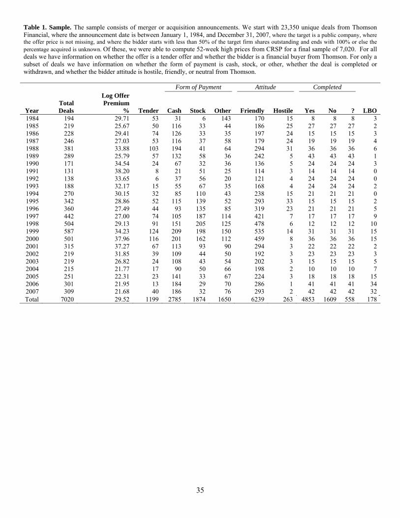
35

Table 1. Sample. The sample consists of merger or acquisition announcements. We start with 23,350 unique deals from Thomson Financial, where the announcement date is between January 1, 1984, and December 31, 2007, where the target is a public company, where the offer price is not missing, and where the bidder starts with less than 50% of the target firm shares outstanding and ends with 100% or else the percentage acquired is unknown. Of these, we were able to compute 52-week high prices from CRSP for a final sample of 7,020. For all deals we have information on whether the offer is a tender offer and whether the bidder is a financial buyer from Thomson. For only a subset of deals we have information on whether the form of payment is cash, stock, or other, whether the deal is completed or withdrawn, and whether the bidder attitude is hostile, friendly, or neutral from Thomson.

Form of Payment Attitude Completed

Year Total Deals

Log Offer Premium

% Tender Cash Stock Other Friendly Hostile Yes No ? LBO 1984 194 29.71 53 31 6 143 170 15 8 8 8 3 1985 219 25.67 50 116 33 44 186 25 27 27 27 2 1986 228 29.41 74 126 33 35 197 24 15 15 15 3 1987 246 27.03 53 116 37 58 179 24 19 19 19 4 1988 381 33.88 103 194 41 64 294 31 36 36 36 6 1989 289 25.79 57 132 58 36 242 5 43 43 43 1 1990 171 34.54 24 67 32 36 136 5 24 24 24 3 1991 131 38.20 8 21 51 25 114 3 14 14 14 0 1992 138 33.65 6 37 56 20 121 4 24 24 24 0 1993 188 32.17 15 55 67 35 168 4 24 24 24 2 1994 270 30.15 32 85 110 43 238 15 21 21 21 0 1995 342 28.86 52 115 139 52 293 33 15 15 15 2 1996 360 27.49 44 93 135 85 319 23 21 21 21 5 1997 442 27.00 74 105 187 114 421 7 17 17 17 9 1998 504 29.13 91 151 205 125 478 6 12 12 12 10 1999 587 34.23 124 209 198 150 535 14 31 31 31 15 2000 501 37.96 116 201 162 112 459 8 36 36 36 15 2001 315 37.27 67 113 93 90 294 3 22 22 22 2 2002 219 31.85 39 109 44 50 192 3 23 23 23 3 2003 219 26.82 24 108 43 54 202 3 15 15 15 5 2004 215 21.77 17 90 50 66 198 2 10 10 10 7 2005 251 22.31 23 141 33 67 224 3 18 18 18 15 2006 301 21.95 13 184 29 70 286 1 41 41 41 34 2007 309 21.68 40 186 32 76 293 2 42 42 42 32 Total 7020 29.52 1199 2785 1874 1650 6239 263 4853 1609 558 178

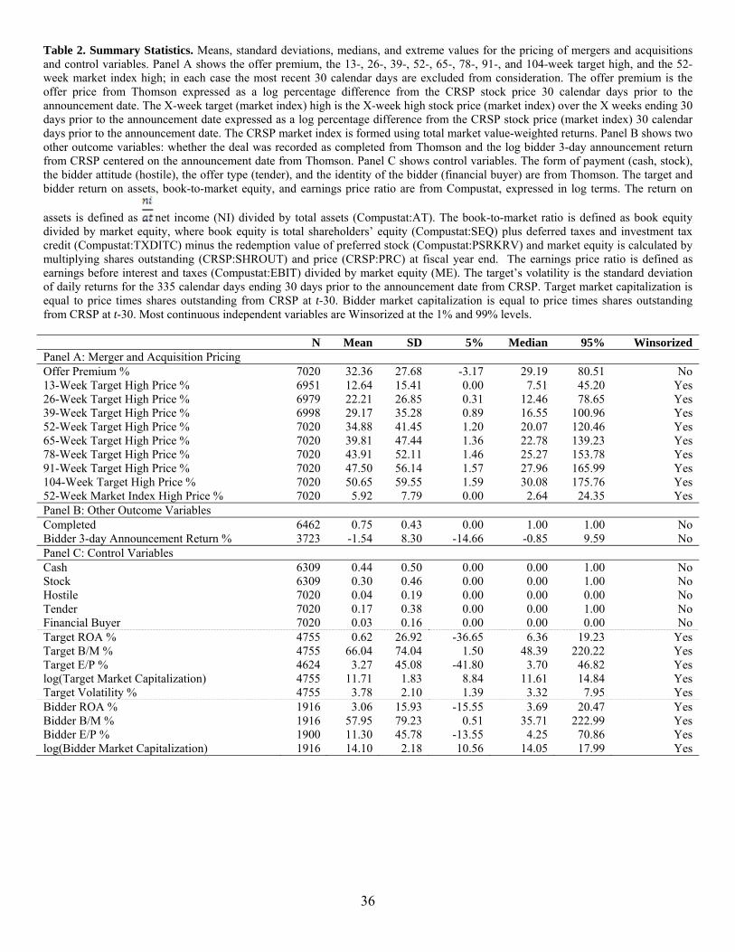
36

Table 2. Summary Statistics. Means, standard deviations, medians, and extreme values for the pricing of mergers and acquisitions and control variables. Panel A shows the offer premium, the 13-, 26-, 39-, 52-, 65-, 78-, 91-, and 104-week target high, and the 52-week market index high; in each case the most recent 30 calendar days are excluded from consideration. The offer premium is the offer price from Thomson expressed as a log percentage difference from the CRSP stock price 30 calendar days prior to the announcement date. The X-week target (market index) high is the X-week high stock price (market index) over the X weeks ending 30 days prior to the announcement date expressed as a log percentage difference from the CRSP stock price (market index) 30 calendar days prior to the announcement date. The CRSP market index is formed using total market value-weighted returns. Panel B shows two other outcome variables: whether the deal was recorded as completed from Thomson and the log bidder 3-day announcement return from CRSP centered on the announcement date from Thomson. Panel C shows control variables. The form of payment (cash, stock), the bidder attitude (hostile), the offer type (tender), and the identity of the bidder (financial buyer) are from Thomson. The target and bidder return on assets, book-to-market equity, and earnings price ratio are from Compustat, expressed in log terms. The return on

assets is defined as net income (NI) divided by total assets (Compustat:AT). The book-to-market ratio is defined as book equity divided by market equity, where book equity is total shareholders’ equity (Compustat:SEQ) plus deferred taxes and investment tax credit (Compustat:TXDITC) minus the redemption value of preferred stock (Compustat:PSRKRV) and market equity is calculated by multiplying shares outstanding (CRSP:SHROUT) and price (CRSP:PRC) at fiscal year end. The earnings price ratio is defined as earnings before interest and taxes (Compustat:EBIT) divided by market equity (ME). The target’s volatility is the standard deviation of daily returns for the 335 calendar days ending 30 days prior to the announcement date from CRSP. Target market capitalization is equal to price times shares outstanding from CRSP at t-30. Bidder market capitalization is equal to price times shares outstanding from CRSP at t-30. Most continuous independent variables are Winsorized at the 1% and 99% levels. N Mean SD 5% Median 95% Winsorized Panel A: Merger and Acquisition Pricing Offer Premium % 7020 32.36 27.68 -3.17 29.19 80.51 No 13-Week Target High Price % 6951 12.64 15.41 0.00 7.51 45.20 Yes 26-Week Target High Price % 6979 22.21 26.85 0.31 12.46 78.65 Yes 39-Week Target High Price % 6998 29.17 35.28 0.89 16.55 100.96 Yes 52-Week Target High Price % 7020 34.88 41.45 1.20 20.07 120.46 Yes 65-Week Target High Price % 7020 39.81 47.44 1.36 22.78 139.23 Yes 78-Week Target High Price % 7020 43.91 52.11 1.46 25.27 153.78 Yes 91-Week Target High Price % 7020 47.50 56.14 1.57 27.96 165.99 Yes 104-Week Target High Price % 7020 50.65 59.55 1.59 30.08 175.76 Yes 52-Week Market Index High Price % 7020 5.92 7.79 0.00 2.64 24.35 Yes Panel B: Other Outcome Variables Completed 6462 0.75 0.43 0.00 1.00 1.00 No Bidder 3-day Announcement Return % 3723 -1.54 8.30 -14.66 -0.85 9.59 No Panel C: Control Variables Cash 6309 0.44 0.50 0.00 0.00 1.00 No Stock 6309 0.30 0.46 0.00 0.00 1.00 No Hostile 7020 0.04 0.19 0.00 0.00 0.00 No Tender 7020 0.17 0.38 0.00 0.00 1.00 No Financial Buyer 7020 0.03 0.16 0.00 0.00 0.00 No Target ROA % 4755 0.62 26.92 -36.65 6.36 19.23 Yes Target B/M % 4755 66.04 74.04 1.50 48.39 220.22 Yes Target E/P % 4624 3.27 45.08 -41.80 3.70 46.82 Yes log(Target Market Capitalization) 4755 11.71 1.83 8.84 11.61 14.84 Yes Target Volatility % 4755 3.78 2.10 1.39 3.32 7.95 Yes Bidder ROA % 1916 3.06 15.93 -15.55 3.69 20.47 Yes Bidder B/M % 1916 57.95 79.23 0.51 35.71 222.99 Yes Bidder E/P % 1900 11.30 45.78 -13.55 4.25 70.86 Yes log(Bidder Market Capitalization) 1916 14.10 2.18 10.56 14.05 17.99 Yes

37

Table 3. The Pricing of Mergers and Acquisitions. Regressions of the offer premium on the 52-week target high price and other incremental high prices. We run ordinary least squares and piecewise linear regressions.

ittiit eWeekHighbaOffer 30,52,

itti

titiit

eWeekHighb

WeekHighbWeekHighbaOffer

0,7552max

50,2552min,0max25,52min

30,3

30,230,1

where Offer is the offer price from Thomson and 52WeekHigh is the high stock price over the 335 calendar days ending 30 days prior to the announcement date, with both expressed as a log percentage difference from the CRSP stock price (P) 30 calendar days prior to the announcement date. All regressions control for 1/P, and all ratios are expressed in log terms. Column 1 shows basic OLS results. Column 2 shows a piecewise linear regression 52WeekHigh. Columns 3 and 4 replace the piecewise 52WeekHigh with the piecewise 13WeekHigh and piecewise residuals for high prices over periods greater than 13 weeks, which we label incremental effects. For example, e1,J is estimated with the following regression:

cHighJ ti 25,min 30,

30,,,1

13

,...26,1330,330,230,1 0,75max50,25min,0max25,min

tiJ

J

jtijtijtij eHighjdHighjdHighjd

The other residuals, e2,J and e3,J, are estimated by changing the dependent variable accordingly to be the second or third part of the piecewise decomposition of the JWeekHigh. The coefficients b1,J, b2,J, b3,J, measure the impact of adding the residuals e1,J, e2,J, e3,J, to the baseline 13WeekHigh regression. Robust t-statistics with standard errors clustered by month are in parentheses.

OLS Piecewise Piecewise Piecewise 1 2 3 4 52-Week Target High Price %: b 0.096*** (5.81) b1 0.329*** (7.19) b2 0.100*** (2.60) b3 0.071** (2.25) 13-Week Target High Price %: b1,13 0.456*** 0.468*** b2,13 -0.002 0.005 b3,13 0.971 0.989 Incremental 26-Week Target High Price % b1,26 0.238*** 0.247*** b2,26 0.219*** 0.224*** b3,26 -0.050 -0.043 Incremental 39-Week Target High Price % b1,39 0.272*** 0.281*** b2,39 -0.042 -0.035 b3,39 0.165** 0.171** Incremental 52-Week Target High Price % b1,52 0.254*** 0.263*** b2,52 0.029 0.033 b3,52 -0.006 -0.001 Incremental 65-Week Target High Price % b1,65 0.391*** b2,65 -0.040 b3,65 0.001 Incremental 78-Week Target High Price % b1,78 -0.033 b2,78 0.122* b3,78 0.033 Incremental 91-Week Target High Price % b1,91 0.124 b2,91 0.016 b3,91 0.031 Incremental 104-Week Target High Price % b1,104 0.012 b2,104 -0.031 b3,104 0.024 Time Effects No No No No N 7020 7020 6951 6951 R2 0.080 0.086 0.086 0.088

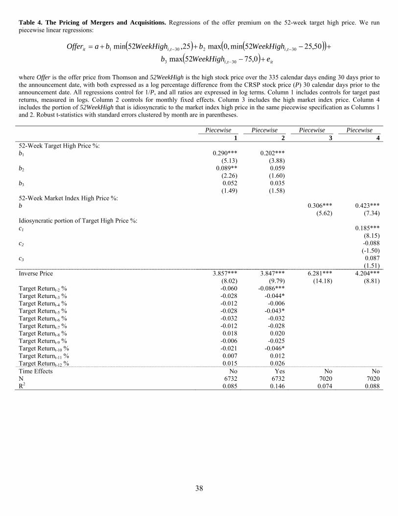
38

Table 4. The Pricing of Mergers and Acquisitions. Regressions of the offer premium on the 52-week target high price. We run piecewise linear regressions:

itti

titiit

eWeekHighb

WeekHighbWeekHighbaOffer

0,7552max

50,2552min,0max25,52min

30,3

30,230,1

where Offer is the offer price from Thomson and 52WeekHigh is the high stock price over the 335 calendar days ending 30 days prior to the announcement date, with both expressed as a log percentage difference from the CRSP stock price (P) 30 calendar days prior to the announcement date. All regressions control for 1/P, and all ratios are expressed in log terms. Column 1 includes controls for target past returns, measured in logs. Column 2 controls for monthly fixed effects. Column 3 includes the high market index price. Column 4 includes the portion of 52WeekHigh that is idiosyncratic to the market index high price in the same piecewise specification as Columns 1 and 2. Robust t-statistics with standard errors clustered by month are in parentheses. Piecewise Piecewise Piecewise Piecewise 1 2 3 4 52-Week Target High Price %: b1 0.290*** 0.202*** (5.13) (3.88) b2 0.089** 0.059 (2.26) (1.60) b3 0.052 0.035 (1.49) (1.58) 52-Week Market Index High Price %: b 0.306*** 0.423*** (5.62) (7.34) Idiosyncratic portion of Target High Price %: c1 0.185*** (8.15) c2 -0.088 (-1.50) c3 0.087 (1.51) Inverse Price 3.857*** 3.847*** 6.281*** 4.204*** (8.02) (9.79) (14.18) (8.81) Target Returnt-2 % -0.060 -0.086*** Target Returnt-3 % -0.028 -0.044* Target Returnt-4 % -0.012 -0.006 Target Returnt-5 % -0.028 -0.043* Target Returnt-6 % -0.032 -0.032 Target Returnt-7 % -0.012 -0.028 Target Returnt-8 % 0.018 0.020 Target Returnt-9 % -0.006 -0.025 Target Returnt-10 % -0.021 -0.046* Target Returnt-11 % 0.007 0.012 Target Returnt-12 % 0.015 0.026 Time Effects No Yes No No N 6732 6732 7020 7020 R2 0.085 0.146 0.074 0.088

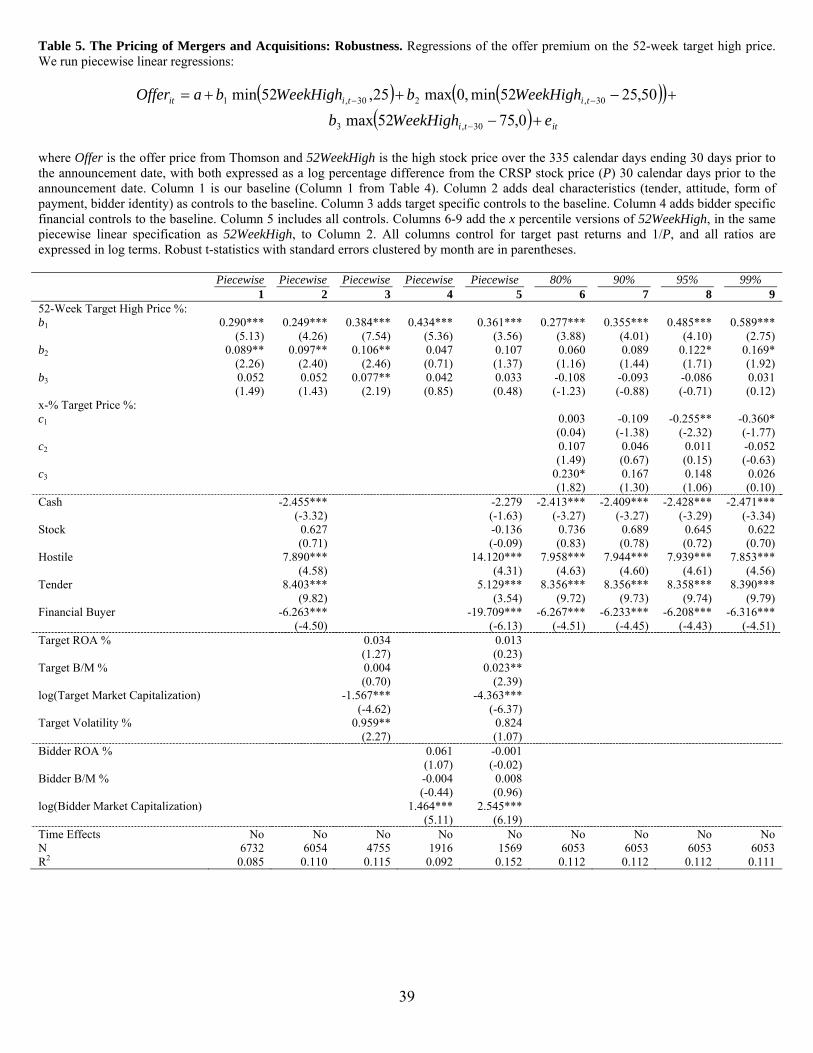
39

Table 5. The Pricing of Mergers and Acquisitions: Robustness. Regressions of the offer premium on the 52-week target high price. We run piecewise linear regressions:

itti

titiit

eWeekHighb

WeekHighbWeekHighbaOffer

0,7552max

50,2552min,0max25,52min

30,3

30,230,1

where Offer is the offer price from Thomson and 52WeekHigh is the high stock price over the 335 calendar days ending 30 days prior to the announcement date, with both expressed as a log percentage difference from the CRSP stock price (P) 30 calendar days prior to the announcement date. Column 1 is our baseline (Column 1 from Table 4). Column 2 adds deal characteristics (tender, attitude, form of payment, bidder identity) as controls to the baseline. Column 3 adds target specific controls to the baseline. Column 4 adds bidder specific financial controls to the baseline. Column 5 includes all controls. Columns 6-9 add the x percentile versions of 52WeekHigh, in the same piecewise linear specification as 52WeekHigh, to Column 2. All columns control for target past returns and 1/P, and all ratios are expressed in log terms. Robust t-statistics with standard errors clustered by month are in parentheses. Piecewise Piecewise Piecewise Piecewise Piecewise 80% 90% 95% 99% 1 2 3 4 5 6 7 8 9 52-Week Target High Price %: b1 0.290*** 0.249*** 0.384*** 0.434*** 0.361*** 0.277*** 0.355*** 0.485*** 0.589*** (5.13) (4.26) (7.54) (5.36) (3.56) (3.88) (4.01) (4.10) (2.75) b2 0.089** 0.097** 0.106** 0.047 0.107 0.060 0.089 0.122* 0.169* (2.26) (2.40) (2.46) (0.71) (1.37) (1.16) (1.44) (1.71) (1.92) b3 0.052 0.052 0.077** 0.042 0.033 -0.108 -0.093 -0.086 0.031 (1.49) (1.43) (2.19) (0.85) (0.48) (-1.23) (-0.88) (-0.71) (0.12) x-% Target Price %: c1 0.003 -0.109 -0.255** -0.360* (0.04) (-1.38) (-2.32) (-1.77) c2 0.107 0.046 0.011 -0.052 (1.49) (0.67) (0.15) (-0.63) c3 0.230* 0.167 0.148 0.026 (1.82) (1.30) (1.06) (0.10) Cash -2.455*** -2.279 -2.413*** -2.409*** -2.428*** -2.471*** (-3.32) (-1.63) (-3.27) (-3.27) (-3.29) (-3.34) Stock 0.627 -0.136 0.736 0.689 0.645 0.622 (0.71) (-0.09) (0.83) (0.78) (0.72) (0.70) Hostile 7.890*** 14.120*** 7.958*** 7.944*** 7.939*** 7.853*** (4.58) (4.31) (4.63) (4.60) (4.61) (4.56) Tender 8.403*** 5.129*** 8.356*** 8.356*** 8.358*** 8.390*** (9.82) (3.54) (9.72) (9.73) (9.74) (9.79) Financial Buyer -6.263*** -19.709*** -6.267*** -6.233*** -6.208*** -6.316*** (-4.50) (-6.13) (-4.51) (-4.45) (-4.43) (-4.51) Target ROA % 0.034 0.013 (1.27) (0.23) Target B/M % 0.004 0.023** (0.70) (2.39) log(Target Market Capitalization) -1.567*** -4.363*** (-4.62) (-6.37) Target Volatility % 0.959** 0.824 (2.27) (1.07) Bidder ROA % 0.061 -0.001 (1.07) (-0.02) Bidder B/M % -0.004 0.008 (-0.44) (0.96) log(Bidder Market Capitalization) 1.464*** 2.545*** (5.11) (6.19) Time Effects No No No No No No No No No N 6732 6054 4755 1916 1569 6053 6053 6053 6053 R2 0.085 0.110 0.115 0.092 0.152 0.112 0.112 0.112 0.111

40

Table 6. The Pricing of Mergers and Acquisitions: Subsamples. Piecewise linear regressions of the offer premium on the 52-week target high price, for subsamples. We divide the sample according to tender and non-tender offers, bidder attitude, and first and subsequent offers, successful and unsuccessful offers, form of payment, and first and second half of the sample period. All regressions control for 1/P, and all ratios are expressed in log terms. Robust t-statistics clustered by month are in parentheses.

Tender Attitude First Offer

No Yes – No Hostile Friendly –

Hostile No Yes – No 52-Week Target High Price %:

b1 0.216*** 0.332*** 0.311*** -0.026 0.298*** -0.101 (3.67) (6.26) (3.37) (-0.33) (5.25) (-1.22) b2 0.054 0.184** -0.013 0.120 0.081* 0.085 (1.22) (2.39) (-0.16) (1.33) (1.94) (0.83) b3 0.041 0.015 -0.040 0.098 0.054 -0.069 (1.03) (0.24) (-0.47) (1.15) (1.58) (-0.64) Inverse Price 4.040*** 3.845*** 3.854*** (8.65) (7.97) (8.03) Time Effects No No No N 6732 6732 6732 R2 0.101 0.086 0.085 Successful Form of Payment Second Half No Yes – No Stock Cash – Stock No Yes - No 52-Week Target High Price %:

b1 0.145* 0.191*** 0.402*** -0.137** 0.346*** -0.096* (1.87) (3.24) (5.29) (-2.03) (5.30) (-1.73) b2 0.075 0.054 -0.020 0.194** 0.085 0.015 (1.12) (0.73) (-0.23) (2.06) (1.44) (0.20) b3 0.079 -0.030 0.046 0.111* -0.007 0.077 (1.33) (-0.45) (0.87) (1.67) (-0.09) (1.01) Inverse Price 4.251*** 4.134*** 3.825*** (8.36) (6.60) (7.96) Time Effects No No No N 6208 4450 6732 R2 0.105 0.092 0.086

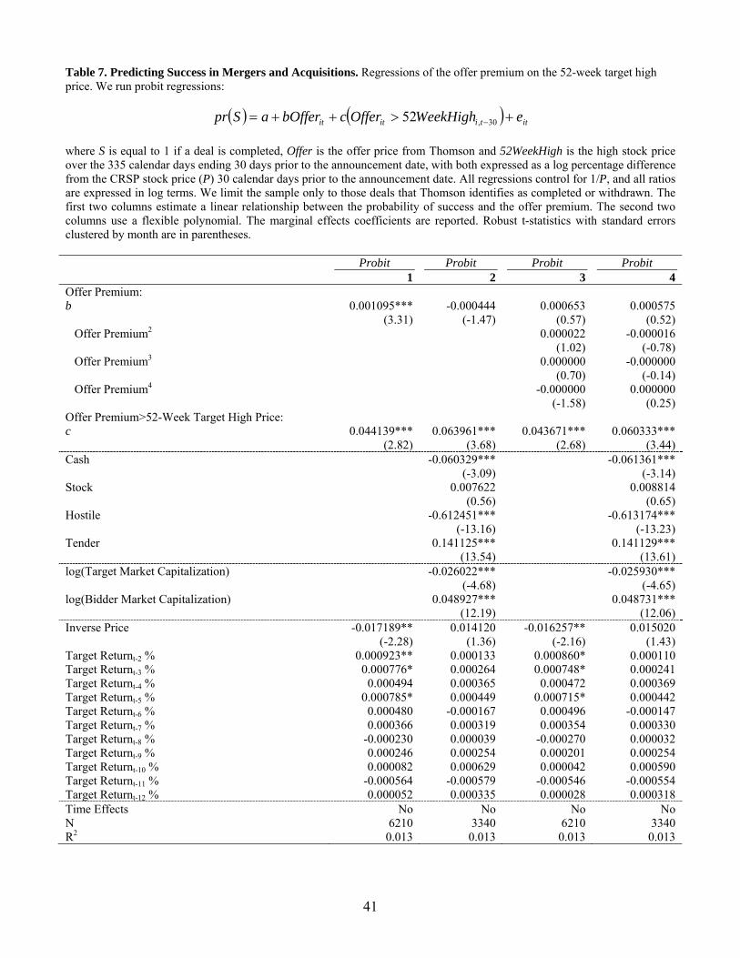
41

Table 7. Predicting Success in Mergers and Acquisitions. Regressions of the offer premium on the 52-week target high price. We run probit regressions:

ittiitit eWeekHighOffercbOfferaSpr 30,52

where S is equal to 1 if a deal is completed, Offer is the offer price from Thomson and 52WeekHigh is the high stock price over the 335 calendar days ending 30 days prior to the announcement date, with both expressed as a log percentage difference from the CRSP stock price (P) 30 calendar days prior to the announcement date. All regressions control for 1/P, and all ratios are expressed in log terms. We limit the sample only to those deals that Thomson identifies as completed or withdrawn. The first two columns estimate a linear relationship between the probability of success and the offer premium. The second two columns use a flexible polynomial. The marginal effects coefficients are reported. Robust t-statistics with standard errors clustered by month are in parentheses. Probit Probit Probit Probit 1 2 3 4 Offer Premium: b 0.001095*** -0.000444 0.000653 0.000575 (3.31) (-1.47) (0.57) (0.52) Offer Premium2 0.000022 -0.000016 (1.02) (-0.78) Offer Premium3 0.000000 -0.000000 (0.70) (-0.14) Offer Premium4 -0.000000 0.000000 (-1.58) (0.25) Offer Premium>52-Week Target High Price: c 0.044139*** 0.063961*** 0.043671*** 0.060333*** (2.82) (3.68) (2.68) (3.44) Cash -0.060329*** -0.061361*** (-3.09) (-3.14) Stock 0.007622 0.008814 (0.56) (0.65) Hostile -0.612451*** -0.613174*** (-13.16) (-13.23) Tender 0.141125*** 0.141129*** (13.54) (13.61) log(Target Market Capitalization) -0.026022*** -0.025930*** (-4.68) (-4.65) log(Bidder Market Capitalization) 0.048927*** 0.048731*** (12.19) (12.06) Inverse Price -0.017189** 0.014120 -0.016257** 0.015020 (-2.28) (1.36) (-2.16) (1.43) Target Returnt-2 % 0.000923** 0.000133 0.000860* 0.000110 Target Returnt-3 % 0.000776* 0.000264 0.000748* 0.000241 Target Returnt-4 % 0.000494 0.000365 0.000472 0.000369 Target Returnt-5 % 0.000785* 0.000449 0.000715* 0.000442 Target Returnt-6 % 0.000480 -0.000167 0.000496 -0.000147 Target Returnt-7 % 0.000366 0.000319 0.000354 0.000330 Target Returnt-8 % -0.000230 0.000039 -0.000270 0.000032 Target Returnt-9 % 0.000246 0.000254 0.000201 0.000254 Target Returnt-10 % 0.000082 0.000629 0.000042 0.000590 Target Returnt-11 % -0.000564 -0.000579 -0.000546 -0.000554 Target Returnt-12 % 0.000052 0.000335 0.000028 0.000318 Time Effects No No No No N 6210 3340 6210 3340 R2 0.013 0.013 0.013 0.013

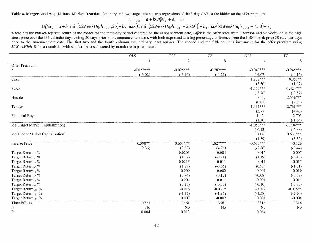
42

Table 8. Mergers and Acquisitions: Market Reaction. Ordinary and two-stage least squares regressions of the 3-day CAR of the bidder on the offer premium:

itittt ebOfferar 11 and

ittititiit eWeekHighbWeekHighbWeekHighbaOffer 0,7552max50,2552min,0max25,52min 30,330,230,1

where r is the market-adjusted return of the bidder for the three-day period centered on the announcement date, Offer is the offer price from Thomson and 52WeekHigh is the high stock price over the 335 calendar days ending 30 days prior to the announcement date, with both expressed as a log percentage difference from the CRSP stock price 30 calendar days prior to the announcement date. The first two and the fourth columns use ordinary least squares. The second and the fifth columns instrument for the offer premium using 52WeekHigh. Robust t-statistics with standard errors clustered by month are in parentheses. OLS OLS IV OLS IV 1 2 3 4 5 Offer Premium: b -0.022*** -0.025*** -0.282*** -0.040*** -0.245*** (-3.02) (-3.16) (-4.21) (-4.67) (-4.15) Cash 1.232*** 0.851** (3.50) (1.97) Stock -1.373*** -1.424*** (-3.76) (-3.57) Hostile 0.557 2.556*** (0.81) (2.63) Tender 1.431*** 2.768*** (3.77) (4.46) Financial Buyer 1.424 -2.703 (1.30) (-1.64) log(Target Market Capitalization) -1.053*** -1.704*** (-6.13) (-5.88) log(Bidder Market Capitalization) 0.140 0.631*** (1.39) (3.32) Inverse Price 0.390** 0.651*** 1.827*** -0.630*** -0.126 (2.36) (3.63) (4.76) (-2.86) (-0.44) Target Returnt-2 % 0.020* -0.004 0.015 -0.007 Target Returnt-3 % (1.67) (-0.24) (1.19) (-0.43) Target Returnt-4 % 0.021* -0.011 0.011 -0.017 Target Returnt-5 % (1.89) (-0.66) (0.95) (-1.01) Target Returnt-6 % 0.009 0.002 -0.001 -0.010 Target Returnt-7 % (0.74) (0.12) (-0.08) (-0.67) Target Returnt-8 % 0.004 -0.011 -0.001 -0.015 Target Returnt-9 % (0.27) (-0.70) (-0.10) (-0.95) Target Returnt-10 % -0.016 -0.031* -0.022 -0.035** Target Returnt-11 % (-1.17) (-1.95) (-1.58) (-2.20) Target Returnt-12 % 0.007 -0.002 0.001 -0.008 Time Effects 3723 3561 3561 3316 3316 N No No No No No R2 0.004 0.013 . 0.064 .

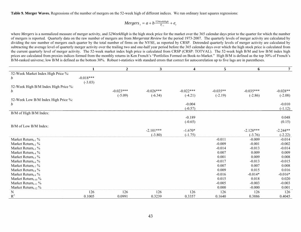
43

Table 9. Merger Waves. Regressions of the number of mergers on the 52-week high of different indices. We run ordinary least squares regressions:

tPWeekHigh

t ebaMergerst

1

52

where Mergers is a normalized measure of merger activity, and 52WeekHigh is the high stock price for the market over the 365 calendar days prior to the quarter for which the number of mergers is reported. Quarterly data on the raw number of mergers are from Mergerstat Review for the period 1973-2007. The quarterly levels of merger activity are calculated by dividing the raw number of mergers each quarter by the total number of firms on the NYSE, as reported by CRSP. Detrended quarterly levels of merger activity are calculated by subtracting the average level of quarterly merger activity over the trailing two and one-half year period before the 365 calendar days over which the high stock price is calculated from the current quarterly level of merger activity. The 52-week market index high price is calculated from CRSP (CRSP: TOTVAL). The 52-week high B/M and low B/M index high prices are calculated from proxies indices formed from the monthly returns in Ken French’s “Portfolios Formed on Book-to-Market.” High B/M is defined as the top 30% of French’s B/M-ranked universe; low B/M is defined as the bottom 30%. Robust t-statistics with standard errors that correct for autocorrelation up to five lags are in parentheses. 1 2 3 4 5 6 7 52-Week Market Index High Price %: b -0.018*** (-3.03) 52-Week High B/M Index High Price %: b -0.023*** -0.026*** -0.022*** -0.035** -0.035*** -0.028** (-5.09) (-6.34) (-4.21) (-2.19) (-2.86) (-2.08) 52-Week Low B/M Index High Price %: b -0.004 -0.010 (-0.57) (-1.12) B/M of High B/M Index: -0.189 0.048 (-0.65) (0.15) B/M of Low B/M Index:

-2.101*** -1.670* -2.128*** -2.244** (-3.80) (-1.75) (-3.76) (-2.22)

Market Returnt-1 % -0.011 -0.009 -0.014 Market Returnt-2 % -0.009 -0.001 -0.002 Market Returnt-3 % -0.014 -0.013 -0.014 Market Returnt-4 % 0.007 0.009 0.009 Market Returnt-5 % 0.001 0.009 0.008 Market Returnt-6 % -0.017 -0.013 -0.015 Market Returnt-7 % 0.007 0.007 0.008 Market Returnt-8 % 0.009 0.015 0.016 Market Returnt-9 % -0.016 -0.014* -0.016* Market Returnt-10 % 0.015 0.018 0.020 Market Returnt-11 % -0.005 -0.003 -0.003 Market Returnt-12 % 0.000 -0.000 0.001 N 126 126 126 126 126 126 126 R2 0.1005 0.0991 0.3239 0.3357 0.1640 0.3886 0.4045

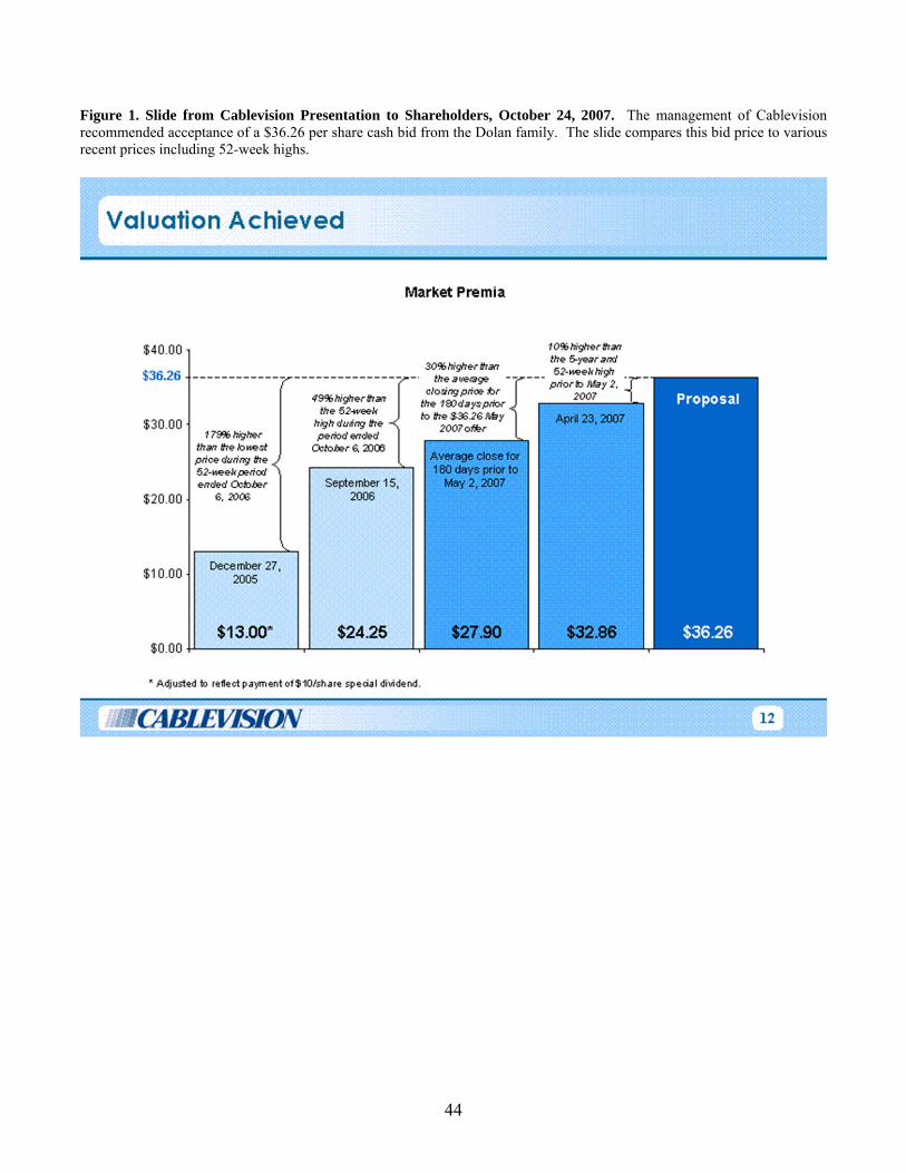
44

Figure 1. Slide from Cablevision Presentation to Shareholders, October 24, 2007. The management of Cablevision recommended acceptance of a $36.26 per share cash bid from the Dolan family. The slide compares this bid price to various recent prices including 52-week highs.

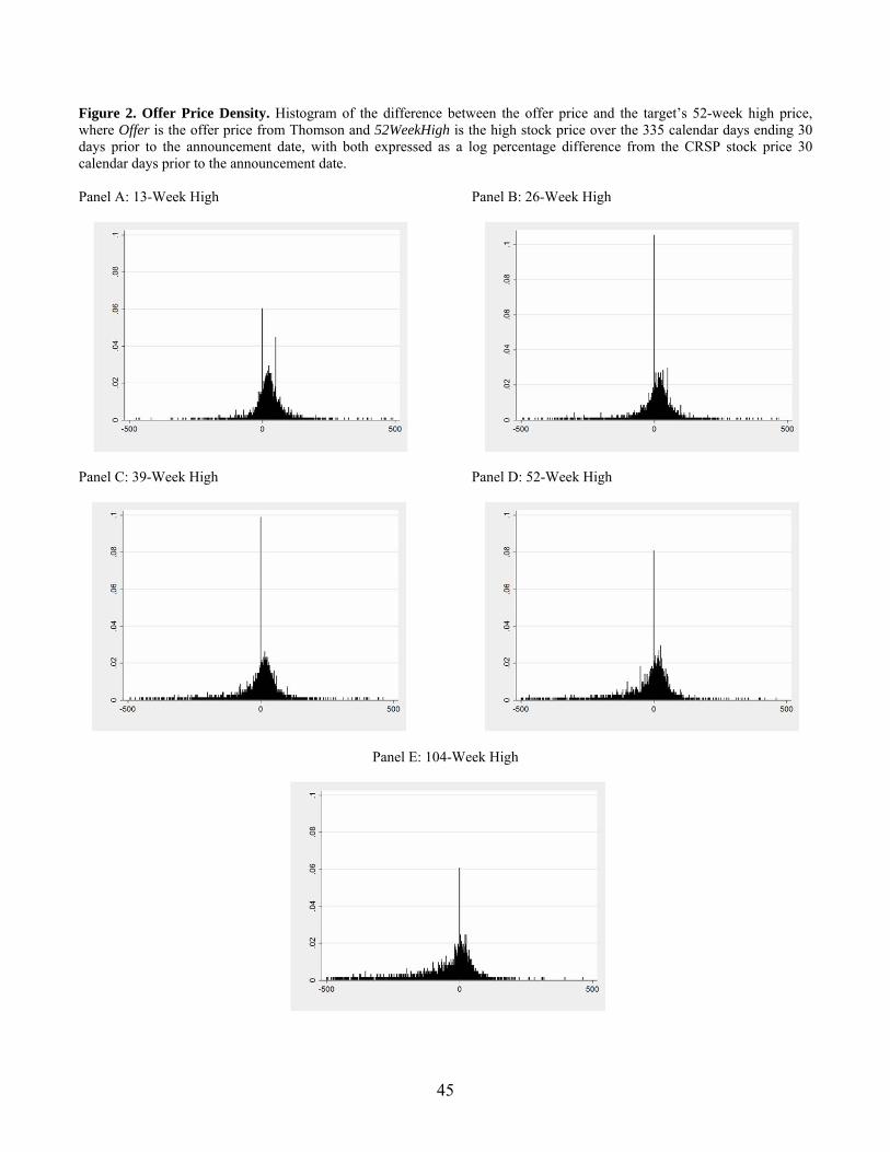
45

Figure 2. Offer Price Density. Histogram of the difference between the offer price and the target’s 52-week high price, where Offer is the offer price from Thomson and 52WeekHigh is the high stock price over the 335 calendar days ending 30 days prior to the announcement date, with both expressed as a log percentage difference from the CRSP stock price 30 calendar days prior to the announcement date.

Panel A: 13-Week High

Panel C: 39-Week High

Panel B: 26-Week High

Panel D: 52-Week High

Panel E: 104-Week High

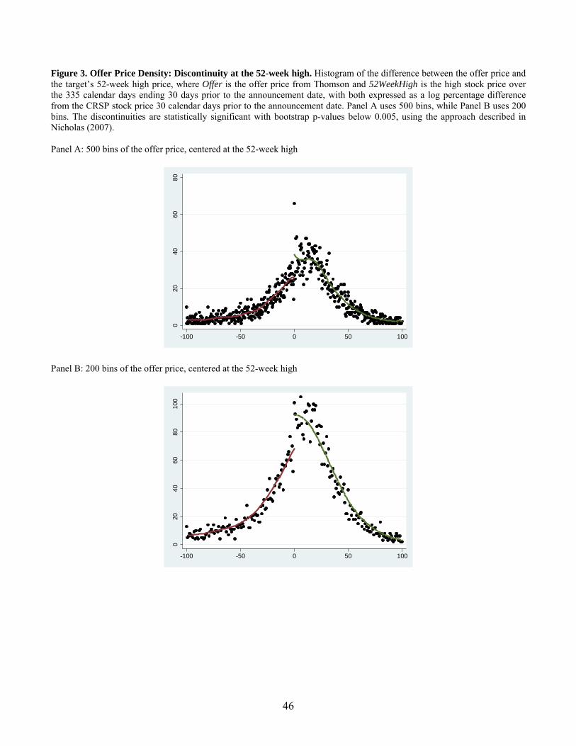
46

Figure 3. Offer Price Density: Discontinuity at the 52-week high. Histogram of the difference between the offer price and the target’s 52-week high price, where Offer is the offer price from Thomson and 52WeekHigh is the high stock price over the 335 calendar days ending 30 days prior to the announcement date, with both expressed as a log percentage difference from the CRSP stock price 30 calendar days prior to the announcement date. Panel A uses 500 bins, while Panel B uses 200 bins. The discontinuities are statistically significant with bootstrap p-values below 0.005, using the approach described in Nicholas (2007). Panel A: 500 bins of the offer price, centered at the 52-week high

Panel B: 200 bins of the offer price, centered at the 52-week high

020

4060

80

-100 -50 0 50 100

020

4060

8010

0

-100 -50 0 50 100

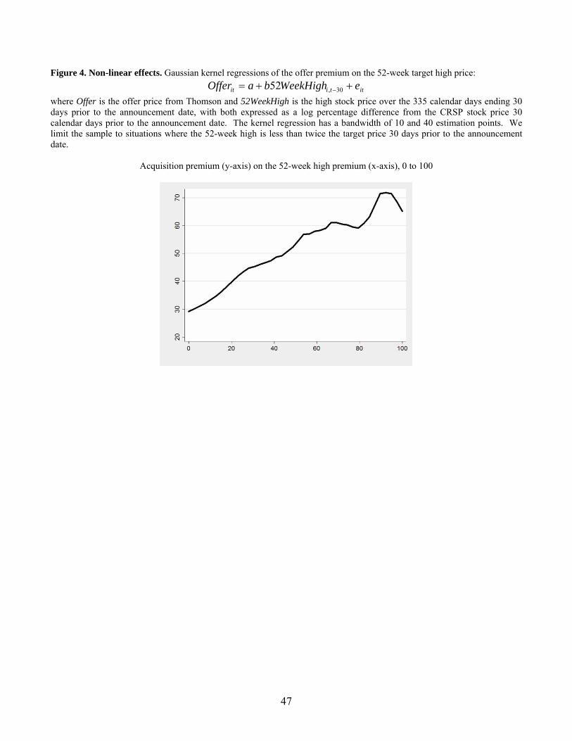
47

Figure 4. Non-linear effects. Gaussian kernel regressions of the offer premium on the 52-week target high price:

ittiit eWeekHighbaOffer 30,52

where Offer is the offer price from Thomson and 52WeekHigh is the high stock price over the 335 calendar days ending 30 days prior to the announcement date, with both expressed as a log percentage difference from the CRSP stock price 30 calendar days prior to the announcement date. The kernel regression has a bandwidth of 10 and 40 estimation points. We limit the sample to situations where the 52-week high is less than twice the target price 30 days prior to the announcement date.

Acquisition premium (y-axis) on the 52-week high premium (x-axis), 0 to 100

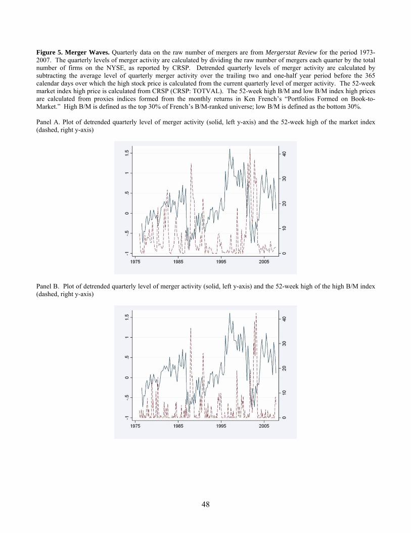
48

Figure 5. Merger Waves. Quarterly data on the raw number of mergers are from Mergerstat Review for the period 1973-2007. The quarterly levels of merger activity are calculated by dividing the raw number of mergers each quarter by the total number of firms on the NYSE, as reported by CRSP. Detrended quarterly levels of merger activity are calculated by subtracting the average level of quarterly merger activity over the trailing two and one-half year period before the 365 calendar days over which the high stock price is calculated from the current quarterly level of merger activity. The 52-week market index high price is calculated from CRSP (CRSP: TOTVAL). The 52-week high B/M and low B/M index high prices are calculated from proxies indices formed from the monthly returns in Ken French’s “Portfolios Formed on Book-to-Market.” High B/M is defined as the top 30% of French’s B/M-ranked universe; low B/M is defined as the bottom 30%. Panel A. Plot of detrended quarterly level of merger activity (solid, left y-axis) and the 52-week high of the market index (dashed, right y-axis)

Panel B. Plot of detrended quarterly level of merger activity (solid, left y-axis) and the 52-week high of the high B/M index (dashed, right y-axis)