Embed Size (px)
Citation preview

Accepted Manuscript
The effect of real earnings management on the persistence and informativeness ofearnings
Valerie Li
PII: S0890-8389(19)30027-7
DOI: https://doi.org/10.1016/j.bar.2019.02.005
Reference: YBARE 823
To appear in: The British Accounting Review
Received Date: 27 April 2017
Revised Date: 8 February 2019
Accepted Date: 14 February 2019
Please cite this article as: Li, V., The effect of real earnings management on the persistence andinformativeness of earnings, The British Accounting Review (2019), doi: https://doi.org/10.1016/j.bar.2019.02.005.
This is a PDF file of an unedited manuscript that has been accepted for publication. As a service toour customers we are providing this early version of the manuscript. The manuscript will undergocopyediting, typesetting, and review of the resulting proof before it is published in its final form. Pleasenote that during the production process errors may be discovered which could affect the content, and alllegal disclaimers that apply to the journal pertain.

MANUSCRIP
T
ACCEPTED
ACCEPTED MANUSCRIPT
The Effect of Real Earnings Management on the Persistence and Informativeness
of Earnings
Valerie Li
University of Washington Bothell
Email: [email protected]
February 7, 2019
Abstract: This study investigates the effect of real earnings management on two important aspects
of earnings quality: earnings persistence and its informativeness about future cash flows. I focus
on real earnings management through the abnormal reduction in discretionary expenditures and
investigate how this type of real earnings management affects earnings quality. Examining a large
sample over a period of four decades, I find that the extent of real earnings management is
negatively related to earnings persistence, and this effect is achieved largely through the negative
effect of real earnings management on cash flows rather than on accruals. The less persistent
current earnings as a result of real earnings management exhibit a weakened ability to predict
future cash flows, suggesting a decreased informativeness of current earnings about future cash
flows. Moreover, I find that the negative effect of the abnormal reduction in discretionary expenses
on earnings persistence and its association with future cash flows from operations is more
pronounced in the post-SOX period. Overall, the results suggest that real earnings management
through the abnormal reduction in discretionary expenses is associated with deteriorated earnings
quality.
Keywords: real earnings management; abnormal reduction in discretionary expenses; cash flow
manipulation; R&D; advertising expenses; earnings persistence; earnings quality;
JEL classifications: G31; M40; M41;
I would like to thank Zhiyan Cao, Matt Cedergren, Rajib Doogar, Weili Ge, Adam Greiner, Steve Holland,
Nathan L. Joseph (editor), Alan Lowe (editor), Terry Shevlin, D. Shores, Ron Tilden, Ryan Wilson, Jenny
Zhang, Hong Zou (associate editor), two anonymous reviewers, workshop participants at China Europe
International Business School, Wuhan University, University of Washington, and University of
Washington Bothell, as well as participants at the 2018 American Accounting Association Annual Meeting
and 2018 Western Region Conference for helpful comments.

MANUSCRIP
T
ACCEPTED
ACCEPTED MANUSCRIPT
The Effect of Real Earnings Management on the Persistence and Informativeness of Earnings
Abstract: This study investigates the effect of real earnings management on two important aspects of earnings quality: earnings persistence and its informativeness about future cash flows. I focus on real earnings management through the abnormal reduction in discretionary expenditures and investigate how this type of real earnings management affects earnings quality. Examining a large sample over a period of four decades, I find that the extent of real earnings management is negatively related to earnings persistence, and this effect is achieved largely through the negative effect of real earnings management on cash flows rather than on accruals. The less persistent current earnings as a result of real earnings management exhibit a weakened ability to predict future cash flows, suggesting a decreased informativeness of current earnings about future cash flows. Moreover, I find that the negative effect of the abnormal reduction in discretionary expenses on earnings persistence and its association with future cash flows from operations is more pronounced in the post-SOX period. Overall, the results suggest that real earnings management through the abnormal reduction in discretionary expenses is associated with deteriorated earnings quality.

MANUSCRIP
T
ACCEPTED
ACCEPTED MANUSCRIPT
1
1. Introduction
Prior literature provides evidence on the existence of real earnings management
(Roychowdhury, 2006; Cohen et al., 2008). This type of earnings management alters firms’ real
operations and have potentially long-term operating consequences (Graham et al., 2005).
Surprisingly, despite the prevalence of real earnings management, little research addresses how
real earnings management affects earning quality. DeFond (2010, 406) points out that “…we
know little about whether or how transactions management impacts EQ” and that “transaction
management seems like an important area for further research.” To answer this call, I investigate
whether real earnings management influences earnings persistence and its informativeness about
future cash flows (two widely used measures of earnings quality) and whether the influence on
earnings persistence is equal across cash flow and accrual components of earnings. My study is
the first to provide large-sample empirical evidence on this issue. Following prior literature
(Hanlon, 2005; Atwood et al., 2010), I assume that higher persistence reflects higher earnings
quality because earnings that possess such properties are viewed by investors as more sustainable,
more permanent and less transitory, and, therefore, generally preferable.1 Similarly, a stronger
association between current earnings and future cash flows indicates the greater ability of current
earnings to forecast future cash flows.
Real earnings management can appear in many forms.2 I focus my investigation on one
form of real earnings management — the abnormal reduction in discretionary expenses — for
1 I acknowledge that earnings with high persistence are not always of high quality when underlying economic earnings are volatile. Earnings quality contains many attributes and is not fully captured by one particular attribute. I build on prior literature that considers higher persistence to be of higher earnings quality to conduct my analysis (e.g., Hanlon, 2005; Li, 2008; Atwood et al., 2010). 2 Other forms of real earnings management include accelerating the timing of production, offering a suboptimal price discount, altering investing (e.g., sales of assets), and financing activities (e.g., stock repurchases).

MANUSCRIP
T
ACCEPTED
ACCEPTED MANUSCRIPT
2
the following two reasons.3 First, based on the survey report of financial executives conducted by
Graham et al. (2005), the abnormal reduction of discretionary expenses is a more pervasive and
preferred form of real earnings management that managers use to boost earnings. Second, the
abnormal reduction in discretionary expenses provides a cleaner setting to investigate the effect
of real earnings management on earnings quality. Real earnings management has different
implications for profit margin and operating cash flows, depending on the specific forms of real
earnings management (Kothari et al., 2016). Abnormal reductions in discretionary expenses,
such as research and development (R&D), advertising, and selling, general, and administration
(SG&A), can temporarily increase current earnings and enable a firm to have higher profit
margins and operating cash flows. However, other forms of real earnings management, such as
price discounts and overproduction, could overstate earnings but simultaneously decrease profit
margins and cash flows from operations (Roychowdhury, 2006; Kothari et al., 2016). When cash
flows from operations are abnormally low in the current period while earnings are artificially
overstated, low current-period cash flow from operations could reverse and return to the normal
level in the future, exhibiting low persistence. At the same time, earnings continue to be high in
the next period, exhibiting high persistence. Hence, unlike the abnormal reduction in
discretionary expenses, the effect of price discounts and overproduction on earnings persistence
is ambiguous.
The first research question I address is whether and how real earnings management
through the abnormal reduction in discretionary expenses affects earnings persistence.
Depending on different managerial incentives, earnings management can affect earnings
persistence differently. On the one hand, firms can use real earnings management to
3 I follow prior literature to use the terminology “abnormal reduction in discretionary expenses” to define managers’ actions to reduce these variable expenses below a normal level in the current period to boost earnings (Roychowdhury, 2006; Cheng et al., 2016).

MANUSCRIP
T
ACCEPTED
ACCEPTED MANUSCRIPT
3
opportunistically increase current reported earnings and, in turn, reduce earnings persistence; this
is because artificially increased current earnings will not persist into the future. On the other
hand, firms can use real earnings management to smooth earnings or signal future profitability.
As a result, current period earnings, although managed upward, will persist to a future period.4
Prior literature provides evidence that managers reduce discretionary expenditures such as R&D
expenditures (Baber et al., 1991; Dechow & Sloan, 1991), advertising expenses (Mizik &
Jacobson, 2007), and SG&A expenses (Roychowdury, 2006) below normal levels to improve
current earnings and meet certain earnings goals. These findings are consistent with the abnormal
reduction in discretionary expenditures being used to improve current earnings rather than to
smooth earnings. Prior studies also examine the signaling theory of real earnings management,
but the empirical evidence is inconclusive. The evidence suggests that, in some cases, managers
may use real earnings management to signal positive future performance (Gunny, 2010), but in
other cases, real earnings management is associated with lower future performance (Cheng et al.,
2016; Mizik & Jacobson, 2007). Theoretically, as firms’ positive net present value (NPV)
projects are funded by the normal level of R&D, advertising, and SG&A expenses, increasing
current period earnings through cutting these discretionary expenditures below normal levels is
achieved at the cost of forgoing firms’ future economic benefit and long-term value. Hence, at
the conceptual level, such reduction is more likely to be detrimental to future performance. To
the extent that managers do not engage in the abnormal reduction in discretionary expenditures
permanently, I conjecture that earnings persistence is decreased by the abnormal reduction in
discretionary expenditures. Using a sample of US firms from 1975 to 2016, I find that when real
earnings management is measured through cutting discretionary expenditures (Roychowdhury,
4 I thank an anonymous referee for suggesting this alternative explanation.

MANUSCRIP
T
ACCEPTED
ACCEPTED MANUSCRIPT
4
2006; Cohen et al., 2008; Cheng et al., 2016), the persistence of current earnings decreases with
my measure of real earnings management.
Next, I investigate whether the impact of the abnormal reduction in discretionary
expenses on earnings persistence is through its impact on the accruals or cash flows from
operations. As discretionary expenses are generally in the form of cash, a reduction in
discretionary expenses could lower cash outflows and increase net cash flows from operations in
the current period (Bushee, 1998; Roychowdhury, 2006; Lee, 2012). I conjecture that cash flows
are more likely to be affected by real earnings management. To test this conjecture, I decompose
current earnings into accruals and cash flows from operations. I find that the persistence of cash
flows significantly decreases in all cases of the discretionary expense reductions but the
persistence of accruals remains unchanged in the cases of real earnings management through the
abnormal reduction in R&D, advertising, and total discretionary expense. My results suggest that
the impact of real earnings management through the abnormal reduction in discretionary
expenditures on earnings persistence largely comes from its negative impact on the persistence
of cash flows from operations.
My third analysis focuses on whether real earnings management affects the
informativeness of current earnings about future cash flows. Earnings persistence measures the
portion of current earnings that persists to future earnings and is related to the usefulness of
earnings (Shipper & Vincent, 2003). Highly persistent earnings numbers should be more
informative about and highly associated with future cash flows. Since real earnings management
through the abnormal reduction in discretionary expenses reduces earnings persistence, it may
affect the association between current earnings and future cash flows. Consistent with this notion,

MANUSCRIP
T
ACCEPTED
ACCEPTED MANUSCRIPT
5
my results show that the abnormal reduction in discretionary expenses significantly decreases the
ability of current earnings in predicting future cash flows.
Motivated by the trend of increased use of real earnings management after the passage of
the Sarbanes Oxley Act (SOX) (Cohen et al., 2008), I hypothesize that the effect of the abnormal
reduction in discretionary expenses on earnings quality is more pronounced in the post-SOX
period.5 My results are generally consistent with this conjecture.
I conduct a battery of additional tests to increase the validity of my findings. First, I find
some evidence that the negative effect of real earnings management through the abnormal
reduction of discretionary expenses is stronger when firms engage in activities to meet or just
beat earnings targets. Second, I control for accruals earnings management and find that real
earnings management through the abnormal reduction in discretionary expenses has an
incremental negative effect on the persistence and informativeness of current earnings beyond
the effect of accruals earnings management. Third, I use alternative real earnings management
measures and alternative model specifications. My results are robust to these different
approaches. Finally, my inferences do not change when I use different samples, industry
classifications, and variable measurement.
This paper makes two important contributions to the existing literature. First, it
contributes to the literature on earnings quality. Prior research investigates differential
persistence of earnings components and finds that the discretionary accruals component of
earnings is less persistent than other components of earnings (e.g., both normal accruals and cash
from operations, Xie, 2001). This stream of literature compares the persistence of different
earnings components but contains few studies that examine whether managing components of
5 I thank an anonymous referee for suggesting this set of tests.
MANUSCRIP
T
ACCEPTED
ACCEPTED MANUSCRIPT
6
earnings affects the overall persistence of earnings.6 My study fills this gap by directly assessing
how real earnings management, one type of earnings management that can affect both the
accrual and cash flow components of earnings, affect earnings persistence. If firms manage
earnings, either through real earnings management or through accrual earnings management, to
smooth earnings, then earnings persistence would increase; if firms manage earnings to
temporarily increase reported earnings, current period earnings could become less persistent.7
Further, if managers manage earnings to communicate private information about firms’ future
profitability — the signaling theory of earnings management — earnings persistence can also be
increased. Therefore, although earnings management in general is a temporary decision by
managers, the effect of different types of earnings management, on earnings persistence in
particular and earnings quality in general, is not clear ex ante. By providing direct evidence that
the abnormal reduction in discretionary expenditures affects the persistence and informativeness
of current earnings, my study is the first to answer Defond’s (2010) call for more research on real
earnings management, and advances our understanding of how real transaction management
affects earnings quality. Although earnings management may result in more or less persistent
earnings, my empirical results show that real earnings management through the abnormal
reduction in discretionary expenditures, on average, reduces earnings persistence and current
earnings’ informativeness of future cash flows. To mitigate the concern that the negative effect
of real earnings management on earnings quality is driven by accrual earnings management, in
the sensitivity tests in Section 4.5, I control for the effect of accruals management and find that
6 A notable exception is the study of DeChow and Dichev (2002) that provides evidence that accruals of poor quality, measured by their AQ measure, are associated with earnings with lower persistence. 7 Real earnings management and accrual earnings management can both affect firms’ total accruals, but their effects on certain types of accruals are fundamentally different. For example, real earnings management through cutting discretionary expenditures more likely affect accrual accounts that rely less on management’s estimate (e.g., accounts payable), while accrual earnings management are more likely to affect accrual accounts that are more subject to managers’ estimate (e.g., allowance for doubtful accounts). How each type of accruals is affected by different earnings management mechanisms is beyond the scope of this paper and is left to future research.

MANUSCRIP
T
ACCEPTED
ACCEPTED MANUSCRIPT
7
real earnings management has incremental effects on earnings quality beyond the effect of
accrual management.
Second, this paper contributes to the earnings management literature. Earnings consist of
two components, accruals and cash flows. Extant research in earnings management largely
focuses on accruals earnings management, implicitly assuming cash flows are free of
manipulation (e.g., Francis et al., 2005). However, my findings suggest that this is not always
the case. I show that real earnings management through the abnormal reduction in discretionary
expenses negatively reduces the quality of cash flows from operations, and that such effect, in
turn, reduces the persistence and informativeness of current earnings. The negative effect of real
earnings management arises because both accruals and cash flows are subject to manipulation in
the presence of real earnings management and hence examining the quality of both earnings
components in empirical studies provides more confident conclusions. My findings suggest that
researchers should consider both accrual and real earnings management when conducting
earnings management research.
The remainder of the paper proceeds as follows. Section 2 presents an overview of the
related literature and develops hypotheses. Section 3 describes the sample, data, and research
design. Section 4 discusses the empirical methodology and analyzes the results. Section 5
concludes the study.
2. Related research and hypotheses development
Following prior literature (Roychowdhury, 2006; Gunny, 2010), I define real earnings
management as management actions that deviate from normal business practices, undertaken
with the primary objective of influencing current period earnings. By altering underlying

MANUSCRIP
T
ACCEPTED
ACCEPTED MANUSCRIPT
8
operations, firms that engage in real earnings management influence current period earnings at
the cost of future economic value. Real earnings management has gained increasing attention in
accounting research. Graham et al. (2005) survey 401 financial executives and report that 78% of
the executives interviewed are willing to sacrifice economic value (such as reducing R&D,
advertising, and maintenance expenditures) to manage financial reporting perceptions. Cohen et
al. (2008) document that real earnings management increased significantly after the passage of
SOX in 2002. I focus my study on firm’s discretionary expense choices because prior research
suggests that discretionary expense manipulations are an important and pervasive form of real
earnings management (Kothari et al., 2016; Graham et al., 2005).
Several different incentives can be at play when firms choose to use real earnings
management to manage earnings. Specifically, firms can use real earnings management to
opportunistically increase reported earnings in the current period, to smooth earnings, or to
signal future profitability. In the case of abnormal reductions in discretionary expenditures,
accounting treatment allows such reductions to mechanically increase current-period reported
earnings. Prior studies provide evidence that managers cut discretionary expenses below normal
levels to meet earnings targets or financing goals. For example, Roychowdhury (2006) shows
that firms use reductions in discretionary expenses to increase current reported earnings. Perry
and Grinaker (1994) find evidence consistent with R&D expenditures being adjusted to meet
firms’ current earnings goals. Baber et al. (1991) show that managers are more likely to reduce
their investments in R&D when such reductions help them meet current period earnings targets.
Mizik and Jacobson (2007) find that firms that report higher earnings have lower-than-normal
marketing expenses at the time of seasonal equity offering, suggesting that these firms are
managing marketing expenses to boost current earnings. Roychowdhury (2006) points out that
MANUSCRIP
T
ACCEPTED
ACCEPTED MANUSCRIPT
9
SG&A often include discretionary expenses such as employee training, maintenance, and travel
etc., which can be reduced to meet earnings targets.8 Collectively, these findings indicate that
firms reduce R&D, advertising, and SG&A expenditures more likely to boost current reported
earnings rather than to smooth earnings. Hence, earnings of firms engaging in this type of real
earnings management are likely to become less persistent.
The signaling theory of accruals earnings management suggests that managers can
manage earnings to communicate private information about future profitability that is not
reflected in historical cost accounting and to signal firms’ future performance (Subramnayam,
1996) — a line of argument that could be extended to real earnings management. If managers
use real earnings management to convey private information and signal future positive
profitability, real earnings management is expected to be positively correlated with future
performance. Prior studies provide inconclusive evidence on whether managers use real earnings
management as a way to signal future performance. Gunny (2010) finds that firms engaging in
real earnings management to meet or just beat benchmarks have better subsequent performance.
However, Cheng et al. (2016) find that their measure of real earnings management is
significantly associated with lower future returns on assets and cash flows from operations.
Mizik and Jacobson (2007) find that firms that cut marketing spending in the seasonal equity
offering context have inferior long-term stock market performance.9 The empirical evidence in
prior literature suggests that it is possible that, in some cases, managers may use real earnings
8 Roychowdhury (2006) also finds evidence that managers use price discounts to temporarily increase sales and overproduction to report lower cost of goods sold to improve reported earnings. Because this paper does not intend to analyze every possible type of real earnings management, I focus on investigating managers’ decisions to reduce discretionary expenses below normal levels. 9 In an untabulated analysis, I also find mixed results on the association between real earnings management measures and subsequent industry-adjusted ROA (the proxy for performance in Gunny, 2010). However, I find a consistent negative association between real earnings management and subsequent unadjusted earnings, which is consistent with the findings of Cheng et al. (2016). I also find consistent evidence on the negative effect of real earnings management on earnings persistence when using unadjusted earnings.

MANUSCRIP
T
ACCEPTED
ACCEPTED MANUSCRIPT
10
management to signal positive future performance and, hence, the increased earnings in the
current period may persist into future periods. However, theoretically, compared to accruals
earnings management, real earnings management is more costly and more detrimental to firms’
operations. To engage in real earnings management, managers have to pass positive NPV
projects that are originally funded by the normal level of R&D, advertising, and SG&A
expenditures. Passing positive NPV projects will harm firms’ future performance.10 Therefore, at
the conceptual level, real earnings management achieved through the abnormal reduction in
discretionary expenses by reducing positive NPV projects in the current period, probably is more
likely to be detrimental to future performance. Based on the above discussion, I posit that:
H1: The extent of real earnings management through the abnormal reduction in
discretionary expenses is negatively associated with earnings persistence.
Discretionary expenses are generally in the form of cash, although, in some cases, can also
be in the form of accruals. Roychowdhury (2006) points out that reducing these expenses lowers
cash outflows and affects cash flows from operations in the current period. Bushee (1998) finds
evidence that firms with cash constraints are more likely to cut R&D to manage earnings,
indicating that cutting R&D increases firms’ cash flows from operations in the current period.
Lee (2012) also points out that reducing discretionary expenditures has a positive effect on
current period cash flows from operations. To the extent that discretionary expenses are more
likely in the form of cash than accruals, real earnings management through the abnormal
reduction in discretionary expenses is more likely to affect cash flows from operations than to
affect accruals in the current period. Therefore, I posit that:
10 If managers have private information about firms or industries’ future positive prospects, they are likely to increase investment in R&D, increase advertising expenses to acquire new customers, or increase SG&A in supporting these strategies (Li, 2016). Reducing these expenditures is likely to result in lost opportunities for future growth.

MANUSCRIP
T
ACCEPTED
ACCEPTED MANUSCRIPT
11
H2: Real earnings management through the abnormal reduction in discretionary
expenses affects the persistence of cash flows from operations more than it affects
the persistence of accruals.
Another important aspect of earnings quality is the ability of earnings to predict future
cash flows. Earnings persistence does not equate the ability to forecast future cash flows. Highly
persistent earnings could exhibit a weaker association with future cash flows if the persistent
earnings contain less information content (e.g., high persistence achieved by earnings smoothing
through accruals management). Therefore, it is important to investigate whether the abnormal
reduction in discretionary expenses affects the association between current earnings and future
cash flows from operations.
Earnings persistence measures the portion of current earnings that persists to future
earnings and is related to the usefulness of earnings (Shipper & Vincent, 2003). Dechow et al.
(2010) point out that more persistent earnings are more useful in equity valuation because they
better indicate future cash flows. Prior studies provide evidence that more persistent earnings
have a stronger stock price response, suggesting that more persistent earnings are more
informative about future cash flows because the theoretical value of the firm, reflected in the
stock price, is the present value of total future cash flows that the firm can generate (Kormendi &
Lipe, 1987; Collins & Kothari, 1989). Further, Dechow and Dichev (2002) find that accrual
quality (the extent of current accruals mapping into future cash flows) is positively associated
with earnings persistence, indicating that more persistent earnings better map into future cash
flows. Relatedly, Atwood et al. (2010) find that book-tax conformity decreases earnings
persistence and the association between current earnings and future cash flows. Their results are
consistent with the notion that highly persistent earnings are more informative concerning future

MANUSCRIP
T
ACCEPTED
ACCEPTED MANUSCRIPT
12
cash flows. If real earnings management through the abnormal reduction in discretionary
expenses reduces earnings persistence, it should decrease the informativeness of current earnings
about future cash flows.
H3: Real earnings management through the abnormal reduction in discretionary
expenses weakens the association between current earnings and future cash flows.
Cohen et al. (2008) document that the level of real earnings management activities
increased after the passage of SOX because real earnings management techniques are likely to be
more difficult to detect. Zang (2012) also finds that real activities manipulation increases after
SOX because of the increased level of scrutiny of accounting practice. Therefore, after the
passage of SOX, accrual-based earnings management becomes more costly and, hence, firms
may switch to real earnings management. As real earnings management is more costly, the
switch to real earnings management after SOX increases the average cost of earnings
management and consequently has a more pronounced effect on earnings quality. Hence, I
hypothesize that
H4a: The effect of real earnings management through the abnormal reduction in
discretionary expenses on earnings persistence is stronger in the post-SOX period
than in the pre-SOX period.
H4b: The effect of real earnings management through the abnormal reduction in
discretionary expenses on the association between current earnings and future cash
flows is stronger in the post-SOX period than in the pre-SOX period.
3. Research design
3.1 Measuring real earnings management

MANUSCRIP
T
ACCEPTED
ACCEPTED MANUSCRIPT
13
This study focuses on real earnings management through reducing discretionary
expenditures. One difficulty in identifying real earnings management is to distinguish observed
operational activities (such as cutting R&D expenditures) as attempts to boost firms’ current
earnings from such activities as firms’ optimal choices. Conceptually, if managers engage in real
earnings management by cutting one or more types of discretionary expenses, these firms will
show abnormally low discretionary expenses. Empirically, I follow prior literature
(Roychowdhury, 2006; Cohen et al., 2008; Cheng et al., 2016) to model the normal level of
R&D, advertising, SG&A, and the sum of the three types of discretionary expenses. I express the
normal level of discretionary expenses as a function of sales and change in sales in the current
period. Specifically, I use equation (1) to estimate the normal level of advertising expenses
(ADVi,t), SG&A (SGAi,t), and total discretionary expenses (TDISXi,t). The model is estimated by
each industry and year, where industry is defined using Fama-French 48 industry level. I require
at least 20 observations for each industry-year in order to estimate the equation:11
�����,�
�����,���= ��
�
��,���+ ��
�����,������,���
+ ��∆�����,�
�����,���+ ��,� (1)
where DISXi,t equals advertising expense, SG&A, or the sum of advertising, R&D, and SG&A in
year t, SALESi,t is the total revenue in year t, and ∆SALESi,t equals SALESi,t minus SALESi,t-1. All
variables are scaled by lagged total assets and winsorized at 1 and 99 percent level.
For each firm-year, the abnormal level of discretionary expenses is the actual
discretionary expenses minus the predicted values of discretionary expenses. For example, in a
given year t, the abnormal level of advertising expenses equals the difference between the actual
advertising expenses and the predicted values of advertising expenses using the estimated
coefficients from equation (1) when the dependent variable DISXi,t equals advertising expenses.
11 In untabulated tests, I change my requirement of a minimum of 20 observations for each industry and year and find that my results are qualitatively similar when I require at least 10, 15, or 25 observations for each industry-year.

MANUSCRIP
T
ACCEPTED
ACCEPTED MANUSCRIPT
14
In estimating the normal level of total discretionary expenses, I force any missing R&D,
advertising, or SG&A expenses to be zero to maximize the number of observations.12 I then
multiply (-1) by the abnormal level of discretionary expenses.13
To estimate the normal level of R&D expenditures, I argument equation (1) with lagged
R&D:
�&��,�
�����,���= ��
�
�����,���+ ��
�����,������,���
+ ��∆�����,�
�����,���+ ��
�&��,���
�����,���+ ��,�
(2)
where R&Di,t is the R&D expenditures in year t.
Similarly, equation (2) is also estimated by each industry and year. The abnormal R&D
expenditures is the difference between the actual R&D and the predicted R&D expenses using
the estimated coefficients from equation (2) and then multiplied by (-1) so that a higher abnormal
level of R&D expenditures means more real earnings management.
3.2 Sample selection and descriptive statistics
Table 1 summarizes my sample selection procedures. My sample period covers the years
from 1975 to 2016.14 I sample all firms in the Compustat annual industrial and research files in
this period with sufficient data to calculate the variables in Appendix I for every firm-year. First,
I require my sample firms to have positive sales, cost of goods for sale, and inventory to
minimize data errors from Compustat and require firms’ total assets to be greater than one
million to focus on relatively influential firms.15 This step yields 214,170 firm-years. I drop the
observations that have missing values for earnings, accruals, and cash flows from operations. My
12 Results are qualitatively similar if I relax this assumption. 13 I multiply (-1) by the abnormal level of discretionary expenses to facilitate the interpretation of the results so that a higher abnormal level of discretionary expenses means more real earnings management. 14 I start the sample from 1975 to control for the effect of Statement of Financial Accounting Standards (SFAS) No.2, Accounting for Research and Development Costs, effective for annual reports issued after January 1, 1975. 15 Not restricting my sample to have greater than one million assets does not change my inferences.

MANUSCRIP
T
ACCEPTED
ACCEPTED MANUSCRIPT
15
final sample with sufficient data to calculate total discretionary expenditures consists of 161,941
firm-years.16 In the separate tests for R&D and advertising expenses, I set R&D and advertising
expenses to be zero when SG&A data are available.17
Table 2 presents descriptive statistics on the regression variables. Throughout the paper, all
variables, except for dummy variables, are winsorized at 1 and 99 percent level. My sample has
average total assets of 1,102 million, suggesting that my sample firms are reasonable in size. The
distribution of total assets indicates that the sample firms range from small to large firms to
ensure my results do not bias towards only large firms. The average cash flow from operations is
3% of average assets, consistent with prior literature (Atwood et al., 2010). The means and
medians of the individual real earnings management proxies are close to zero, consistent with
prior literature(Cheng et al., 2016). Because my earnings number is the after-tax net income
before extraordinary items, my sample exhibits a negative average earnings number and has a
slightly higher incidence of loss (33%) than documented by previous research (Atwood et al.,
2010).18
4. Empirical analysis
The empirical analysis consists of four sets of main analysis. In section 4.1, I investigate
the impact of real earnings management on earnings persistence. In section 4.2, I examine which
components of earnings are more affected by the abnormal reduction in discretionary expenses:
the accrual component or the cash flow component. In section 4.3, I build on the evidence of 4.1
16 In the tests that require data from the Statement of Cash Flows, my sample period starts from 1988 when the Statement of cash flows were formally required. 17 In untabulated separate tests for each individual type of discretionary expenses, my results are qualitatively similar when I drop observations that have missing values for a certain type of discretionary expenses. 18 Atwood et al. (2010) use negative pre-tax book income to define the incidence of loss because their paper tests the effect of book-tax conformity on earnings persistence. When I use the definition of loss and the sample period of Atwood et al. (2010), the incidence of loss is decreased.
MANUSCRIP
T
ACCEPTED
ACCEPTED MANUSCRIPT
16
and examine whether the impact of real earnings management on earnings persistence affects the
relation between current earnings and future cash flows. In Section 4.4, I investigate whether the
passage of SOX affects the effect of real earnings management on earnings persistence and its
ability to forecast future cash flows. I measure earnings persistence as the slope coefficient from
regressing future earnings on current earnings in equation (3):
��,��� = �� + ����,� + ��,�
(3)
where Et is net income before extraordinary items in year t.
4.1 The effects of real earnings management on earnings persistence
To test H1, I use a model that is based on a variation of the cross-sectional model used by
Hou et al. (2012) and Call et al. (2016). The advantage of this model is twofold: it does not
require a longer time period to introduce survivorship bias (Hou et al., 2012) and it incorporates
other financial statement information aside from earnings (e.g., dividends) to better control for
the confounding factors.19 Recall that H1 predicts that real earnings management by the
abnormal reduction in discretionary expenses negatively affects earnings persistence. As shown
in equation (4), I test this hypothesis by including a variable RMi,t and an interaction term RMi,t*
Ei,t. I estimate this equation by running pooled regressions for each type of discretionary
expenses and for the total discretionary expenses separately.
��,��� = �� + ����,� + �����,� + �����,� ∗ ��,� + !"#$%"&'Г�,� + ��,�
(4) 19 Prior literature examining earnings persistence offers different model specifications to tailor to their specific research questions. Hanlon (2005) uses a simple model by regressing future pre-tax earnings on current pre-tax earnings to test the persistence and pricing of earnings when firms have large book-tax differences. Li (2008) examines the readability of annual reports on earnings persistence, and he adds in the basic earnings persistence model variables that influence firms’ annual report readability. Atwood et al. (2010) examine the effects of book-tax conformity on earnings persistence and use a model that includes tax rate variables. I use a more general approach developed by Hou et al. (2012) in my analysis. In the sensitivity tests of Section 4.5, I also use the alternative model specifications, and my inferences do not change.

MANUSCRIP
T
ACCEPTED
ACCEPTED MANUSCRIPT
17
where RMi,t is the measure of real earnings management and equal to the abnormal level of R&D,
advertising, SG&A or total discretionary expenses, respectively. Ei,t is as previously defined. The
control variables include the natural log of total assets (Log(ASSETS i,t)), dividends (DIVi,t) scaled
by average total assets, a dummy variable to identify firms that pay dividends in year t
(DIVDUMi,t), a dummy variable to indicate loss (LOSSi,t), and total accruals (ACCi,t) scaled by
average assets.20 All variables are defined in Appendix I. To control for unobservable industry
effect and time-series correlations, I also include industry and year dummies in all the
regressions. In all tests, I cluster standard errors by firm to account for within-firm correlations.
The sign of the interaction term RMi,t* Ei,t captures the slope change of the estimation of
equation (4) and indicates whether real earnings management reduces the persistence of current
earnings for future earnings. A significantly negative α3 is expected to suggest that real earnings
management is negatively associated with earnings persistence.
Table 3 reports the results. Consistent with prior literature, the coefficient on Ei,t is
significantly positive (0.708, t=114.622), suggesting that current earnings are informative of
future earnings. Looking at the interaction terms in model (2) through model (5), all the
coefficients on these interaction terms are significantly negative. Specifically, the coefficients on
RMi,t*E i,t for the models of RM_R&Di,t, RM_ADVi,t, RM_SGAi,t, and RM_TDISXi,t are -0.119 (t =
-2.051), -0.604 (t = -4.09), -0.136 (t = -10.681), and -0.188 (t = -7.131), respectively. The results
suggest that real earnings management through the abnormal reduction in discretionary expenses
decreases earnings persistence significantly. The impact of such real earnings management on
earnings persistence occurs not only when reducing the total discretionary expenses but also
when reducing only one type of discretionary expenses. The coefficients on log(ASSETS)i,t, DIVi,t,
20 In untabulated tests, I adopt the earnings persistence model used by Li and Mohanram (2014) to control for the differential effect of loss on persistence and informativeness by including an interaction term of (LOSSi,t*Ei,t) in my main models. My results remain qualitatively unchanged.
MANUSCRIP
T
ACCEPTED
ACCEPTED MANUSCRIPT
18
and DIVDUMi,t are significantly positive, suggesting that bigger firms and firms that pay
dividends generally have higher future earnings. ACCi,t are negatively related to future earnings
because current earnings are also on the right hand side. LOSSi,t is negatively related to future
earnings due to mean reversion. In general, the coefficients on control variables are mostly
consistent with prior literature.
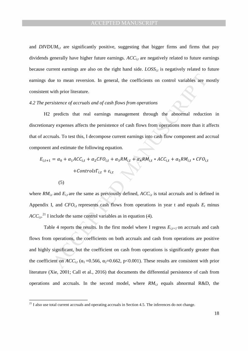
4.2 The persistence of accruals and of cash flows from operations
H2 predicts that real earnings management through the abnormal reduction in
discretionary expenses affects the persistence of cash flows from operations more than it affects
that of accruals. To test this, I decompose current earnings into cash flow component and accrual
component and estimate the following equation.
��,��� = �� + ��)!!�,� + ��!*+�,� + �����,� + �,���,� ∗ )!!�,� + �-���,� ∗ !*+�,�
+!"#$%"&'�,� + ��,�
(5)
where RMi,t and Ei,t are the same as previously defined, ACCi,t is total accruals and is defined in
Appendix I, and CFOi,t represents cash flows from operations in year t and equals Et minus
ACCi,t.21 I include the same control variables as in equation (4).
Table 4 reports the results. In the first model where I regress Ei,t+1 on accruals and cash
flows from operations, the coefficients on both accruals and cash from operations are positive
and highly significant, but the coefficient on cash from operations is significantly greater than
the coefficient on ACCi,t (α1 =0.566, α2=0.662, p<0.001). These results are consistent with prior
literature (Xie, 2001; Call et al., 2016) that documents the differential persistence of cash from
operations and accruals. In the second model, where RMi,t equals abnormal R&D, the
21 I also use total current accruals and operating accruals in Section 4.5. The inferences do not change.

MANUSCRIP
T
ACCEPTED
ACCEPTED MANUSCRIPT
19
coefficients on the interaction terms RMi,t*ACCi,t (α4) and RMi,t*CFOi,t (α5) are all negative, but
α4 is insignificant and α5 is significant and negative. Consistent with H2, the results suggest that
real earnings management through a cut in R&D significantly and negatively affects the
persistence of cash flows from operations but not accruals, implying that the impact of this type
of real earnings management on earnings persistence is largely through its negative effect on
cash from operations rather than its impact on accruals. The main effects of the accruals and cash
flows from operations remain unchanged compared with the basic model (1). Turning to the
models of other types of discretionary expenses, the results of real earnings management through
a reduction in advertising expenses (the RM_ADVi,t model) and total discretionary expenses (the
RM_TDISXi,t model) are qualitatively similar to the results of the RM_R&Di,t model and are all
consistent with H2. In model (4) of Table 4, where RM equals real earnings management
measures achieved by cutting SG&A (RM_SGAi,t), the coefficients on the interaction term
RMi,t*ACCi,t and RMi,t*CFOi,t are both significantly negative, suggesting that real earnings
management through SG&A affects both accruals and cash flows from operations. However, the
coefficient on RMi,t*ACCi,t (α4 = -0.097, t= -4.069) is smaller in the absolute magnitude than the
coefficient on RMi,t*CFOi,t (α5 = -0.227, t= -16.153). The F-test comparing these two coefficients
suggests that α5 is more negative than α4, meaning that although reducing SG&A affects the
persistence of both accruals and cash from operations, it affects cash flows from operations to a
greater extent than it affects accruals. In sum, the results in Table 4 are consistent with H2,
suggesting that the negative effect of the abnormal reduction in discretionary expenses on
earnings persistence is largely through its negative impact on the persistence of cash flows from
operations rather than through its impact on accruals.
4.3 The informativeness of current earnings

MANUSCRIP
T
ACCEPTED
ACCEPTED MANUSCRIPT
20
H3 predicts that real earnings management through the abnormal reduction in
discretionary expenses weakens the association between current earnings and future cash flows.
To test this hypothesis, I estimate equation (6).
+).!*�,��� = �� + ����,� + �����,� + �����,� ∗ ��,� + !"#$%"&'Г�,� + ��,�
(6)
where OANCFi,t represents cash flows from operations directly taken from the Statement of Cash
Flows scaled by average assets.22 Other variables are as defined in the previous models.
Table 5 reports the results. In all models, the coefficients on Ei,t are positive and highly
significant, consistent with prior literature (Atwood et al., 2010) and suggest that future cash
flows are positively associated with current earnings. When adding the RMi,t variables, the
coefficients on all the interaction terms RMi,t*Ei,t are significantly negative. Specifically, the
coefficients on RMi,t*Ei,t for the models of RM_R&Di,t, RM_ADVi,t, RM_SGAi,t, and RM_TDISCi,t
are -0.384 (t = -7.451), -0.549 (t = -3.887), -0.198 (t = -17.083), -0.347 (t = -13.812), respectively,
suggesting that current earnings are less informative about future cash flows when firms
abnormally reduce R&D, advertising, SG&A and total discretionary expenditures.
Overall, the results indicate that real earnings management through the abnormal
reduction in discretionary expenses weakens the association between current earnings and future
cash flows. The results are consistent with the notion that real earnings management is
detrimental rather than is an optimal choice for firms.
4.4 Real earnings management effect in the pre- and post- Sarbanes-Oxley periods
H4a (H4b) predicts that the effect of real earnings management on earnings persistence
(informativeness about future cash flows) is stronger in the post-SOX period. I test these
22 Here, I use cash flows from operations directly taken from the Statement of Cash Flows to ensure the measure of cash flows from operations is free of estimation errors. In robust tests, I also use cash flows from operations measures derived from the difference between earnings and accruals, and the results are qualitatively identical.

MANUSCRIP
T
ACCEPTED
ACCEPTED MANUSCRIPT
21
hypotheses by augmenting a dummy variable SOXi,t equal to 1 for the period of 2002 and beyond,
and 0 for the period before the year of 2002, and an interaction term of RMi,t*Ei,t *SOXi,t to
equation (4) and (6).
��,��� = �� + ����,� + �����,� + �����,� ∗ ��,� + �,/+0�,� + �-���,� ∗ ��,� ∗ /+0�,�
+!"#$%"&'�,� + ��,� (7a)
+).!*�,��� = �� + ����,� + �����,� + �����,� ∗ ��,� + �,/+0�,�+�-���,� ∗ ��,� ∗ /+0�,�
+!"#$%"&'�,� + ��,� (7b)
Table 6 Panel A reports the results of equation (7a). Again, the coefficients on Ei,t are
significantly positive in all model specifications. The variable of interest is the coefficients (α5)
on the three-way interaction term RMi,t*Ei,t *SOXi,t. In all the models except for the RM_ADVi,t
model, the coefficients are significantly negative, suggesting that the effect of real earnings
management through the abnormal reduction in R&D, SG&A, and total discretionary expenses
on earnings persistence is more profound in the post-SOX period. The results are generally
consistent with H4a. The coefficient on the three-way interaction term is negative but
insignificant in the RM_ADVi,t model, suggesting that an abnormal reduction in advertising
expenses does not seem to affect the earnings persistence differently in the pre- and post-SOX
periods. However, the F-test suggests that the sum of coefficients of RMi,t*Ei,t and the
coefficients on the three-way interaction terms (α3 + α5) in the RM_ADVi,t model is significantly
negative (p<0.05), consistent with my main results.
Table 6 Panel B reports the results of equation (7b). Similar to Table 6 Panel A, the
coefficients on the three-way interaction term RMi,t*Ei,t*SOXi,t are significantly negative in the
RM_R&Di,t, RM_SGAi,t, and RM_TDISXi,t models, suggesting that real earnings management
through the abnormal reduction in R&D, SG&A, and total discretionary expenses weakens the

MANUSCRIP
T
ACCEPTED
ACCEPTED MANUSCRIPT
22
association between current earnings and future cash flows after the passage of SOX. Again, the
coefficients on the three-way interaction term in the RM_ADVi,t model are negative but
insignificant, indicating that a reduction in advertising expenses does not seem to affect the
informativeness of current earnings about future cash flows differently before and after the
passage of SOX. Again, the F-test suggests that the sum of α3 and α5 in the RM_ADVi,t model is
significantly negative (p<0.05), consistent with my main results.
In sum, the results suggests that in the post-SOX periods, the effect of real earnings
management through R&D, SG&A, and total discretionary expenses reduces current earnings
persistence and its informativeness about future cash flows to a greater extent.
4.5 Additional analysis and sensitivity tests
In this section, I conduct series of additional analysis and sensitivity tests to further
validate my findings.
4.5.1 The case of meeting or just beating earnings targets
Prior studies find persuasive evidence that earnings are likely managed when firms just
meet or beat earnings target (Dechow et al., 2003; Beaver et al., 2003). Firms are also likely to
use real earnings management to meet or just beat earnings benchmarks. If meeting or just
beating earnings benchmarks is more likely to be associated with managers’ opportunistic
behavior (e.g., to increase managers’ compensation), the effect of real earnings management on
earnings quality is likely to be more pronounced when firms use real earnings management to
meet or just beat earnings benchmarks. However, because firms meet or just beat earnings targets
for different reasons, how meeting or beating earnings benchmarks affects the negative effect of
real earnings management on earnings quality is not entirely clear. To investigate this issue,
following Gunny (2010), I define a variable MBTi,t equal to one if firms meet the zero earnings

MANUSCRIP
T
ACCEPTED
ACCEPTED MANUSCRIPT
23
target or last year’s target, or if current earnings are greater than zero earnings or last year’s
earnings by 0.01. I then estimate equation (8a) and (8b) to test whether the negative effect of real
earnings management through the abnormal reduction in discretionary expenditures is stronger
for firms that meet or just beat earnings targets.
��,��� = �� + ����,� + �����,� + �����,� ∗ ��,� + �,�12�,� + �-���,� ∗ ��,� ∗ �12�,�
+!"#$%"&'�,� + ��,� (8a)
+).!*�,��� = �� + ����,� + �����,� + �����,� ∗ ��,� + �,�12�,�+�-���,� ∗ ��,� ∗ �12�,�
+!"#$%"&'�,� + ��,� (8b)
The variable of interest is the interaction term of RMi,t*Ei,t *MBTi,t. A negative coefficient
indicates that firms that engage in real earnings management to meet or just beat earnings targets
have even lower earnings persistence. Table 7 reports the results.23 In both Panel A and Panel B,
the coefficients on RMi,t*Ei,t*MBTi,t are significantly negative for the models of RM_R&Di,t and
RM_TDISXi,t, suggesting that the negative effect of the abnormal reduction in R&D and total
discretionary expenses on earnings persistence and current earnings’ ability to predict future cash
flows are worsened when firms meet or just beat earnings targets. In the tests of RM_SGAi,t, the
coefficients on the three-way interaction term are significantly negative in the earnings
persistence tests (Table 7 Panel A) but insignificant in the future cash flow informativeness tests
(Table 7 Panel B). Further, the tests of RM_ADVi,t show insignificant coefficients on both tests.
In sum, I find evidence that the negative effect of abnormal reductions in R&D and total
discretionary expenses is stronger for firms that meet or just beat earnings targets but mixed
evidence on the effect of abnormal reductions in other types of discretionary expenses.
4.5.2 Controling for accrual earnings management
23 The significant negative coefficient on MBTi,t in the basic model of Table 7 Panel A probably is due to the fact that MBTi,t is associated with earnings management and that current period earnings management has a negative effect on future earnings.

MANUSCRIP
T
ACCEPTED
ACCEPTED MANUSCRIPT
24
The extant literature generally indicates that large accruals are less persistent (Sloan,
1996; Richardson et al., 2005). Xie (2001) finds that discretionary accruals have a significantly
positive but lower persistence coefficient than normal accruals and cash flows from operations.
Blaylock et al. (2012) documents that firms with large positive book-tax differences consisting of
large positive accruals have less persistent earnings. Real earnings management affects both
accruals and cash flows, and it is possible that the effect of the abnormal reduction in
discretionary expenses on earnings persistence and its informativeness about future cash flows
are driven by the effect of accrual earnings management (proxied by large accruals). To mitigate
this concern, I control for the effect of accrual earnings management and rerun my tests. I proxy
accrual earnings management by top quintile of the absolute values of discretionary accruals,
defined as the residuals of the modified Jones model.24 I then estimate equation (9a) and (9b) to
test whether real earnings management has incremental effects on earnings quality.25
��,��� = �� + ����,� + �����,� + �����,� ∗ ��,� + �,3)�,� + �- ∗ �� ∗ 3)�,�
+!"#$%"&'�,� + ��,� (9a)
+).!*�,��� = �� + ����,� + �����,� + �����,� ∗ ��,� + �,3)�,�+�-��,� ∗ 3)�,�
+!"#$%"&'�,� + ��,� (9b)
where DAi,t equals one for firm-year observations with the absolute values of modified Jones
model discretionary accruals in the top quintile of all firm-years in the sample. Table 8 reports
the results. The coefficients on the interaction terms of RMi,t*Ei,t are significantly negative for all
RM models, even after controlling for the effect of accrual earnings management on earnings
persistence. The results suggest that real earnings management affects earnings persistence and
24 To identify the strongest setting of accrual management, I use the top quintile of the absolute values of discretionary accruals. Untabulated results are generally similar when I proxy accruals management by the level of discretionary accruals. 25 In untabulated tests, I include all the control variables used in my main analysis except for ACCi,t. My inferences do not change.

MANUSCRIP
T
ACCEPTED
ACCEPTED MANUSCRIPT
25
its association with future cash flows beyond the effect of accrual earnings management.
Consistent with prior literature (Blaylock et al., 2012; Richardson et al., 2005) that larger
accruals are less persistent, the coefficients on DAi,t and DAi,t*Ei,t are also significantly negative.
In sum, the results of Table 8 indicate that the effects of real earnings management on earnings
persistence and its informativeness about future cash flows are incremental to the effects of
accruals and accruals earnings management.
4.5.3 Alternative real earnings management measures
In my main tests, I follow prior literature to measure the extent of real earnings
management through the abnormal reduction in discretionary expenses. One difficulty in
measuring the abnormal level is that the optimal level of discretionary expenses is subject to the
specification of the model. To test whether my results are robust to an alternative measure of real
earnings management, I use a different R&D model to estimate the normal level of R&D
expenditures. Ewert and Wagenhofer (2005) develop an analytical model and demonstrate that
firms with less accrual flexibility are more likely to choose real earnings management. Using the
R&D model developed by Berger (1993) and the theory of Ewert and Wagenhofer (2005), I
identify firms suspected of real earnings management by focusing on the firms with both
abnormally low R&D expenditures and low accounting flexibility. 26 The suspect real earnings
maangement sample is 5% (3,688 firm-years) of the sample used for this test (total 81,652 firm
years). I define a new dummy variable DRM_AR&Di,t equal to 1 for firm-years in the suspect
real earnings management sample and 0 otherwise.
I rerun equation (4) and (6) using the alternative measure of real earnings management.
Table 9 reports the results. Consistent with H1 and H3, the interaction terms DRM_AR&Di,t*Ei,t
26 See Appendix I for an alternative definition of real earnings management.

MANUSCRIP
T
ACCEPTED
ACCEPTED MANUSCRIPT
26
are significantly negative in both the earnings persistence model and future cash flow model.
Therefore, my results are robust to the alternative measure of real earnings management.
4.5.4 Other sensitivity tests
To examine whether my results are robust to different model modifications, I test my
hypotheses by using alternative earnings persistence models. In untabulated tests, I use
persistence models developed by Li (2008), Li and Mohanram (2014), and So (2013) that include
a different set of control variables, and my results are robust to these alternative model
specifications. 27
In my main tests, I classify industries based on Fama-French 48 classification. As a
robustness check, I use two-digit SIC code to define industries. Untabulated results are
qualitatively similar. To check whether firms abnormally reduce discretionary expenses
consecutively, I calculate serial correlation of the firms’ real earnings management level in my
sample. Untabulated results show positive but small serial correlations for my measures of real
earnings management, suggesting that the abnormal reduction in discretionary expenses may last
more than one year. However, my findings suggest that real earnings management through the
abnormal reduction in discretionary expenses, on average, decreases earnings persistence.
To examine whether my results are sensitive to the definition of earnings, cash flows
from operations, and accruals, I re-examine all my hypotheses using other definitions of these
variables. I follow Atwood et al. (2010) to examine pre-tax income persistence and the
association between earnings and cash flows from operations where cash from operations is
defined as pre-tax income minus accruals. I also use current accruals and operating accruals (Call
27 The Li and Mohanram (2014) model is essentially a model to control for negative earnings. The model of So (2013) is also used by Call et al. (2016). When using the Li (2008) model, due to a significant reduction in sample size, the coefficient on RMi,t *Ei,t in the RM_ADVi,t model is negative but insignificant. However, in all other specifications, I find consistent results with my main analysis.

MANUSCRIP
T
ACCEPTED
ACCEPTED MANUSCRIPT
27
et al., 2016) instead of total accruals to test H2. Untabulated results suggest that my inferences
do not change.
In my main tests, I use different samples for the tests of each individual type of
discretionary expenses to maximize my sample size.28 In sensitivity tests, I construct a common
sample that have non-missing data for all types of discretionary expenses to re-run all my tests.
Restricting observations to have all the available data for R&D, advertising, and SG&A expenses
significantly reduces my sample to 34,407 firm-years. The purpose of these tests is to check
whether my results are sensitive to different samples. All my results (untabulated) remain
qualitatively similar except for one case.29
5. Conclusions
In this paper, I examine whether real earnings management affects two important aspects
of earnings quality: the persistence and informativeness of current earnings. I focus my study of
real earnings management on the abnormal reduction in discretionary expenses and use the
models developed by Roychowdhury (2006) to estimate the abnormal level of discretionary
expenses. Managers can cut discretionary expenditures to opportunistically increase current
period earnings or to signal their private information about positive future profitability. Because
real earnings management through the abnormal reduction in discretionary expenses is usually
achieved at the cost of forgoing positive NPV projects, such type of earnings management is
more likely to be detrimental to future performance. Therefore, real earnings management
28 For example, in testing the abnormal reduction in R&D expenditures, I set missing R&Di,t to be zero but do not set missing SGAi,t and ADVi,t to be zero. When testing the advertising expenses, I set missing ADVi,t to be zero but do not set missing R&Di,t and SGAi,t to be zero. Therefore, my samples for each specific type of real earnings management are slightly different. 29 In testing H2 for opportunistic R&D reduction, the coefficients on RM_R&Di,t*CFOi,t is not greater in magnitude than RM_R&Di,t*ACCi,t, although both are significantly negative.

MANUSCRIP
T
ACCEPTED
ACCEPTED MANUSCRIPT
28
through the abnormal reduction in discretionary expenses is more likely to decrease earnings
persistence.
Examining a sample over a period of 41 years, I find that earnings persistence decreases in
all my measures of real earnings management. The results are consistent with prior research that
documents the negative association between real earnings management and firms’ future
performance. In testing whether such an effect on earnings persistence is through cash flows or
accruals, I find that real earnings management by abnormal reductions in all types of
discretionary expenditures affects cash from operations more than it affects accruals.
Furthermore, my results suggest that the less persistent earnings as a result of real earnings
management are less informative about future cash flows.
This study contributes to the literature on examining earnings quality under a certain type
of earnings management. Prior study documents a trend that managers increase the use of real
operational activities to manage earnings after the passage of SOX. The results of my study
indicate that real earnings management negatively affects earnings quality, especially the quality
of cash flows. Extant research examining earnings quality largely focuses on accrual quality,
implicitly assuming cash flows are free of manipulation. My findings suggest that future
researchers should consider both accrual and real earnings management when conducting
earnings quality research.

MANUSCRIP
T
ACCEPTED
ACCEPTED MANUSCRIPT
29
References
Atwood, T. J., M. S. Drake, and L. A. Myers, 2010. Book-tax conformity, earnings persistence and the association between earnings and future cash flows. Journal of Accounting and Economics 50: 111-125. Baber, W., P. Fairfield, and J. Haggard, 1991. The effect of concern about reported income on discretionary spending decisions. The Accounting Review 66: 818-829. Barton, J. and P. Simko, 2002. The balance sheet as an earnings management constraint. The Accounting Review 77: 1-27. Beaver, W., M. McNichols, and K. Nelson, 2003. Management of the loss reserve accrual and the distribution of earnings in the property-casualty insurance industry. Journal of accounting and Economics 35: 347-376. Blaylock, B., T. Shevlin., R. J. Wilson, 2012. Tax avoidance, large positive temporary book-tax differences, and earnings persistence. The Accounting Review 87(1):91-120. Bushee, B., 1998. The influence of institutional investors on myopic R&D investment behavior. The Accounting Review 73: 305-33. Call, A. C., M. Hewitt, T. Shevlin, and T. L. Yohn, 2016. Firm-specific estimates of differential persistence and their incremental usefulness for forecasting and valuation. The Accounting Review 91(3): 811-833. Cohen, D. A., A. Dey, and T. Z. Lys, 2008. Real and accrued-based earnings management in the pre- and post-Sarbanes-Oxley periods. The Accounting Review 83 (3):757-787. Collins, D. W. and S. P. Kothari. 1989. An analysis of intertemporal and cross-sectional determinants of earnings response coefficients. Journal of Accounting and Economics 11: 143-181. Cheng, Q., J. Lee, and T. Shevlin, 2016. Internal governance and real earnings management. The Accounting Review 91 (4):1051-1085. Dechow, P. M. and I. D. Dichev, 2002. The quality of accruals and earnings: the role of accrual estimation errors. The Accounting Review 77 (Supplement): 35-42. Dechow, P. M., W. Ge, and C. Schrand. 2010. Understanding earnings quality: A review of the proxies, their determinants and their consequences. Journal of Accounting and Economics Dechow, P. M., Richardon, S., and I. Tuna, 2003. Why are earnings kinky? An examination of the earnings management explanation. Review of Accounting Studies 8: 355-384.
MANUSCRIP
T
ACCEPTED
ACCEPTED MANUSCRIPT
30
Dechow, P. M. and R. Sloan, 1991. Executive incentives and the horizon problem: an empirical investigation. Journal of Accounting and Economics 14: 51-89. Dechow, P. M., R. Sloan, and A. Sweeney, 1995. Detecting earnings management. The Accounting Review 70:193-225. DeFond, M. L., 2010. Earnings quality research: advances, challenges and future research. Journal of Accounting and Economics 50: 402-409. Ewert, R. and A. Wagenhofer, 2005. Economic effects of tightening accounting standards to restrict earnings management. The Accounting Review 80: 1101-1124. Francis, J., R. LaFond, P. Olsson and K. Schipper, 2005. The market pricing of accruals quality. Journal of Accounting and Economics 39: 295-327. Graham, J., C. Harvey, and S. Rajpogpal, 2005. The Economic Implications of Corporate Financial Reporting. Journal of Accounting and Economics 40: 3-73. Gunny, K, 2010. The relation between earnings management using real activity and future performance: evidence from meeting earnings benchmarks. Contemporary Accounting Research 27 (3): 855-888. Hanlon, M., 2005. The persistence and pricing of earnings, accruals, and cash flows when firms have large book-tax differences. The Accounting Review 80(1): 137-166. Hayn, C., 1995. The information content of losses. Journal of Accunting & Economics 20: 125-153. Hou, K., M. A. Van Dijk, and Y. Zhang, 2012. The implied cost of capital: A new approach. Journal of Accounting and Economics 53: 504-526. Kothari, S. P., N. Mizik, and S. Roychowdhury, 2016. Managing for the moment: The role of earnings management via real activies versus accruals in SEO valuation. The Accounting Review 91(2): 559-586. Kormendi, R. and R. Lipe. 1987. Earnings Innovations, Earnings Persistence, and Stock Returns. The Journal of Business 60(3): 323-345.
Lee, L. F., 2012. Incentives to inflate reported cash from operations using classification and timing. The Accounting Review 87(1): 1-33.
Li, F., 2008. Annual report readability, current earnings, and earnings persistence. Journal of Accounting and Economics 45: 221-247. Li, K. K. and P. Mohanram, 2014. Evaluating cross-sectional forecasting models for implied cost of capital. Review of Accounting Studies 19: 1152-1185.

MANUSCRIP
T
ACCEPTED
ACCEPTED MANUSCRIPT
31
Li, V., 2016. Do False Financial Statements Distort Peer Firms' Decisions? The Accounting Review 91(1): 251-278. Mizik, N. and R. Jacobson, 2007. Myopic marketing management: evidence of the phenomenon and its long-term performance consequences in the SEO context. Marketing Science 26(3): 361-379. Perry, S. and R. Grinaker, 1994. Earnings expectations and discretionary research and development spending. Accounting Horizons 8: 43-51. Richardson, S.A., R.G. Sloan, M.T. Soliman, and I. Tuna, 2005. Accrual reliability, earnings persistence and stock prices. Journal of Accounting and Economics 39: 437-485. Roychowdhury, S., 2006. Earnings Management through real activities manipulation. Journal of Accounting and Economics 42: 335-370. Shipper, K., and L. Vincent, 2003. Earnings quality. Accounting Horizons 17: 97-110. Sloan, R., 1996. Do stock prices fully reflect information in accruals and cash flows about future earnings? The Accounting Review 71: 289-315. So, E. C., 2013. A new approach to predicting analyst forecast errors: Do investors overweight analyst forecasts? Journal of Financial Economics 108: 615-640. Subramanyam, K. R., 1996. The pricing of discretionary accruals. Journal of Accounting and Economics 22: 249-281. Xie, H., 2001. The mispricing of abnormal accruals. The Accounting Review 76(3): 357-373. Zang, A.Y., 2012. Evidence on the tradeoff between real manipulation and accrual-based earnings management. The Accounting Review 87 (2): 675-703.
MANUSCRIP
T
ACCEPTED
ACCEPTED MANUSCRIPT
32
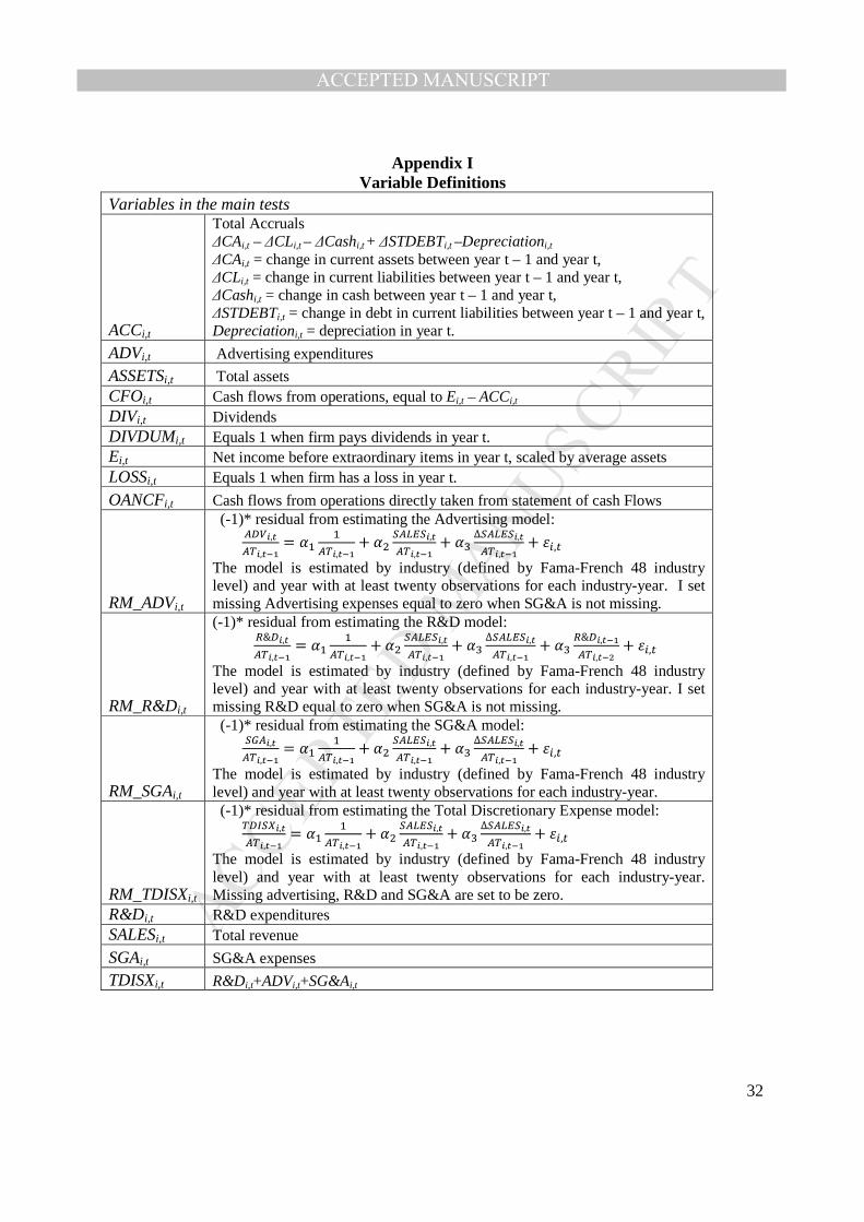
Appendix I Variable Definitions
Variables in the main tests
ACCi,t
Total Accruals ∆CAi,t – ∆CLi,t – ∆Cashi,t + ∆STDEBTi,t –Depreciationi,t ∆CAi,t = change in current assets between year t – 1 and year t, ∆CLi,t = change in current liabilities between year t – 1 and year t, ∆Cashi,t = change in cash between year t – 1 and year t, ∆STDEBTi,t = change in debt in current liabilities between year t – 1 and year t, Depreciationi,t = depreciation in year t.
ADVi,t Advertising expenditures
ASSETSi,t Total assets CFOi,t Cash flows from operations, equal to Ei,t – ACCi,t
DIVi,t Dividends DIVDUMi,t Equals 1 when firm pays dividends in year t. Ei,t Net income before extraordinary items in year t, scaled by average assets LOSSi,t Equals 1 when firm has a loss in year t.
OANCFi,t Cash flows from operations directly taken from statement of cash Flows
RM_ADVi,t
(-1)* residual from estimating the Advertising model: ��4�,�
��,���= ��
���,���
+ �������,���,���
+ ��∆�����,���,���
+ ��,�
The model is estimated by industry (defined by Fama-French 48 industry level) and year with at least twenty observations for each industry-year. I set missing Advertising expenses equal to zero when SG&A is not missing.
RM_R&Di,t
(-1)* residual from estimating the R&D model:
�&��,�
��,���= ��
���,���
+ �������,���,���
+ ��∆�����,���,���
+ ���&��,���
��,���+ ��,�
The model is estimated by industry (defined by Fama-French 48 industry level) and year with at least twenty observations for each industry-year. I set missing R&D equal to zero when SG&A is not missing.
RM_SGAi,t
(-1)* residual from estimating the SG&A model: �5��,�
��,���= ��
���,���
+ �������,���,���
+ ��∆�����,���,���
+ ��,�
The model is estimated by industry (defined by Fama-French 48 industry level) and year with at least twenty observations for each industry-year.
RM_TDISXi,t
(-1)* residual from estimating the Total Discretionary Expense model: �����,�
��,���= ��
���,���
+ �������,���,���
+ ��∆�����,���,���
+ ��,�
The model is estimated by industry (defined by Fama-French 48 industry level) and year with at least twenty observations for each industry-year. Missing advertising, R&D and SG&A are set to be zero.
R&Di,t R&D expenditures SALESi,t Total revenue
SGAi,t SG&A expenses
TDISXi,t R&Di,t+ADVi,t+SG&Ai,t

MANUSCRIP
T
ACCEPTED
ACCEPTED MANUSCRIPT
33
Appendix I (Continued)
Variables in the additional tests
DAi,t
Equals 1 for firms with discretionary accruals in the top quintile of absolute residuals estimated from the Modified Jones model (Dechow et al., 1995):
)!!�,� = � + 6�7∆�89�,� − ∆�8;�,�< + 6�==��,� + ��,�
where Revi,t is total sales; Reci,t is accounts receivable, and PPEi,t is property, plant, and equipment all scaled by average total assets; and 0 otherwise.
DRM_AR&Di,t
Equals 1 for firm-year suspected of engaging in real earnings management, and 0 otherwise. Suspected real earnings management firm-years are those in the lowest abnormal R&D expense quintile and the highest NOA quintile. The abnormal R&D is (-1)* residuals from the alternative R&D model, estimated cross-sectionally for each Fama-French 48 industry group each year.
�&3�,� = �� + 6��&3�,�>� + 6�?.2�,� + 6�@�,� + 6,!0�,� + 6-�A� + ��,� where INTi,t is Internal fund, equal to (Ei,t + R&Di,t + Depreciationi,t)/SALESi,t; Qi,t is Tobin’s Q deflated by lagged total assets and calculated as (market value of equity + book value of preferred stock + short-term debt + long-term debt) / total assets; CXi,t is capital expenditures scaled by lagged total assets; MVi,t is log of market value of equity; NOAi,t-1 is net operating assets in year t – 1 as defined in Barton and Simko (2002), and calculated as (�@C?2D�,�>� − !)/E�,�>� −�F2/�!�,�>� +3�12�,�>�)//)I�/�,�>�, where EQUITYi,t –1 is the lagged shareholder’s equity; CASHi,t –1 is lagged cash; MKESECi,t –1 is lagged marketable security; DEBTi,t –1 is lagged total debt.30
MBTi,t
Equals 1 if firms just meet the zero earnings targets or last years’ earnings or if current earnings are greater than zero earnings or last years’ earnings scaled by total assets by 0.01.
SOXi,t Equals 1 for the year of 2002 and beyond, and 0 otherwise.
30 This procedure is stricter and less commonly used in prior literature. Therefore, I do not use this approach in my main tests.

MANUSCRIP
T
ACCEPTED
ACCEPTED MANUSCRIPT
34
Table 1 Derivation of Sample: 1975 – 2016
Firm-years with positive sales, cost of goods for sale, inventory, assets greater than 1 million 214,170
Firm-years with non-missing earnings 176,460
Firm-years with sufficient data to calculate accruals and CFO 171,280 Final sample with sufficient data to calculate total discretionary expenses 161,941
Samples used to estimate different types of real earnings management are different in size to maximize the sample size for each test.

MANUSCRIP
T
ACCEPTED
ACCEPTED MANUSCRIPT
35
Table 2 Descriptive Statistics
Variable N Mean sddev Min Q1 Median Q3 Max ASSETSi,t 176460 1101.7 3555 1.39 18.62 87.28 470.58 26144 Ei,t 176460 -0.013 0.181 -0.744 -0.038 0.034 0.080 0.309 OANCFi,t 125391 0.032 0.178 -0.722 -0.014 0.066 0.129 0.380 LOSSi,t 176460 0.330 0.470 0.000 0.000 0.000 1.000 1.000 RM_R&Di,t 148504 -0.004 0.056 -0.309 -0.002 0.000 0.005 0.190 RM_ADVi,t 160943 0.000 0.037 -0.195 -0.003 0.003 0.010 0.101 RM_SGAi,t 156943 -0.025 0.283 -1.082 -0.133 -0.009 0.088 1.002 RM_TDISXi,t 166336 -0.007 0.085 -0.220 -0.029 0.002 0.025 0.284 ASSETSi,t is Total Assets; Ei,t is net income before extraordinary items; OANCFi,t is cash flows from operations from Statement of Cash flows; LOSSi,t equals 1 if firms have a loss in year t and zero otherwise; RM_R&Di,t is the abnormal level of R&D expenditures; RM_ADVi,t is the abnormal level of advertising expenditures; RM_SGAi,t is the abnormal level of SG&A expenditures; and RM_TDISXi,t is the abnormal level of total discretionary expenditures. All variables are defined in Appendix I, and, except for the dummy variables, are scaled by average assets and winsorized at 1 and 99 percent level.

MANUSCRIP
T
ACCEPTED
ACCEPTED MANUSCRIPT
36
Table 3 Association between Earnings Persistence and Real Earnings Management
Model:��,��� = �� + ����,� + �����,� + �����,� ∗ ��,� + !"#$%"&'Г�,� + ��,� (1) (2) (3) (4) (5) VARIABLES Basic RM_R&Di,t RM_ADV i,t RM_SGAi,t RM_TDISXi,t
Ei,t 0.708*** 0.702*** 0.693*** 0.645*** 0.665*** (114.622) (98.567) (103.909) (86.773) (95.086) RMi,t 0.070*** 0.075*** 0.021*** 0.080*** (4.653) (5.203) (11.003) (13.154) RMi,t * Ei,t -0.119** -0.604*** -0.136*** -0.188*** (-2.051) (-4.090) (-10.681) (-7.131) Log(ASSETS)i,t 0.010*** 0.010*** 0.010*** 0.009*** 0.011*** (32.707) (30.286) (31.092) (29.787) (33.307) DIVi,t 0.292*** 0.305*** 0.270*** 0.282*** 0.307*** (15.210) (14.464) (13.857) (13.754) (15.590) DIVDUMi,t 0.007*** 0.006*** 0.007*** 0.007*** 0.006*** (7.940) (6.831) (8.177) (8.222) (6.482) LOSSi,t -0.014*** -0.014*** -0.015*** -0.020*** -0.018*** (-10.253) (-8.987) (-10.564) (-13.372) (-12.295) ACCi,t -0.126*** -0.126*** -0.122*** -0.115*** -0.121*** (-23.654) (-21.126) (-22.694) (-21.237) (-22.214) Constant -0.026*** -0.029*** -0.027*** -0.026*** -0.028*** (-5.398) (-4.191) (-4.857) (-4.328) (-4.967) Observations 171,280 144,904 156,809 153,218 161,941 Adjusted R-squared 0.493 0.489 0.464 0.462 0.495 IndDummies Yes Yes Yes Yes Yes YearDummies Yes Yes Yes Yes Yes SE ClusteredBy Firm Firm Firm Firm Firm Model is estimated by running a pooled regression on all firm-years 1975-2016. Ei,t is net income before extraordinary items. RMi,t equals RM_R&Di,t, RM_ADVi,t, RM_SGAi,t, and RM_TDISXi,t in model (2), (3), (4), and (5), respectively. RM_R&Di,t is the abnormal level of R&D expenditures; RM_ADVi,t is the abnormal level of advertising expenditures; RM_SGAi,t is the abnormal level of SG&A expenditures; and RM_TDISXi,t is the abnormal level of total discretionary expenditures. Log(ASSETS)i,t is the nature log of total assets; DIVi,t is dividends, DIVDUMi,t equals 1 when firm i pays dividends in year t, and 0 otherwise; LOSSi,t equals 1 when firm i has a loss in year t., and 0 other wise; ACCi,t is total accruals. All variables are defined in Appendix I, and, except for the dummy variables, are scaled by average assets and winsorized at 1 and 99 percent level. Standard errors are clustered by firm. Robust t-statistics in parentheses. *** p<0.01, ** p<0.05, * p<0.1, based on two-tailed tests.

MANUSCRIP
T
ACCEPTED
ACCEPTED MANUSCRIPT
37
Table 4 The Effect of Real Earnings Management on Accruals and Cash Flows from Operations
Model: ��,��� = �� + ��)!!�,� + ��!*+�,� + �����,� + �,���,� ∗ )!!�,� + �-���,� ∗ !*+�,� +!"#$%"&'Г�,� + ��,� (1) (2) (3) (4) (5) VARIABLES Basic RM_R&Di,t RM_ADV i,t RM_SGAi,t RM_TDISXi,t ACCi,t 0.566*** 0.557*** 0.554*** 0.502*** 0.520*** (70.560) (62.052) (66.153) (57.245) (61.137) CFOi,t 0.662*** 0.654*** 0.647*** 0.582*** 0.608*** (105.005) (90.344) (94.734) (78.845) (85.852) RMi,t 0.075*** 0.096*** 0.031*** 0.081*** (5.078) (5.386) (14.127) (13.124) RMi,t*ACCi,t -0.069 -0.306 -0.097*** 0.025 (-0.414) (-1.348) (-4.069) (0.388) RMi,t*CFOi,t -0.269*** -0.803*** -0.227*** -0.352*** (-4.030) (-5.325) (-16.153) (-12.130) Log(ASSETS)i,t 0.011*** 0.011*** 0.011*** 0.010*** 0.012*** (33.678) (31.128) (31.563) (30.259) (33.849) DIVi,t 0.360*** 0.376*** 0.334*** 0.343*** 0.373*** (16.992) (16.207) (15.562) (15.283) (17.291) DIVDUMi,t 0.004*** 0.004*** 0.004*** 0.005*** 0.003*** (3.813) (3.543) (4.444) (5.184) (3.299) LOSSi,t -0.030*** -0.030*** -0.032*** -0.037*** -0.035*** (-21.129) (-18.990) (-21.215) (-24.521) (-23.299) Constant -0.044*** -0.049*** -0.045*** -0.041*** -0.044*** (-7.630) (-6.189) (-7.021) (-6.075) (-6.916) Observations 171,280 144,904 156,809 153,218 161,941 Adjusted R-squared 0.479 0.476 0.448 0.450 0.483 IndDummies Yes Yes Yes Yes Yes YearDummies Yes Yes Yes Yes Yes SE ClusteredBy Firm Firm Firm Firm Firm Model is estimated by running a pooled regression on all firm-years 1975-2016. Ei,t is net income before extraordinary items. RMi,t equals RM_R&Di,t, RM_ADVi,t, RM_SGAi,t, and RM_TDISXi,t in model (2), (3), (4), and (5), respectively. RM_R&Di,t is the abnormal level of R&D expenditures; RM_ADVi,t is the abnormal level of advertising expenditures; RM_SGAi,t is the abnormal level of SG&A expenditures; and RM_TDISXi,t is the abnormal level of total discretionary expenditures. Log(ASSETS)i,t is the nature log of total assets; DIVi,t is dividends, DIVDUMi,t equals 1 when firm i pays dividends in year t, and 0 otherwise; LOSSi,t equals 1 when firm i has a loss in year t., and 0 other wise; ACCi,t is total accruals. CFO is cash flows from operations. All variables are defined in Appendix I, and, except for the dummy variables, are scaled by average assets and winsorized at 1 and 99 percent level. Standard errors are clustered by firm. Robust t-statistics in parentheses. *** p<0.01, ** p<0.05, * p<0.1, based on two-tailed tests.

MANUSCRIP
T
ACCEPTED
ACCEPTED MANUSCRIPT
38
Table 5 The Effect of Real Earnings Management on the Association between Current Earnings
and Future Cash Flows
Model: +).!*�,��� = �� + ����,� + �����,� + �����,� ∗ ��,� + !"#$%"&'Г�,� + ��,� (1) (2) (3) (4) (5) VARIABLES Basic RM_R&Di,t RM_ADVi,t RM_SGAi,t RM_TDISXi,t Ei,t 0.540*** 0.517*** 0.520*** 0.453*** 0.474*** (89.644) (77.566) (81.608) (67.203) (72.925) RMi,t 0.077*** 0.052*** 0.017*** 0.073*** (5.568) (3.351) (8.327) (10.666) RMi,t * Ei,t -0.384*** -0.549*** -0.198*** -0.347*** (-7.451) (-3.887) (-17.083) (-13.812) Log(ASSETS)i,t 0.011*** 0.011*** 0.011*** 0.010*** 0.012*** (29.658) (28.133) (29.775) (28.566) (31.265) DIVi,t 0.255*** 0.380*** 0.242*** 0.276*** 0.303*** (5.242) (7.177) (4.941) (5.398) (6.050) DIVDUMi,t 0.009*** 0.007*** 0.008*** 0.009*** 0.008*** (7.066) (5.230) (6.881) (6.892) (6.016) LOSSi,t 0.004*** 0.002 0.003** -0.004*** -0.003** (2.763) (1.537) (2.032) (-3.010) (-2.231) ACCi,t -0.208*** -0.194*** -0.205*** -0.193*** -0.196*** (-34.030) (-29.178) (-32.873) (-30.796) (-31.295) Constant -0.028*** -0.018 -0.026** -0.020* -0.028*** (-2.787) (-1.568) (-2.455) (-1.892) (-2.629) Observations 121,736 106,434 111,073 108,928 115,563 Adjusted R-squared 0.474 0.473 0.430 0.432 0.482 IndDummies Yes Yes Yes Yes Yes YearDummies Yes Yes Yes Yes Yes SE ClusteredBy Firm Firm Firm Firm Firm Model is estimated by running a pooled regression on all firm-years 1988-2016. OANCF is Cash flows from operations directly taken from Statement of Cash Flows; Ei,t is net income before extraordinary items. RMi,t equals RM_R&Di,t, RM_ADVi,t, RM_SGAi,t, and RM_TDISXi,t in model (2), (3), (4), and (5), respectively. RM_R&Di,t is the abnormal level of R&D expenditures; RM_ADVi,t is the abnormal level of advertising expenditures; RM_SGAi,t is the abnormal level of SG&A expenditures; and RM_TDISXi,t is the abnormal level of total discretionary expenditures. Log(ASSETS)i,t is the nature log of total assets; DIVi,t is dividends, DIVDUMi,t equals 1 when firm i pays dividends in year t, and 0 otherwise; LOSSi,t equals 1 when firm i has a loss in year t., and 0 other wise; ACCi,t is total accruals. All variables are defined in Appendix I, and, except for the dummy variables, are scaled by average assets and winsorized at 1 and 99 percent level. Standard errors are clustered by firm. Robust t-statistics in parentheses. *** p<0.01, ** p<0.05, * p<0.1, based on two-tailed tests.

MANUSCRIP
T
ACCEPTED
ACCEPTED MANUSCRIPT
39
Table 6 The Effect of Real Earnings Management on Earnings Quality Pre- and Post- SOX
Panel A:��,��� = �� + ����,� + �����,� + �����,� ∗ ��,� + �,/+0�,� + �-���,� ∗ ��,� ∗/+0�,� + !"#$%"&'Г�,� + ��,� (1) (2) (3) (4) (5) VARIABLES Basic RM_R&Di,t RM_ADVi,t RM_SGAi,t RM_TDISXi,t Ei,t 0.735*** 0.732*** 0.722*** 0.676*** 0.697*** (118.610) (101.337) (107.728) (88.390) (97.170) RMi,t 0.035** 0.059*** 0.020*** 0.057*** (2.277) (4.163) (10.286) (9.390) RMi,t * Ei,t -0.042 -0.747*** -0.089*** -0.139*** (-0.577) (-4.565) (-5.397) (-4.452) SOXi,t -0.009 -0.007 -0.007 -0.008 -0.008 (-1.038) (-0.796) (-0.816) (-0.823) (-0.910) RMi,t * Ei,t * SOXi,t -0.200** 0.477 -0.095*** -0.123*** (-2.193) (1.458) (-4.085) (-3.105) Log(ASSETS)i,t -0.046*** -0.036*** -0.055*** -0.044*** -0.033*** (-12.058) (-7.527) (-13.751) (-10.310) (-7.927) DIVi,t -0.089*** -0.086*** -0.091*** -0.078*** -0.093*** (-5.639) (-5.015) (-5.686) (-4.623) (-5.763) DIVDUMi,t 0.028*** 0.028*** 0.027*** 0.028*** 0.029*** (37.699) (34.984) (37.251) (36.792) (37.919) LOSSi,t -0.018*** -0.017*** -0.019*** -0.023*** -0.021*** (-12.663) (-10.875) (-12.913) (-15.227) (-14.255) ACCi,t -0.117*** -0.121*** -0.108*** -0.106*** -0.118*** (-20.135) (-18.745) (-18.476) (-17.946) (-19.945) Constant 0.046*** 0.033*** 0.054*** 0.042*** 0.032*** (7.516) (3.989) (7.696) (5.676) (4.531) Observations 171,280 144,904 156,809 153,218 161,941 Adjusted R-squared 0.489 0.484 0.460 0.458 0.489 IndDummies Yes Yes Yes Yes Yes YearDummies Yes Yes Yes Yes Yes SE ClusteredBy Firm Firm Firm Firm Firm Model is estimated by running a pooled regression on all firm-years 1975-2016. Ei,t is net income before extraordinary items. RMi,t equals RM_R&Di,t, RM_ADVi,t, RM_SGAi,t, and RM_TDISXi,t in model (2), (3), (4), and (5), respectively. RM_R&Di,t is the abnormal level of R&D expenditures; RM_ADVi,t is the abnormal level of advertising expenditures; RM_SGAi,t is the abnormal level of SG&A expenditures; and RM_TDISXi,t is the abnormal level of total discretionary expenditures. Log(ASSETS)i,t is the nature log of total assets; DIVi,t is dividends, DIVDUMi,t equals 1 when firm i pays dividends in year t, and 0 otherwise; LOSSi,t equals 1 when firm i has a loss in year t., and 0 other wise; ACCi,t is total accruals; SOXi,t equals 1 for period of year 2002 and beyond; 0 otherwise. All variables are defined in Appendix I, and, except for the dummy variables, are scaled by average assets and winsorized at 1 and 99 percent level. All variables except for dummy variables are scaled by average assets and winsorized at 1 and 99 percent level. Standard errors are clustered by firm. Robust t-statistics in parentheses. *** p<0.01, ** p<0.05, * p<0.1, based on two-tailed tests.

MANUSCRIP
T
ACCEPTED
ACCEPTED MANUSCRIPT
40
Table 6 (Continued)
Panel B: +).!*�,��� = �� + ����,� + �����,� + �����,� ∗ ��,� + �,/+0�,� + �-���,� ∗ ��,� ∗/+0�,� + !"#$%"&'Г�,� + ��,� (1) (2) (3) (4) (5) VARIABLES Basic RM_R&Di,t RM_ADVi,t RM_SGAi,t RM_TDISXi,t Ei,t 0.570*** 0.570*** 0.568*** 0.487*** 0.510*** (95.260) (84.997) (87.103) (71.297) (77.708) RMi,t 0.041*** 0.036** 0.016*** 0.050*** (2.901) (2.360) (7.734) (7.256) RMi,t * Ei,t -0.533*** -0.486*** -0.170*** -0.310*** (-8.570) (-3.002) (-11.397) (-10.835) SOXi,t 0.009 -0.003 0.004 0.012 0.013 (0.953) (-0.257) (0.438) (1.315) (1.370) RMi,t * Ei,t * SOXi,t -0.249*** -0.247 -0.042** -0.078** (-3.154) (-0.859) (-1.994) (-2.206) Log(ASSETS)i,t -0.054*** -0.023*** -0.056*** -0.046*** -0.034*** (-16.032) (-5.716) (-16.268) (-12.650) (-9.268) DIVi,t -0.292*** -0.224*** -0.306*** -0.258*** -0.284*** (-6.330) (-4.530) (-6.415) (-5.280) (-5.919) DIVDUMi,t 0.029*** 0.029*** 0.029*** 0.029*** 0.031*** (25.773) (26.843) (27.063) (25.572) (26.708) LOSSi,t -0.000 -0.000 0.001 -0.007*** -0.006*** (-0.286) (-0.322) (0.485) (-5.371) (-4.650) ACCi,t -0.198*** -0.233*** -0.226*** -0.186*** -0.196*** (-31.031) (-32.907) (-33.875) (-28.348) (-29.835) Constant 0.068*** 0.064*** 0.095*** 0.066*** 0.048*** (6.535) (9.062) (14.561) (5.958) (4.338) Observations 121,736 106,434 111,073 108,928 115,563 Adjusted R-squared 0.466 0.445 0.408 0.423 0.472 IndDummies Yes Yes Yes Yes Yes YearDummies Yes Yes Yes Yes Yes SE ClusteredBy Firm Firm Firm Firm Firm Model is estimated by running a pooled regression on all firm-years 1988-2016. OANCFi,t is Cash flows from operations directly taken from Statement of Cash Flows; Ei,t is net income before extraordinary items. RMi,t equals RM_R&Di,t, RM_ADVi,t, RM_SGAi,t, and RM_TDISXi,t in model (2), (3), (4), and (5), respectively. RM_R&Di,t is the abnormal level of R&D expenditures; RM_ADVi,t is the abnormal level of advertising expenditures; RM_SGAi,t is the abnormal level of SG&A expenditures; and RM_TDISXi,t is the abnormal level of total discretionary expenditures. Log(ASSETS)i,t is the nature log of total assets; DIVi,t is dividends, DIVDUMi,t equals 1 when firm i pays dividends in year t, and 0 otherwise; LOSSi,t equals 1 when firm i has a loss in year t., and 0 other wise; ACCi,t is total accruals; SOXi,t equals 1 for period of year 2002 and beyond; 0 otherwise. All variables are defined in Appendix I, and, except for the dummy variables, are scaled by average assets and winsorized at 1 and 99 percent level. All variables except for dummy variables are scaled by average assets and winsorized at 1 and 99 percent level. Standard errors are clustered by firm. Robust t-statistics in parentheses. *** p<0.01, ** p<0.05, * p<0.1, based on two-tailed tests.

MANUSCRIP
T
ACCEPTED
ACCEPTED MANUSCRIPT
41
Table 7 The Case of Meeting or Just Beating Earnings Targets
Panel A: ��,��� = �� + ����,� + �����,� + �����,� ∗ ��,� + �,�12�,� + �-���,� ∗ ��,� ∗�12�,� + !"#$%"&'Г�,� + ��,� (1) (2) (3) (4) (5) VARIABLES Basic RM_R&Di,t RM_ADVi,t RM_SGAi,t RM_TDISXi,t Ei,t 0.707*** 0.701*** 0.692*** 0.643*** 0.663*** (113.570) (97.975) (103.201) (85.906) (94.343) RMi,t 0.071*** 0.074*** 0.022*** 0.081*** (4.715) (5.099) (10.982) (13.225) RMi,t * Ei,t -0.113* -0.618*** -0.138*** -0.189*** (-1.929) (-4.145) (-10.687) (-7.107) MBTi,t -0.005*** -0.005*** -0.006*** -0.007*** -0.006*** (-6.548) (-6.491) (-7.436) (-9.454) (-8.276) RMi,t * Ei,t * MBTi,t -0.575* 0.351 -0.122** -0.302* (-1.902) (0.992) (-1.975) (-1.924) Log(ASSETS)i,t 0.010*** 0.010*** 0.010*** 0.009*** 0.011*** (32.735) (30.452) (31.285) (30.056) (33.532) DIVi,t 0.290*** 0.304*** 0.268*** 0.280*** 0.305*** (15.222) (14.417) (13.799) (13.687) (15.535) DIVDUMi,t 0.007*** 0.006*** 0.007*** 0.007*** 0.006*** (8.067) (6.886) (8.242) (8.303) (6.550) LOSSi,t -0.015*** -0.014*** -0.016*** -0.021*** -0.019*** (-10.641) (-9.439) (-11.065) (-14.018) (-12.850) ACCi,t -0.127*** -0.126*** -0.122*** -0.115*** -0.121*** (-23.740) (-21.158) (-22.729) (-21.276) (-22.255) Constant -0.025*** -0.028*** -0.026*** -0.025*** -0.027*** (-5.212) (-4.044) (-4.700) (-4.126) (-4.794) Observations 170,766 144,900 156,804 153,213 161,936 Adjusted R-squared 0.493 0.489 0.464 0.463 0.495 IndDummies Yes Yes Yes Yes Yes YearDummies Yes Yes Yes Yes Yes SE ClusteredBy Firm Firm Firm Firm Firm Model is estimated by running a pooled regression on all firm-years 1975-2016. Ei,t is net income before extraordinary items. RMi,t equals RM_R&Di,t, RM_ADVi,t, RM_SGAi,t, and RM_TDISXi,t in model (2), (3), (4), and (5), respectively. RM_R&Di,t is the abnormal level of R&D expenditures; RM_ADVi,t is the abnormal level of advertising expenditures; RM_SGAi,t is the abnormal level of SG&A expenditures; and RM_TDISXi,t is the abnormal level of total discretionary expenditures. Log(ASSETS)i,t is the nature log of total assets; DIVi,t is dividends, DIVDUMi,t equals 1 when firm i pays dividends in year t, and 0 otherwise; LOSSi,t equals 1 when firm i has a loss in year t., and 0 other wise; ACCi,t is total accruals; MBTi,t equals 1 if firms just meet the zero earnings target or last years' earnings or if current earnings are greater than zero earnings or last years’ earnings scaled by total assets by 0.01, and 0 otherwise. All variables are defined in Appendix I, and, except for the dummy variables, are scaled by average assets and winsorized at 1 and 99 percent level. Standard errors are clustered by firm. Robust t-statistics in parentheses. *** p<0.01, ** p<0.05, * p<0.1, based on two-tailed tests.

MANUSCRIP
T
ACCEPTED
ACCEPTED MANUSCRIPT
42
Table 7 (Continued)
Panel B: +).!*�,��� = �� + ����,� + �����,� + �����,� ∗ ��,� + �,�12�,� + �-���,� ∗ ��,� ∗�12�,� + !"#$%"&'Г�,� + ��,� (1) (2) (3) (4) (5) VARIABLES Basic RM_R&Di,t RM_ADVi,t RM_SGAi,t RM_TDISXi,t Ei,t 0.540*** 0.517*** 0.520*** 0.451*** 0.479*** (88.934) (77.259) (81.268) (66.780) (73.941) RMi,t 0.078*** 0.050*** 0.017*** 0.082*** (5.626) (3.193) (8.320) (12.192) RMi,t * Ei,t -0.379*** -0.566*** -0.200*** -0.447*** (-7.299) (-3.964) (-17.051) (-18.419) MBTi,t -0.002*** -0.004*** -0.003*** -0.006*** -0.004*** (-2.656) (-4.381) (-3.724) (-6.553) (-4.662) RMi,t * Ei,t * MBTi,t -0.507** 0.534 0.007 -0.217* (-2.014) (1.073) (0.122) (-1.670) Log(ASSETS)i,t 0.011*** 0.011*** 0.011*** 0.010*** 0.012*** (29.672) (28.281) (29.897) (28.791) (32.910) DIVi,t 0.258*** 0.380*** 0.241*** 0.275*** 0.342*** (5.329) (7.181) (4.936) (5.396) (6.808) DIVDUMi,t 0.009*** 0.007*** 0.008*** 0.009*** 0.006*** (7.055) (5.272) (6.922) (6.960) (4.798) LOSSi,t 0.003** 0.001 0.002 -0.005*** -0.004*** (2.473) (1.053) (1.607) (-3.675) (-3.002) ACCi,t -0.208*** -0.194*** -0.205*** -0.193*** -0.224*** (-34.017) (-29.204) (-32.887) (-30.828) (-35.239) Constant -0.026*** -0.017 -0.026** -0.019* -0.009 (-2.600) (-1.491) (-2.401) (-1.793) (-1.624) Observations 121,328 106,432 111,070 108,925 115,560 Adjusted R-squared 0.473 0.473 0.430 0.432 0.470 IndDummies Yes Yes Yes Yes Yes YearDummies Yes Yes Yes Yes Yes SE ClusteredBy Firm Firm Firm Firm Firm Model is estimated by running a pooled regression on all firm-years 1988-2016. OANCFi,t is Cash flows from operations directly taken from Statement of Cash Flows; Ei,t is net income before extraordinary items. RMi,t equals RM_R&Di,t, RM_ADVi,t, RM_SGAi,t, and RM_TDISXi,t in model (2), (3), (4), and (5), respectively. RM_R&Di,t is the abnormal level of R&D expenditures; RM_ADVi,t is the abnormal level of advertising expenditures; RM_SGAi,t is the abnormal level of SG&A expenditures; and RM_TDISXi,t is the abnormal level of total discretionary expenditures. Log(ASSETS)i,t is the nature log of total assets; DIVi,t is dividends, DIVDUMi,t equals 1 when firm i pays dividends in year t, and 0 otherwise; LOSSi,t equals 1 when firm i has a loss in year t., and 0 other wise; ACCi,t is total accruals; MBTi,t equals 1 if firms just meet the zero earnings target or last years' earnings or if current earnings are greater than zero earnings or last years’ earnings scaled by total assets by 0.01, and 0 otherwise. All variables are defined in Appendix I, and, except for the dummy variables, are scaled by average assets and winsorized at 1 and 99 percent level. Standard errors are clustered by firm. Robust t-statistics in parentheses. *** p<0.01, ** p<0.05, * p<0.1, based on two-tailed tests.

MANUSCRIP
T
ACCEPTED
ACCEPTED MANUSCRIPT
43
Table 8 Sensitivity Test - Controlling for Accrual Earnings Management
Panel A: ��,��� = �� + ����,� + �����,� + �����,� ∗ ��,� + �,3)�,� + �-��,� ∗ 3)�,� +!"#$%"&'Г�,� + ��,� (1) (2) (3) (4) (5) VARIABLES Basic RM_R&Di,t RM_ADVi,t RM_SGAi,t RM_TDISXi,t Ei,t 0.706*** 0.706*** 0.686*** 0.651*** 0.679*** (86.428) (79.582) (79.547) (72.115) (79.597) RMi,t 0.085*** 0.064*** 0.021*** 0.082*** (5.400) (4.147) (10.087) (12.456) RMi,t * Ei,t -0.137** -0.491*** -0.116*** -0.144*** (-2.096) (-3.068) (-8.102) (-4.719) DAi,t -0.015*** -0.015*** -0.014*** -0.013*** -0.014*** (-11.455) (-10.414) (-10.719) (-9.818) (-10.425) DAi,t * Ei,t -0.035*** -0.045*** -0.027*** -0.037*** -0.044*** (-3.792) (-4.457) (-2.743) (-3.666) (-4.771) Log(ASSETS)i,t 0.009*** 0.009*** 0.009*** 0.009*** 0.010*** (27.925) (26.348) (26.568) (25.528) (28.629) DIVi,t 0.259*** 0.277*** 0.241*** 0.254*** 0.268*** (12.888) (12.553) (11.746) (11.881) (13.036) DIVDUMi,t 0.007*** 0.006*** 0.007*** 0.007*** 0.006*** (7.738) (6.391) (7.795) (7.658) (6.225) LOSSi,t -0.016*** -0.015*** -0.017*** -0.020*** -0.018*** (-10.114) (-8.714) (-10.703) (-12.511) (-10.981) ACCi,t -0.123*** -0.124*** -0.118*** -0.112*** -0.118*** (-20.807) (-18.953) (-19.798) (-18.734) (-19.760) Constant -0.023*** -0.025*** -0.024*** -0.025*** -0.026*** (-4.184) (-3.275) (-3.729) (-3.563) (-4.064) Observations 139,905 119,999 129,964 127,141 133,677 Adjusted R-squared 0.469 0.467 0.445 0.444 0.470 IndDummies Yes Yes Yes Yes Yes YearDummies Yes Yes Yes Yes Yes SE ClusteredBy Firm Firm Firm Firm Firm Model is estimated by running a pooled regression on all firm-years 1975-2016. Ei,t is net income before extraordinary items. RMi,t equals RM_R&Di,t, RM_ADVi,t, RM_SGAi,t, and RM_TDISXi,t in model (2), (3), (4), and (5), respectively. RM_R&Di,t is the abnormal level of R&D expenditures; RM_ADVi,t is the abnormal level of advertising expenditures; RM_SGAi,t is the abnormal level of SG&A expenditures; and RM_TDISXi,t is the abnormal level of total discretionary expenditures. Log(ASSETS)i,t is the nature log of total assets; DIVi,t is dividends, DIVDUMi,t equals 1 when firm i pays dividends in year t, and 0 otherwise; LOSSi,t equals 1 when firm i has a loss in year t., and 0 other wise; ACCi,t is total accruals; DAi,t equals 1 for firms with discretionary accruals in the top quintile of the absolute values of the residuals estimated from modified Jones model, and 0 otherwise. All variables are defined in Appendix I, and, except for the dummy variables, are scaled by average assets and winsorized at 1 and 99 percent level. Standard errors are clustered by firm. Robust t-statistics in parentheses. *** p<0.01, ** p<0.05, * p<0.1, based on two-tailed tests.

MANUSCRIP
T
ACCEPTED
ACCEPTED MANUSCRIPT
44
Table 8 (Continued)
Panel B: +).!*�,��� = �� + ����,� + �����,� + �����,� ∗ ��,� + �,3)�,� + �-��,� ∗ 3)�,� +!"#$%"&'Г�,� + ��,� (1) (2) (3) (4) (5) VARIABLES Basic RM_R&Di,t RM_ADVi,t RM_SGAi,t RM_TDISXi,t Ei,t 0.540*** 0.522*** 0.516*** 0.465*** 0.491*** (69.786) (64.224) (64.350) (56.793) (62.655) RMi,t 0.088*** 0.051*** 0.016*** 0.070*** (6.150) (3.119) (7.315) (9.959) RMi,t * Ei,t -0.377*** -0.497*** -0.180*** -0.324*** (-6.562) (-3.375) (-14.274) (-11.293) DAi,t -0.017*** -0.014*** -0.016*** -0.014*** -0.015*** (-13.881) (-10.736) (-12.617) (-11.327) (-12.116) DAi,t * Ei,t -0.036*** -0.041*** -0.032*** -0.042*** -0.045*** (-4.559) (-4.947) (-3.824) (-5.054) (-5.762) Log(ASSETS)i,t 0.010*** 0.010*** 0.010*** 0.010*** 0.011*** (26.747) (25.852) (27.038) (25.942) (28.256) DIVi,t 0.255*** 0.383*** 0.250*** 0.284*** 0.293*** (5.190) (7.180) (5.073) (5.570) (5.783) DIVDUMi,t 0.008*** 0.006*** 0.007*** 0.007*** 0.007*** (5.945) (4.466) (5.749) (5.647) (4.974) LOSSi,t 0.004*** 0.003** 0.003* -0.002 -0.000 (2.968) (2.217) (1.920) (-1.592) (-0.285) ACCi,t -0.204*** -0.190*** -0.200*** -0.190*** -0.193*** (-31.479) (-27.171) (-30.462) (-28.816) (-29.206) Constant -0.031** -0.023* -0.028** -0.020 -0.030** (-2.538) (-1.797) (-2.174) (-1.617) (-2.404) Observations 103,982 91,893 96,237 94,438 99,490 Adjusted R-squared 0.442 0.442 0.406 0.407 0.449 IndDummies Yes Yes Yes Yes Yes YearDummies Yes Yes Yes Yes Yes SE ClusteredBy Firm Firm Firm Firm Firm Model is estimated by running a pooled regression on all firm-years 1988-2016. OANCF is Cash flows from operations directly taken from Statement of Cash Flows; Ei,t is net income before extraordinary items. RMi,t equals RM_R&Di,t, RM_ADVi,t, RM_SGAi,t, and RM_TDISXi,t in model (2), (3), (4), and (5), respectively. RM_R&Di,t is the abnormal level of R&D expenditures; RM_ADVi,t is the abnormal level of advertising expenditures; RM_SGAi,t is the abnormal level of SG&A expenditures; and RM_TDISXi,t is the abnormal level of total discretionary expenditures. Log(ASSETS)i,t is the nature log of total assets; DIVi,t is dividends, DIVDUMi,t equals 1 when firm i pays dividends in year t, and 0 otherwise; LOSSi,t equals 1 when firm i has a loss in year t., and 0 other wise; ACCi,t is total accruals; DAi,t equals 1 for firms with discretionary accruals in the top quintile of the absolute values of the residuals estimated from modified Jones model, and 0 otherwise. All variables are defined in Appendix I, and, except for the dummy variables, are scaled by average assets and winsorized at 1 and 99 percent level. Standard errors are clustered by firm. Robust t-statistics in parentheses. *** p<0.01, ** p<0.05, * p<0.1, based on two-tailed tests.

MANUSCRIP
T
ACCEPTED
ACCEPTED MANUSCRIPT
45
Table 9 Alternative RM_R&Di,t Measures
Model: ��,��� = �� + ����,� + �����,� + �����,� ∗ ��,� + !"#$%"&'Г�,� + ��,� +).!*�,��� = �� + ����,� + �����,� + �����,� ∗ ��,� + !"#$%"&'Г�,� + ��,�
(1) (2) VARIABLES Ei,t+1 OANCFi,t+1
Ei,t 0.767*** 0.488*** (76.401) (60.642) DRM_AR&Di,t 0.012*** 0.003 (3.108) (0.842) DRM_AR&Di,t*E i,t -0.116*** -0.070*** (-3.329) (-2.662) Log(ASSETS)i,t 0.021*** 0.019*** (20.836) (19.169) DIVi,t 0.167 0.218 (1.201) (0.828) DIVDUMi,t -0.000 0.001 (-0.076) (0.358) LOSSi,t 0.008** -0.011*** (2.264) (-3.578) ACCi,t -0.002 -0.001 (-1.579) (-0.891) Constant -0.074*** -0.042*** (-16.163) (-4.402) Observations 81,652 64,284 Adjusted R-squared 0.632 0.587 IndustryDummies Yes Yes YearDummies Yes Yes SE ClusteredBy Firm Firm
Model is estimated by running a pooled regression. OANCFi,t is Cash flows from operations directly taken from Statement of Cash Flows; Ei,t is net income before extraordinary items. DRM_AR&Di,t is dummy variable based on alternative R&D model; Log(ASSETS)i,t is the nature log of total assets; DIVi,t is dividends, DIVDUMi,t equals 1 when firm i pays dividends in year t, and 0 otherwise; LOSSi,t equals 1 when firm i has a loss in year t., and 0 other wise; ACCi,t is total accruals; DAi,t equals 1 for firms with discretionary accruals in the top quintile of the absolute values of the residuals estimated from modified Jones model, and 0 otherwise. All variables are defined in Appendix I, and, except for the dummy variables, are scaled by average assets and winsorized at 1 and 99 percent level. Standard errors are clustered by firm. Robust t-statistics in parentheses. *** p<0.01, ** p<0.05, * p<0.1, based on two-tailed tests.