Embed Size (px)
Citation preview

1
The Effect of Perfect Monitoring of Matched Income on Sales Tax
Compliance: An Experimental Investigation
Cathleen Johnson
University of Arizona
David Masclet
University of Rennes 1, CREM and CIRANO
Claude Montmarquette*
University of Montreal and CIRANO
October 2009
Abstract: Tax noncompliance is a quantitatively important phenomenon that significantly affects
government revenues and thus raises challenging questions about the determinants of tax reporting and
the appropriate design of a tax system. This paper provides empirical insights regarding the nature of
tax noncompliance using an experimental approach to evaluate the effects of systematic sales tax
monitoring and identify the determinants of sales tax compliance. The results suggest that if perfect
monitoring of a single revenue source is introduced without other complementary policies, an increase
in tax revenues is not the likely outcome as evasion increases for other revenue sources. That is, the
data suggest that once taxpayers have chosen their level of tax compliance, they will try to recover their
losses following any policy changes, even if it implies assuming more risk.
The authors thank Nathalie Viennot-Briot for her technical assistance in preparing this paper. The
comments and suggestions of the referees were very helpful in revising the paper. The usual disclaimer
applies.
* Corresponding author: [email protected].
2
1. Introduction
Noncompliance is a quantitatively important phenomenon that significantly affects revenue sources for
governments. This phenomenon raises challenging questions about the determinants of tax reporting
and also about the appropriate design of a tax system: how many resources should be devoted to
auditing?
There have been a number of studies, theoretical and empirical, on the impact of audits on income tax
compliance.1 Using random surveys (Fisher et al., 1989), and available tax databases (Clotfelter, 1983;
Dubin et al, 1990; Erard and Ho 2001), researchers have identified characteristics of noncompliant
taxpayers and what is likely to motivate tax compliance. Clotfelter (1983) provided an empirical
analysis of taxpayer compliance with information from the Taxpayer Compliance Measurement
Program (TCMP) of the Internal Revenue Service in the United States. He concluded that non-
compliance is strongly positively related to the marginal tax rate. Dubin et al. (1990) investigated the
impact of audit rates and tax rates on tax compliance with state-level time series from 1977 to 1985.
The authors observed that the continual decline in the audit rate over this period led to a significant
decrease in IRS collections. Many experimental economic studies have been done on fraud and tax
evasion concerning audit rates, penalties and tax compliance with earned versus endowed incomes
(Friedland et al., 1978; Webley et al.,1991, Alm et al., 1992, Boylan and Sprinkle, 2001; Gërxhani and
Schram, 2006; Cadsby et al., 2006; Alm and McKee, 2008; and Alm et al., 2009).
Most studies on compliance have focused on personal income tax. Despite the importance of the sales
tax in state and local government budgets, surprisingly little academic research has focused on the
subject of sales tax compliance with some exceptions (Mikesell 1985, Murray 1995, Alm et al 2004).
Both the magnitude and determinants of sales tax noncompliance remain elusive targets. Murray (1995)

3
has shown that taxpayers with greater opportunities to reduce their tax liabilities exploit these
opportunities to their advantage. He also concluded that there is no obvious nor easy-to-implement
policy to combat sales tax noncompliance.
The purpose of this paper is to provide empirical insights using an experimental approach to evaluate
the effects of systematic sales tax monitoring and the determinants of sales tax compliance. The
experimental approach makes it possible to measure exactly the rate of tax compliance. We investigate
to what extent taxpayers would alter their compliance behavior in response to a change in the audit
environment. In particular, we study whether perfect monitoring through electronic payment of retail
sales receipts may improve tax compliance and raise the level of tax revenues. Perfect monitoring of
sales receipts is analogous to increasing the audit rate on matched income to 100%. It is technically
possible to match individual declarations of income to relevant third party information. In the US, this
type of matching is reserved for audits and taxpayer compliance studies.2 The Canadian federal
government matches random individual tax returns with third party information on earnings as part of
an ongoing monitoring system of tax compliance.3
4 The primary objective in instituting direct and
automatic capture of the tax portion of sales paid through electronic payments is to increase revenues
by reducing tax evasion. Third party reporting on matched income severely limits an individual‟s
ability to evade taxes. Higher detection probabilities reduce the marginal benefit of evasion and
therefore make evasion less attractive. For example, in the US, small businesses and farms, which have
less matched income than large businesses, have significantly higher rates of evasion. In France, it is
estimated that 25% of the fiscal fraud over the 1988-1992 period comes from unreported value added
1 See Jackson and Milliron (1986), Roth and Scholtz (1989), Slemrod (1992), Andreoni et al. (1998).
2 Internal Revenue Service (1996).
3 Canada Revenue Agency, source: http://www.cra-arc.gc.ca/tax/individuals/topics/income-tax/reviews/menu-e.html
4 At present, financial institutions credit electronic purchases (including the levied taxes) to the merchant within 24 hours
following the purchase. The merchant acts as an agent for the government and returns the levied taxes according to the
frequency of his remittance agreement (either annual, quarterly or monthly). It is now possible for sales tax to be directly
and immediately captured from every electronic transaction. Just as the value of the purchase can be credited to the
merchant‟s account, the corresponding taxes can be credited simultaneously to the taxing authority‟s account.

4
taxes.5 In Canada, a large part of the household repair work, the renovation and construction are sectors
particularly affected by under-reporting of sales receipts (Fortin et al 1996). Canada‟s Revenue Agency
justifies higher audit rates on sole proprietorships by the fact that wage and salary earners present
relatively few compliance problems. Salaried employees‟ taxes are collected through payroll
deductions and their contributions are readily verified by reference to information filed by their
employers.6
However, several studies have shown that an increase in audit probability does not necessarily lead to
improved tax compliance. Whether increased audits and penalties are the best way to deal with this
non-compliance depends on the reasons why taxpayers fail to comply. If taxpayers are “playing the
audit lottery”, increasing penalty and audit rates should improve compliance. But if their objective is to
maintain a certain level of income, increased audits might not necessarily induce higher compliance.
For example, Slemrod et al (2001) show that an increase in auditing does not necessarily mean an
increase in voluntary compliance as a result.7 If perfect monitoring increases tax revenues paid by some
taxpayers by reducing the room for cheating, one might, however, suspect that such positive effect may
be counterbalanced by perverse effects from other taxpayers. Faced with a drastic increase of the
probability of audit, how will the merchant react? First, knowing that all non-cash transactions will be
automatically reported, merchants may tend to under-report more on the unmonitored income (e.g. by
not reporting all transactions in cash) in order to maintain a net expected income comparable similar to
what they had before the introduction of monitored income. Second, the merchants can entertain
discounted cash offers for goods and services rather than accept payment in a more traceable form of
5 According to a report from ¨Inspection générale des finances¨, 1997.
6 The Tax Audit, Circular No. 71-14R3, Canada Revenue Agency.
7 To test the impact on behavior of awareness of the likelihood of an audit, the Minnesota Department of Revenue carried
out a controlled field study described in Slemrod et al (2001). A stratified sample was selected based on three income levels
and split into a treatment and control group. The treatment group was informed by mail that their tax returns would be
“closely examined.” The comparison between the treatment and control groups showed that the threat of examination
increases reporting compliance among low and middle-income taxpayers, but had the opposite effect among high-income
taxpayers.
5
currency. In this sense increasing the audit rate may contribute to the underground economy.8 In
addition to examining how dramatically increasing the audit rate affects compliance, our study also
illustrates the negative effect of announcing such a change in the tax system. Indeed we anticipate that
individuals may try to offset the eventual consequences of the introduction of a more binding tax
system by taking advantage of their current, liberal environment.
Several treatments were conducted in our experiment in order to isolate these different effects. The
treatments are organized in two sequences: “baseline-announcement-perfect monitoring without
recharacterization of income” and “baseline-announcement-perfect monitoring with recharacterization
of income”. In the baseline treatment, subjects receive income from two sources. To the participants
these were represented as Source A (i.e. resulting from electronic transactions) and Source B (resulting
from cash transactions). Subjects receive income each period and are asked to voluntarily report their
income. Participants pay tax on the reported income. They are subject to an audit with some
probability. The second treatment, referred to as the announcement treatment, is identical to the
previous one except that after a specified period of play, an announcement is posted that a change in
policy will take effect in the next treatment. Subjects are told that a change in policy will institute
perfect monitoring of Source A income. The amount of Source B income will remain private.
Participants are informed of the change in policy before the policy is instituted to ascertain if behavior
changes significantly due to the expectation of imminent monitoring. In a third treatment, the perfect
monitoring treatment without recharacterization of income, perfect monitoring of Source A is
instituted. Finally, the last treatment, namely perfect monitoring with the opportunity to recharacterize
income, continues the perfect monitoring of Source A income but allows income earners to pay a
premium to move income from Source A to Source B.
8 Several studies have shown that taxes are undeniably an important factor in the underground economy. There also appears
to be a rare degree of unanimity on the empirical proposition that the underground economy has grown substantially as a

6
Our work is related to several previous laboratory experiments that aimed at testing compliance
decisions. Alm et al (1992) used laboratory experiments to estimate individual responses to audit
probability, taxes and penalties. They showed that reporting rates increase with audit and penalties rates
but decline with taxes. Alm and McKee (2008) also investigated how individual tax reporting decisions
may be affected by audit and also by announcements of audit. The authors found that announcements
of audit increase compliance rates of those who are told that they will be audited while the compliance
rate declines for those who are told that they would not be audited. In this study, we evaluate the
potentially negative impact induced by announcement of a policy change when such policy is not
immediately implemented. Most experimental studies have assigned a single category of income with
the exceptions of Gërxhani and Schram (2006) and Alm et al (2009). In Gërxhani and Schram‟s paper,
the participants choose between an income that is automatically audited, and an unregistered income
that is affected by different probabilities of being audited. They found that subjects choose unregistered
income more frequently. In our paper the two sources of income are assigned exogenously, except for
one treatment. In that treatment, a participant could transfer the monitored source of income to the
unmonitored category (but at a cost), which is not the case in Gërxhani and Schram‟s paper.9 The paper
by Alm et al is more similar to ours with regard to the focus on design of tax collection institutions.10
Alm et al use an experimental protocol to determine the impact of audit and tax rates on subjects whose
incomes are not reported by their employers. Using a real task between subjects experiment, their
results suggest that evasion is in part contingent on the source of income: the amount of evasion being
higher for individuals with non-matched income.
percentage of GDP since early 1991. One key piece of evidence for this is the large increase in cash in circulation relative to
reported incomes (Lippert and Walker 1997). 9Gërxhani and Schram (2006) set the problem of tax evasion in the context of contributing to a public good, which is not
considered in our experiment. They do not address directly the differential in tax compliance when the monitoring of
income increases within subjects (sequentially). 10
We thank a referee for this reference.

7
Our study innovates on previous experimental work in several important ways. First, the background
application of the general model in on sales taxes rather than taxes on earned incomes. Sales taxes offer
an interesting insight on tax evasion of sources of income that are difficult to trace, such as cash
payments. Merchants generally receive sales receipts from two sources: conventional electronic
payments and those paid using cash. While electronic payments will generally draw sales taxes, cash
payments may go unreported and escape taxation.11
Second, we investigate to what extent individuals
reduce the impact of monitoring by allowing subjects to recharacterize income from electronic to cash
transactions. Such recharacterization is generally costly. Merchants are expected to accept lower cash
amounts for unrecorded sales (Gordon, 1990). Third, our study seeks to examine the negative effects
of announcing a change in auditing policy. In particular, assuming that a policy cannot be implemented
immediately, we investigate to what extent such announcement may provoke individuals to report less
income in the current period in order to counteract the future effects of this policy.
We find that taxpayer noncompliance is related to opportunities for cheating. Subjects report less of
Source B income when monitored more perfectly and when presented with the opportunity to get rid of
their observed income. Subjects more than compensate for the automatic taxes on Source A income by
paying less overall on Source B income.
In section 2, the research objectives and the institutional setting are discussed. In section 3, we describe
the experimental design and experimental protocol. Section 4 presents theoretical predictions and
behavioral conjectures about the expected treatment effects. In section 5, the experimental results are
presented and discussed. A last section concludes and presents our policy recommendations.
11
To some extent such tax evasion is close to those reported in self-employment activity. Self-employment activity that is
well known to exhibit lower rates of compliance than taxpayers whose primary source of income are wages or salaries. A
number of studies investigated differences in the reporting rates between salaried workers and self-employed (Clotfelter,
1983; Feinstein, 1991; Joulfaian and Rider, 1998; Bruce 2000).

8
2. Research Objectives and Institutional Setting
Using the Canadian context as reference, the objective of the research is to examine what factors
influence merchant tax compliance, here acting as an agent for the government, with respect to the
federal and provincial tax (GST – PST) collection. The basic issue is to establish whether the perfect
monitoring of matched sales receipts can increase tax revenues. There are two ways an agent can
obstruct this type of policy‟s success. The agents can conceal, or under-report on the unobserved sales
revenue (i.e. cash). The agents can shift sales with traceable forms of payment to cash.
It is likely that many merchants hide part of their sales and possible do not even pass on the levied
taxes to the government. For such an individual, the perfect monitoring of electronic sales changes the
environment in two important ways.
1. The merchant cannot avoid taxes levied on sales using an electronic payment method. There are
costs and benefits for the merchant to generating automatic sales tax payment at point of sale.
Automatic taxation saves the vender the cost of keeping up with and remitting the required
taxes at a later date. On the downside, it disallows the use of those funds until tax time and any
opportunity to evade the sales taxes from electronic sales.
Compulsory payment of taxes for all electronic transactions requires financial institutions to separate
out the tax collected from electronic purchases and send it directly to the relevant agency rather than
allow the merchant to keep the revenue until the required tax payment. Any policy of this type has two
aims: first, at directly levying the consumers‟ GST and PST on all transactions, and second, at
persuading the consumers to pay their purchases by electronic payment methods as opposed to cash
payments. When an electronic payment is done by credit card or using bank debit card, the GST and
the PST levied on the purchases will be drawn automatically and almost instantly. At present, financial
institutions associated with the employed credit or debit card return the entire amount of the transaction

9
(payment and the levied taxes) to the merchant within 24 hours following the purchase. The merchant
acts as agent for the government and returns the levied taxes according to the frequency of his
remittance (either annual, quarterly or monthly). The agent can therefore benefit from these tax sums
until the actual tax payment date. It is worth noting that following the establishment of immediate GST
and PST collection on all electronic transactions, the current tax collection delay will continue to apply
for cash payment purchases.
2. Without perfect monitoring of sales matched income, the merchant could have hidden most
sales if he wished to do so. But, once the taxes are automatically transferred to the government
agency, it automatically indicates the merchant‟s sales.
Faced with these new rules, how will the fraudulent merchant react? The only way he has left to
defraud is with the cash payments. Will he conceal the part of his sales paid cash, and in addition, find
a way to recharacterize incomes from electronic transactions to cash? More specifically, in order to
keep his income at pre-regime change, will he choose to defraud even more on the one part of his
income on which he can still keep private, now that the room for cheating is limited?
According to contracts with financial institutions, a merchant cannot favor cash payment as opposed to
electronic payment method to purchase goods and services, but clients are most likely unaware of this
clause. Furthermore, it is not clear whether the clients would resist discounts offered by recalcitrant
agents on purchases paid cash. Since one of the objectives of the perfect monitoring of sales receipts is
to bring the buyers to use electronic payments as much as possible instead of cash payments, the
buyers‟ behavior is important to meet this objective. In the present study, we ignore, however, this
buyers‟ aspect. We also do not examine the impact of timing of sales and taxes paid. All taxes in our
experiment are paid on a period by period basis with the exception of payment of back taxes resulting
from an audit of a fraudulent merchant.

10
The experiments‟ participants are paid according to their decisions. They face a stylized incentive
structure that is comparable, as much as is possible, to the one described in the perfect monitoring of
matched income. As a result, we can analyze and understand the potential difference that exists
between the theoretical predictions at equilibrium and the experimental results as much as the daily life
results.
3. The Experimental Design and Protocol
Experimental economics allows us to reproduce, in a controlled environment, a system of revenue
declaration and monitoring. The experimenter has the advantage of observing actual income from
different sources as well as reported income.
The primary question posed by this experiment is “Does the institution of perfect monitoring on
matched income affect tax compliance?” To focus on this question, other interesting but complicating
factors have not been incorporated into the experimental design such as the redistribution of taxes in
the form of a public good, using earned income rather than endowed income, and the application of
imperfect audit rules. Because the payment of taxes can be seen as a repeated action by the taxpayer,
participants are fed a stream of income in the experiment, randomly realized one period at a time, and
are asked to make a reporting decision each period.
The experiment consists of 48 periods of income declaration. In each period, subjects receive income
from two sources, voluntarily report the amount of their total income they desire, pay tax on the
reported income, are subject to an audit with some probability and are able to examine their own
income, income declaration, tax payment, audit history and penalty history. Participants are told that
for each period, their assigned income is randomly (from a uniform distribution) drawn between 10 and

11
110 experimental units of currency (eu). Our study uses two categories of income simply designated to
the participants as Source A and Source B.12
To examine the influence of different proportions of matched income, each participant is assigned
randomly one of three types at the beginning of the experiment. The endowment of Source A income is
fixed at either 80%, 50%, or 20% of total income for types I, II and III. All three types are present in
each treatment. Participants are told that the government does not know their true earned income nor
whether their income from source A is initially from types I, II or III of total income. 13
The tax rate t is
40% on reported income. Audits are always successful at exposing unreported income. Penalties, f, for
under-reporting are an additional 50% on unpaid taxes and an automatic audit for the previous two
periods. The chances of being audited in any one period is 10% and bumps up to 20% if a participant
reports income less than median reported income.14
Using these parameters and the maximal audit rate
of 20%, we still cannot induce an expected income maximizing agent to report positive income. This
may not be the case for individuals who are risk averse. Even though audit rates of 10% and 20% might
seem high, they are not unlikely in some economic sectors. Using lower audit rates would increase the
incentive to cheat. Moreover, the levied taxes are not returned to the participants in any way. This
would add to the motivation to under-report as well.
To examine the effects on behavior of instituting perfect monitoring on a portion of income, the
participant learns after several periods that Source A will be perfectly monitored by the government.
Participants are informed of the change in policy before the policy is instituted to ascertain if behavior
changes significantly due to the expectation of imminent monitoring.
12
Participants are drawn from a data base of 4000 individuals. They are mainly university students but a good number are
from the general population. A filtering system selects those invited to participate that have not been involved in similar
experiments.
13 Participants are differentiated by their type of income from Source A. The differences in income level come from the
draws at each round. To avoid too much variation and to better control the income conditions in the experiment, we have
imposed the same level of income to each participant at each round. This last point was not known to the participants. 14
The set up of the experiment borrows from current practices of recovery agencies in Canada.

12
The experiment includes several treatments. The baseline treatment consists of 21 periods.15
In each
period, subjects receive income, report how much of their total income they desire, pay tax on the
reported income, and are subject to an audit with some probability. Immediately following the baseline
play, subjects play the announcement treatment during 6 periods. In this treatment, participants are
exposed to announcement that the change to the new Source A income monitoring system will begin
with period 28. The announcement of the new tax collection policy is simply implemented by posting
an announcement at the beginning of period 22. Participants are told it will take six periods to
implement the new policy. During the announcement phase, we attempt to observe whether facing the
imminent implementation of the perfect monitoring of matched income induces some participants to
change their behavior. This question is relevant since we know that perfect monitoring of matched
income will not be come into effect without a realistic delay.
Lastly, participants play 21 periods under the new policy (perfect monitoring of Source A income).
Once perfect monitoring of Source A income is implemented, participants are told that any income
received from Source A and not reported would result in an automatic audit of total income. We insist
on the fact that the government still will not know each participant‟s true total income, nor which type
of player he is. The two perfect monitoring treatments (perfect monitoring with or without the
opportunity to alter the sources of income – with or without recharacterization of income, for short )
differ by the level of fluidity between Source A income and Source B income for the participants. In
the perfect monitoring treatment without the option to alter the sources of income, participants are not
allowed to transfer units of income from Source A to Source B. Keeping the income sources stringent
in this simplified setting allows the observer to determine whether evasion behavior changes and if it
changes in such a way to affect tax revenues. A variant of the Perfect monitoring treatment called
15
Two pilot sessions of 12 participants each were conducted to ascertain if declaration rates were stable for participants
during 48 periods of receiving and reporting income. After 10 periods of play, there was no detectable change in the pattern
13
Perfect monitoring treatment with the opportunity to recharacterize income allows participants to
recharacterize income from the perfectly monitored source to the unmonitored source at the rate of 6
units for 5 units. The goal of this treatment is to observe the “shift towards cash payments.” The other
components of the protocol are the same as for the previous monitoring treatment.
Sixteen sessions of 12 participants were conducted for a total of 192 participants.16
Each session had
four of each type of player (20%, 50% and 80% Source A income). Eight sessions were conducted with
the perfect monitoring treatment without recharacterization of income eight sessions were conducted
with recharacterization of income.
Prior to taking part in any experimental session, all participants are required to go through a series of
computerized instructions that simulated each potential event during the experiment: a reporting period
without audit, a reporting period with audit and no repercussions, and a reporting period with a
successful audit and resulting penalty. The participants are informed that the experimenter does not
know their total income, nor which type of player they are. In fact, the only information the
experimenter has is declared income for the group, which is used to assign audits and the value of total
income after an audit.
Actual payoff to each subject for participation is exactly his or her income from one period of play. The
total income appears to participants as the sum of income from Source A and Source B, randomly
drawn from a uniform distribution and ranged anywhere from 10 to 110 experimental units. At the
conclusion of the experiment, one period is randomly drawn by the experimenter for payment and is
of reporting rates conditional on income received. For this reason, the initial or basic declaration and tax collection regime
was set for 21 periods, well beyond any anticipated adjustment by the participants. 16
Note that two participants over-report their income in more than 60% of the periods. They were drop from the initial
database, which means that the data analysis is conducted with 190 players. Keeping those observations does not
significantly affect the results.
14
compensated at the rate of $0.50 CAD/eu. Participants earned an average of $25 including a $10 show-
up fee for less than 90 minutes of participation.17
17
The external validation of laboratory experiments is always a challenge in the field of experimental economics. Our risk
taking experiments occur in small-stakes environment. how tax payers would respond in a “real world” tax setting that
involves paying large amounts of tax? One might expect that higher stakes may induce higher risk aversion. Some
experimental studies have shown however that if risk aversion increases as the scale of payoff increases, subjects still
exhibit risk aversion even for low payments (Holt and Laury, 2002). Furthermore in our experiment, the stakes vary
substantially between 10 and 110 experimental units of currency. Social and moral considerations may also matter in “real
world”. Such considerations would probably bring people to refrain from tax evasions (McCaffery and Slemrod,2004). Note
however that our experiment is done with real people that have also social and moral considerations. Furthermore such
considerations must have played a role since our instructions specifically referred to taxation. Instructions to participants are
presented in Appendix B.

15
4. Theoretical Considerations
We provide in this section a brief theoretical discussion of the individual compliance decisions and
behavioral assumptions.
4.1 Theoretical predictions
Our experiment borrows from the seminal work of Allingham and Sandmo (1972) and Yitzhaki (1974),
which is based on the expected utility model.
Let us consider first the baseline treatment. y denotes the subject‟s gross income drawn between 10 and
110, which expected value is 60. This is common knowledge to all participants. The expected
probability to be audited is
p = 0.5*ALow + 0.5*AHigh. (1)
ALow is the audit rate for those reporting income below the median and AHigh is the audit rate for income
reported above the median.
Let t the tax rate and f the penalty rate. For simplicity, consider the decision of a risk neutral participant
who decides to report an amount R of his gross income y. His expected net income, ENI, is:
(1 )( ) [ ( ) ( ) ]p y Rt p y Rt y R t y R tf
y p t y R ft y R tR ENI (2)
If an individual chooses to report his full income (R = y), then his net income, NI, is simply:
(1 )y t NI (3)
When his choice is to report no income (R = 0), his expected net income is:
(1 ) 1 1 1p y p t ft y pt f y (4)
16
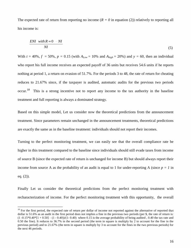
The expected rate of return from reporting no income (R = 0 in equation (2)) relatively to reporting all
his income is:
0ENI with R NI
NI (5)
With t = 40%, f = 50%, p = 0.15 (with ALow = 10% and Ahigh = 20%) and y = 60, then an individual
who report his full income receives an expected payoff of 36 units but receives 54.6 units if he reports
nothing at period 1, a return on evasion of 51.7%. For the periods 3 to 48, the rate of return for cheating
reduces to 21.67% since, if the taxpayer is audited, automatic audits for the previous two periods
occur.18
This is a strong incentive not to report any income to the tax authority in the baseline
treatment and full reporting is always a dominated strategy.
Based on this simple model, Let us consider now the theoretical predictions from the announcement
treatment. Since parameters remain unchanged in the announcement treatments, theoretical predictions
are exactly the same as in the baseline treatment: individuals should not report their incomes.
Turning to the perfect monitoring treatment, we can easily see that the overall compliance rate be
higher in this treatment compared to the baseline since individuals should still evade taxes from income
of source B (since the expected rate of return is unchanged for income B) but should always report their
income from source A as the probability of an audit is equal to 1 for under-reporting A (since p = 1 in
eq. (2)).
Finally Let us consider the theoretical predictions from the perfect monitoring treatment with
recharacterization of income. For the perfect monitoring treatment with this opportunity, the overall
18
For the first period, the expected rate of return per dollar of income not reported against the alternative of reported that
dollar is 51.6% as an audit in the first period does not implies a fine in the previous two periods (per $, the rate of return is:
(1 -0.15*0.40*[1 + 0.50] – (1 - 0.40))/(1- 0.40) where 0.15 is the average probability of being audited , 0.40 the tax rate and
0.50 the fine). It reduces to 36.7% in the second period (the term in square is multiply by 2 to account for the fine in the
previous period) and to 21.67% (the term in square is multiply by 3 to account for the fines in the two previous periods) for
the next 46 periods.

17
compliance rate should be close to the baseline treatment. The reason is that it is always optimal for a
participant to buy the maximum possible number of units of B with units of A. Indeed, purchasing
additional units of B costs 20% more than the units of B that the participants already own (buying
additional units of income B costs 1.20 units of income A). However, such recharacterization allows
the player to avoid the automatic auditing. The trade off between avoidance of automatic auditing and
paying an extra cost to buy additional units of B can be easily expressed in terms of expected rate of
return. Precisely, the expected rate of return of the purchased units of B is the same as the expected rate
of return for initial units of B minus the cost of purchasing extra units. The expected rate of return of
the purchased units of B is therefore 1.67% (i.e. 21.67% minus 20%). Thus it remains optimal to buy
extra units B and not reporting them. The expected rate of return for tax evasion for units of B that the
participants already own is unchanged at 21.67%.19
The predictions discussed above are from a very simple version of the Allingham- Sandmo – Yitzhaki
models. With the risk neutrality assumption, all the predictions lead to corner solutions of totally
avoiding tax by not reporting the non monitor incomes under all treatments.
A more realistic assumption is to assume that the taxpayer is risk averse. Here the first order condition
leads to interior solution in all treatments. If the expected penalty rate in less than the regular tax rate,
tax evasion remains an optimal strategy for the taxpayer. The monitoring treatments lower the gross
income space that should reduce tax evasion in the context of the A-S model. There is no argument,
however, to predict a change in the concavity of the utility function in those treatments.
Social and moral considerations will also bring people to refrain from tax evasions. This point is well
discussed in McCaffery and Slemrod (2004) in the context of behavioural public finance.
19
Note that because an individual cannot pay twice for non reporting her income if audited, therefore when one is hit by an
audit, the expected rate of return of cheating is the maximum of 51.6%, reaching 31.6% in the perfect monitoring treatment
with recharacterization of income for the purchased units of B.

18
Recently, authors have referred to non expected utility models to explain why people pay or decide not
to pay taxes (see for example, Dhami and al-Nowaihi, 2007, referring to prospect theory). The next
section will consider this approach in the context of behavioral predictions.20
4.2 Behavioral predictions
A possible objection to the expectation of a positive relationship between compliance and perfect
monitoring without recharacterization of income is that individuals may counteract the consequences of
a policy change to perfect monitoring, by taking on more risks by declaring less of their imperfectly
monitored income. Such an effect is akin to the idea of reference point in prospect theory.21
According
to loss aversion in prospect theory and the reference-dependent effect, individuals will try to recover
their losses following any policy changes, which may mean taking more risks. This is a familiar finding
among gamblers and traders who set specific financial targets.22
Our conjecture is stated more precisely
in H1.
H1: The increase in tax revenue due to the implementation of perfect monitoring on income of one
class (Source A) may be offset by reporting less income from another class (Source B).
Our second conjecture is that, for similar reasons as presented above, some participants may report less
income in the announcement treatment than in the baseline treatment in order to get a head start on
offsetting the future tax burden of the perfect monitoring policy. This is summarized in H2.
20
It is outside the scope of this paper to formalize those models. 21
The reference point consists of the individual's point of comparison against which each alternative is compared. In our
case, this can be the initial outcome obtained in the baseline treatment. According to the prospect theory, individuals will
'code' each alternative as a gain or a loss in utility relative to this reference point rather than using the absolute value of the
outcome. The resulting losses or gains are then weighed by their perceived probabilities of occurrence, forming a non-linear
value function. Because people typically approach gains and losses differently, generally acting risk-averse on gains and
risk-seeking on losses (Kahneman and Tversky, 1979), the result is a non-linear utility function. 22
A similar situation is with the concept of a target income and the behavioral model of labor supply developed by Altman
(2001). See also Camerer et al (1997) on income target related to the supply of taxis.

19
H2: Participants may be willing to counteract the future consequences of the perfect monitoring policy
by reporting less income in the current announcement treatment than in the baseline.
Audit experience may also influence perceptions of future audits, which is theoretically incorrect since
instructions of the experiment made it clear that audits were randomly assigned each period, not
conditionally on past behavior. A possible reason for this misperception is that a participant‟s attention
may be occupied with the bad outcome itself and neglect the fact that such event is very unlikely to
occur. This effect is generally termed the “probability neglect” effect. The idea is that, “when intense
emotions are engaged, people tend to focus on the adverse outcome, not on its likelihood, which may
lead to significant distortions in both private and public arenas” (Sunstein, 2002 p.61). Moreover
people may feel a disproportionate fear of risk when the associated risks are hard to control (Slovic,
2000; Sustein, 2002). Finally, the occurrence of an audit may also induce the opposite effect, by
provoking individuals to underestimate future audits. This effect, generally termed the “Gambler‟s
fallacy” or “Monte Carlo fallacy”, relies on the impression that a certain stochastic event is less likely
to happen following the occurrence of an event or a series of events. Again, this is obviously a fallacy
since the occurrence of past events do not impact the probability that similar random event will occur
in the future. According to Tversky and Kahneman, Gambler's fallacy may be induced by a
psychological heuristic.23 This is stated in H3.
H3: Audit experience may influence perceptions of risk and therefore influence current decisions.
In addition to risk perception, other behavioral factors may also influence tax compliance. For example,
some individuals may desire to conform to a norm of truth-telling. So called honest individuals would
23
The intuition behind Gambler fallacy is that people may expect that deviations from average should balance out. For
example, if a fair coin is tossed repeatedly and tails comes up a larger number of times than is expected, a gambler may
incorrectly believe that this means that heads is more likely in future tosses. Such an event is often referred to as being
"due".
20
avoid the emotional cost associated with deviation from this norm by reporting a non null part or all of
their income (Coricelli et al, 2008). This is summarized in assumption H4.
H4: Irrespective of pecuniary incentives, non-pecuniary factors such as norms of truth-telling may
motivate subject to report non null amounts of income in both the baseline and the announcement
treatments.
5. Experimental Results
5.1 Descriptive statistics
Figures 1a and 1b show the time path of the average reporting rates by period, in the different
treatments for sessions 1-8 (without recharacterization of income) and sessions 9-16 (with
recharacterization of income), respectively. The average reporting rate is shown on the vertical axis.
The period number is given on the horizontal axis. To facilitate comparisons across treatments, average
reporting rates are depicted graphically one the same time scale.
Average reporting rates are significantly different from zero in contradiction with the simple version of
the A-S-H models. Both figures indicate that in most treatments, reporting rates are rather stable over
time. Comparing treatments, both figures indicate important differences. Figure 1a shows that the
announcement phase induces a significant reduction of overall reporting rate. Introducing monitoring
policy without recharacterization of income does not lead to improve reporting rates. In contrast, Figure
1b shows that introducing perfect monitoring with recharacterization of income induces a negative
effect on the reporting rate level. Figure 1b indicates that the negative effect of announcement seems to
be lower in sessions 9-16 than in sessions 1-8. These results seem to confirm the idea that introducing a
perfect monitoring policy does not necessarily lead to an improvement of tax compliance because
21
agents may be willing to counteract the effects of such policy by reporting less income from other
sources, which translates into less overall reporting rate. In general, those results support our behavioral
predictions.
Table 1 presents descriptive statistics on the basic variables related to our experimental parameters and
behaviors exhibited by the participants (definition and construction of all the variables are presented in
appendix A). It shows that the reporting rate significantly decreases with perfect monitoring and
recharacterization of income. The reporting rate is 76.59% in the baseline treatment.24
This percentage
falls to 70.30% in the monitoring treatment with recharacteriezation of income and is significantly
lower than the baseline result (z = 4.452; p = 0.0001, Wilcoxon signed-rank tests). In contrast, we find
no significant difference between the baseline treatment and the monitoring treatment without
recharacterization of income (z = -0.490; p > 0.1). We also observe that the reporting rate is
significantly lower in the announcement stage preceding monitoring without recharacterization of
income (67.67%) compared to the baseline treatment (z = 3.456; p = 0.0005, Wilcoxon signed-rank).
We speculate that the difference in behavior between the two treatments is that the participants are
trying to counteract the expected consequences of the perfect monitoring policy by taking advantage of
their current situation. In contrast no significant difference is found between the baseline treatment and
the announcement treatment with opportunity of recharacterization of income (z = 0.941; p > 0.1). A
possible explanation is that participants anticipate that they can avoid future taxes under the
implementation of perfect monitoring when recharacterization is permitted. Consequently, they are not
motivated to “stock up” before the new policy is implemented. The non parametric tests confirm the
previous findings.
[Table 1, Figures 1a and 1b about here]
24
Note that a Mann-Whitney-Wilcoxon test indicates no significant difference between the two baseline treatments in
sessions with and without recharacterization of income (z = 1.131; p > 1).
22
In addition to the differences in the overall reporting rate across the treatments discussed above, we
also observe that the zero compliant participants, although small in number, are more numerous in the
monitoring treatment with recharacterization of income (1.55%), than the monitoring treatment without
recharacterization of income (0.05%). Figures 2a and 2b offer information about the effects of
announcement and monitoring with respect to level of income for sessions 1-8 (perfect monitoring
without the opportunity to recharacterize income) and sessions 9-16 (perfect monitoring with the
opportunity to recharacterize income), respectively.
[Figures 2a and 2b about here]
As illustrated in Figures 2a and 2b, reporting in the baseline is greater than 70% for every income
range. Given the substantial incentives to under-report, positive and relatively high reporting rates
indicate that the participants are either generally quite risk averse or that other suggested models of tax
compliance are at play here. As the stakes increase, we also observe that, in all treatments, reporting
rate decreases with the level of income.
Figure 2a shows that the announcement induces a significant reduction of overall reporting rate. In
contrast, perfect monitoring without opportunity to recharacterize income seems to have two opposing
effects depending on the level of income. An increase in monitoring seems to have a negative effect on
reporting rate for lower incomes whereas it has a positive effect on this ratio for higher incomes. With
Figure 2b, we observe that perfect monitoring with recharacterization of income induces a reduction in
the reporting rate level. Consistent with our previous results, the negative effect of announcement is
lower in this case compared to figure 2a, which indicates that subjects are aware that the introduction of
perfect monitoring is less dramatic when they have the opportunity to recharacterize income. Finally,
the negative effect of perfect monitoring (significant at 5%), compared to the baseline treatment,

23
indicates that increasing monitoring does not necessarily improve the reporting rates when individuals
have the opportunity to recharacterize income.
Table 2 provides, by participant‟s income type and policy treatment, descriptive statistics on income,
reported income, taxes paid, percentage of auditing, etc. Table 2 shows that the participants who had
80% of their income generated from Source A were obliged to report more income than they would
have if not monitored so closely.
[Table 2 and Figure 3 about here]
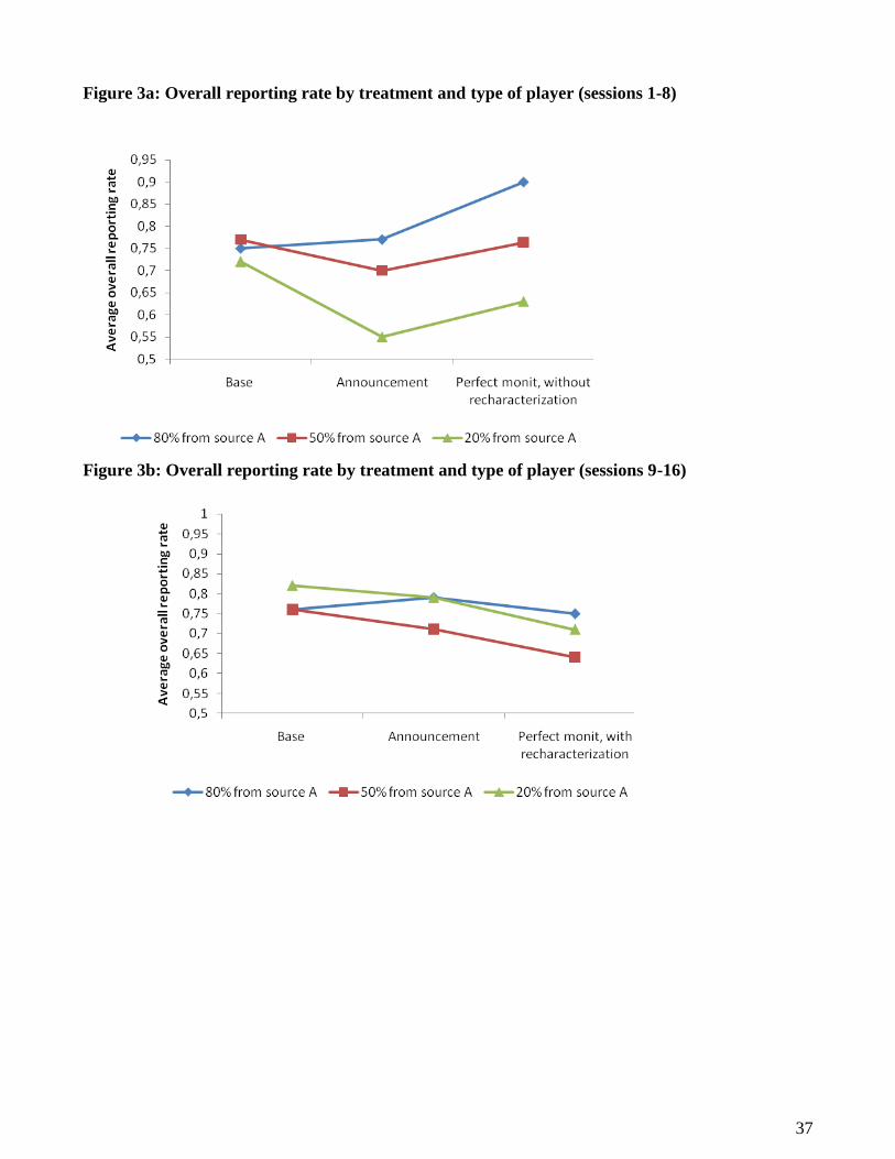
Figures 3a and 3b provide information concerning reporting rates for the three types of players across
all three experimental phases with and without recharacterization of income, respectively. Figure 3a
shows that without recharacterization of income, highly monitored participants who had 80% of their
income from Source A tend to increase their reporting rate on average in the monitoring treatment and
in the announcement treatment compared to the baseline treatment. In sharp contrast for the other two
types of participants (e.g. with 50% and 20% of income from source A), the reporting rates decline
through the announcement stage and move back upward throughout the perfect monitoring treatment.25
When future recharacterization is possible (Figure 3b), highly monitored participants tend to stabilize
their reporting rates while the other two types of participants significantly reduce them in the
announcement and the monitoring treatments.
Figures 4, 5 and 6 compare the two monitoring treatments with and without recharacterization of
income for each participant‟s income type. For those with 80% and 50% of income from Source A
(Figures 4 and 5), the declaration rates are generally lower for higher income levels and especially
when participants had the opportunity to transfer income from Source A to Source B. For the least
monitored participants, those with only 20% of total income derived from Source A, the difference

24
between the two treatments is insignificant. The participants‟ inclination to avoid being in the reported
income‟s lower bracket and by the same token to face a 20% auditing rate, explains this result.
Actually, since buying extra units of B is costly, it would be useless to do so if one had to report it. The
participant knows that, having 80% of his or her total income already not systematically audited, part of
this income will have to be reported to try to avoid the higher auditing rate.
[Figures 4, 5 and 6 about here]
5.2 Econometric results
The descriptive statistics imply that the perfect monitoring of matched income does not bring in greater
tax revenues for the government.26
In fact, tax revenues will decrease with perfect monitoring with
respect to the parameters of the experiment. Two primary factors can explain this result.
First, as the descriptive statistics for the monitoring treatment without recharacterization of income
show, participants tend to cheat more on unmonitored income when they cannot under-report
monitored income. The only exception in this study is the subgroup of participants whose income from
Source A represents 80% of their total income. Second, there is a shift towards unmonitored income
(Source B) when this option is available for the highly monitored participants (80% and 50% from
Source A). A reasonable explanation for these observations is that participants are willing to assume
more risks when they are closely monitored in order to maintain a net expected income comparable to
what they had before the introduction of monitored income.
In this section, the data are analysed with parametric regressions. Table 3 consists of two panels. The
left panel displays the result of five regressions in which the dependent variable is the percentage of
total income reported to the tax authority by individual i at period t. It shows the estimates of the
25
Alm and McKee (2006) found that announcement increases compliance of those told they will be audited, but reduces
compliance of those knowing they will not be audited; the net effect is that overall compliance falls.

25
determinants of reporting rates by treatment with random effects Tobits.27
The use of Tobit models is
justified by the number of left and right censored observations in the sample. The right panel (column
6) presents the results of the determinants of tax revenue from a random effects Feasible-Generalized-
Least-Squares regression.28
We control for demographics (not reported in the estimates but available
upon request).29
The estimates support earlier observations that tax reporting declines with total income level. We also
observe that the participants reduce their reported income in the period following an audited period.
This reaction to previous audit is in accordance with our discussion on optimal strategy. This result is
also consistent with the reference-dependence effect in prospect theory. Participants may be willing to
compensate for the losses suffered in the audit, even at the expense of taking more risks (Tversky and
Kahneman 1991). This occurrence could also be explained by the “Gambler’s fallacy” concept, which
states that the participants believe that after being audited once, the probability to be audited again soon
after is smaller than the described probability. This is of course incorrect, the auditing probabilities
being independent from a period to the next.30
Columns (1) and (2) indicate that there is no significant
26
Tax revenues are the tax paid on the reported income. They do not include penalties. 27
In a panel Tobit, the error component splits into a time invariant individual random effect, i and a time-varying
idiosyncratic random error it .
28 Given itRF measuring the taxes paid (tax revenues) by participant i at period t. Tax revenues are described by a vector
of exogenous variables zit and the corresponding vector with parameters , and a random variable that can be divided into a
random individual effect i , and a pure random variable it : , 1, , , 1, ,it it i itRF z i n t T ,
Assuming uncorrelated errors terms and that the zit are also uncorrelated with the errors terms, an appropriate estimation
technique is the Feasible-Generalized Least-Squares discussed in Greene (2008, chapter 9). 29
Demographics include various participant characteristics: age (mean: 25.4; sd: 5.95); male (53.1%) previous participation
is a binary variable for whether the participant has already taken part in an experiment other than the current one (1=
participated in a previous experiment (38.5%), 0 otherwise,); gamble indicates whether the participant chose to earn a
guaranteed $5 show-up fee or a gamble with a 50% probability of earning $11 and a 50% probability of earning $0.
Participants who choose the gamble are considered relatively less risk averse than those who chose the $5 show-up fee
(73.4%); instruction feedback describes the participant‟s assessment of the clarity of the instructions on a scale of 0 to 10,
10 being “very clear” (mean: 8.29; sd:1.46); and a list of binary variables indicating whether the participant is a worker
(8.85%), unemployed (6.25%), a student (80.2%), a graduate student (22.4%) or a student with prior mathematical training
(66.1%)). The introduction of demographic variables does not affect the estimated coefficients of the experimental
variables. Most of these variables are not statistically significant. 30
Here behavioral economics is an explanation of the results and not the basis for a policy recommendation. McCaffery
(2006) has discussed in the context of policies aimed at increasing the saving rate in the US, the marriage of behavioral
economics and fundamental tax reform.
26
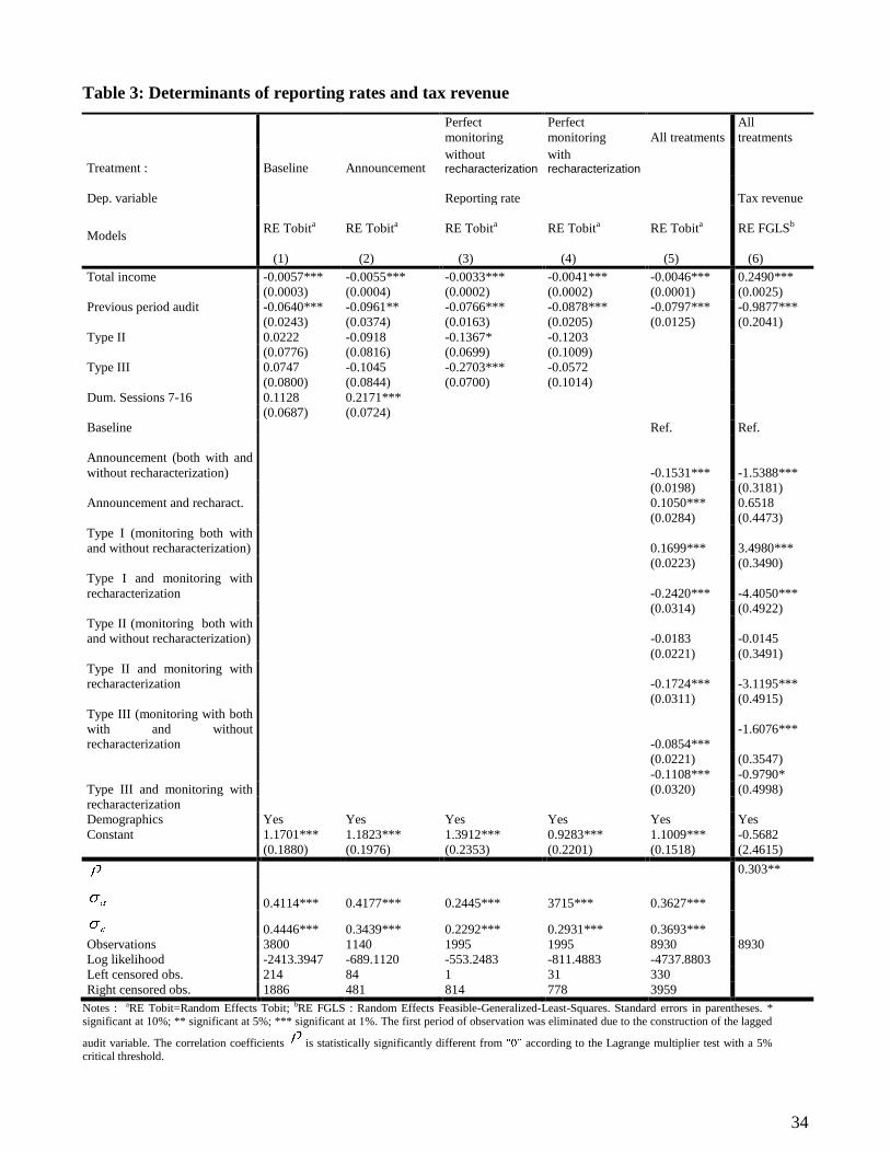
difference among player types in the baseline and announcement treatments. In contrast, as shown by
column (3), the perfect monitoring treatment without recharacterization of income reveals that players
of types II and III report significantly less than players of type I, which is consistent with our previous
findings. The lower constant term suggests that on average, people report less income in the perfect
monitoring treatment with opportunity to recharacterize income.
With respect to the reference variable that is the baseline treatment preceding the announcement and
policy implementation treatments, column (5) reveals that the tax rate reporting decreases for all types
of players under perfect monitoring when transfers from Source A to Source B income are permitted. If
the participants are not able to shift income from Source A to Source B, the tax reporting increases for
those participants with 80% of their initial income coming from Source A under perfect monitoring
when compared to the baseline treatment. The tax rate reporting is stable for participants with 50% of
their income coming from Source A and decreases for those with 20% of their income coming from
Source A.
In the announcement treatment preceding the perfect monitoring without recharacterization of income,
the tax rate reporting decreases with respect to the baseline treatment. In the announcement treatment
preceding the introduction of the perfect monitoring with the opportunity to recharacterize income,
there is no diminution in tax reporting as already noted earlier.
[Table 3 about here]
Turning to the determinants of tax revenues, column (6) reports a positive and significant coefficient
associated to the “total income” variable. We have seen earlier that the reporting rates decrease with the
income level. Nonetheless, column (6) shows that tax revenues increase with the income since the
income raise compensates for the diminution of the reported income. Consistent with our previous

27
results, column (6) shows that the tax revenues decrease under perfect monitoring with characterization
compared to the baseline. The tax revenues decrease by 0.907 eu, 3.134 eu and 2.5866 eu with respect
to the baseline treatment for participants with respectively 80%, 50% and 20% of their initial income
coming from Source A.31
If the participants are not allowed to shift income from Source A to Source B,
the tax revenues increase by 3.498 eu for those participants with 80% of their initial income coming
from Source A under perfect monitoring when compared to the baseline treatment. Tax revenues are
stable for participants with 50% of their income coming from Source A and they decrease by 1.607 eu
for those with 20% of their income coming from Source A.
6. Conclusion
This study examines the impact on tax compliance of perfect monitoring of a single source of income,.
using a laboratory experiment to observe actual and reported incomes in a repeated-decision
framework. The background application is the sales taxes. Two treatments were used to observe the
differences in responses to monitoring, with and without the opportunity to recharacterize income from
the perfectly monitored source to an alternative unmonitored source.
Our experiment contributes to the previous existing literature on tax compliance by showing that
increasing the probability of audit does not necessarily lead to a reduction of tax evasion, because
taxpayers may offset the revenue gain of an increased probability of audit of one source of income by
reporting less income from other sources that are less monitored (a reference-dependent effect), and by
recharacterizing closely monitored income as an alternative less-monitored source of income when
such recharacterizing is possible. This result is consistent with Gerxhani and Schram (2006) who found
a significant shift from perfectly monitored income towards less-monitored income when tax evasion is
31
To illustrate for the type II participant: with respect to the reference state, we add the coefficient -0.0145 of type II (both
treatments)” to the coefficient – 3.1195 of “Type II and recharacterization”.

28
made possible. It is also in line with Alm et al. (2009), who suggest that the amount of tax evasion is
greater for individuals with non-matched income.
We have three key findings.
First, on average, the less monitored income types (50% and 20% of income comes from the perfectly
monitored Source A) and all income types when the option to alter the sources of income was allowed
had higher rates of noncompliance. The only group that had the same rate of compliance was the group
of participants who derived 80% of their income from Source A and had no opportunity to
recharacterize incomes.
Second, when participants had the opportunity to recharacterize perfectly monitored income, they more
than compensated for the unavoidable taxes on Source A income by reporting less unmonitored income
(from Source B).
Third, we find a significant decrease in tax revenues if income can be recharacterized (at a cost). In this
case, we observe approximately a 15 percent decline in tax revenues. We are not claiming that a 15%
tax reduction in tax revenues would be observed with such a reform, but our experiment suggests that,
if perfect monitoring is instituted without some other complementary policies, an increase in tax
revenues is not the likely outcome.
Our study stresses that a successful policy aimed at reducing fiscal fraud might be difficult to design if
taxpayers have determined an equilibrium level of tax compliance. One potential explanation, which
draws on the reference-dependent effect and loss aversion in prospect theory, suggests that individuals
will try to recover their losses following any policy changes even if it means taking more risks.

29
This seems far too strong for what you have shown: Maybe the only solution is to assess what
taxpayers consider a “fair” level of taxation, which balances their relative level of tax contributions
with what they expect to gain from them.

30
References
Allingham, M.G., and A. Sandmo, “Income Tax Evasion: A Theoretical Analysis.” Journal of
Public Economics 1. (November) 1972: 323-338.
Alm. J., B.R. Jackson, and M. McKee “Estimating the Determinants of Taxpayer Compliance with
Experimental Data.” National Tax Journal 45. (March) 1992: 107-114.
Alm, J., C. Blackwell, and M. McKee, ¨Audit Selection and Firm Compliance with a Broad-based
Sales Tax.¨ National Tax Journal 57. (June) 2004: 209-227.
Alm J., J. Deskins, and M. McKee, ¨Do Individual Comply on Income Not Reported by Their
Employer?¨ Public Finance Review 37. (March) 2006: 120-141.
Alm J., and M. McKee, ¨Audit Certainty, Audit Productivity and Taxpayer Compliance.¨ National
Tax Journal 59. (December) 2006: 801-816.
Alman M. ¨A Behavioral Model of Labor Supply: Casting some Light into the Black Box of
Income-leisure Choice¨. The Journal of Socio-Economics. 2001: 199-219.
Andreoni. J., B. Erard, and J. Feinstein, “Tax Compliance.” Journal of Economic Literature 36.
(June) 1998: 818-860.
Boylan, S., and G. Sprinkle. ¨Experimental Evidence on the Relation between Tax Rates and
Compliance: The Effect of Earned vs. Endowed Income. Journal of the American Taxation Association
23 (1). 2001: 75-90.
Bruce, Donald. Effects of the United States Tax System on Transitions Into Self-employment. Labour
Economics 7. 2000: 545-574.
Cadsby C.B., E. Maynes, and V.U. Trivedi, „Tax compliance and obedience to authority at home
and in the lab: A new experimental approach‟ Experimental Economics 9. 2006:343-359.
Camerer C., F., L. Babcock, G. Loewenstein, and R. Thaler. "Labor Supply of New York City Cab
Drivers: One Day at a Time." Quarterly Journal of Economics 111. 1997: 408-41.
Clotfelter, C. ¨Tax Evasion and Tax Rates: An Analysis of Individual Returns.¨ Review of Economics
and Statistics 65 (3). 1983: 363-373.
Coricelli, G., M. Joffily, C. Montmarquette, and M.C. Villeval “Cheating and Emotional Rationality:
An Experiment on Tax Evasion”, Cirano Working paper, 2008.
Dubin. J. A., M.J. Graetz, and L.L. Wilde. “The Effect of Audit Rates on the Federal Individual
Income Tax. 1977-1986.” National Tax Journal 43(4). 1990: 395-409.
Dhami S., and A. Al-Nowaihi ¨Why do people pay taxes? Prospect theory versus expected utilily
theory¨, Journal of Economic Behavior & Organization 64 (1). (September) 2007: 171-192.

31
Erard, B., and C. Ho (2001). ¨Searching for Ghosts: Who Are the Nonfilers and How Much Tax Do
They Owe?¨ Journal of Public Economics 81. 2001: 25-50.
Feinstein, J. S. ¨An Econometric Analysis of Income Tax Evasion and its Detection¨. RAND Journal of
Economics 22 (1). 1991: 14-35.
Fortin B., G. Garneau, G. Lacroix, T. Lemieux, and C. Montmarquette. “L'économie souterraine au
Québec” Mythes et réalités, Sainte-Foy: Presses de l‟Université Laval. 1996.
Friedland, N., S. Maital, and A. Rutenberg. “A Simulation Study of Income Tax Evasion”.Journal
of Public Economics, 10. 1978: 107-116.
Gërxhani K., and A. Schram. ¨Tax evasion and income source: A comparative experimental study¨.
Journal of Economic Psychology 27( 3). 2006: 402-422.
Greene W. Econometric Analysis. Prentice Hall, 6th
edition. 2008.
Internal Revenue Service. Federal Tax Compliance Research: Individual Income Tax Gap
Estimates for 1985. 1988. and 1992. IRS Publication 1415 (Rev. 4-96). Washington. D.C. 1996.
Jackson B.R., and V.C. Milliron. ¨Tax compliance research: Findings, problems and prospects¨.
Journal of Accounting Literature 5. 1986: 125–165.
Joulfaian, D., and M. Rider. Differential Taxation and Tax Evasion by Small Business. National Tax
Journal 51 (4). 1998: 676-687.
Kahneman D., and A. Tversky. ¨Judgment under uncertainty : Heuristics and Biases¨. Science. 185.
1974 1124-1130.
Kahneman D., and A. Tversky."Prospect Theory: An Analysis of Decision under Risk". Econometrica
47. 1979: 263-91.
McCaffery E.J. ¨Behavioral Economics and Fundamental Tax Reform¨, USC Center in Law,
Economics and Organization Research Center. 2006: C06-4.
McCaffey E.J., and J. Slemrod ¨Toward an agenda for behavioural public finance¨, in E.J. McCaffey,
and J. Slemrod (eds), Behavorial Public Finance, Russell Sage Foundation: New York. 2006, 3-32.
Mikesell J.L. ¨Audits and the tax base: Evidence on Induced sales tax noncompliance¨. Western Tax
Review 6. 1985: 86-114.
Murray M.N. "Sales Tax Auditing and Compliance". National Tax Journal 48. 1995: 515-530.
Lippert O., and M. Walker. Editors. The Underground Economy : Global Evidence of Its Size and
Impact. Fraser Institute. 1997.
Roth J.A., and J.T Scholz, Editors, Taxpayer Compliance, Volume 2, Social Science Perspectives.
University of Pennsylvania Press: Philadelphia. 1989.
32
Slemrod J., M. Blumental, and C. Christian “The Determinants of Income Tax Compliance:
Evidence From a Controlled Experiment in Minnesota.” Journal of Publics Economics 79(3). 2001:
455-483.
Slemrod, J. Why People Pay Taxes: Tax Compliance and Enforcement. University of Michigan Press:
Ann Arbor MI. 1992.
Slovic, P. The Perception of Risk. London: Earthscan Publications. 2000.
Sunstein, C. “Probability Neglect: Emotions, Worst Cases, and Law,” Yale Law Journal 112. 2002:
61–107.
Webley P., H. Robben and H. Effers and D. Hessing. Tax Evasion: An Experimental Approach.
CambridgeUniversity Press: Cambridge. 1991.
Yitzhaki, S. A note on 'Income Tax Evasion: A Theoretical Analysis'. Journal of Public Economics
3(2). 1974: 201-202.

33
Table 1: Descriptive statistics by treatment*
VARIABLES
Monitoring treatment without recharacterization of income:
Sessions (1-8)
Monitoring treatment with recharacterization of
income: Sessions (9-16)
Type I
80% Source A
Type II
50% Source A
Type III
20% Source A
Type I
80% Source A
Type II
50% Source A
Type III
20% Source A
Average Std Dev. Average Std Dev. Average Std Dev. Average Std Dev. Average Std Dev. Average
Std
Dev.
Total income 58.02 27.18 58.02 27.18 57.75 27.15 59.33 28.53 59.33 28.53 59.49 28.43
Reported income 52.11 24.51 43.70 24.00 34.47 23.84 43.53 26.17 35.63 26.27 41.32 28.86
Overall reporting rate (%) 90.38% 9.72% 76.44% 22.48% 63.57% 33.90% 75.52% 28.16% 64.01% 35.80% 71.41% 35.20%
Reporting rate on B * (%) 54.23% 44.76% 53.49% 44.22% 54.97% 41.83% 44.97% 45.28% 52.19% 42.65% 67.98% 38.70%
Taxes paid on the reported income 20.63 9.81 17.21 9.37 13.60 9.65 17.23 10.51 14.04 10.59 16.40 11.63
Amount of B purchased 7.74 14.32 7.93 11.25 2.89 4.58
Amount B purchased / Amount B
available 17.99% 30.11% 30.00% 38.21% 26.83% 38.26%
% reporting no income 0.15% 0.89% 1.93% 1.84%
% reporting their total income 42.41% 41.82% 35.33% 37.50% 34.08% 43.93%
% reporting no income on B 29.76% 27.53% 17.67% 36.01% 17.86% 15.51%
% Auditing 14.29% 12.80% 15.05% 14.88% 18.60% 14.90%
* (reported income – income from Source A) (income from Source B)
Table 2: Descriptive statistics by income type and monitoring treatment
* (reported income – income from Source A) (income from Source B)
VARIABLES
All income reported in eu
Baseline treatment (both sessions 1-8 and
9-16)
Announcement preceding
monitoring without recharacterization
of income: (sessions 1-8)
Announcement preceding monitoring
with recharacterization
of income: (sessions 9-16)
Perfect Monitoring
treatment without recharacterization
of income: (sessions 1-8)
Perfect Monitoring treatment with
recharacterization of income
(sessions 9-16)
Average Std Dev. Average Std Dev. Average Std Dev. Average Std Dev. Average Std Dev.
Total income 60.96 28.74 52.62 27.99 62.45 30.40 57.93 27.16 59.38 28.48
Reported income 45.54 29.89 34.64 26.80 45.63 29.33 43.52 25.16 40.15 27.30
Overall reporting rate (%) 76.59% 32.64% 67.67% 36.58% 76.56% 30.72% 76.94% 26.38% 70.30% 33.54%
Reporting rate on B * (%) 63.66% 43.58% 52.05% 44.97% 59.30% 43.68% 54.22% 43.62% 54.91% 43.38%
Taxes paid on the reported income 17.95 11.84 13.69 10.75 17.99 11.76 17.18 10.02 15.88 10.99
Amount B purchased 6.22 11.13
Amount B purchased / Amount B available 24.92% 36.05%
% reporting no income 5.51% 9.82% 4.91% 0.05% 1.55%
% reporting total income 47.54% 39.12% 42.81% 39.90% 38.45%
% reporting no source B income 26.44% 31.75% 25.44% 25.06% 23.21%
% Auditing 14.31% 13.51% 13.51% 14.04% 16.14%
34
Table 3: Determinants of reporting rates and tax revenue
Treatment : Baseline Announcement
Perfect
monitoring
Perfect
monitoring All treatments
All
treatments
without recharacterization
with recharacterization
Dep. variable
Reporting rate
Tax revenue
Models RE Tobita RE Tobita
RE Tobita
RE Tobita
RE Tobita
RE FGLSb
(1) (2) (3) (4) (5) (6)
Total income -0.0057*** -0.0055*** -0.0033*** -0.0041*** -0.0046*** 0.2490***
(0.0003) (0.0004) (0.0002) (0.0002) (0.0001) (0.0025)
Previous period audit -0.0640*** -0.0961** -0.0766*** -0.0878*** -0.0797*** -0.9877***
(0.0243) (0.0374) (0.0163) (0.0205) (0.0125) (0.2041)
Type II 0.0222 -0.0918 -0.1367* -0.1203
(0.0776) (0.0816) (0.0699) (0.1009)
Type III 0.0747 -0.1045 -0.2703*** -0.0572
(0.0800) (0.0844) (0.0700) (0.1014)
Dum. Sessions 7-16 0.1128 0.2171***
(0.0687) (0.0724)
Baseline Ref. Ref.
Announcement (both with and
without recharacterization) -0.1531***
-1.5388***
(0.0198) (0.3181)
Announcement and recharact. 0.1050*** 0.6518
(0.0284) (0.4473)
Type I (monitoring both with
and without recharacterization) 0.1699***
3.4980***
(0.0223) (0.3490)
Type I and monitoring with
recharacterization -0.2420***
-4.4050***
(0.0314) (0.4922)
Type II (monitoring both with
and without recharacterization) -0.0183
-0.0145
(0.0221) (0.3491)
Type II and monitoring with
recharacterization -0.1724***
-3.1195***
(0.0311) (0.4915)
Type III (monitoring with both
with and without
recharacterization -0.0854***
-1.6076***
(0.0221) (0.3547)
Type III and monitoring with
recharacterization
-0.1108*** -0.9790*
(0.0320) (0.4998)
Demographics Yes Yes Yes Yes Yes Yes
Constant 1.1701*** 1.1823*** 1.3912*** 0.9283*** 1.1009*** -0.5682
(0.1880) (0.1976) (0.2353) (0.2201) (0.1518) (2.4615)
0.303**
0.4114*** 0.4177*** 0.2445***
3715*** 0.3627***
0.4446*** 0.3439*** 0.2292*** 0.2931*** 0.3693***
Observations 3800 1140 1995 1995 8930 8930
Log likelihood -2413.3947 -689.1120 -553.2483 -811.4883 -4737.8803
Left censored obs. 214 84 1 31 330
Right censored obs. 1886 481 814 778 3959
Notes : aRE Tobit=Random Effects Tobit; bRE FGLS : Random Effects Feasible-Generalized-Least-Squares. Standard errors in parentheses. * significant at 10%; ** significant at 5%; *** significant at 1%. The first period of observation was eliminated due to the construction of the lagged
audit variable. The correlation coefficients is statistically significantly different from according to the Lagrange multiplier test with a 5% critical threshold.

35
Figure 1a: Overall reporting rate by treatment over time (sessions 1-8)
Figure 1b: Overall reporting rate by treatment over time (sessions 9-16)

36
Figure 2a: Ratio of reported income per level of income (session 1-8)
Figure 2b: Ratio of reported income per level of income (session 9-16)
37
Figure 3a: Overall reporting rate by treatment and type of player (sessions 1-8)
Figure 3b: Overall reporting rate by treatment and type of player (sessions 9-16)

38
Figure 4: Ratio of the reported income for those having 80% of their income automatically audited (Source A)
Figure 5: Ratio of the reported income for those having 50% of their income automatically audited (Source A)
Figure 6: Ratio of the reported income for those having 20% of their income automatically audited (Source A)

39
Appendix A: Definitions of Variables
Name Definition
Basic (Baseline)
Announcement
Announcement with recharacterization
Announcementwithout recharacterization
Monitoring with recharacterization
Monitoring without recharacterization
Perfect monitoring
Type I
Type II
Type III
Type i and Monitoring
Total income
Reported Income
Overall reporting rate
Audit
Age
Men
Previous participation
Gamble
Instruction Feedback
Worker
Unemployed
Student
Graduate student
Mathematical training
1 if Baseline treatment is played and 0 otherwise
1 if Announcement treatment is played and 0 otherwise
1 if Announcement treatment preceding monitoring with the option to alter is played and
0 otherwise.
1 if Announcement treatment preceding monitoring without the option to alter is played
and 0 otherwise.
1 if Monitoring with the option to alter treatment is played and 0 otherwise
1 if Monitoring without the option to alter treatment is played and 0 otherwise
1 if Monitoring is possible (i.e in monitoring treatments with and without option to alter)
and 0 otherwise
Player‟s source A income is 80% of her total income
Player‟s source A income is 50% of her total income
Player‟s source A income is 20% of her total income
Interaction variables
Player‟s income randomly drawn between 10 and 110 experimental units.
Reported income by each player
Reported income/total income
1 if the participant is audited and 0 otherwise
Player‟s age
1 if participant is a male and 0 otherwise.
1 if the player has already taken part in an experiment other than the current one and 0
otherwise
1 if the participant chose a gamble (50% probability of earning $11 and a 50% probability
of earning $0) and 0 if she chose to earn a guaranteed $5 show up fee.
Describes the participant‟s assessment of the clarity of the instructions (from 0 to 10)
1 if the participant is a worker and 0 otherwise
1 if the participant is unemployed and 0 otherwise
1 if the participant is a student and 0 otherwise
1 if the participant is a graduate student and 0 otherwise
1 if the student with prior mathematical training and 0 otherwise

40
Appendix B: Participant instructions (translated from French)
General Instructions
You are asked to participate in a series of decisions. This experiment is made of several periods. You will be
asked to make a decision in each period. You must complete one period before moving on to the next period.
Your earnings depend on what you decide. Therefore, it is important to read these instructions carefully.
At the end of the experimental session, you will make a random draw from all the played periods. Your earnings
for the session will be a function of your “net final income” from that period.
What you earn is completely private. You will be paid for one randomly selected decision (period) in private at
the end of the experiment.
Period Breakdown.
Every period, you will receive your income. This income is randomly drawn by the computer and is between 10
eu (experimental units) and 110 eu.
Two sources of income
Your income comes from two different sources: A and B.
There are three participant types randomly determined by the computer. They are characterized by whether most
of their income comes from source A, source B, or equally from both sources. That is
Type 1: 80 % of your total income comes from source A and 20 %, from source B.
Type 2: your total income comes equally from sources A and B.
Type 3: 20 % of your total income comes from source A and 80 %, from source B.
For example, suppose that you are a type 3 player. If your total income is 50 eu, 10 eu would come from source
A and 40 eu would come from source B. This information is confidential. You remain of the same type for the
entire experiment.
Paying taxes
Only you know your true income. Once you know your true income, you will be asked to report your income to
the government and pay taxes on the reported income. There is no restriction on how much you can report (apart
from it being a non-negative whole number – no decimals). You can report more, the same or less than your true
income.
Your earnings at the end of the experiment depend on your true income less taxes paid and possible fines. Once
you have reported your income, a 40% tax is levied on this reported income.
Auditing
The government does not know your true earned income nor whether your income from source A is 80%, 50%
or 20% of total income. Only you know this. The government could audit you and everyone else in the room and
discover your income, but this is very expensive and useless if you already reported your true income.
Therefore, the government randomly audits people and the probability to be audited is a function of the
following rule:
If your reported income is in the bottom 50% of the reported incomes, the probability to be audited is 20%.
If your reported income is in the top 50% of the reported incomes, the probability to be audited is 10%.
If you are audited and it reveals that you have under-reported your total income, you will have to pay:
1) the taxes on the non-reported income, and
2) a fine corresponding to 50% of the overdue taxes that you had not reported.
In other words, you would be paying one and half times the unpaid taxes.
Additionally, if audited, you will automatically be audited for the previous 2 periods. If you had under-reported
your income in these periods, you will have to pay 1.5 times the unpaid taxes for each one of these periods as
well. Hence, your “net final income” for the audited period is equal to your reported income less the taxes paid

41
on your reported income less the sum of the overdue taxes and fines for the current period (t) and the previous 2
(t-1 and t-2), if applicable.
Note that you can not be audited (and fined) twice for the same period.
How your earnings from the experiment are determined
Every period, your “net final income” is determined by the computer the following way:
If you are not audited: ”Final net income” = Total income – Taxes on the reported income
If you are audited and have reported your total income:
”Final net income” = Total income – Taxes on the reported income
If you are audited and have not reported your final income:
”Final net income” = Total income – Taxes on the reported income
– Taxes on the non-reported income (in t. t-1 and t-2) – Fines (in t. t-1 and t-2)
As a reminder, taxes on the reported income are 40% of the reported income, the taxes on the non-reported
income (payable if audited) correspond to: 40% X (total income – reported income). Finally, the fine
corresponds to 50% of the taxes on the non-reported income. (note that our program rounds up the decimals).
At the end of the experimental session, you will randomly draw a number corresponding to one of the played
periods. Each number has an equal probability to be drawn. Your earnings in eu for the drawn period will be
converted with a $1 eu = 0.50 $CAN rate.
Additional information
We recommend you to re-read these instructions. After taking place in front of your computer, please raise your
hand if you have questions regarding the instructions. We will come and answer them privately, and will then
inform everybody in the room of both the question and the answer. The questions should not try to validate a
decision strategy, but only attempt to understand the instructions better.
Before we start the experimental session, we will ask you some questions regarding your age, gender, level of
education and field of study, universities or schools currently attended, or your situation on the work market, and
whether you have already participated in such an experiment. This information will remain anonymous. We will
then begin the experiment.
We will also so ask you some comprehension questions on these instructions.
1st Announcement treatment. (sessions 1-8 ; given prior to period 22)
We are only advising you that starting 6 periods from now, a new technology will allow the government to
automatically know all the income you will earn from source A. However, as a reminder, the government
will not know your total income nor which type of player you are (i.e. whether your income from source A is
80%. 50% or 20% of your income).
Following the introduction of this technology, since the government will know all the income coming from
source A, you will be audited automatically if you report income less than what you receive from source A.
We remind you that, as in the previous periods, when you are audited for a given period, you will be
retroactively audited for the two previous periods as well. In other words, if you are audited in this upcoming
period, you will automatically be audited for the last two periods before this new technology was announced.
2nd
Perfect Monitoring (sessions 1-8 ; given prior to period 28)

42
As promised, the new technology that allows the government to automatically know all the income you will earn
from source A is in service.
From now on, if you report income lower than received from source A, you will be automatically audited.
The other conditions regarding the taxes, fines and audit are still in effect.
1st Announcement. (sessions 9-16 ; given prior to period 22
We are only advising you that starting 6 periods from now. a new technology will allow the government to
automatically know all the income you will earn from source A. However, as a reminder, the government
will not know your total income nor which type of player you are (i.e. whether your income from source A is
80%. 50% or 20% of your income). Furthermore, you will be able to purchase experimental units of source B
with units of source A, at the specified rate.
Following the introduction of this technology, since the government will know all the income coming from
source A, you will be audited automatically if you report income less than what you receive from source A.
We remind you that, as in the previous periods, when you are audited for a given period, you will be
retroactively audited for the two previous periods as well. In other words, if you are audited in this upcoming
period, you will automatically be audited for the last two periods before this new technology was announced.
2nd
Perfect Monitoring treatment with recharacterization. (sessions 9-16;given prior to period 28)
As promised, the new technology that allows the government to automatically know all the income you will earn
from source A is in service, you are able to purchase units of source B with units of source A. You must expend
1.20 units of A to obtain 1 unit of B. We specify that this technology allows the government to know your final
number of units from A, but it does not know how much you initially had. Without auditing you, the government
does not know your income from source B. If you decide to do such transactions, your gross income will be
modified, but your taxable income will remain your initial given income.
From now on, if you report income lower than received from source A, you will be automatically audited.
The other conditions regarding the taxes, fines and audit are still in effect.
If you have not purchased units of B with units of A, your “final net income” is calculated by the computer the
same way as before.
If you have purchased units of B with units of A. your “final net income” is calculated by the computer the
following way:
If you are not audited : “Final net income” = Total income – Cost to purchase units of B– Taxes on the reported income
If you are audited and have reported your total income:
“Final net income” = Total income – Cost to purchase units of B – Taxes on the reported income
If you are audited and have not reported your total income:
“Final net income” = Total income – Cost to purchase units of B – Taxes on the reported income – Taxes on the
non-reported (initial) total income (in t. t-1 and t-2) – Fines
(in t. t-1 and t-2)