The Effect of Off-farm Work on Production Intensity and Output Structure

Euan Phimister12 and Deborah Roberts1

1Arkleton Centre for Rural Development Research, University of Aberdeen. 2Department of Economics, University of Aberdeen. Postal Address: Department of Economics, University of Aberdeen, Aberdeen AB24 3QY. Email:e.phimister@abdn.ac.uk; deb.roberts@abdn.ac.uk. The permission of the Scottish Executive Environmental and Rural Affairs Department to access the data used in this paper is gratefully acknowledged. This is a revised version of a paper presented at Workshop on the Importance of the Household-firm Unit in Agriculture and Its implications for Statistics Wye College Imperial College, University of London April 2002. We would like to thank the participants for their useful comments. All usual caveats apply.

2

Introduction

The importance of off-farm earnings in helping maintain farm households is well recognized. As a result, research on the determinants and structure of off-farm labour supply has been extensive (for a review see Lass, Findeis and Hallberg). In comparison, with a few exceptions, the effect of off-farm labour on farm production decisions has received little attention from social scientists (Olfert; Olfert, 1993; Bokemeier and Garkovitch; Coughenour and Swanson; Gasson). However, such effects may be important as the justification for support increasingly emphasizes agriculture’s multifunctional role (Blandford and Boisvert; EU Commission 1999; 2000; Lindland, 1998). For example, if off-farm work does affect farm production decisions, policies that encourage the provision of off-farm employment opportunities may also impact upon the environmental services provided by farm households and vice-versa.

Two separate perspectives on the potential on-farm effects of off-farm employment are apparent from previous research. First, that off-farm labour supply is likely to have negligible effects on farm production decisions, because it is seen as a response to underemployment of farm labour (Olfert). That is, off-farm work is seen as ‘supplementary’ or residual activity undertaken after farm production decisions have been made (Carlin and Bentley). This view is also consistent with the qualitative evidence on the reluctance of farmers to take off-farm jobs (Shucksmith and Smith). In contrast, other evidence suggests that off-farm work is associated with higher levels of biodiversity, farm size and performance (Ellis et al; Coughenour and Swanson; Weiss). However, this research has not explicitly considered the simultaneous nature of off-farm work and production decisions. Rather, attention has tended to concentrate on the effect of individual preferences, e.g. attitudes to the environment and self-identity which are known to be important in farm production choices (Bokemeier and Garkovitch; Gasson; Willock et al).

The aim of this paper is to consider the effect of off-farm work on input and

output intensities and on the structure of farm output. Specifically, we econometrically estimate the impact of off-farm work on a number of output and input ratios using individual farm level panel data. The availability of panel data allows us to estimate a sample selection model that accounts for both unobserved heterogeneity and the potential simultaneity between farm production and off-farm work decisions (Vella and Verbeek; Nijman and Verbeek).

The paper adds to the literature in a number of ways. As discussed above

previous studies have typically not taken the potential simultaneous nature of the two decisions into account. Further, as our model allows for unobserved heterogeneity, we control for differences in productivities and household preferences across farms, so that estimated effects are not due simply to differences in these factors. Previous research on off-farm work decisions has used the implications of farm household models to guide their empirical work (Huffman). Clearly, the estimation of production effects of off-farm work should also derive from this type of economic framework. However, in developed countries the available farm level data is focused primarily on production and provides little information on other household characteristics (Hill). Hence, the extensive data requirements to estimate structural household models allowing for both production and off-farm work are often difficult to satisfy (Lopez). The panel data selection model used in this paper provides a method that controls for farm household characteristics and preferences in circumstances where such information is extremely limited.

3

The plan of the paper is as follows. In the next section we briefly consider the implications of the time allocation farm allocation model for output intensity. Section 3 describes the structure of the econometric models estimated and the approach taken to testing. In Section 4, the dataset is described. Section 5 reports estimation results. Section 6 concludes. Off-farm Work and Production Intensity To illustrate the implications of standard farm household models for production intensity, we consider a simple Nakajima time allocation model of a single person household with fixed capital, land and available time, T. The farmer possesses production technology

, but may also work unlimited hours off-farm at a fixed wage rate w. The farmer’s utility is dependent upon consumption and leisure and must decide the balance of on- and off-farm work to maximize utility. Assuming suitable assumptions are made concerning production technology, it is possible to show that the farmer will either choose to work on-farm only or to work both on and off-farm. That is, as illustrated in Figure 1, a farmer with preferences of type A (indifference curve U ) will choose to work on-farm only, while type B (indifference curve U ) will work both on and off-farm. Type A will produce at point a, while B will produce where the line representing off-farm wage income line is tangential to the production function, i.e. at point b.

(.)f

A

B

In Figure 1 production intensity, in terms of the ratio of output to labour input, is represented by the slope of the line from point T to the points a and b respectively. It follows therefore that the output labour ratio of the type B farm that does work off-farm will be lower than that for the farmer without off-farm work. It can also be shown that this implies that output per hectare should also be lower for farms with off-farm work.

Clearly, this is not consistent with the view that on-farm effects of off-farm work will be zero. However, potential effects are limited in this model as the extent of off-farm work has no impact, i.e. the model predicts that all farms with off-farm employment should have equal output to labour ratios. Further, as is well known, production and off-farm work decisions are separable when off-farm work hours are positive (Huffman), so that in this case the model does imply that households acts ‘as if’ it makes production decisions first and then determines its off-farm work allocation.

The implication that production intensity is independent of the extent of off-farm work is not robust to changes in underlying assumptions. Consider the case where the farmer has off-farm work opportunities but that the employment contracts stipulate fixed hours, f. This case is illustrated in Figure 2. Now the model is no longer separable in either regime. Here the farmer’s choice is equivalent to choosing consumption and farm production decisions simultaneously using (1) all time available, T, or (2) with a reduced total time, T-f, and receiving a lump sum transfer, wf (Nakajima; Olfert, 1993). As is clear from the figure, the extent of off-farm employment now affects the output to labour ratio. However, this version of the model does not imply that off-farm work should necessarily lead to lower production intensities. The farm household models therefore suggest that farm production and off-farm labour supply decisions are likely to be simultaneous determined and that off-farm work should have production intensity effects. Further, although not formally incorporated, part of any change in farm production intensity associated with off-farm work is likely to occur through changes in the enterprise mix. Hence, off-farm employment is also likely to affect the structure of production. In contrast, if off-farm employment is primarily

4

driven by underemployment of farm labour, neither production intensity nor enterprise mix should be affected by off-farm employment. A combination of these contrasting implications is also possible once the effect of other farm household members is considered. For example, while the on-farm effects of off-farm work by the farmer may be consistent with the farm household model, those of the spouse may have negligible effects. Econometric Model The estimation of structural farm household models demands both complex econometric modelling plus detailed information on both farm production and household characteristics. In contrast, we follow a reduced form methodology that requires less information and use the general predictions from the economic model outlined above to guide the empirical work. In particular, we use the available farm level panel data to estimate single reduced form equations of the following form (1) itiititsitfit eshy ++++= αββ 'βx TtNi ,..,1;,..,1 == where is a ratio reflecting farm level output/input intensity or enterprise mix for farm i in period t, , are binary variables indicating respectively whether the farmer and spouse work off-farm ( ) or not, is the vector of other exogenous variables,

ity

ith its1/ =itit sh itx

iα is an unobserved individual farm level effect accounting for the unobserved heterogeneity in productivity and preferences across farms, and an error term. ite

To capture the potential effects of off-farm work on production and enterprise mix, a number of variables are used as the dependent variable in equation (1), namely, the log of real output per hectare, log of real current inputs per hectare, plus output shares due to crop, livestock and milk products. The use of single production measures does not take account of any inter-relationships between the variables nor, by definition, does it explicitly model any underlying ‘optimal’ production decision rule. However, this approach is widely used among other studies which explore endogeneity in farm production decisions (Cooper and Keim; Fuglie and Bosch; Khanna; Wu and Babcock). While the modelling of system of share equations is relatively common (Rosegrant, Kasryno and Perez; Bewley and Young; Constadine and Mount), estimating unrelated output share equations in levels is more unconventional. However, arguably, this approach is similar in spirit to the use of the linear probability model for discrete choices and may therefore be viewed as robust estimation method (Heckman and Synder).

Accounting for the potential endogeneity of the off-farm work variables in

equation (1) poses a number of difficulties. The simplest approach is to apply a standard fixed effect – instrumental variable estimator (Baltagi). However, robust estimates by this method requires sufficient information on the farmer and spouse, e.g. education levels, number and age of children to provide reasonable instruments for and . Further, the fixed effects estimator is only consistent if the off-farm work decisions are independent of the unobserved component

ith its

iα and error term (Verbeek and Nijman). An alternative approach is to model the off-farm work decisions explicitly and allow for interactions between these decisions and the production variables modelled in equation (1). Ideally, both and should be treated in this way but the techniques to allow for

ite

ith its

5

endogeneity of two variables are not well developed (Vella and Verbeek). Hence, we model the off-farm decisions of the farmer alone and use other evidence to justify treating the spouse’s off-farm work as exogenous. In particular, define the following reduced form latent regression model for off-farm work participation of the farmer

(2) itiitith ηθ ++= δz* TtNi ,..,1;,..,1 == where is a vector of exogenous variables, itz iθ captures unobserved heterogeneity in the off-farm work decisions, and itη is a pure random component. The farmer’s observed off-farm work participation pattern relates to the latent model in the following way, namely, the individual is observed participating off-farm in period t, i.e. , if the

latent variable is positive and is zero otherwise.

1=ith*ith

The model is completed by assuming that the unobserved components in the

equations (1) and (2), iα , , ite iθ and itη , are jointly normally distributed with zero means and constant variances. The endogeneity of the production and farmer’s off-farm work decisions are captured by allowing the unobserved components in equations (1) and (2) to be correlated. In particular, the covariances between the random effects iα and iθ ( αθσ ) and between the two shocks and ite itη ( ησ e ) may be non-zero. All other covariances between elements of the error terms are assumed zero.

Although the joint normality assumption is somewhat restrictive it has a number

of advantages over the FE-IV approach. First, it provides theoretically unbiased and consistent estimates for the parameters in equation (1). Second, the inclusion of unobserved heterogeneity in the off-farm work equation, combined with the potential correlation between the unobserved components in the two equations provides a way of controlling for the impact of unobserved farm household information.

Estimation The estimation of equations (1) and (2) is undertaken using the two-step procedure suggested by Verbeek and Nijman, and Vella and Verbeek. In the first step, estimates of the parameters in the off-farm work equation (2) are obtained from a random effects probit. The second step of the estimation procedure is an extension of the standard Heckman approach dealing with sample selection. Consider the conditional expectation of equation (1), conditional on the , the vector of off-farm work status of individual i in each period,

ih

(3) )|()|( )|()|( iitiiititsiitfiit heEhEshhEhyE ++++= αββ βx As the errors are assumed to be drawn from a multivariate normal distribution, the conditional expectations )|( ii hE α and are linear functions of the covariances )|( iit heE

αθσ and ησ e . Specifically, Verbeek and Nijman show that

(4) [ ]

+

+= ∑

=

T

siisiis

iii hEa

ThE

122 |1]/[ ηθ

σσσα

θηαθ

6

(5) [ ] [ ]

+

+−+= ∑

=

T

siisiis

iiitieiit hEa

TyEheE

1222 |1|1]/[ ηθ

σσηθ

σσ

θηηη

where T is the number of periods an individual is observed. ∑ ==

T

s isi a1

It can be shown that the bracketed terms on the right hand side of (4) and (5) are

functions of the parameters in the off-farm work equation only (Nijman and Verbeek). Hence, as in the standard Heckman case, once estimates of the participation parameters have been obtained, estimates of these correction terms can be obtained via numerical integration. Then equation (3) can be estimated including the two correction terms using OLS, where standard errors are adjusted to allow for the estimated nature of the correction terms (Vella and Verbeek). The coefficients provide estimates of αθσ and

ησ e , and therefore, as in the traditional Heckman case, the significance of these two coefficients provides a test for the importance of the sample selection effects.

In principle, the non-linearity of the correction terms (4) and (5) means that the

parameters of equation (3) are identified in the two-step procedure. However, in practice it is also desirable to impose certain exclusion restrictions such that the set of exogenous variables does not include all the exogenous variables used in equation (1). itz

The estimation of equation (2) as a random effects probit poses a potential

problem, as the individual specific effect iθ is assumed independent of the regressors. In particular, if this assumption is violated the estimated coefficients will not correctly identify the marginal impacts of the time varying independent variables but will also capture the effects of any correlation between the original independent variables and iθ . Although problem may be dealt with by explicitly modelling this correlation (Chamberlain; Arulampalam, Booth and Taylor), these methods require sufficient time variation in the independent variables to identify the separate effects. As the available panel is short this is not possible, and, as a result, the estimates of δ in equation (2) may be poorly identified. However, these are not of primary interest and this problem does not affect the ability of the correlation between the unobserved components in (1) and (2) to control for unobserved farm household information. Data The data are drawn from the Farm Accounts Survey (FAS) for Scotland for 1997-2000. The FAS is an annual survey of farms carried out by the Scottish Agricultural College on behalf of Scottish Executive (the part of the UK Government devolved to run Scottish Affairs). The main aim of the survey is to provide information on the economic condition of Scottish agriculture. The FAS has a sample of around 500 farms per year chosen to be representative of size and type of farms that provide work for at least one person. The available information focuses primarily on financial and physical data associated with the operation of the farm plus limited data on off-farm earnings. Once recruited farms can stay in the sample for an unlimited period and therefore a panel dataset that follows individual farms through time may be constructed.

Table 1 summarizes the relevant information available for 1997-2000 (see appendix for more detailed definitions). In terms of output livestock dominates the sample farms, almost half the sample farms are wholly owned, and they typically have low levels of debt. The definition off-farm work used is whether the farmer or spouse

7

has positive earnings from off-farm employment. On this definition around 10 percent of all farmers and nearly 30 percent of spouses have off-farm employment.

From the Table significant differences are evident in production intensity and

enterprise mix between farms with and without off-farm employment. Both real output and total real current inputs used per hectare are lower for farms where either the farmer or spouse works off-farm, while off-farm employment is associated with a higher proportion of output from crop or livestock products and less from milk. As discussed above we use these five production variables as the dependent variables in equation (1). Results Before the sample selection estimation results are reported, Table 2 presents the fixed effects estimates of equation (1). This approach accounts for the unobserved heterogeneity but not for the potential endogeneity of the off-farm work variables (or any correlations between the two variables). Nevertheless, these estimations provide a basis from which to compare the sample selection model and to test for the endogeneity of off-farm work. The decision of which variables to include in , the vector of exogenous variables, poses a number of problems. First, many of the available variables could be considered as potentially endogenous. We explore this issue in the sample selection model by testing the robustness of the estimates with respect to definition of . Second, in the fixed effects case, the limited length of the panel means that it is impossible to identify separately the effect of a number of variables with little or no time variation over time. Hence, for Table 2 we simply include dummies reflecting farm size and ownership in addition to the two off-farm work variables.

itx

itx

In summary, the Table 2 results do suggest that a farmer’s decision to work off-farm has on-farm effects. While there appear no significant impacts on output per hectare, both current input per hectare and enterprise mix appear affected by the farmer’s off-farm work. For example, this induces a 6.5 percent decline in current input use, and is associated with a small increase in the proportion of output from crops (0.016) and a decline in milk output (-0.025). Although there is some indication that livestock output also increases slightly with farmer’s off-farm work, the coefficient is poorly determined (p-value 0.124). The effect of a spouse’s off-farm work is rather more clear-cut, with no evidence that this affects the production and output ratios. While indicative, none of these results accounts for the potential endogeneity of either the farmer’s or the spouse’s off-farm work. Hence, we undertook a series of Hausman tests by adding predicted values from auxiliary regressions of the farmer and spouse off-farm work dummy on a set of the variables reported in Table 1 namely, farmer’s age and age squared, farm size, owner occupier status, whether farm above 300m, debt-asset ratio, net worth, whether investment income, pension income, and social payments received, population density, and proximity to town of 10000, plus regional dummies. Using the linear model for discrete choices has traditionally been viewed as problematic (Greene). However, it has been recently rigorously justified and it is claimed to have advantages as a robust semi-parametric estimator (Hyslop; Heckman and Snyder). The lack of available farm household information means that weak instruments are also potentially an issue (Blundell and Bond). This appears less of a problem for the spouse’s off-farm work, with a correlation of 0.17 between the predicted and actual values for this case. However, the auxiliary regression used to predict the farmer’s off-farm work proved much less satisfactory. Here, the correlation between predicted and actual values case was only 0.03.

8

The results of the Hausman tests suggest that the spouse’s off-farm work is not endogenous. In none of the regressions which included both the spouse’s off-farm work and the predicted values from the auxiliary regression, was the latter significant at 10 percent. Although the poorer performance of the auxiliary regression for the farmer’s off-farm work makes these Hausman results rather less reliable, some evidence was found for the endogeneity of the farmer’s off-farm decisions in the output per hectare and current input per hectare regressions. Hence, while the tests are somewhat inconclusive for the farmer’s off-farm work, they do provide support for treating the spouse’s off-farm work decision as exogenous to production decisions. The difficulty in finding instruments for the off-farm work decision of the farmer also suggests that the panel sample selection model may be particularly appropriate in this case.

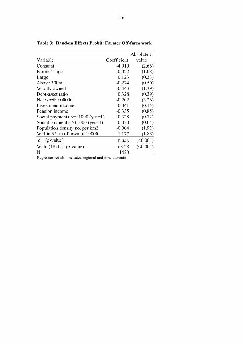
Table 3 reports the Random effects probit results, which represent the first stage

of the two-step estimation procedure. The vector of explanatory variables includes all the variables reflecting farm characteristics, non-farm income, and farm location reported in Table 1 plus regional and time dummies. The possibility that these variables are correlated with the random effect means that the estimates need to be interpreted with some caution. In particular, any estimated coefficient may reflect the relevant variable’s marginal effect plus its correlation with the random effect. Although the overall Wald test suggests that the explanatory variables are jointly significant (at less than 1 percent), few individual variables are statistically significant at 10 percent. Of these, the negative effect of Net worth and the positive effect of being within 15km of a town of 10000 are as one might expect. In contrast, the effect of population density is significant but negative.

Also at the bottom of the Table, the value of ρ̂ is reported. This may be

interpreted as the proportion of the variance unexplained by the explanatory variables

accounted for by variation between individuals, i.e. 22

2

ηθ

θ

σσσ+

ρ = . The p-value

reported below ρ̂ tests the significance of this coefficient. Hence, the significant value reported indicates that taking account of unobserved heterogeneity is important.

Table 4 reports the results of the second step of the estimation procedure. Hence,

these regressions include the estimates of the two sample selection terms as explanatory variables (the bracketed terms in equations (4) and (5)). As discussed above, the coefficients on these two terms are estimates of the covariances between the random effects, αθσ , and between the random shocks, ησ e . These estimates are reported at the bottom of the Table. All the standard errors reported are based on a covariance matrix adjusted for the two-step nature of the estimation process and robust to autocorrelation and heteroskedasicity (Vella and Verbeek; Newey). For each production ratio used as a dependent variable, two sets of regression results are reported. As for the fixed effect regressions in Table 2, one of these uses other information on the farm, i.e. dummies reflecting larger farms, the farm’s altitude and ownership status, plus regional and time dummies. To explore whether the endogeneity of these variables is a particular problem, a restricted regression is also reported, where only the off-farm work variables plus the regional and time dummies are included as regressors.

The results provide some evidence that the selection model is necessary and that

the off-farm work decision is endogenous to production decisions. For example, the

9

estimate of the covariance αθσ̂ is significant (at 10 percent) in the equations explaining log(output per hectare) and the proportion of output from livestock, while the estimate of the covariance ησ eˆ is significant (at 10 percent) in the equations explaining the proportion of output from crops and from milk.

In terms of the effect of off-farm work, the results are qualitatively similar to

the fixed effects results, namely, there is some evidence that the farmer’s off-farm work decision affects current inputs per hectare and the proportion of output from crops and milk, while there is little evidence that the off-farm work decision of the spouse has any significant impact on the production ratios or the enterprise mix (the only exception to this is the impact of spouse off-farm work on the proportion of output from milk in the restricted regression results). However, the estimates of these effects are considerably greater than those reported in Table 2. For example, in the restricted regression results a farmer’s off-farm work decisions leads to a 26 percent reduction in the use of current inputs, a 10 point increase in the proportion of output from crops and a 13 point reduction in the proportion of output from milk. In contrast to the fixed effects model results, there no evidence from Table 4 that farmer’s off-farm work has a significant impact on the proportion of output from livestock. Summary and Conclusions This paper has considered the effect of off-farm work on input and output intensities and on the structure of farm output using farm level panel data. Specifically, we estimate the impact of off-farm work on a number of output and input ratios using a sample selection model that accounts for both unobserved heterogeneity and the potential simultaneity between farm production and the farmer’s off-farm work decision. The results provide strong evidence to suggest that for the farmer at least, off-farm work does affect production and enterprise mix. Hence, farmer off-farm employment cannot simply be considered a residual activity after production decisions have been made. There is also some evidence that off-farm labour decisions and farm production decisions are simultaneous. In contrast, the results suggest that the off-farm work decision of the spouse has no effect on on-farm decisions.

The results also provide a number of research directions and questions for future work. For example, there is evidence of simultaneity in the output per hectare ratio and the off-farm labour decision but the evidence that off-farm work significantly affects the log(output per hectare) is rather weak. This appears difficult to reconcile with the evidence that, while current inputs per hectare are reduced significantly by the farmer’s off-farm work they do not appear simultaneous with the off-farm labour decision. One possible explanation, which could be further explored, is that these differences arise from the effect of restrictions on off-farm hours.

More generally, the panel sample selection model used here would appear to have

potential for wider application. In particular, where theory suggests that a farm household approach should form the basis of empirical work, the model’s ability to control for unobserved heterogeneity in both production and off-farm decisions appears extremely useful in a range of situations where data is limited.

10

References Arulampalam , W, A. Booth, and M. Taylor. ‘Unemployment persistence’ Oxford

Econ. Paper. 52 : 24-54. January 2000. Blundell R, Bond S ‘Initial conditions and moment restrictions in dynamic panel data

models’ J Econometrics, 87 (1): 115-143 November 1998. Baltagi B Econometric Analysis of Panel Data NewYork: John Wiley 2002. Bewley R and Young T ‘Applying Theil multinomial extension of the linear logit

model to meat expenditure data’ Am J Agr Econ 69 (1): 151-157 February 1987.

Blandford D and Boisvert R N Non-trade concerns and Domestic/International Policy Choice International Agricultural Trade Research Consortium Working Paper 02-1. 2002.

Bokemeier J and Garkovitch L ‘Assessing the influence of farm womens' self-identity on task allocation and decision-making’, Rural Sociol, 52 (1): 13-36 Spring 1987.

Carlin T and Bentley S ‘Modelling On-farm adjustments’ in Multiple job-holding among farm families. (Eds. Halberg, M.C., Findeis, J.L. and Lass, D.A.) Iowa State University Press, Ames. Iowa 1991.

Chamberlain, G. “Panel Data”. Handbook of Econometrics Vol 2.. Z.Griliches and M. Intriligator eds., pp.1247-1318. NewYork: North Holland. 1984.

Constadine, T and Mount T ‘The use of linear of linear logit-models for dynamic input demand systems’ Rev Econ Stat 66 (3): 434-443 1984.

Cooper J and Keim R ‘Incentive payments to encourage farmer adoption of water quality protection practices’ Am J Agr Econ 78 (1): 54-64 February 1996.

Coughenour C, Swanson L ‘Work statuses and occupations of men and women in farm families and the structure of farms’, Rural Sociol 48 (1): 23-43 1983.

Ellis N.E., Heal O.W., Dent J.B. and Firbank L.G. ‘Pluriactivity, farm household socio-economics and the botanical characteristics of grass fields in the Grampian region of Scotland’. Agric Ecosystems Environ 76(2-3), 121-134. 1999.

EU Commission “Safeguarding the multifunctional role of EU agriculture: which instruments”. Info Paper Brussels. EC Commission. 1999

EU Commission “Agriculture’s contribution to rural development”. Conference Paper Non-Trade Concerns in Agriculture. Ullensvang, Norway, 2-4-July 2000.

Fuglie K and Bosch D ‘Economic and environmental implications of soil-nitrogen testing - a switching-regression analysis’ Am J Agr Econ 77 (4): 891-900 November 1995.

Gasson R. Part-time Farming and Pluriactivity, In: Britton D (ed.) Agriculture in Britain: Changing Pressures and Policies, Wallington, England: CAB International. 1990.

Greene, W. Econometric Analysis. New York, Prentice Hall. 1993. Heckman JJ, Snyder JM ‘Linear probability models of the demand for attributes with

an empirical application to estimating the preferences of legislators’ Rand J Econ 28: S142-S189 1997.

Hill B. Farm Incomes, Wealth and Agricultural Policy. 3rd Edition. Ashgrove: Ashgate. 2000.

Huffman, W.E “Agricultural Household Models: Survey and Critique” Multiple Job Holding among Farm Families. A.O. Lass, , L.J. Findeis and M.C Halberg eds., pp.239-262. Ames: Iowa State University Press 1991.

11

Hyslop, D.R. “State dependence, serial correlation and heterogeneity in intertemporal labour force participation of married women”, Econometrica 67 1255-1294 November 1999.

Khanna, M ‘Sequential adoption of site-specific technologies and its implications for nitrogen productivity: A double selectivity model’ Am J Agr Econ 83 (1): 35-51 February 2001.

Lass D.A., Findeis J.L. and Hallberg M.C. Factors affecting the supply of off-farm labour: A review of empirical evidence. In Multiple job-holding among farm families. (Eds. Halberg, M.C., Findeis, J.L. and Lass, D.A.) Iowa State University Press, Ames. Iowa 1991.

Lindland J. Non-trade concerns in a Multifunctional Agriculture: Implications for Agricultural Policy and the Multilateral trading System. Paris. OECD 1998

Lopez RE ‘Estimating labour supply and production decisions of self-employed farm producers’ Eur Econ Rev 24 (1). 61-82 1984.

Nakajima C Subjective Equilibrium Theory of the Farm Household. Amsterdam Elsevier.

Newey, W. A method of moments interpretation of sequential estimators. Econ Lett 14, 201-206. 1984.

Nijman, T., Verbeek, M., Nonresponse in panel data: The impact on estimates of a life cycle consumption function. Journal of Applied Econometrics 7, 243-157. 1992.

Olfert, R ‘Nonfarm, employment as a response to underemployment in agriculture’ Can J Agr Econ 40: 443-458 1992.

Olfert, R ‘Off-farm Labour Supply with Productivity Increases, Peak Period Production and Farm Structure Impacts’, Can J Agr Econ 41 491-501 1993.

Rosegrant MW, Kasryno F, Perez ND ‘Output response to prices and public investment in agriculture: Indonesian food crops’ J Dev Econ 55 (2): 333-352 April 1998.

Shucksmith M and Smith R Farm household strategies and pluriactivity in upland Scotland, J Agr Econ 42 (3): 340-353 September 1991.

Vella, F, Verbeek, M. ‘Two-step estimation of panel data models with censored endogenous variables and selection bias’. J Econometrics, 90 239-263.1999.

Verbeek, M and Nijman T ‘Testing for selectivity bias in panel data models’, Int Econ Rev, 33. 1992.

Weiss CR ‘Farm growth and survival: Econometric evidence for individual farms in Upper Austria’ Am J Agr Econ 81 (1): 103-116 February 1999.

Willock J, Deary IJ, Edwards-Jones G, Gibson GJ, McGregor MJ, Sutherland A, Dent JB, Morgan O, Grieve R ‘The role of attitudes and objectives in farmer decision making: Business and environmentally-oriented behaviour in Scotland’ J Agr Econ 50 (2): 286-303 May 1999.

Wu JJ, Babcock BA ‘The choice of tillage, rotation, and soil testing practices: Economic and environmental implications’ Am J Agr Econ 80 (3): 494-511 August 1998.

12

Appendix Data Construction and Definitions Large farms –defined as those equal or greater than 100 Economic Size Units (ESU) where each unit is equivalent to 1200 standard gross margins. These latter values are financial measures based on gross margins and are used to classify farms by size and type. Holdings of less than 8 ESU are considered too small to provide full-time work for one person. Owner-occupied: The Area Used for Agriculture wholly owned and farmed by the occupier directly, through a paid manager or a contract farming agreement. Above 300m: Most of the holding above 300 metres. Debt-asset ratio: (Total business liabilities at opening valuation)/(total business liabilities+ net worth opening valuation). Net worth: Net worth opening valuation. Investment Income: Income from interest on personal bank, building society and similar accounts. Also included is income from dividends on shares not associated with the farm business, rental income from property off the farm, income in “non-cash form . Pension Income: Income from occupational and state pension schemes, including retirement, widows and disability pensions. Social payments: Income from sources such as child benefit, family credit or other cash welfare payments. Population density: Measured as population per kilometre squared using district level data on population and area drawn from 1991 UK Census. Within 35km of town of 10000:The distance was measured from an area of population 10000 + (1991 census) to the farms (10km Grid Square), using the road network. As the exact location of the farm within each 10km square was unknown, it was assumed the farm could be anywhere within the square. Total farm output was disaggregated into the following components; total crop output, livestock output, milk, other produce and miscellaneous output. Each component was deflated by the appropriate UK index of Producer Prices using 1998 as the base year to generate the real value Where no specific index existed, e.g. miscellaneous output, the general UK index of Producer Prices for all Agricultural Products was applied. Total Current Inputs were defined as expenditure on fuel and electricity, miscellaneous inputs, crop protection, other crop expenses, fertilisers, seeds, other livestock expenses plus feed. As for output each component was deflated by the appropriate UK index of Input Prices using 1998 as the base year. Where no specific index existed, the general UK index of general agricultural expenses was applied.

13

Figure 1: Variable Off-farm Hours Consumption/Output U B

b a AU T Leisure Figure 2: Fixed Off-farm Hours Consumption Output U B

b a AU T Leisure

14

Table 1: Descriptive Statistics

All Farms Off-farm work Farmer Spouse

Production Structure Output per hectare* 772.4 627.0 705.1Total Current Inputs per hectare** 312.6 231.7 282.9Proportion Output from Crops 0.216 0.258 0.228Proportion Output from Livestock 0.598 0.635 0.625Proportion Output from Milk Products 0.122 0.026 0.071Farm Characteristics Farmer’s Age 53.9 52.4 49.4Large Farm 0.213 0.162 0.142Above 300m 0.102 0.106 0.122Wholly Owned 0.493 0.373 0.474Debt-asset ratio 0.163 0.175 0.212Net worth £00000 4.429 3.416 3.578Non-farm Income Investment Income 0.325 0.366 0.293Pension Income 0.104 0.077 0.034Social payments <=£1000 0.093 0.085 0.169Social payment s >£1000 0.127 0.169 0.186Farm Location Population density No per km2 68.9 39.8 51.1Within 35km of town of 10000 0.810 0.789 0.731Central Region 0.205 0.176 0.208Northern isles 0.071 0.113 0.115Highland 0.141 0.120 0.147Grampian 0.230 0.176 0.237South 0.354 0.415 0.293Year 1998 0.318 0.282 0.2371999 0.349 0.345 0.3642000 0.333 0.373 0.399Number of Observations 1420 142 409 *Output and Total Current Inputs per hectare are real 1998 constant values. **All per hectare ratios are calculated relative to the total agricultural area of the farm

15

Table 2: On Farm Effects of Off-farm Work: Fixed Effects Estimates Dependent Variable

Log(Output/ha)

Log(Current Inputs/ha)

Proportion Output: Crops

Proportion Output: Livestock

Proportion Output: Milk

Farmer Off-farm Work -0.026 -0.065 0.016 0.016 -0.025 (0.9) (2.32) (2.11) (1.54) (3.98)Spouse Off-farm Work -0.005 -0.012 -0.002 0.004 0.000 (0.24) (0.55) (0.38) (0.55) (0.06)Large Farm 0.088 0.119 0.017 -0.005 0.000 (1.93) (2.67) (1.4) (0.33) (0.04)Wholly Owned 0.078 0.081 -0.006 0.006 -0.002 (2.83) (2.99) (0.75) (0.62) (0.4)

2R 0.061 0.055 0.008 0.002 0.05N 1420 1420 142 1420 14200Absolute t values in brackets. All Regressions also included time dummies.

16

Table 3: Random Effects Probit: Farmer Off-farm work

Variable CoefficientAbsolute t-

value Constant -4.010 (2.66)Farmer‘s age -0.022 (1.08)Large 0.123 (0.33)Above 300m -0.274 (0.50)Wholly owned -0.443 (1.39)Debt-asset ratio 0.328 (0.39)Net worth £00000 -0.202 (3.26)Investment income -0.041 (0.15)Pension income -0.335 (0.85)Social payments <=£1000 (yes=1) -0.328 (0.72)Social payment s >£1000 (yes=1) -0.020 (0.04)Population density no. per km2 -0.004 (1.92)Within 35km of town of 10000 1.177 (1.88)ρ̂ (p-value) 0.946 (<0.001)Wald (18 d.f.) (p-value) 68.28 (<0.001)N 1420Regressor set also included regional and time dummies.

Table 4: On Farm Effects of Off-farm Work: Sample Selection Model Dependent Variable

Log(Output/ha)

Log(Current Inputs/ha)

Proportion Output: Crops

Proportion Output: Livestock

Proportion Output: Milk

Constant

6.406 6.632 5.424 5.655 0.370 0.385 0.465 0.390 0.072 0.148(73.5) (72.3) (58.2) (59.0) (10.0) (10.7) (12.3) (11.0) (2.50) (5.30)

Farmer Off-farm Work

-0.097 -0.156 -0.176 -0.236 0.102 0.099 -0.020 -0.001 -0.109 -0.128(0.91) (1.30) (1.63) (1.93) (2.36) (2.25) (0.37) (0.01) (4.57) (5.05)

Spouse Off-farm Work

0.039 -0.046 0.044 -0.037 0.025 0.011 -0.004 0.024 -0.032 -0.049(0.54) (0.56) (0.57) (0.43) (1.22) (0.52) (0.17) (0.86) (1.62) (2.41)

Large Farm

0.447 0.418 0.092 -0.185 0.132 (4.79) (4.28) (3.33) (5.75) (4.10)

Above 300m

-1.203 -1.174 -0.152 0.328 -0.148 (7.87) (7.34) (7.36) (11.2) (6.39)

Wholly Owned

0.318 0.332 0.004 -0.084 0.086 (4.58) (4.47) (0.21) (3.30) (4.19)

αθσ̂ 1.736 2.049 0.977 1.300 0.333 0.344 -0.478 -0.552 0.023 0.083 (2.12) (2.32) (1.16 (1.44) (1.35) (1.44) (1.85) (1.91) (0.12) (0.34)

ησ eˆ 0.008 0.015 0.012 0.020 -0.009 -0.009 0.003 0.002 0.010 0.012 (0.64) (1.08) (0.98) (1.40) (1.91) (1.86) (0.57) (0.24) (3.04) (3.66)Absolute t values in brackets. Standard Errors are adjusted for two step estimation and are robust to heteroskedasticity and autocorrelation. All Regressions also included regional and time dummies.

18