The Effect of Modeling and Visualization Resources on ... · The Effect of Modeling and Visualization Resources on Student Understanding of Physical Hydrology Jill A. Marshall,1,a

The Effect of Modeling and Visualization Resources on StudentUnderstanding of Physical Hydrology

Jill A. Marshall,1,a Adam J. Castillo,1 and M. Bayani Cardenas2

ABSTRACTWe investigated the effect of modeling and visualization resources on upper-division, undergraduate and graduate students’performance on an open-ended assessment of their understanding of physical hydrology. The students were enrolled in oneof five sections of a physical hydrology course. In two of the sections, students completed homework problems and projectsusing only Excel (Microsoft, Redmond, WA) or MATLAB (MathWorks, Natick, MA) as modeling resources, and in the otherthree sections, some of the homework exercises were replaced with modeling and visualization activities using the interactivemodeling software COMSOL Multiphysics (COMSOL, Burlington, MA). Other aspects of the course (instructor, syllabuscoverage, lectures, and textbook) remained the same throughout the study. We performed a repeated-measures analysis ofvariance, which showed that gains from pretest to posttest were statistically significant overall and were independent of thesection in which students were enrolled for all but one component on the assessment. In that case, students who did not haveaccess to the COMSOL modules marginally outperformed the others, but not to the required level of statistical significance.These results were complemented by a qualitative investigation of students’ interaction with the modeling software. Weinterviewed a subset of students and assigned codes to themes that arose when we analyzed the resulting transcripts. Thisprocess allowed us to develop a theory of how students were interacting with the modeling and visualization resources. Asignificant theme was the issue of ‘‘scaffolding,’’ or supports, with both positive and negative consequences for students,depending on their personal preferences and previous experience. � 2015 National Association of Geoscience Teachers. [DOI:10.5408/14-057.1]

Key words: hydrology, physics, modeling, COMSOL

INTRODUCTIONNeed for Modeling and Visualization in PhysicalHydrology

In their call to action, Wagener et al. (2010) describedthe enormous challenges facing hydrologic research andeducation today and the ‘‘unprecedented opportunity’’ touse advances in modeling and visualization, which are‘‘prerequisites for detecting, interpreting, predicting andmanaging evolving hydrologic systems,’’ (p. 8) to addressthem. Merwade and Ruddell (2012) clearly articulated theimplications of modeling and visualization in hydrologyeducation:

‘‘Considering the extensive use of authentic data, integratedmodeling, and geospatial visualization in research applica-tions and in the professional world, training in theseapproaches is becoming necessary for a successful career inhydrology. For this reason alone, it seems reasonable tosuggest a strategy of supplementing the traditional hydrologycurriculum with the latest data and modeling approaches.’’(Merwade and Waddell, 2012, p. 2398).

In alignment with these calls for incorporation of datamodeling and visualization into hydrology instruction

(Wagener et al., 2012), faculty at the authors’ institutionhave developed a series of COMSOL Multiphysics3 (COM-SOL, Burlington, MA; Zimmerman, 2006) models ofhydrological systems, which permit students to visualize,explore, analyze, and predict the consequences of changes toa hydrologic system and its inputs. These modules comple-ment lecture-based instruction and other tools for datamodeling and manipulation, e.g., spreadsheet software, suchas Excel (Microsoft, Redmond, WA) and open-endedprogramming, and computational environments such asMATLAB (on which COMSOL was originally based; Math-Works, Natick, MA).

During the past five years, the modules have beenimplemented in a colisted, upper-division, undergraduate-and graduate-level physical hydrology course. The goals ofthis course are for students to (1) develop a quantitative,process-based understanding of hydrologic processes; (2)gain experience with different methods in hydrology; and (3)enhance their learning, problem-solving, and communica-tions skills. Developing an ‘‘. . . awareness of the totality ofinterconnected (mainly physical) processes involved in thehydrological cycle’’ (Nash et al., 1990, p. 606) has beenidentified as first among the goals of hydrology education,and there is increasing recognition that geoscience educationrequires a quantitative focus (Manduca et al., 2008). Thehydrology community also acknowledges the need toconnect this quantitative, theoretical understanding withknowledge of the methods and practices within the field(Wagener et al, 2012). The contents of the course in thisstudy matched quite well to those of the largest subset of

Received 1 October 2014; revised 4 February 2015; accepted 8 March 2015;published online 13 May 2015.1Department of Curriculum and Instruction, University of Texas, Austin,Texas 78712, USA2Department of Geological Sciences, University of Texas, Austin, Texas78712, USAaAuthor to whom correspondence should be addressed. Electronic mail:[email protected]. Tel.: 512-232-9685. Fax: 512-471-8460. 3 See http://www.comsol.com.

JOURNAL OF GEOSCIENCE EDUCATION 63, 127–139 (2015)

1089-9995/2015/63(2)/127/13 Q Nat. Assoc. Geosci. Teachers127

hydrology courses, i.e., civil engineering hydrology andgroundwater hydrology, in a study from several decades ago(Groves and Moody, 1992). Thus, the hydrology-specificgoals of the course aligned with those identified by thebroader community, and the course cannot be consideredatypical in that regard. What distinguishes this course is thedevelopment and addition of the COMSOL Multiphysicsmodeling and visualization modules to the curriculum. Thehomework exercises involving these modules are docu-mented in the online supplemental materials.4 The syllabusfor the course is also included in the online supplementalmaterials.5

To test the efficacy of the curriculum modules in meetingthe stated learning goals, the authors developed an open-ended assessment of student understanding of physicalhydrology (Marshall et al., 2013). The assessment consistedof three questions, mirroring course goals. The first askedstudents to describe the important physical processes inhydrology and how they affect hydrological systems, thesecond asked students to describe the relevant physical lawsthat govern hydrology and how they relate to hydrologicalprocesses, and the third asked students how they wouldassess the effects of a drought and urbanization on a localspring and to predict what the effects would be in the future.

Regarding the first question, important components ofthe water cycle are precipitation, runoff, evaporation, andtranspiration, which are also related to solar radiation andsoil-and-groundwater flow (or infiltration). In colder areas,snowfall and snow melting, sublimation, or evaporationwould be included. Precipitation is any moisture input fromthe atmosphere to the land, including both rainfall andsnowfall. Evaporation and transpiration comprise themoisture return to the atmosphere, which requires an inputof energy, coupling the water cycle to the energy cycle.Transpiration is moisture uptake by plants from roots andreleased to the atmosphere. Soil-and-groundwater flow isthe redistribution of water underground, which is due togravity, pressure, and capillary forces.

Regarding the second question, the relevant physicallaws that govern hydrology are the conservation laws ofmass and energy and the conservation of momentum.Fundamentally, these are the laws of thermodynamics andNewton’s second law. There are multiple forms of theequation showing Flux = (Resistance or conductance coefficient)· Gradient. Examples of this include Darcy’s law forgroundwater flow in saturated porous media or the Richardsequation for unsaturated flow of moisture through soils,equations for mass and energy transfer or evaporation andtranspiration from soil and water surfaces, Manning’sequation for open channel flow, Fick’s law for solutediffusion, and Fourier’s law for heat transfer.

For the third question, to predict the effects of continueddrought and urbanization, a hydrologist would collecthistorical data, especially during nondrought years andbefore urbanization, then continue to monitor for the sameinformation. These data would primarily include rainfall andspring discharge and, perhaps, water quality. Based on thehistorical data, either a statistical model or a process-basedmodel (e.g., a groundwater flow model) would need to be

built, calibrated to the historical data. Urbanization can berepresented by the amount of impervious cover from mapsor population data (but that isn’t really hydrology). Once amodel is calibrated, it can be used to analyze what mighthappen under different forcing conditions that are notrepresented in the data, such as extreme and prolongeddrought or continued growth of the city.

This article reports results of a 3-y study to compareprecourse and postcourse responses of students (bothgraduate and upper division undergraduate) in the physicalhydrology course. Depending on the semester in which theytook the course, students were tasked with modelinghydrologic phenomena using either Excel and/or MATLABalone or with the application of COMSOL Multiphysics aspart of the assigned homework. During the course of thestudy, the instructor remained the same, and other aspects ofthe course (lecture, exams, student projects, and presenta-tions, etc.) were deliberately held as constant as possible.Examination of course grades and pretest scores indicated nosystematic variation in the student population over this time;however, possible unidentified variation in the populationconstitutes a limitation of the study.

Specifically, we sought to determine

� How do different modeling utilities compare in termsof enhancing student mastery of course goals asassessed by before and after tests?

� How do students describe their interactions/experi-ences with different approaches to modeling andvisualization?

STUDY DESCRIPTIONSetting

The study took place in five sections of a colisted, upper-division, undergraduate and graduate, physical hydrologyclass, offered in a department of geological sciences, over thecourse of 3 y. Each of the sections was taught by the sameinstructor, one of the authors (M.B.C.). The class is based on,and closely follows, the textbook Physical Hydrology by S. L.Dingman (2008), a later edition of the most often usedtextbook cited by Wagener et al. (2007). The semester-longclass is targeted toward upper-division, undergraduatestudents and new graduate students studying hydrology orhydrogeology. The class covered the following broad topics,which included all aspects of the hydrologic cycle: (1)atmospheric and climate processes; rainfall; (2) snow andsnowmelt; (3) unsaturated zone and infiltration processes;(4) evaporation and transpiration; (5) runoff processes,streamflow, and watershed hydrology; and (5) groundwaterhydrology. Roughly 2 to 3 weeks are devoted to each topic.(A sample syllabus is included in the online supplementarymaterials5).

The topics are presented such that a molecule of water isessentially tracked through the hydrologic cycle, beginningin the atmosphere, where it condenses to form rainfall orsnow, then as rain and snow (with snow potentiallyaccumulating on the ground), with some water going backto the atmosphere (evaporation and transpiration). Infiltra-tion across the soil surface and soil moisture flow are thendiscussed, with water that did not infiltrate becoming runoffon the land surface and eventually forming streamflow.Finally, water that infiltrated through the unsaturated soil

4 The homework exercises can be found online at http://dx.doi.org/10.5408/14-057s1.5 The syllabus can be found online at http://dx.doi.org/10.5408/14-057s2.

128 Marshall et al. J. Geosci. Educ. 63, 127–139 (2015)

reaches the water table of aquifers. At this point, ground-water hydrology is covered, the last topic of the class. Ateach step, the pertinent physics, and to a certain extent,thermodynamics, are taught.

The class grading is heavily weighted toward assign-ments, with homework comprising 50% of the final grade.One homework assignment is assigned approximately everytwo weeks with a total of six homework assignmentsthroughout the duration of the semester. The modelingand visualization activities, discussed in detail below, wereintegrated into the third and sixth (final) homeworkassignments (see online supplemental materials4), whenthe instructor felt that modeling and visualization wouldparticularly help in the students’ learning and appreciationof the topic.

ParticipantsIn all, 80 participants, out of a total enrollment of 95,

consented to participate. We were able to match preassess-ment and postassessment scores for 51 students. Somestudents completed only the pretest (and were not presentfor the posttest or had dropped the course), and others werenot present at the beginning of class on the first day andcompleted only the posttest or did not label their assess-ments in such a way that they could be matched.Assessments that could not be matched were used forsummary statistics only. Additionally, 14 students consentedto be interviewed. Because not every student consented toparticipate and completed both the pretest and posttest andthe numbers of participants were too small to disaggregatethe data by gender or student status, there is a limitation onthe generalizability of the study results.

The participants were either upper-division, undergrad-uate or graduate students enrolled in a section of a physicalhydrology course, cross-listed as undergraduate/graduateand offered in the geological sciences, over a 3-y period. Thecourse is a requirement for undergraduate students majoringin geology with a hydrogeology emphasis or geosystemsengineering and hydrogeology (a hybrid program betweenpetroleum engineering and hydrogeology) and is an electivefor general geology and environmental science students.Calculus and a previous introductory hydrogeology courseare prerequisites. Graduate students taking the course mightbe from the geosciences or engineering, occasionally otherareas, and for them, there were no prerequisites, andenrollment was based on instructor consent. The differencein prerequisites for the undergraduate and graduate versionsof the course tended to yield overlapping distributions interms of preparation, particularly mathematical preparation,for the undergraduate and graduate students. In otherwords, graduate students were not, on average, likely to bebetter prepared technically than undergraduates in terms ofphysical hydrology.

Modeling and Visualization ResourcesDuring the first year (two sections of the course),

students were required to use Excel spreadsheets orMATLAB to manipulate data and produce graphs/plotsthrough which trends in hydrologic interactions could bevisualized and analyzed. Arguably, Excel presents only thecrudest modeling capability, but using it, students might, forexample, plot the Darcy flux (described below) versus headgradient by entering the equation corresponding to Darcy’s

Law into Excel. They could then identify trends from theresulting graph of pressure versus output flow, arguablyperforming rudimentary modeling and analysis.

During the second 2 y (three sections of the course),students were given access to, and required to use,COMSOL Multiphysics to model some of the same hydro-geological phenomena. COMSOL Multiphysics is a generic,finite-element, numerical modeling software. Its origin canbe traced back to the partial-differential equation numericalsolver toolbox for MATLAB, which then evolved intoindependent modeling software with a user-friendly, Win-dows-based, graphical user interface. The COMSOL Multi-physics user interface integrates all modeling aspects, fromchoosing which governing differential (conservation) equa-tions to solve, setting boundary conditions and internaldomain parameters or coefficients, building structured orunstructured finite-element meshes, to postprocessing andvisualization of results, including generation and viewing ofanimations. The workflow from model conceptualization,domain and geometry setup, finite-element mesh genera-tion, solution (or actual model run) to postprocessing is alltightly integrated and sequentially arranged.

The assigned homework problems that use COMSOLare included as part of the online supplemental materials.4

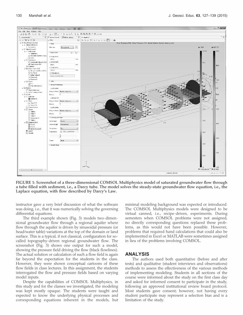
Figure 1 shows screenshots from a COMSOL Multiphysicsexercise modeling a Darcy tube and allows students todiscover Darcy’s Law for themselves. The model shown wascreated for students using COMSOL Multiphysics, andstudents were asked to modify the inputs and interrogate theresults, i.e., a rudimentary sensitivity analysis. Figure 1 alsoillustrates the COMSOL Multiphysics workflow (left side ofthe screenshot); the user would have to go sequentiallythrough all the tabs from top to bottom, but in this case,these have already been prepopulated. This example showsgroundwater flow through a tube packed with sand, i.e., aDarcy tube. Darcy’s law—the fundamental equation de-scribing fluid flow through porous media—was empiricallyderived through experiments by Henry Darcy with thesetubes. The students were essentially made to replicateDarcy’s experiments computationally and digitally usingCOMSOL Multiphysics. In Fig. 1, water is injected from theleft into the tube and comes out on the right end (arrowsindicate the flow). The flow is driven by a linear pressuredrop; the pressure field is indicated by shading in the circularcross sections.

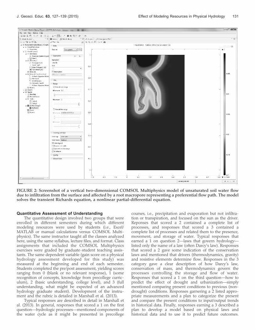
Figures 2 and 3 illustrate two other examples of assignedproblems that use COMSOL Multiphysics. Figure 2 shows ascreenshot of a model for unsaturated flow through a two-dimensional vertical cross section of soil with a root servingas a macropore (i.e., a fast-flow path, or ‘‘wormhole’’). Itshows the saturation of the soil (1 being saturated) sometime after infiltration from the top started. This model solvesthe Richards equation, which is a nonlinear, partial-differential equation. The students were introduced to theequation in class lectures, but such a numerical modelsimulation using the Richards equation is far beyond whatthe class would normally cover. For example, writing theirown programs to solve this would require many semesters ofcourses in mathematical modeling. The idea of this exercise,as with other COMSOL Multiphysics problems, is toinvestigate how the system works when certain parametersare changed. The modeling aspects, for the most part,remained as a black box for the students, although the

J. Geosci. Educ. 63, 127–139 (2015) Effect of Modeling Resources in Physical Hydrology 129

instructor gave a very brief discussion of what the softwarewas doing, i.e., that it was numerically solving the governingdifferential equations.

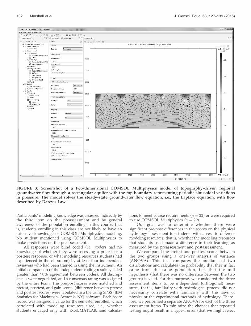
The third example shown (Fig. 3) models two-dimen-sional groundwater flow through a regional aquifer whereflow through the aquifer is driven by sinusoidal pressure (orhead/water table) variations at the top of the domain or landsurface. This is a typical, if not classical, configuration for so-called topography-driven regional groundwater flow. Thescreenshot (Fig. 3) shows one output for such a model,showing the pressure field driving the flow (black flowlines).The actual solution or calculation of such a flow field is againfar beyond the expectation for the students in the class.However, they were shown conceptual cartoons of theseflow fields in class lectures. In this assignment, the studentsinterrogated the flow and pressure fields based on varyingmodel inputs.

Despite the capabilities of COMSOL Multiphysics, inthis study and for the classes we investigated, the modelingwas kept mostly opaque. The students were taught andexpected to know the underlying physical processes andcorresponding equations inherent in the models, but

minimal modeling background was expected or introduced.The COMSOL Multiphysics models were designed to bevirtual canned, i.e., recipe-driven, experiments. Duringsemesters when COMSOL problems were not assigned,no directly corresponding questions replaced these prob-lems, as this would not have been possible. However,problems that required hand calculations that could also beimplemented in Excel or MATLAB were sometimes assignedin lieu of the problems involving COMSOL.

ANALYSISThe authors used both quantitative (before and after

tests) and qualitative (student interviews and observations)methods to assess the effectiveness of the various methodsof implementing modeling. Students in all sections of thecourse were informed about the study on the first class dayand asked for informed consent to participate in the study,following an approved institutional review board protocol.Most students gave consent; however, not having everystudent participate may represent a selection bias and is alimitation of the study.

FIGURE 1: Screenshot of a three-dimensional COMSOL Multiphysics model of saturated groundwater flow througha tube filled with sediment, i.e., a Darcy tube. The model solves the steady-state groundwater flow equation, i.e., theLaplace equation, with flow described by Darcy’s Law.


Quantitative Assessment of UnderstandingThe quantitative design involved two groups that were

enrolled in different semesters during which differentmodeling resources were used by students (i.e., Excel/MATLAB or manual calculations versus COMSOL Multi-physics). The same instructor taught all the classes analyzedhere, using the same syllabus, lecture files, and format. Classassignments that included the COMSOL Multiphysicsexercises were graded by graduate-student teaching assis-tants. The same dependent variable (gain score on a physicalhydrology assessment developed for this study) wasmeasured at the beginning and end of each semester.Students completed the pre/post assessment, yielding scoresranging from 0 (blank or no relevant response), 1 (somerecognition of concepts, knowledge from precollege curric-ulum), 2 (basic understanding, college level), and 3 (fullunderstanding, what might be expected of an advancedhydrology graduate student). Development of the instru-ment and the rubric is detailed in Marshall et al. (2013).

Typical responses are described in detail in Marshall etal. (2013). In general, responses that scored a 1 on the firstquestion—hydrologic processes—mentioned components ofthe water cycle as it might be presented in precollege

courses, i.e., precipitation and evaporation but not infiltra-tion or transpiration, and focused on the sun as the driver.Reponses that scored a 2 contained a complete list ofprocesses, and responses that scored a 3 contained acomplete list of processes and related them to the presence,movement, and storage of water. Typical responses thatearned a 1 on question 2—laws that govern hydrology—listed only the name of a law (often Darcy’s law). Responsesthat scored a 2 gave some indication of the conservationlaws and mentioned that drivers (thermodynamics, gravity)and resistive elements determine flow. Responses in the 3category gave a clear description of how Darcy’s law,conservation of mass, and thermodynamics govern theprocesses controlling the storage and flow of water.Responses that scored a 1 on the third question—how topredict the effect of drought and urbanization—simplymentioned comparing present conditions to previous (non-drought) conditions. Responses garnering a 2 listed appro-priate measurements and a plan to categorize the presentand compare the present conditions to input/output trendsin historical data. Finally, responses earning a 3 described aplan to develop a model based on physical laws andhistorical data and to use it to predict future outcomes.

FIGURE 2: Screenshot of a vertical two-dimensional COMSOL Multiphysics model of unsaturated soil water flowdue to infiltration from the surface and affected by a root macropore representing a preferential flow path. The modelsolves the transient Richards equation, a nonlinear partial-differential equation.


Participants’ modeling knowledge was assessed indirectly bythe third item on the preassessment and by generalawareness of the population enrolling in this course, thatis, students enrolling in this class are not likely to have anextensive knowledge of COMSOL Multiphysics modeling.No student mentioned using COMSOL Multiphysics tomake predictions on the preassessment.

All responses were blind coded (i.e., coders had noknowledge of whether they were assessing a pretest or aposttest response, or what modeling resources students hadexperienced in the classroom) by at least four independentreviewers who had been trained in using the instrument. Aninitial comparison of the independent coding results yieldedgreater than 90% agreement between coders. All discrep-ancies were negotiated, and a consensus rating was assignedby the entire team. The pre/post scores were matched andpretest, posttest, and gain scores (difference between pretestand posttest scores) were tabulated in a file using SPSS (IBMStatistics for Macintosh, Armonk, NY) software. Each scorerecord was assigned a value for the semester enrolled, whichcorrelated with modeling resources used, i.e., whetherstudents engaged only with Excel/MATLAB/hand calcula-

tions to meet course requirements (n = 22) or were requiredto use COMSOL Multiphysics (n = 29).

Our goal was to determine whether there weresignificant pre/post differences in the scores on the physicalhydrology assessment for students with access to differentmodeling resources, that is, whether the modeling resourcesthat students used made a difference in their learning, asmeasured by the preassessment and postassessment.

We compared the pretest and posttest scores betweenthe two groups using a one-way analysis of variance(ANOVA). This test compares the medians of twodistributions and calculates the probability that they in factcame from the same population, i.e., that the nullhypothesis (that there was no difference between the twogroups) is valid. For this purpose, we considered the threeassessment items to be independent (orthogonal) mea-sures; that is, familiarity with hydrological process did notnecessarily correlate with familiarity with the laws ofphysics or the experimental methods of hydrology. There-fore, we performed a separate ANOVA for each of the threeassessment items. To minimize the chances that repeatedtesting might result in a Type-I error (that we might reject

FIGURE 3: Screenshot of a two-dimensional COMSOL Multiphysics model of topography-driven regionalgroundwater flow through a rectangular aquifer with the top boundary representing periodic sinusoidal variationsin pressure. The model solves the steady-state groundwater flow equation, i.e., the Laplace equation, with flowdescribed by Darcy’s Law.


the null hypothesis even though there was in fact no truedifference between the groups), we required a more-stringent level significance, p < .01, as opposed to the p< 0.05 level typically accepted. (Note that a typicalapproach to the issue of repeated testing is to use theBonferroni correction, i.e., to divide the required signifi-cance level by the number of tests, in this case, three.)

In addition, because the number of subjects was smallfor the different groups, we were careful to check that ourdata met the requirements for ANOVA. For an ANOVA tobe valid, (1) there must be no outliers in either group, (2)each group’s data must be normally distributed. and (3) eachgroup must have equal variance (homogeneity of variances).

To test for outliers, we created box plots in SPSS, fromwhich we identified one gain score as an outlier. That scoreresulted from a case in which a student had a clear, well-articulated pretest but left portions of the posttest substan-tially blank, possibly due to time restrictions. This data pointwas eliminated from the set, leaving a total of 50 matchedpretest and posttest scores for further analysis.

Because our sample size was large enough, we usedgraphical methods to determine whether the data met thenormality assumption for ANOVA. The box plots used tocheck for outliers indicated a normal distribution of gainscores for each question, once the lone outlier was removed.We also created Q-Q plots (plot of expected versus observeddistribution of scores), and data values appeared to followthe 458 normal line; therefore, we judged that the dependentvariable was normally distributed for both groups.

Finally, we tested for homogeneity of variances in thegain scores because the one-way ANOVA assumes that thepopulation variances of the dependent variable are equal forall groups. If the variances are unequal, the Type-I error rateis affected. There was homogeneity of variances of the gainscores for the process assessment component (p = 0.63), thelaw assessment component (0.57), and the methodologyassessment component (p = 0.47), as assessed by Levene’stest of homogeneity of variance, meeting that requirement.

Qualitative Assessment of Interactions With ModelingResources

In addition to the statistical analysis of student learning,a volunteer sample of students were interviewed about theirexperiences in the course, in particular, their interactionswith whichever modeling and visualization resources theyhad been required to use during the semester. In all, 14students were interviewed, representing a sampling ofundergraduate and graduate students, male and femaleparticipants, and students enrolled in each of the sections.Interviews were recorded and transcribed. In addition,students were observed as they interacted with a teachingassistant for the course during help/study sessions for thecourse. All the resulting artifacts (interview transcriptionsand observation notes) were then independently open codedfor concepts related to modeling and visualization and fortheir interaction with learning and other aspects of thecourse (see, for example, Mann [1993] for an explanation ofthe coding process in grounded analysis). The interviewedstudents presented both positive and negative perspectiveson different aspects of the course, making it seem unlikelythat the students who were interviewed, albeit a volunteersample, presented a systematic bias.

The concepts identified in the open coding werecompared, common themes were identified, and commonterminology and coding schemes were negotiated. Inter-views were independently coded using this scheme, and asubset of the independently assigned codes were comparedyielding agreement at the 98–99% level. After all interviewshad been coded, a common categorization scheme for thecodes was developed by negotiation, and a theory ofstudent interaction with the visualization resources wasdeveloped.

QUANTITATIVE RESULTSAs a first step in comparing the results of the posttest to

those from the pretest, we created before and afterhistogram plots for each of the three components of theassessment in each semester. In comparing the frequencyhistograms for scores on each of the three assessmentquestions, a shift toward more positive scores from thepretest to posttest on each component of the assessment wasevident for each semester the course was taught, i.e., bothfor the students who used Excel/MATLAB (year 1) and forthose who used COMSOL (years 2 and 3). Figure 4 showsthe before histogram (top row) and after histogram (bottomrow) for each of the three assessment components forstudents who had access to COMSOL (white bars) andthose who did not (gray bars).

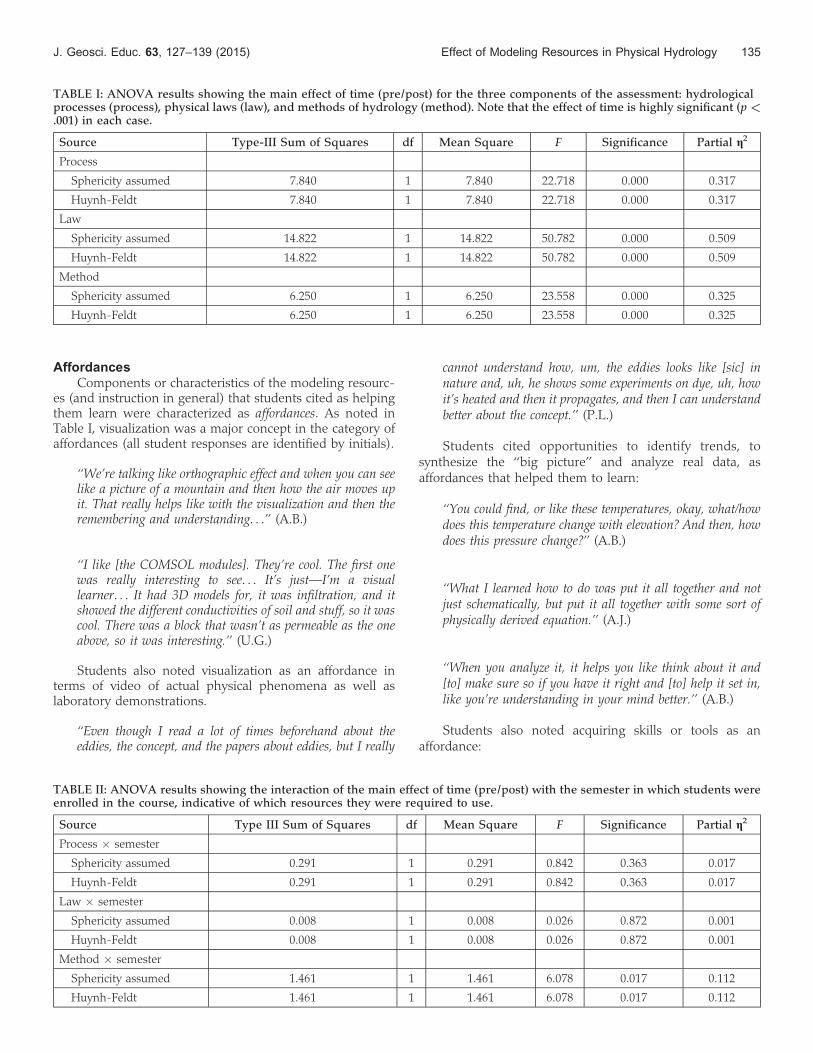
To test for the significance of this difference, weexamined the main effect of time using a repeated-measures(within-subjects) ANOVA, which compares the mean of thepretest scores to the mean of the posttest scores anddetermines the probability that the pretest and posttestresults might have come from the same distribution (i.e.,that there was no change in the scores from the pretest tothe posttest). Table I shows the results for the process, laws,and methodology questions, respectively. Each indicates adifference between pretest and posttest scores on all threequestions that is significant at the p < .001 level, meaningthat, overall, student scores improved from pretest toposttest. There was statistically significant learning in eachcase.

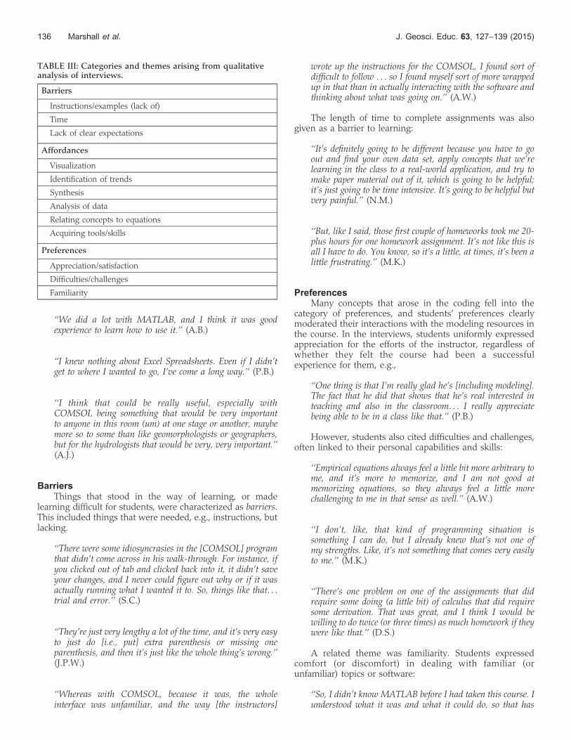
Table II shows the interaction between the semester astudent was enrolled in the course, indicative of themodeling and visualization resources that were available tohim or her, and the main effect of time (pre/post) on scoresfor each component of the assessment. There was nostatistically significant interaction between the semester astudent participated and the process component [F(1, 48) =0.84, p > 0.05] or the physical laws component of theassessment [F(1, 48) = 0.03, p > 0.05] meaning that pre-postdifference did not depend on the semester in which therespondent was enrolled, i.e., which modeling resourcesthey used, for these two questions.

The interaction between semester and the methodol-ogy component of the assessment, however, approachedsignificance [F(1, 48) = 6.08, p < 0.05 (but not <0.01)]leading us to investigate a possible difference on thiscomponent between the two groups. Inspection of themeans plots for the two groups shows that group that usedExcel, showed a larger improvement (mean = 0.77, SD =0.65) on the methodology component of the hydrologyassessment than the group that used COMSOL Multi-physics (mean = 0.29, SD = 0.73). Although this result is


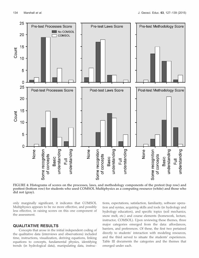
only marginally significant, it indicates that COMSOLMultiphysics appears to be no more effective, and possiblyless effective, in raising scores on this one component ofthe assessment.

QUALITATIVE RESULTSConcepts that arose in the initial independent coding of

the qualitative data (interviews and observations) includedtime, instructions, visualization, deriving equations, linkingequations to concepts, fundamental physics, identifyingtrends (in hydrological data), manipulating data, instruc-

tions, expectations, satisfaction, familiarity, software opera-

tion and syntax, acquiring skills and tools (in hydrology and

hydrology education), and specific topics (soil mechanics,

snow melt, etc.) and course elements (homework, lecture,

instructor, COMSOL). Upon reviewing these themes, three

major categories emerged from the data: affordances,

barriers, and preferences. Of these, the first two pertained

directly to students’ interaction with modeling resources,

and the third served to situate the students’ experiences.

Table III documents the categories and the themes that

emerged under each.

FIGURE 4: Histograms of scores on the processes, laws, and methodology components of the pretest (top row) andposttest (bottom row) for students who used COMSOL Multiphysics as a computing resource (white) and those whodid not (gray).


AffordancesComponents or characteristics of the modeling resourc-

es (and instruction in general) that students cited as helpingthem learn were characterized as affordances. As noted inTable I, visualization was a major concept in the category ofaffordances (all student responses are identified by initials).

‘‘We’re talking like orthographic effect and when you can seelike a picture of a mountain and then how the air moves upit. That really helps like with the visualization and then theremembering and understanding. . .’’ (A.B.)

‘‘I like [the COMSOL modules]. They’re cool. The first onewas really interesting to see. . . It’s just—I’m a visuallearner. . . It had 3D models for, it was infiltration, and itshowed the different conductivities of soil and stuff, so it wascool. There was a block that wasn’t as permeable as the oneabove, so it was interesting.’’ (U.G.)

Students also noted visualization as an affordance interms of video of actual physical phenomena as well aslaboratory demonstrations.

‘‘Even though I read a lot of times beforehand about theeddies, the concept, and the papers about eddies, but I really

cannot understand how, um, the eddies looks like [sic] innature and, uh, he shows some experiments on dye, uh, howit’s heated and then it propagates, and then I can understandbetter about the concept.’’ (P.L.)

Students cited opportunities to identify trends, tosynthesize the ‘‘big picture’’ and analyze real data, asaffordances that helped them to learn:

‘‘You could find, or like these temperatures, okay, what/howdoes this temperature change with elevation? And then, howdoes this pressure change?’’ (A.B.)

‘‘What I learned how to do was put it all together and notjust schematically, but put it all together with some sort ofphysically derived equation.’’ (A.J.)

‘‘When you analyze it, it helps you like think about it and[to] make sure so if you have it right and [to] help it set in,like you’re understanding in your mind better.’’ (A.B.)

Students also noted acquiring skills or tools as anaffordance:

TABLE I: ANOVA results showing the main effect of time (pre/post) for the three components of the assessment: hydrologicalprocesses (process), physical laws (law), and methods of hydrology (method). Note that the effect of time is highly significant (p <.001) in each case.

Source Type-III Sum of Squares df Mean Square F Significance Partial g2

Process

Sphericity assumed 7.840 1 7.840 22.718 0.000 0.317

Huynh-Feldt 7.840 1 7.840 22.718 0.000 0.317

Law


Huynh-Feldt 14.822 1 14.822 50.782 0.000 0.509

Method


Huynh-Feldt 6.250 1 6.250 23.558 0.000 0.325

TABLE II: ANOVA results showing the interaction of the main effect of time (pre/post) with the semester in which students wereenrolled in the course, indicative of which resources they were required to use.

Source Type III Sum of Squares df Mean Square F Significance Partial g2

Process · semester


Huynh-Feldt 0.291 1 0.291 0.842 0.363 0.017

Law · semester


Huynh-Feldt 0.008 1 0.008 0.026 0.872 0.001

Method · semester


Huynh-Feldt 1.461 1 1.461 6.078 0.017 0.112


‘‘We did a lot with MATLAB, and I think it was goodexperience to learn how to use it.’’ (A.B.)

‘‘I knew nothing about Excel Spreadsheets. Even if I didn’tget to where I wanted to go, I’ve come a long way.’’ (P.B.)

‘‘I think that could be really useful, especially withCOMSOL being something that would be very importantto anyone in this room (um) at one stage or another, maybemore so to some than like geomorphologists or geographers,but for the hydrologists that would be very, very important.’’(A.J.)

BarriersThings that stood in the way of learning, or made

learning difficult for students, were characterized as barriers.This included things that were needed, e.g., instructions, butlacking.

‘‘There were some idiosyncrasies in the [COMSOL] programthat didn’t come across in his walk-through. For instance, ifyou clicked out of tab and clicked back into it, it didn’t saveyour changes, and I never could figure out why or if it wasactually running what I wanted it to. So, things like that. . .trial and error.’’ (S.C.)

‘‘They’re just very lengthy a lot of the time, and it’s very easyto just do [i.e., put] extra parenthesis or missing oneparenthesis, and then it’s just like the whole thing’s wrong.’’(J.P.W.)

‘‘Whereas with COMSOL, because it was, the wholeinterface was unfamiliar, and the way [the instructors]

wrote up the instructions for the COMSOL, I found sort ofdifficult to follow . . . so I found myself sort of more wrappedup in that than in actually interacting with the software andthinking about what was going on.’’ (A.W.)

The length of time to complete assignments was alsogiven as a barrier to learning:

‘‘It’s definitely going to be different because you have to goout and find your own data set, apply concepts that we’relearning in the class to a real-world application, and try tomake paper material out of it, which is going to be helpful;it’s just going to be time intensive. It’s going to be helpful butvery painful.’’ (N.M.)

‘‘But, like I said, those first couple of homeworks took me 20-plus hours for one homework assignment. It’s not like this isall I have to do. You know, so it’s a little, at times, it’s been alittle frustrating.’’ (M.K.)

PreferencesMany concepts that arose in the coding fell into the

category of preferences, and students’ preferences clearlymoderated their interactions with the modeling resources inthe course. In the interviews, students uniformly expressedappreciation for the efforts of the instructor, regardless ofwhether they felt the course had been a successfulexperience for them, e.g.,

‘‘One thing is that I’m really glad he’s [including modeling].The fact that he did that shows that he’s real interested inteaching and also in the classroom. . . I really appreciatebeing able to be in a class like that.’’ (P.B.)

However, students also cited difficulties and challenges,often linked to their personal capabilities and skills:

‘‘Empirical equations always feel a little bit more arbitrary tome, and it’s more to memorize, and I am not good atmemorizing equations, so they always feel a little morechallenging to me in that sense as well.’’ (A.W.)

‘‘I don’t, like, that kind of programming situation issomething I can do, but I already knew that’s not one ofmy strengths. Like, it’s not something that comes very easilyto me.’’ (M.K.)

‘‘There’s one problem on one of the assignments that didrequire some doing (a little bit) of calculus that did requiresome derivation. That was great, and I think I would bewilling to do twice (or three times) as much homework if theywere like that.’’ (D.S.)

A related theme was familiarity. Students expressedcomfort (or discomfort) in dealing with familiar (orunfamiliar) topics or software:

‘‘So, I didn’t know MATLAB before I had taken this course. Iunderstood what it was and what it could do, so that has

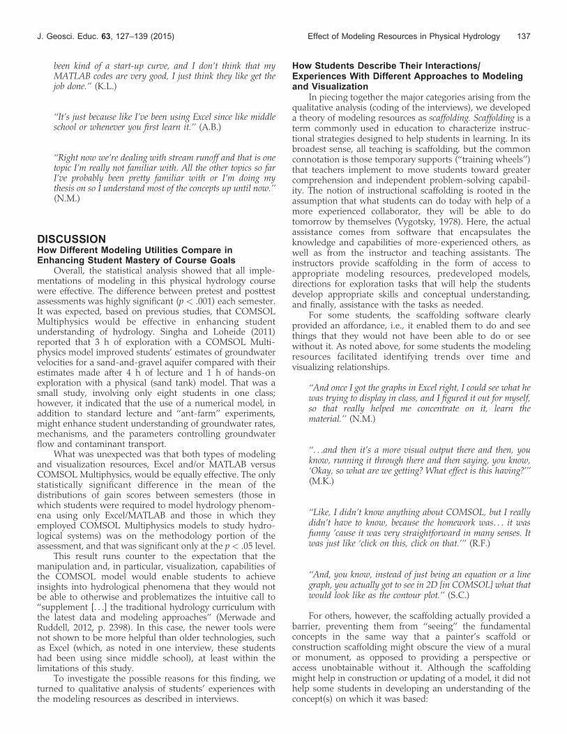
TABLE III: Categories and themes arising from qualitativeanalysis of interviews.

Barriers

Instructions/examples (lack of)

Time

Lack of clear expectations

Affordances

Visualization

Identification of trends

Synthesis

Analysis of data

Relating concepts to equations

Acquiring tools/skills

Preferences

Appreciation/satisfaction

Difficulties/challenges

Familiarity


been kind of a start-up curve, and I don’t think that myMATLAB codes are very good, I just think they like get thejob done.’’ (K.L.)

‘‘It’s just because like I’ve been using Excel since like middleschool or whenever you first learn it.’’ (A.B.)

‘‘Right now we’re dealing with stream runoff and that is onetopic I’m really not familiar with. All the other topics so farI’ve probably been pretty familiar with or I’m doing mythesis on so I understand most of the concepts up until now.’’(N.M.)

DISCUSSIONHow Different Modeling Utilities Compare inEnhancing Student Mastery of Course Goals

Overall, the statistical analysis showed that all imple-mentations of modeling in this physical hydrology coursewere effective. The difference between pretest and posttestassessments was highly significant (p < .001) each semester.It was expected, based on previous studies, that COMSOLMultiphysics would be effective in enhancing studentunderstanding of hydrology. Singha and Loheide (2011)reported that 3 h of exploration with a COMSOL Multi-physics model improved students’ estimates of groundwatervelocities for a sand-and-gravel aquifer compared with theirestimates made after 4 h of lecture and 1 h of hands-onexploration with a physical (sand tank) model. That was asmall study, involving only eight students in one class;however, it indicated that the use of a numerical model, inaddition to standard lecture and ‘‘ant-farm’’ experiments,might enhance student understanding of groundwater rates,mechanisms, and the parameters controlling groundwaterflow and contaminant transport.

What was unexpected was that both types of modelingand visualization resources, Excel and/or MATLAB versusCOMSOL Multiphysics, would be equally effective. The onlystatistically significant difference in the mean of thedistributions of gain scores between semesters (those inwhich students were required to model hydrology phenom-ena using only Excel/MATLAB and those in which theyemployed COMSOL Multiphysics models to study hydro-logical systems) was on the methodology portion of theassessment, and that was significant only at the p < .05 level.

This result runs counter to the expectation that themanipulation and, in particular, visualization, capabilities ofthe COMSOL model would enable students to achieveinsights into hydrological phenomena that they would notbe able to otherwise and problematizes the intuitive call to‘‘supplement [. . .] the traditional hydrology curriculum withthe latest data and modeling approaches’’ (Merwade andRuddell, 2012, p. 2398). In this case, the newer tools werenot shown to be more helpful than older technologies, suchas Excel (which, as noted in one interview, these studentshad been using since middle school), at least within thelimitations of this study.

To investigate the possible reasons for this finding, weturned to qualitative analysis of students’ experiences withthe modeling resources as described in interviews.

How Students Describe Their Interactions/Experiences With Different Approaches to Modelingand Visualization

In piecing together the major categories arising from thequalitative analysis (coding of the interviews), we developeda theory of modeling resources as scaffolding. Scaffolding is aterm commonly used in education to characterize instruc-tional strategies designed to help students in learning. In itsbroadest sense, all teaching is scaffolding, but the commonconnotation is those temporary supports (‘‘training wheels’’)that teachers implement to move students toward greatercomprehension and independent problem-solving capabil-ity. The notion of instructional scaffolding is rooted in theassumption that what students can do today with help of amore experienced collaborator, they will be able to dotomorrow by themselves (Vygotsky, 1978). Here, the actualassistance comes from software that encapsulates theknowledge and capabilities of more-experienced others, aswell as from the instructor and teaching assistants. Theinstructors provide scaffolding in the form of access toappropriate modeling resources, predeveloped models,directions for exploration tasks that will help the studentsdevelop appropriate skills and conceptual understanding,and finally, assistance with the tasks as needed.

For some students, the scaffolding software clearlyprovided an affordance, i.e., it enabled them to do and seethings that they would not have been able to do or seewithout it. As noted above, for some students the modelingresources facilitated identifying trends over time andvisualizing relationships.

‘‘And once I got the graphs in Excel right, I could see what hewas trying to display in class, and I figured it out for myself,so that really helped me concentrate on it, learn thematerial.’’ (N.M.)

‘‘. . .and then it’s a more visual output there and then, youknow, running it through there and then saying, you know,‘Okay, so what are we getting? What effect is this having?’’’(M.K.)

‘‘Like, I didn’t know anything about COMSOL, but I reallydidn’t have to know, because the homework was. . . it wasfunny ’cause it was very straightforward in many senses. Itwas just like ‘click on this, click on that.’’’ (R.F.)

‘‘And, you know, instead of just being an equation or a linegraph, you actually got to see in 2D [in COMSOL] what thatwould look like as the contour plot.’’ (S.C.)

For others, however, the scaffolding actually provided abarrier, preventing them from ‘‘seeing’’ the fundamentalconcepts in the same way that a painter’s scaffold orconstruction scaffolding might obscure the view of a muralor monument, as opposed to providing a perspective oraccess unobtainable without it. Although the scaffoldingmight help in construction or updating of a model, it did nothelp some students in developing an understanding of theconcept(s) on which it was based:


‘‘The reason I would take a physical hydrology course is tosee things come from first principles, to come from physics,and the course material itself is often very encapsulated. . ..We’re provided with like Excel spreadsheets and all thesethings, at least for me, the perspective I want out of the class,these are all barriers to the fundamental, sort of fluiddynamic processes that I’m trying to understand.’’ (D.S.)

The student quoted above clearly did not see thefundamental physics in the outputs of the software. Forhim, the closed-form equations themselves correlated withthe concepts in a way that that the graphs and imagesproduced by the software could not. He would havepreferred ‘‘time and space to engage with the equationsalone, at a level of rigor that I don’t find in class or certainlyin assignments’’ (D.S.).

Another way in which the scaffolding software createdan unintended barrier for the students was in terms of thetime and detailed procedures necessary to produce a result.Students cited this barrier for each of the forms of softwareused:

‘‘But for me, because of my not knowing Excel—not knowinghow to do spreadsheets very well, and not remembering allthe math and physics—it took me probably twice thatamount of time, and I just found that excessive.’’ (P.B.)

‘‘So I think the easiest parts for me on the homework havebeen like conceptual questions, because a lot of the rest has todo with figuring stuff out in MATLAB and plotting it inMATLAB and things like that.’’ (K.L.)

‘‘When I was using the COMSOL, I felt like I was juststruggling with the interface in trying to figure out how Ineed to do what I was suppose to be doing and wondering if Iwas doing the right thing. So, I wasn’t thinking much aboutthe science that was going on. Um, it was more about, ‘did Iclick the right buttons?’’ (A.W.)

The means to remove these two types of barriers mayrun counter to each other. Although the images and displaysmade possible by more-advanced modeling technologiesmight enable novice users to identify trends and synthesizeconcepts, the same technological affordances might hide (orat least not highlight) fundamental features of the physics ofhydrological systems, allowing the user to be unaware of‘‘the limitations and difficulties in developing numericalmodels that faithfully represent the system they aremodeling.’’6

In some cases, even students who benefitted from theaffordances of whichever modeling resources they used andthe access those tools provided to solutions for the novicemodeler, also faced the greatest barriers in using thesoftware:

‘‘Overall, after we can get the Excel to work and then we plotwhatever we’re looking at, that’s definitely beneficial, and itdefinitely helps summarize certain processes or helps you

learn the general trend of things, but getting to that point,often times, is somewhat difficult.’’ (J.P.W.)

‘‘That’s where the science is. . . is like modeling and... So Ithink it is really useful; I think the hurdle (maybe) is (like)the technical, knowing the program, the start-up associatedwith (like) getting to know a program, but once youunderstand it and if you can actually relate it to physicalprocesses, then yeah, I think it’s helpful.’’ (K.L.)

‘‘I got a lot out of [COMSOL modeling], but it was too mucheffort and frustration, and too much time for what I got outof it.’’ (P.B.)

‘‘COMSOL, I kind of wondered at the time why we weredoing it because most of us have never heard of it and willnever use it. And so it was a little bit pointless for most of usin the class, and it took a lot of time. But the visualizationwas pretty neat.’’ (S.C.)

The more powerful, versatile, COMSOL Multiphysicsallowed students to do (and see) more, but was less familiarand more challenging. As noted on the COMSOL Web site:

‘‘Finite element methods for approximating partial differen-tial equations that arise in science and engineering analysisfind widespread application. Numerical analysis tools makethe solutions of coupled physics, mechanics, chemistry, andeven biology accessible to the novice modeler. . . . But withthis modeling power comes great opportunities and greatperils.’’ (emphasis added) (http://www.comsol.com/books/mmwfem).

Thus, despite the affordances provided, all threemodeling resources explored in the course of this study alsocreated barriers to learning, at least for some students. In theend, personal preferences and familiarity had the dominantrole in determining the balance between the two effects.

CONCLUSIONS AND IMPLICATIONSAlthough our quantitative results did not show a clear

advantage for the incorporation of the COMSOL Multi-physics, the qualitative results indicate the value thatstudents placed on the opportunity to learn to use this tool:

‘‘I think that could be really useful, especially withCOMSOL being something that would be very importantto anyone in this room. . . for the hydrologists, that would bevery, very important.’’ (A.J.)

Even students who thought they would never useCOMSOL in the course of their careers saw value in theability to visualize phenomena, and our program remainscommitted to continuing to offer and expand activities withCOMSOL Multiphysics as part of the instruction in physicalhydrology and to make these tools available to the largercommunity. For more information about access to themodules, please contact one of the authors.6 http://www.comsol.com/books/mmwfem.


However, these results also indicate the need both tomake the COMSOL Multiphysics modules more accessibleand to ensure that they are used in such a way that studentsare ‘‘thinking. . . about the science that [is] going on’’ ratherthan thinking ‘‘did I click the right buttons’’ to justify theexpenditure of effort on the part of students and instructorsto include them in the curriculum. Perhaps not surprisingly,these results reiterate that the effectiveness of any tool willdepend on the needs and abilities of the user, and how sheor he uses that tool. A newer, more powerful technology willnot necessarily provide a panacea. Developers need to becognizant of the need to provide self-explanatory andintuitive interfaces, with entry points for more-novice users(training wheels), which still allow the user to inspect andconsider the constraints and boundary conditions that mighthave been implemented on his or her behalf. A major step inthis direction has been a new COMSOL release, calledCOMSOL Server, in which a user (in this case, the instructor)can create a model and ‘‘freeze’’ it for others to use, placinglimitations on the changes that can be made to variables.This feature will be employed in future instantiations of thecourse to make the COMSOL manipulations more trans-parent to the students. Demonstrating that students learnmore (or more efficiently) with the COMSOL modules asthey exist would have been in some ways a more welcomeresult; however, solid evidence that more work needs todone to make the modules accessible to students is also ofvalue.

At the same time, in giving students access to the latestdata and modeling approaches, care needs to be taken thatscaffolding provided does not obscure the physics, withmodeling tasks supplemented by reflection, closing the loopback to the fundamental laws. No amount of modeling andvisualization will substitute for thinking and articulatingwhat the models are telling us. Therefore, open-ended,conceptual questions requiring students to describe themeaning of the simulation results will continue to be part ofCOMSOL-based homework exercises (see online supple-ment4). The ultimate goal is for students to ‘‘put it alltogether and not just schematically, but . . .with some sort ofphysically derived equation,’’ as A.J. did.

Finally, this study took place in only one course at oneinstitution. Not all students consented to participate, and notall participants completed both the pretest and the posttestassessment, limiting the generalizability of the results.Further, participant numbers were not sufficient to bedisaggregated by student status (undergraduate versusgraduate), gender, or, perhaps more important, by thestudent’s intended career path. Thus, another outcome ofthis study is the identification of the need for further researchinto the effectiveness of the COMSOL Multiphysics curric-ulum intervention described here with larger populations.

AcknowledgmentsThe authors gratefully acknowledge the support from

the U.S. National Science Foundation CAREER grant EAR-0955750, University of Texas, College of Education, graduateresearch funding, and the Geology Foundation at theUniversity of Texas, Austin. We thank Kevin Befus, AlecNorman, Lichun Wang, and Peter Zamora for theirassistance in coding the data.

REFERENCESDingman, S.L. 2008. Physical hydrology. Long Grove, IL: Waveland

Press.Groves, J.R., and Moody, D.W. 1992. A survey of hydrology course

content in North American universities. Water ResourcesBulletin, 28(3):615–621.

Manduca, C.A., Baer, E., Hancock, G., Macdonald, R.H., Patterson,S., Savina, M., and Wenner, J. 2008. Making undergraduategeoscience quantitative. EOS, 89(16):149–150.

Mann, M.P. 1993. Grounded theory and classroom research. Journalon Excellence in College Teaching, 4:131–143.

Marshall, J.A., Castillo, A.J., and Cardenas, M.B. 2013. Assessingstudent understanding of physical hydrology. Hydrology andEarth System Sciences, 17:829–836. doi: 10.5194/hess-17-829-2013.

Merwade, V., and Ruddell, B.L. 2012. Moving university hydrologyeducation forward with community-based geoinformatics,data and modeling resources. Hydrology and Earth SystemSciences, 16:2393–2404. doi:10.5194/hess-16-2393-2012.

Nash, J.E., Eagleson, P.S., Philip, J.R., van der Molen, W.H., andKlemes, V. 1990. The education of hydrologists (Report of anIAHS/UNESCO panel on hydrological education). HydrologicalS c i e n c e s J o u r n a l , 3 5 ( 6 ) : 5 9 7 – 6 0 7 . d o i : 1 0 . 1 0 8 0 /02626669009492466.

Singha, K., and Loheide, S.P II. 2011. Linking physical andnumerical modelling in hydrogeology using sand tankexperiments and COMSOL Multiphysics. International Journalof Science Education, 33(4):547–571.

Vygotsky, L.S. 1978. Mind in society. Cambridge, MA: HarvardUniversity Press.

Wagener, T., Kelleher, C., Weiler, M., McGlynn, B., Gooseff, M.,Marshall, L., Meixner, T., McGuire, K., Gregg, S., Sharma, P.,and Zappe, S. 2012. It takes a community to raise ahydrologist: The Modular Curriculum for Hydrologic Advance-ment (MOCHA). Hydrology and Earth System Sciences, 16:3405–3418, doi:10.5194/hess-16-3405.

Wagener, T., Sivapalan, M., Troch, P.A., McGlynn, B.L., Harman,C.J., Gupta, H.V., Kumar, P., Rao, P.S.C., Basu, N.B., andWilson, J.S. 2010. The future of hydrology: An evolving sciencefor a changing world. Water Resources Research, 46(5):W05301,doi:10.1029/2009WR008906.

Wagener, T., Weiler, M., McGlynn, B., Gooseff, M., Meixner, T.,Marshall, L., McGuire, K., and McHale, M. 2007. Taking thepulse of hydrology education. Hydrological Processes,21(13):1789–1792.

Zimmerman, W.B.J. 2006. Multiphysics modeling with finiteelement methods. Singapore: World Scientific.


Documents

The Effect of Modeling and Visualization Resources on ... · The Effect of Modeling and Visualization Resources on Student Understanding of Physical Hydrology Jill A. Marshall,1,a