Embed Size (px)
Citation preview
University of New MexicoUNM Digital Repository
Civil Engineering ETDs Engineering ETDs
7-3-2012
The effect of mica on the aging of asphalt binderHelen Sobien
Follow this and additional works at: https://digitalrepository.unm.edu/ce_etds
This Thesis is brought to you for free and open access by the Engineering ETDs at UNM Digital Repository. It has been accepted for inclusion in CivilEngineering ETDs by an authorized administrator of UNM Digital Repository. For more information, please contact [email protected].
Recommended CitationSobien, Helen. "The effect of mica on the aging of asphalt binder." (2012). https://digitalrepository.unm.edu/ce_etds/64

i
Helen Marie Sobien
Candidate
Civil Engineering
Department
This thesis is approved, and it is acceptable in quality
and form for publication:
Approved by the Thesis Committee:
Dr. Rafiqul Tarefder , Chairperson
Dr. Mahmoud Reda Taha
Dr. John C. Stormont
EFFECT OF MICA ON ASPHALT
BINDER AGING BEHAVIOR
BY
HELEN MARIE SOBIEN
Bachelor of Science, Civil Engineering,
University of New Mexico
Dec 2009
THESIS
Submitted in Partial Fulfillment of the
Requirements for the Degree of
Master of Science
Civil Engineering
The University of New Mexico
Albuquerque, New Mexico
May, 2012

iii
DEDICATION
To my family.

iv
Acknowledgements
From the bottom of my heart, I thank Dr. Rafiqul Tarefder, my professor and adviser, for
his assistance, without which I would not have been able to complete the first semester in
the Civil Engineering program, let alone continue to graduate school. Also, for his
continuing mentorship and financial support which saw me through the Master’s
program. I will never forget the encouragement he has given to me. Thanks to my
Thesis Committee members for their efforts on my behalf. Thanks to the New Mexico
Space Grant Consortium for funding one year of my graduate studies and to the National
Science Foundation for funding my work.
Thanks to Dr. Mahmoud R. Taha for his continuing encouragement for the last five years.
For their efforts toward completing this thesis, thanks to: Lorenzo Gutierrez, who served
as a guide to a mica source in the wilderness, Pancho Sobien and Katherine Rodriguez,
for their efforts to find and grind mica, Hasan Mohammad Faisal for helping me with
nanoindentation tests, Jim Connolly for running the XRD tests and guidance in
mineralogy and Dr. Ying-Bing Jiang for help with the SEM;
Also, thanks to Robert Sandoval, NMDOT, for his many efforts at guiding and training
me over the last 3 years, and for the loan of equipment. Thanks to Dr. Arif Zaman for his
instruction when I first entered the asphalt program. Finally, thanks to Lafarge
Albuquerque and Holly Asphalt for providing material, especially to Ray Cruz and
Angelica Alvarado.
v
EFFECT OF MICA ON ASPHALT
BINDER AGING BEHAVIOR
by
Helen Marie Sobien
B.S., Civil Engineering, University of New Mexico, 2009
M.S., Civil Engineering, University of New Mexico, 2012
ABSTRACT
Asphalt Concrete (AC) consists of approximately 95% aggregate, by weight. Of this
95%, about 6% is smaller than 0.075 mm in size (passing the #200 sieve and called
fines). The fines often contain mica. Mica is a formation of silicate minerals having
perfect basal cleavage. It can be peeled apart in very thin sheets and is usually found in
deposits of granite, quartz and other rock that is commonly used for aggregate. Mica has
been shown to reduce the strength of asphalt concrete. This study evaluates the effects of
mica on asphalt materials subjected to aging.
A total of five different concentrations of mica in fines are examined using X-ray
diffraction (XRD) technology. These mica-fines are combined with two asphalt binders
to make mastics. Mastics are aged at four different levels and examined with the
Scanning Electron Microscope (SEM). Bending Beam Rheometer (BBR) and
nanoindentation tests are conducted on mastics mixed with one of the binders and various
concentrations of mica-fines aged at different levels.
In this study, SEM images of mastic are taken. During the mixing of the mastics, it is
found that as the concentration of mica in the fines increases, so does the absorption of
the binder. This is probably because mica has a flat surface that increases the surface
vi
area of the total aggregate. As the weight percentages of aggregate to binder is held
exactly constant in the experiments conducted in this study, the mastics with lower
concentrations of mica are found to be very rich while the higher concentrations are dry.
SEM images show that cracks in broken mastic seem to follow uncoated mica flakes. The
number of uncoated flakes increases only slightly with aging, but quite dramatically with
mica concentration.
XRD is used to identify and roughly quantify the amount of mica in aggregate. Spectra
from samples of single-source fines, containing varying quantities of mica, clearly
indicate the change in mica content. However, when a known quantity of mica is added
to fines of different aggregate sources, the spectrum generated shows little in common
with the previous samples, which makes it difficult to estimate the mica content. XRD
analysis is most repeatable when crystals are randomly oriented in the sample. Because
mica flakes tends to lie flat, they tend to be somewhat ordered in their orientation,
particularly when the grains of material are much larger than 1 micron. Hence, while the
XRD is a powerful tool for helping determine the presence of mica, its limitations are
evident from this study.
Nanoindentation is used to determine the hardness and stiffness of mica-mastic at the
micro scale. It is shown that mastic with no mica becomes much harder after long term
aging, indicating embrittlement. Mastic with low concentrations of mica is shown to be
only a little harder. Mastic with 10% mica becomes softer after long term aging.
The more traditional test of BBR is used to study the mica-mastic at a macro scale and
varying temperature. The results of this experiment confirmed the unexpected results of

vii
the nanoindenter. Mastic with less than 5% mica in the fines behaves similarly to binder.
However, at a mica content of 10%, the stiffness decreases after long term aging. This
might suggest that mica reduces aging effects.
viii
TABLE OF CONTENTS
ABSTRACT ........................................................................................................................v
LIST OF FIGURES ......................................................................................................... xi
LIST OF TABLES ......................................................................................................... xiv
CHAPTER 1 INTRODUCTION ......................................................................................1
1.1 Introduction .........................................................................................................1
1.2 Objectives ............................................................................................................3
1.3 Organization of Thesis ........................................................................................4
CHAPTER 2 LITERATURE REVIEW ..........................................................................5
2.1 Mica.....................................................................................................................5
2.2 Identifying Mica ..................................................................................................6
2.3 Mica’s Influence on Mechanical Properties ........................................................8
2.4 Particle Shape and Surface Area .........................................................................8
2.5 Effects of Mineral Filler on Mastic .....................................................................9
2.6 NCHRP Reports ................................................................................................11
2.7 Aging .................................................................................................................13
2.8 X-ray Diffraction (XRD)...................................................................................14
2.9 Scanning Electron Microscope (SEM)..............................................................16
2.10 Energy Dispersive X-ray (EDX) .......................................................................17
2.11 Nanoindentation ................................................................................................18
2.12 Bending Beam Rheometer (BBR) .....................................................................21
ix
CHAPTER 3 METHODOLOGY ...................................................................................35
3.1 Mica...................................................................................................................35
3.2 XRD ..................................................................................................................36
3.3 Mixing and molding mastic ..............................................................................37
3.4 SEM Sample Preparation ..................................................................................39
3.5 Nanoindentation ................................................................................................40
3.6 BBR ...................................................................................................................42
CHAPTER 4 SEM ANALYSIS OF MASTIC MICA ..................................................65
4.1 Introduction .......................................................................................................65
4.2 Viewing mastics ................................................................................................65
4.3 Conclusion ........................................................................................................70
CHAPTER 5 XRD ANALYSIS OF MICA IN FINES .................................................82
5.1 Introduction .......................................................................................................88
5.2 Analysis .............................................................................................................88
5.2.1 Theory of XRD .....................................................................................88
5.2.2 100% mica sample ................................................................................89
5.2.3 100% fines sample ................................................................................89
5.2.4 10% mica in fines ..................................................................................90
5.2.5 2.5, 5 and 7.5% mica in fines ................................................................90
123 5.2.6 Two fines sources compared .................................................................91
5.3 Conclusion .........................................................................................................92
x
CHAPTER 6 ANALYSIS OF NANOINDENTATION ON MASTIC-MICA ...........98
6.1 Introduction .......................................................................................................98
6.2 Unmodified Binder Samples .............................................................................98
6.3 SB4% modified Binder Samples .....................................................................100
6.4 Conclusions .....................................................................................................104
CHAPTER 7 ANALYSIS BENDING BEAM RHEOMETER TESTS ON
MASTIC MICA ..................................................................................115
7.1 Introduction .....................................................................................................115
7.2 Test Results .....................................................................................................115
7.3 Conclusion ......................................................................................................117
CHAPTER 8 CONCLUSIONS ....................................................................................124
8.1 Introduction .....................................................................................................124
8.2 XRD ................................................................................................................124
8.3 SEM ................................................................................................................125
8.4 Nanoindenter ...................................................................................................126
8.5 BBR .................................................................................................................127
8.6 Conclusions .....................................................................................................127
8.7 Recommendations ...........................................................................................128
REFERENCES ...............................................................................................................129
APPENDIX I ..................................................................................................................135
xi
LIST OF FIGURES
Figure 2.1 Specimen of muscovite ..............................................................................22
Figure 2.2 Paper model of muscovite ..........................................................................23
Figure 2.3 Paper model of quartz ................................................................................24
Figure 2.4 Illustration of X-ray beam waves ...............................................................25
Figure 2.5 Illustration X-rays striking crystalline material .........................................26
Figure 2.6 XRD spectra of muscovite and feldspar ....................................................27
Figure 2.7 Schematic of SEM .....................................................................................28
Figure 2.8 Electron beams entering atom ....................................................................29
Figure 2.9 Nanoindenter tip and its impression ..........................................................30
Figure 2.10 Load displacement curves for nanoindenter ..............................................31
Figure2.11 Cut-away view of indentation ....................................................................32
Figure2.12 Schematic of BBR......................................................................................33
Figure 2.13 Graph of m-value slope ..............................................................................34
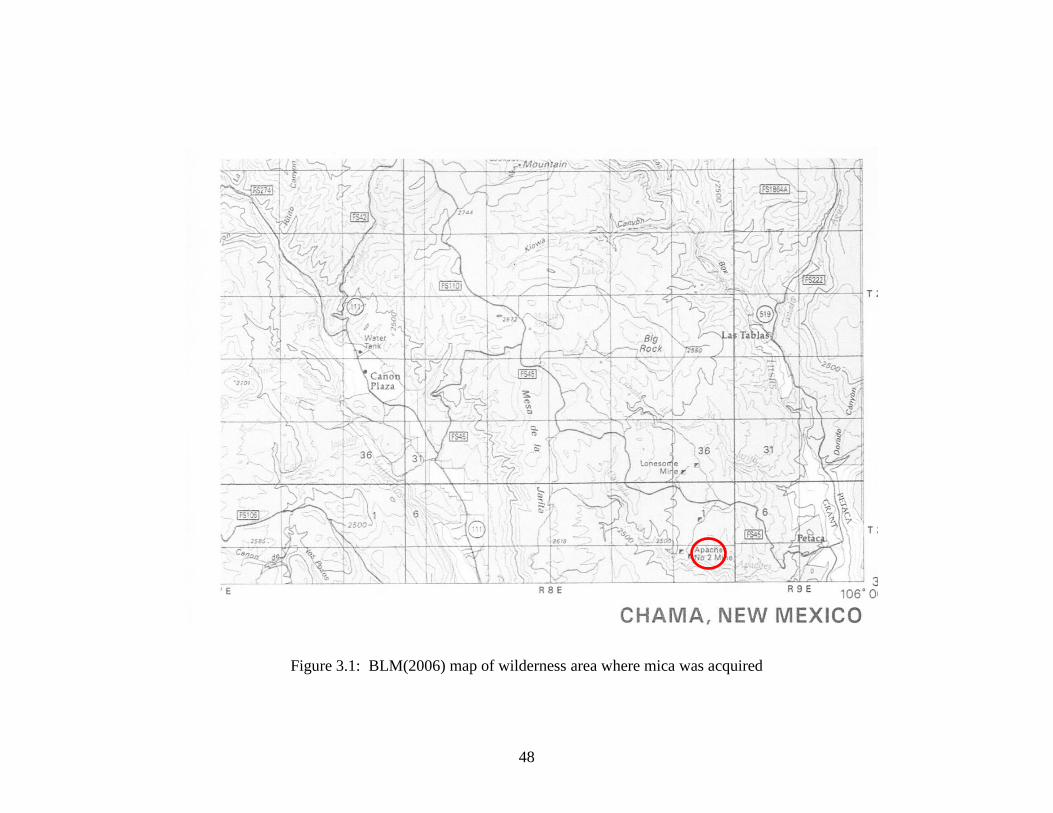
Figure 3.1 Map of mica source ....................................................................................48
Figure 3.2 Mica ...........................................................................................................49
Figure 3.3 XRD samples .............................................................................................50
Figure 3.4 Mastics with 21% binder ...........................................................................51
Figure 3.5 RTFO jars...................................................................................................52
Figure 3.6 Mastics with 19.5% binder .......................................................................53
Figure 3.7 Samples for SEM .......................................................................................54
Figure 3.8 Compaction and breakage of SEM samples ..............................................55
Figure 3.9 SEM sample preparation ............................................................................56
xii
Figure 3.10 SEM equipment .........................................................................................57
Figure 3.11 Nanoindenter sample manufacture ............................................................58
Figure 3.12 Nanoindenter samples ................................................................................59
Figure 3.13 Sample mounted in nanoindenter...............................................................60
Figure 3.14 Pattern of indentations ...............................................................................61
Figure 3.15 BBR equipment ..........................................................................................62
Figure 3.16 BBR sample molds ....................................................................................63
Figure 3.17 Compaction of BBR samples .....................................................................64
Figure 4.1 Original AC sample ...................................................................................72
Figure 4.2 SEM and EDX of mica powder .................................................................73
Figure 4.3 SEM and EDX of 10% mica-fines .............................................................74
Figure 4.4 SEM and EDX of 100-fines .......................................................................75
Figure 4.5 EDX of two grains in sample .....................................................................76
Figure 4.6 SEM of 2.5% mica .....................................................................................77
Figure 4.7 SEM of 5% mica ........................................................................................77
Figure 4.8 SEM of mica in 5% sample .......................................................................78
Figure 4.9 SEM of piece that crumbled off .................................................................79
Figure 4.10 SEM of flat area of same sample ...............................................................80
Figure 4.11 SEM of 2.5% mica, high magnification .....................................................81
Figure 4.12 SEM and EDX of 2.5% .............................................................................82
Figure 4.13 SEM and EDX of 0% ................................................................................83
Figure 5.1 XRD pattern of mica ..................................................................................94
Figure 5.2 XRD patterns of 5 samples compared .......................................................95
xiii
Figure 5.3 Close analysis of XRD of five concentrations ..........................................96
Figure 5.4 Comparison of XRD of two fines sources .................................................97
Figure 6.1 Nanoindentation test curves for unmodified samples ..............................105
Figure 6.2 Graphs hardness, stiffness vs. mica content Unmodified ........................107
Figure 6.3 SEM images of nanoindentation samples ................................................108
Figure 6.4 Graphs hardness, stiffness from nanoindentation of SB4%.....................110
Figure 6.5 Graph comparing nanoindentation results RTFO 10% samples ..............112
Figure 6.6 Graphs comparing stiffness and hardness ................................................113
Figure 6.7 Creep Compliance curves ........................................................................114
Figure 7.1 Graph of sample densities ........................................................................119
Figure 7.2 Graph of sample stiffness at t-60 .............................................................121
Figure 7.3 Graph of sample stiffness at t-120 ...........................................................122
Figure 7.4 Graph of sample stiffness at t-240 ...........................................................123
xiv
LIST OF TABLES
Table 3.1 XRD test matrix .........................................................................................44
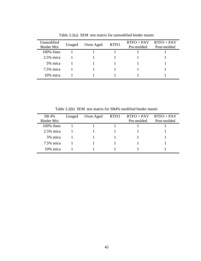
Table 3.2 SEM test matrices ......................................................................................45
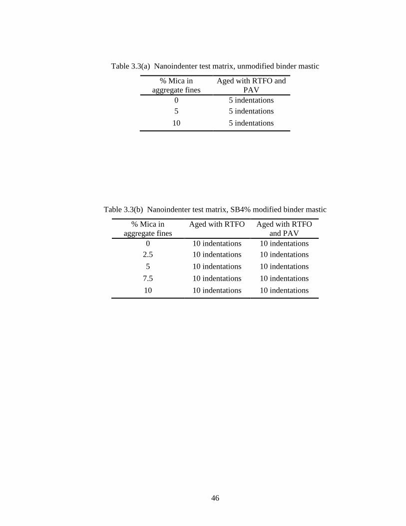
Table 3.3 Nanoindenter test matrices .........................................................................46
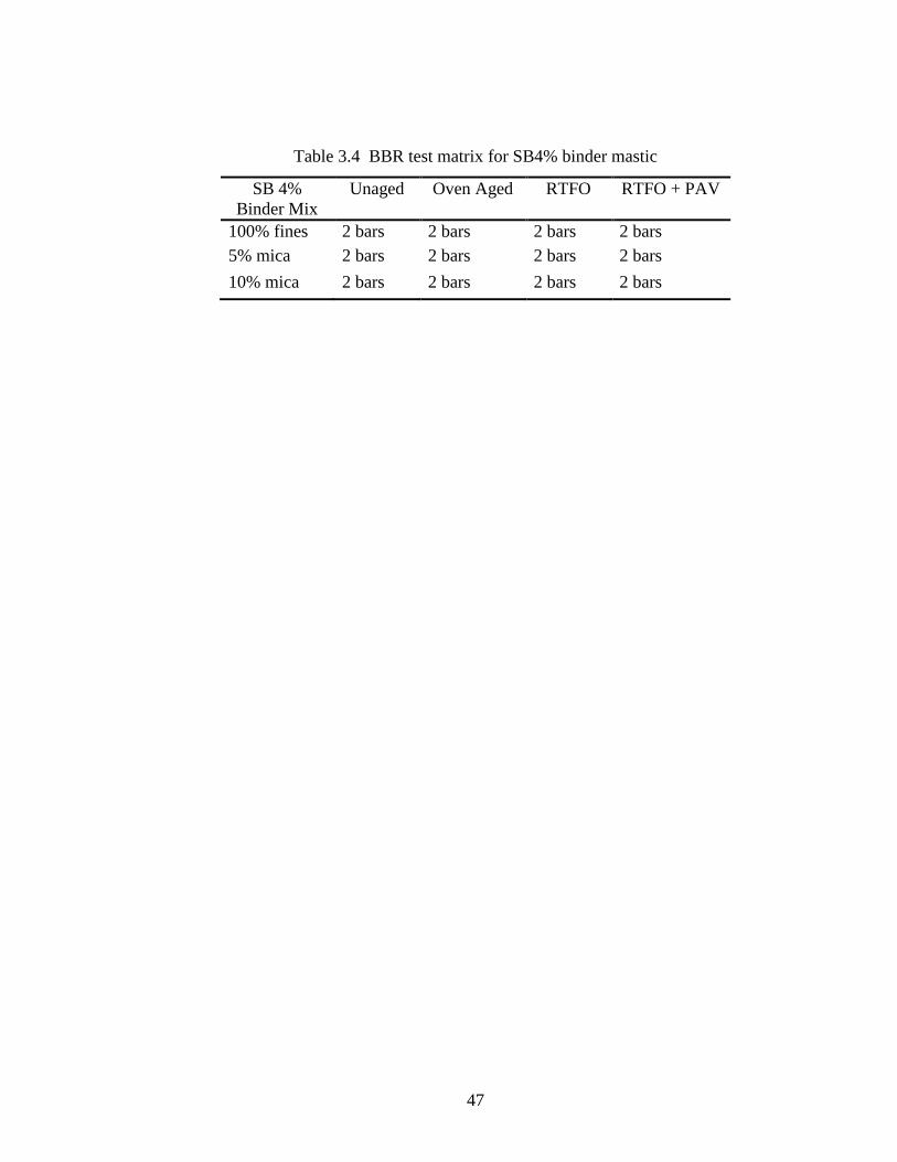
Table 3.4 BBR test matrix..........................................................................................47
Table 4.1 Summary flake counts Unmodified ...........................................................84
Table 4.2 General observations Unmodified .............................................................85
Table 4.3 Summary flake counts SB4% ....................................................................86
Table 4.4 General observations SB4% ......................................................................87
Table 6.1 Hardness, stiffness data unmodified mastics nanoindentation ................106
Table 6.2 Hardness, stiffness data modified mastics nanoindentation ....................109
Table 6.3 Comparison 10% mica RTFO samples ....................................................111
Table 7.1 Sample dimensions and densities.............................................................118
Table 7.2 BBR stiffness data....................................................................................120
1
CHAPTER 1
INTRODUCTION
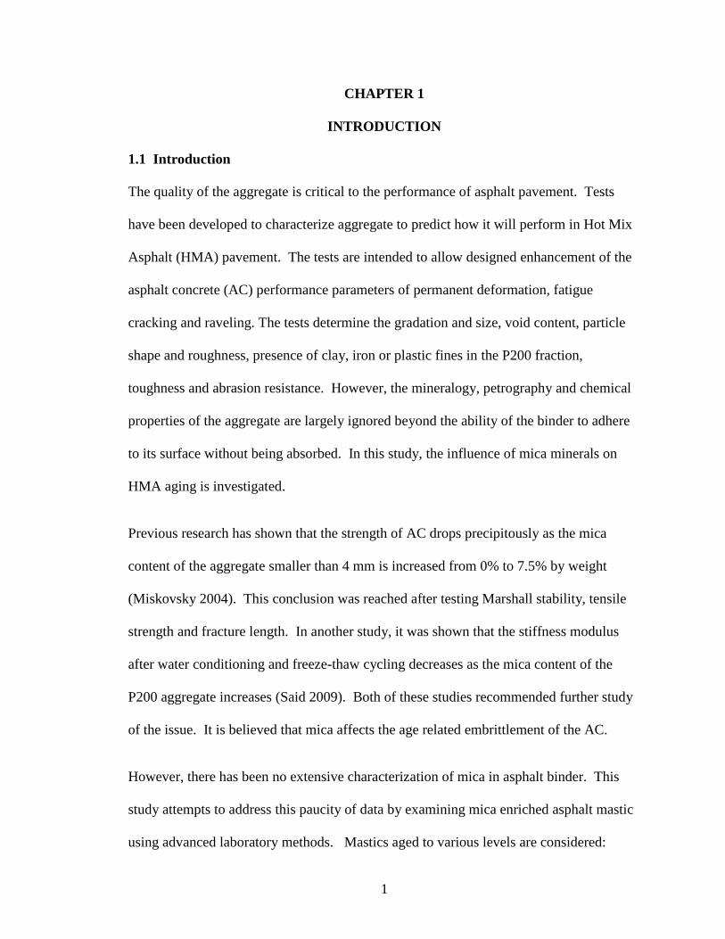
1.1 Introduction
The quality of the aggregate is critical to the performance of asphalt pavement. Tests
have been developed to characterize aggregate to predict how it will perform in Hot Mix
Asphalt (HMA) pavement. The tests are intended to allow designed enhancement of the
asphalt concrete (AC) performance parameters of permanent deformation, fatigue
cracking and raveling. The tests determine the gradation and size, void content, particle
shape and roughness, presence of clay, iron or plastic fines in the P200 fraction,
toughness and abrasion resistance. However, the mineralogy, petrography and chemical
properties of the aggregate are largely ignored beyond the ability of the binder to adhere
to its surface without being absorbed. In this study, the influence of mica minerals on
HMA aging is investigated.
Previous research has shown that the strength of AC drops precipitously as the mica
content of the aggregate smaller than 4 mm is increased from 0% to 7.5% by weight
(Miskovsky 2004). This conclusion was reached after testing Marshall stability, tensile
strength and fracture length. In another study, it was shown that the stiffness modulus
after water conditioning and freeze-thaw cycling decreases as the mica content of the
P200 aggregate increases (Said 2009). Both of these studies recommended further study
of the issue. It is believed that mica affects the age related embrittlement of the AC.
However, there has been no extensive characterization of mica in asphalt binder. This
study attempts to address this paucity of data by examining mica enriched asphalt mastic
using advanced laboratory methods. Mastics aged to various levels are considered:
2
unaged, oven aged with a convection oven, short-term aged with the Rolling Thin Film
Oven (RTFO) and long-term aged with the Pressure Aging Vessel (PAV).While previous
work has attempted to identify the presence of mica in aggregates by using existing
traditional aggregate tests, this study attempts to identify and quantify mica in aggregate
fines using the more advanced and reliable techniques of scanning electron microscopy
(SEM) and X-ray diffraction (XRD). SEM is used again to examine fractures in
compacted mastic to determine where it breaks. Finally, the nanoindenter and bending
beam rheometer (BBR) are used to compare the hardness and stiffness between all the
samples. Some of the experiments are done with both unmodified and styrene-butadiene
(SB) polymer modified binders. Some are done using only binder modified with SB
polymer at 4% concentration. Previous studies were done on mica concentrations from
0% to 7.5% in different portions of the aggregate. This study expands the mica
concentration from 0%, as the control group, to 10%, focusing only on the P200 portion.
There are places in the world, including along the Ganges River in Asia, where mica
concentrations in the P200 portions of the soil exceed 10% (Chakrapani et. al 1995).
The mica mineral group represents 37 different minerals, the most common being
Muscovite or potassium mica with the chemical formula KAl2(AlSi3O10)(OH)2 (Dolly
2008). Mica is similar to a book in that it is strong in compression in three dimensions
and strong in tension in two dimensions, but in the third dimension it is weaker in tension
and can be split or peeled apart (Klein and Hurlbut 1993). Mica is found on all seven
continents, often in concentrations high enough to mine for industrial applications.
AASHTO T 240 qualifies the Rolling Thin Film Oven (RTFO) test as adequate
simulation of short term aging; that is, it indicates the approximate change in properties

3
of asphalt incurred during conventional hot-mixing for pavement construction.
AASHTO R 28 qualifies the Pressure Aging Vessel (PAV) as adequate simulation of
long term aging; that is, it can be used to estimate changes in asphalt in service on a
roadway for five to ten years. Much of the work in the literature is based on using these
two accelerated aging methods, and they are employed for aging simulation in this study
as well.
1.2 Objectives
The main objectives of this study are to:
1. Identify and quantify the presence of mica in aggregate fines using analytical
devices including XRD and SEM.
2. Characterize the mechanical properties of mica enriched asphalt mastic at various
levels of aging using nanoindentation and BBR.
4
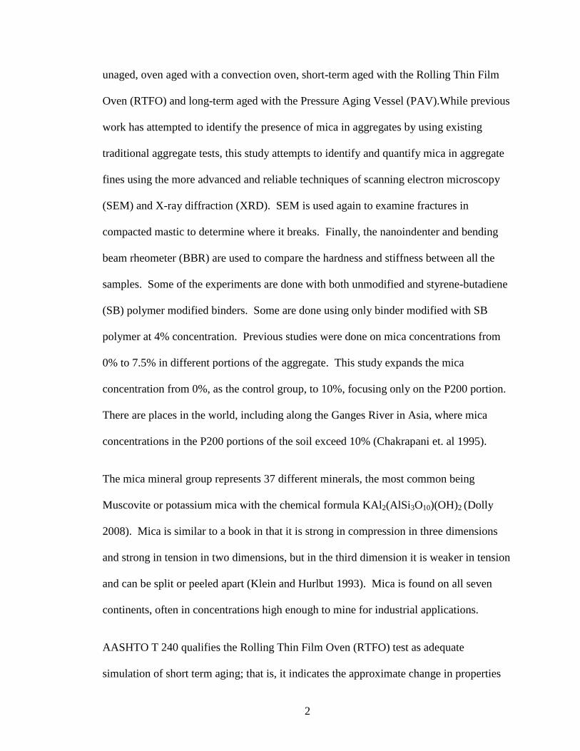
1.3 Organization of Thesis
Chapter 1 defines the need for and objectives of this study. Chapter 2 provides a literature
review of work that has been performed investigating mica and other minerals in mastic
and asphalt concrete, the nature and petrology of mica, US federal guidelines for testing
aggregate and the philosophies of different analytical equipment. Chapter 3 provides a
discussion of the methodology and sample preparation used in this study. Chapter 4
describes the images of fines and mastics seen on the SEM and discusses the implications
of these findings. Chapter 5 provides the results of experiments done with the XRD
identifying and quantifying mica in fines. Chapter 6 presents the results of the
experiments done with the nanoindenter and discusses the mechanical properties of
mastic at high mica concentrations. Chapter 7 presents the results of BBR testing and
discusses the implications of this more traditional test. Lastly, Chapter 8 presents the
final discussion, conclusion and recommendations for future work. Details of SEM
readings are summarized in Appendix I.
5
CHAPTER 2
LITERATURE REVIEW
2.1 Mica
Mica is a family of complex aluminum silicate minerals (sheet silicates) which exhibit
almost perfect basal cleavage (Willmer 1993). That is, it can be split or peeled into thin
sheets or films that are tough, flexible, elastic and, often, transparent. The mica group
represents thirty-seven phyllosilicate minerals that have a layered or platy texture (Dolley
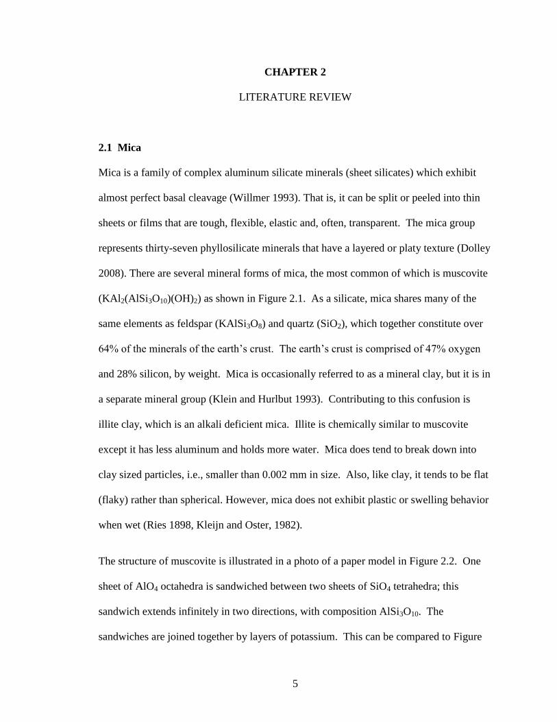
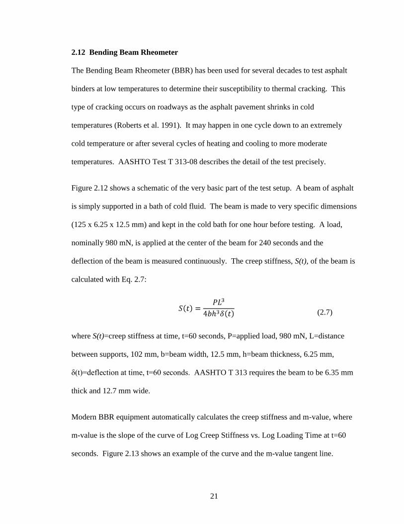
2008). There are several mineral forms of mica, the most common of which is muscovite
(KAl2(AlSi3O10)(OH)2) as shown in Figure 2.1. As a silicate, mica shares many of the
same elements as feldspar (KAlSi3O8) and quartz (SiO2), which together constitute over
64% of the minerals of the earth’s crust. The earth’s crust is comprised of 47% oxygen
and 28% silicon, by weight. Mica is occasionally referred to as a mineral clay, but it is in
a separate mineral group (Klein and Hurlbut 1993). Contributing to this confusion is
illite clay, which is an alkali deficient mica. Illite is chemically similar to muscovite
except it has less aluminum and holds more water. Mica does tend to break down into
clay sized particles, i.e., smaller than 0.002 mm in size. Also, like clay, it tends to be flat
(flaky) rather than spherical. However, mica does not exhibit plastic or swelling behavior
when wet (Ries 1898, Kleijn and Oster, 1982).
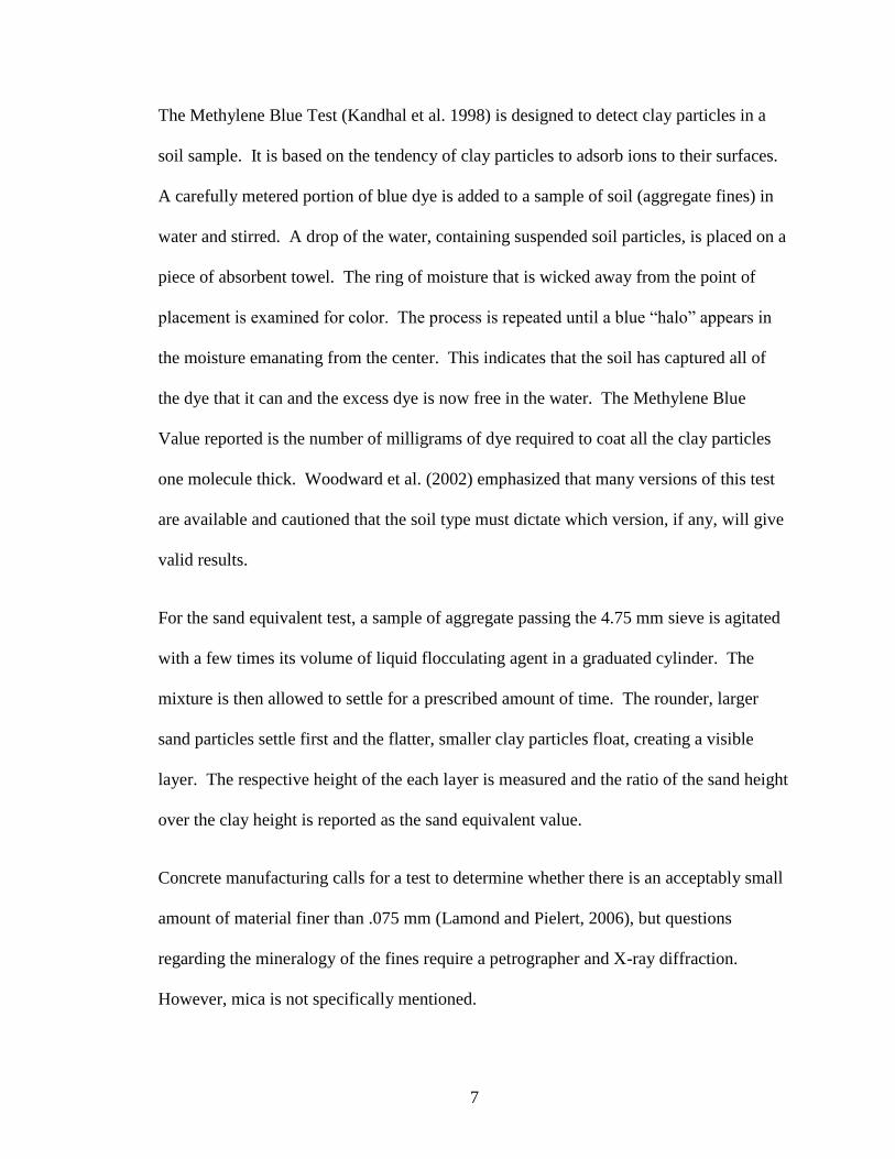
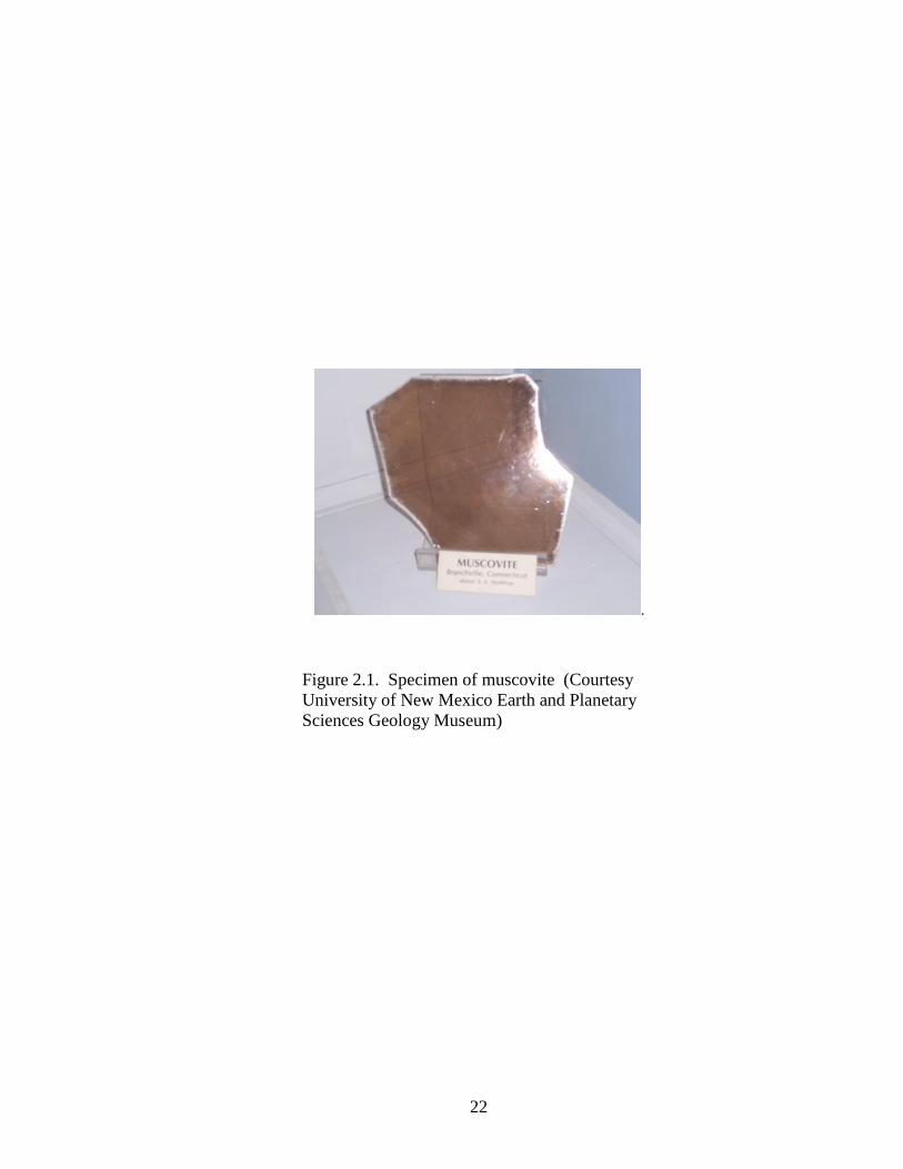
The structure of muscovite is illustrated in a photo of a paper model in Figure 2.2. One
sheet of AlO4 octahedra is sandwiched between two sheets of SiO4 tetrahedra; this
sandwich extends infinitely in two directions, with composition AlSi3O10. The
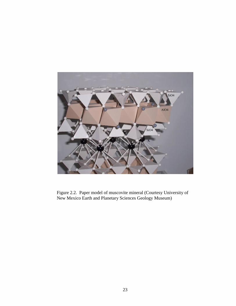
sandwiches are joined together by layers of potassium. This can be compared to Figure
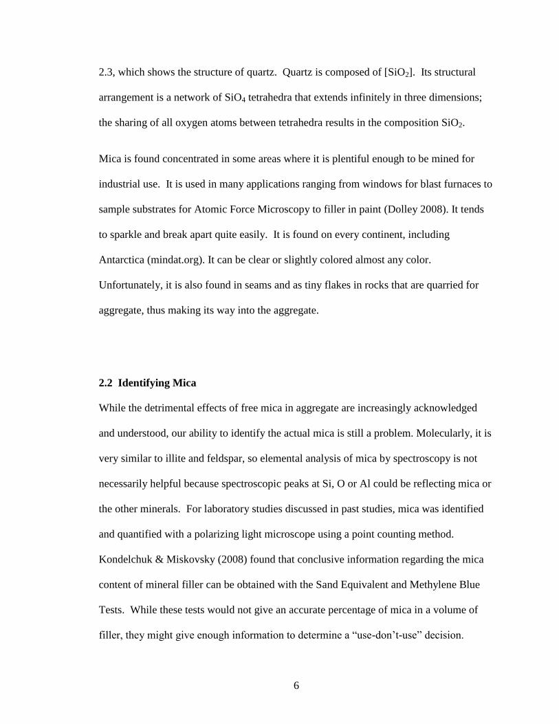
6
2.3, which shows the structure of quartz. Quartz is composed of [SiO2]. Its structural
arrangement is a network of SiO4 tetrahedra that extends infinitely in three dimensions;
the sharing of all oxygen atoms between tetrahedra results in the composition SiO2.
Mica is found concentrated in some areas where it is plentiful enough to be mined for
industrial use. It is used in many applications ranging from windows for blast furnaces to
sample substrates for Atomic Force Microscopy to filler in paint (Dolley 2008). It tends
to sparkle and break apart quite easily. It is found on every continent, including
Antarctica (mindat.org). It can be clear or slightly colored almost any color.
Unfortunately, it is also found in seams and as tiny flakes in rocks that are quarried for
aggregate, thus making its way into the aggregate.
2.2 Identifying Mica
While the detrimental effects of free mica in aggregate are increasingly acknowledged
and understood, our ability to identify the actual mica is still a problem. Molecularly, it is
very similar to illite and feldspar, so elemental analysis of mica by spectroscopy is not
necessarily helpful because spectroscopic peaks at Si, O or Al could be reflecting mica or
the other minerals. For laboratory studies discussed in past studies, mica was identified
and quantified with a polarizing light microscope using a point counting method.
Kondelchuk & Miskovsky (2008) found that conclusive information regarding the mica
content of mineral filler can be obtained with the Sand Equivalent and Methylene Blue
Tests. While these tests would not give an accurate percentage of mica in a volume of
filler, they might give enough information to determine a “use-don’t-use” decision.
7
The Methylene Blue Test (Kandhal et al. 1998) is designed to detect clay particles in a
soil sample. It is based on the tendency of clay particles to adsorb ions to their surfaces.
A carefully metered portion of blue dye is added to a sample of soil (aggregate fines) in
water and stirred. A drop of the water, containing suspended soil particles, is placed on a
piece of absorbent towel. The ring of moisture that is wicked away from the point of
placement is examined for color. The process is repeated until a blue “halo” appears in
the moisture emanating from the center. This indicates that the soil has captured all of
the dye that it can and the excess dye is now free in the water. The Methylene Blue
Value reported is the number of milligrams of dye required to coat all the clay particles
one molecule thick. Woodward et al. (2002) emphasized that many versions of this test
are available and cautioned that the soil type must dictate which version, if any, will give
valid results.
For the sand equivalent test, a sample of aggregate passing the 4.75 mm sieve is agitated
with a few times its volume of liquid flocculating agent in a graduated cylinder. The
mixture is then allowed to settle for a prescribed amount of time. The rounder, larger
sand particles settle first and the flatter, smaller clay particles float, creating a visible
layer. The respective height of the each layer is measured and the ratio of the sand height
over the clay height is reported as the sand equivalent value.
Concrete manufacturing calls for a test to determine whether there is an acceptably small
amount of material finer than .075 mm (Lamond and Pielert, 2006), but questions
regarding the mineralogy of the fines require a petrographer and X-ray diffraction.
However, mica is not specifically mentioned.
8
2.3 Mica’s Influence on Mechanical Properties
When mica-bearing rock is crushed, the highest concentration of free mica is found in the
smallest particle sizes of the aggregate fines (Miskovsky 2004). Also, as the weight
percentage of mica in a bituminous mixture increases, its pavement performance
properties suffer. Using samples prepared according to the Marshall Method, this study
found that, as the weight percentage of free mica increases from 0 to 7.5%, the bulk
density of the mixture drops by 13%, the void ratio increases 22 times, the Marshall
stability drops nearly 90%, the tensile strength drops nearly 75% and fractures increase or
extend more than double. This work was done using a polarizing light microscope, called
a petrographic microscope to count points of mica. The petrographic microscope, which
has two polarizing plates, one above the sample and one below, can be used to identify a
mineral by its index of refraction or by the behavior of light as it passes through a crystal.
The actual aggregate sizes or fines percentages used in the Miskovsky (2004) study were
not detailed in the literature.
2.4 Particle Shape and Surface Area
Said et al. (2009) studied the actual mica grain. It was shown that 100 grams of mica
fines occupies more than double the volume of 100 grams of other mineral fines. This
indicates that the shape of the mica particle gives it a much higher specific surface area.
According to the USGS Minerals Survey (2008), mica layers can be peeled thinner than
25 micrometers. The Specific Surface Area (SSA) of a material increases dramatically as
particles change shape from spherical to flat. For example, a single sphere of volume 1
mm3 would have a surface area of 4.83 mm
2 whereas a disk of the same volume, 25
9
micrometers thick, would have a surface area of 80 mm2. As such, it would require more
binder to coat the fines containing mica enough to insulate against moisture.
Holding the total weight of the mineral fines constant as increasing percentages were
replaced with mica, it was shown that the effort required to compact the test samples
increased dramatically to achieve cylinders with equal air void contents. Also, as the
mica content increased, the stiffness modulus decreased after water conditioning and
freeze-thaw cycling when tested by indirect tensile stress. Similar, but less extreme,
results were found when working by volume instead of weight. A comparison of mineral
fines from five different quarries in Sweden (Said et al. 2009) confirmed that, as mica
content increases, Specific Surface Area increases, the Rigden Void number increases
and stiffness modulus after aging decreases. The Rigden Void number reflects the
volume of voids in a compacted, dry sample of mineral fines.
Said et al. (2009) concluded that increasing the amount of asphalt binder in the mix
would prevent the problem with moisture damage, but did not address rutting or any
other performance properties of pavement.
2.5 Effects of Mineral Filler on Mastic
Anderson et al. (1992) discussed some of the findings of the early SHRP microscopic
studies of mastic. The majority of the surface area generated by the aggregate is in the
fines portion. Also, the fines are embedded in the binder. As such, most of the interaction
between the binder and the aggregate is in the fines.
10
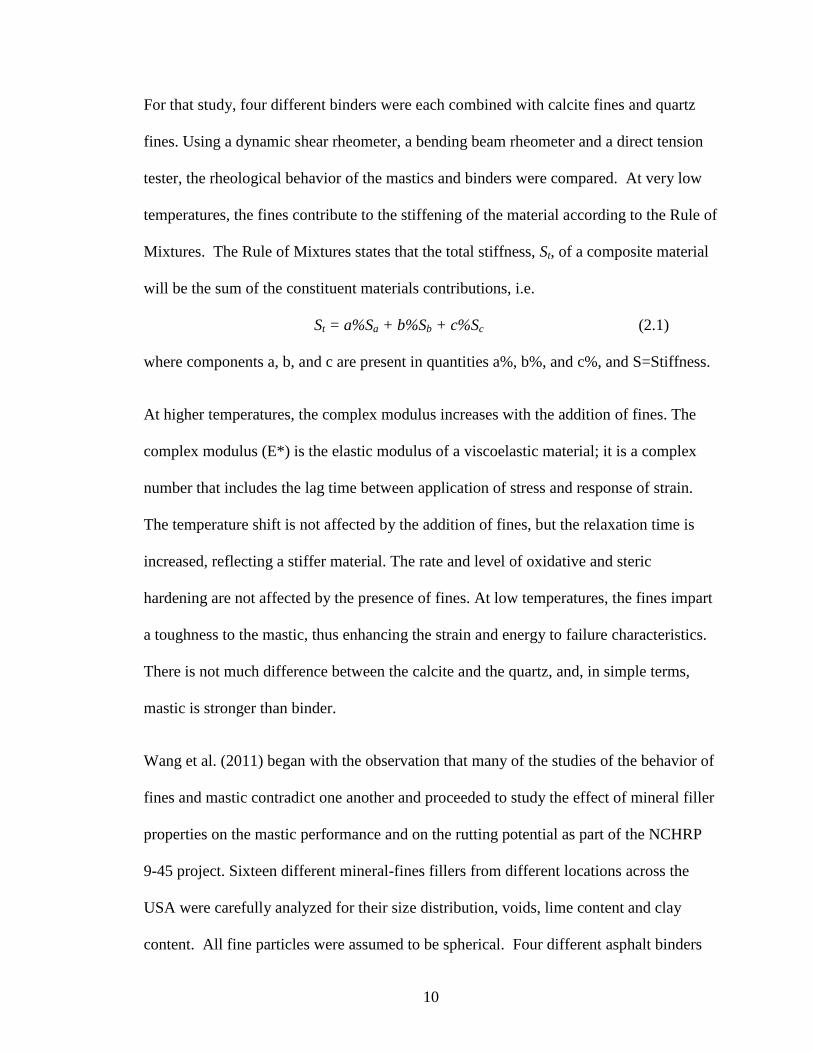
For that study, four different binders were each combined with calcite fines and quartz
fines. Using a dynamic shear rheometer, a bending beam rheometer and a direct tension
tester, the rheological behavior of the mastics and binders were compared. At very low
temperatures, the fines contribute to the stiffening of the material according to the Rule of
Mixtures. The Rule of Mixtures states that the total stiffness, St, of a composite material
will be the sum of the constituent materials contributions, i.e.
St = a%Sa + b%Sb + c%Sc (2.1)
where components a, b, and c are present in quantities a%, b%, and c%, and S=Stiffness.
At higher temperatures, the complex modulus increases with the addition of fines. The
complex modulus (E*) is the elastic modulus of a viscoelastic material; it is a complex
number that includes the lag time between application of stress and response of strain.
The temperature shift is not affected by the addition of fines, but the relaxation time is
increased, reflecting a stiffer material. The rate and level of oxidative and steric
hardening are not affected by the presence of fines. At low temperatures, the fines impart
a toughness to the mastic, thus enhancing the strain and energy to failure characteristics.
There is not much difference between the calcite and the quartz, and, in simple terms,
mastic is stronger than binder.
Wang et al. (2011) began with the observation that many of the studies of the behavior of
fines and mastic contradict one another and proceeded to study the effect of mineral filler
properties on the mastic performance and on the rutting potential as part of the NCHRP
9-45 project. Sixteen different mineral-fines fillers from different locations across the
USA were carefully analyzed for their size distribution, voids, lime content and clay
content. All fine particles were assumed to be spherical. Four different asphalt binders
11
were used, two unmodified, two modified. Comparing the viscosities of the different
mastic mixtures to the binders, it was observed that different fillers exhibit different
physical-chemical interactions with different binders. SBS polymer modified binder
showed the strongest reaction with most of the fillers. Dynamic modulus and flow
number testing resulted in the conclusions that voids and CaO (lime) contents have more
effect on rutting potential than other characteristics of fines, especially for the coarse
mixture.
Huang et al. (2007) investigated the performance characteristics of different mineral
types and content percentages of filler. Using three different mineral-fillers to make
mastics and HMA, the properties of indirect tensile strength and tensile toughness were
measured. Disks of the mastic were tested on a dynamic shear rheometer. The following
conclusions were made: increasing the filler content increased the indirect tensile
strength, but decreased the toughness index and retained tensile strength (stripping).
Kandhal et al. (1998) also conducted a study of multiple types of mineral fines mixed
with asphalt binders, but for the purpose of determining which tests that are performed on
aggregate fines actually predict the performance of the final HMA applied to the
roadway. Note was made of the fact that one reason for increasing the P200 portion of
the aggregate in the HMA mix is to comply with environmental standards limiting the
amount of dust that can be released. The final conclusions were that rutting (permanent
deformation) correlates with the D60 (this means that 60% of the material passes through
a sieve of size D) and Methylene Blue tests on P200. No test correlated with fatigue
cracking. Stripping correlates well with D10 and Methylene Blue test results.
12
The same year, two of the authors of this study published the NCHRP Report 405, which
was updated to NCHRP Report 557 in 2006 (Kandhal and Parker 1998, White et al.
2006).
None of these studies mentioned the existence of mica.
2.6 NCHRP Reports
NCHRP Report 405, in 1998, evaluated aggregate tests through a literature review and
some laboratory testing and issued a list of recommended tests for designing asphalt
pavement. At the time, it was recommended that more extensive testing be done,
especially field testing. This work was done and the follow-up report, NCHRP Report
557, was issued in 2006 (White et al. 2006).
Asphalt concrete is about 95% aggregate, by weight. About 6% of the aggregate weight
is made up of the P200 fines, which can be considered either an extender or a filler. The
amount and characteristics of the P200 fines can contribute to susceptibility to moisture
damage or fatigue cracking of an HMA mix. The Methylene Blue Test for p0.075
(AASHTO TP57) yields a value (MBV) that can be correlated to the stiffness of the
mastic. The higher the MBV, the stiffer the mastic as measured by Superpave Shear
Tests. This can, in turn be correlated to better rutting resistance, but low resistance to
fatigue cracking. The Report also recommends determining the D10 and D60 particle
sizes. It does not mention mica specifically at any point.
13
2.7 Aging
The aging of asphalt binders, whether in the field or during accelerated laboratory aging,
is a very complex process that has received considerable attention from researchers for
many years. It is generally agreed that the aging process occurs in two distinct steps: (1)
during construction (plant mixing, placement, and compaction) and (2) during the service
life of the pavement. This aging, in general, results in a change in the molecular size
distribution of an asphalt binder. Specifically, an increase in the molecular size which
results in an increase in the viscosity and stiffness of an asphalt binder. In the field, this
leads to a fragility and failure. (Lee et. al 2007)
During construction, the aging occurs at an elevated temperature, and there is opportunity
for the asphalt binder to both oxidize and to lose volatile compounds. In contrast, aging
during the service life of a pavement occurs at a much lower temperature where oxidation
is the primary aging mechanism. There is relatively little volatile compound loss during
the service life of a pavement. (Anderson and Bonaquist, 2012)
Hence, the two types of aging must be addressed separately for simulation in the
laboratory.
Short-term aging, that which occurs during construction, is simulated with the Rolling
Thin Film Oven (RTFO). In this test the asphalt binder is exposed to astream of air at
163C, which is representative of mixing and compaction temperatures.
For a pavement in the field, maximum service temperatures range from 58to 70C.
Research has shown that the aging mechanisms that occur in the laboratory during
simulated aging change significantly when the aging temperature rises above
approximately 110 oC.
14
While it is known that raising the temperature of an asphalt doubles the rate of oxidation,
the change that occurs at 110oC limits the extent to which temperature can be used to
accelerate the simulation of long-term aging. Also, the long-term aging mechanism, and
its associated kinetics, is more reliably simulated when the accelerated aging is conducted
as close as possible to the service temperature.
The Pressure Aging Vessel (PAV) is used to simulate long term aging of the pavement in
service for five to ten years. This device exposes the sample to 100oC at 2.1 MPa (almost
21 times higher than atmospheric pressure) for 20 hours. Convection oven aging has been
studied at various temperatures for various lengths of time. Yousefi (2010) studied the
aging of pure binders exposed to 100oC for 1 to 20 weeks. It was found that unmodified
binder shows steadily increasing stiffness. However, SB4% polymer modified binder
levels off after a week and ultimately shows only about 25% of the stiffness increase.
Lee et. al (2007) studied aging at 134 oC to 154
oC for 2 to 4 hours and found that the
aging was comparable to that inflicted by the RTFO.
The AASHTO standards written for the RTFO and PAV aging processes are designed for
pure binder, not for mastic.
2.8 XRD
X-ray diffraction (XRD) was developed in the early 1900’s as a method of identifying
crystals. Databases have been developed with the diffraction patterns of many crystals.
These diffraction patterns are used to identify crystals similar to the manner in which
fingerprints identify humans.
15
The atoms of a crystalline material are arranged in a regular, repeated pattern. Crystals
are highly ordered, three-dimensional structures. When an X-ray beam strikes such a
structure, it causes electrons in its path to vibrate with the same frequency as the incident
X-radiation. These vibrating electrons absorb some of the X-ray energy and, acting as a
source of new wave fronts, emit this energy as X-radiation of the same frequency and
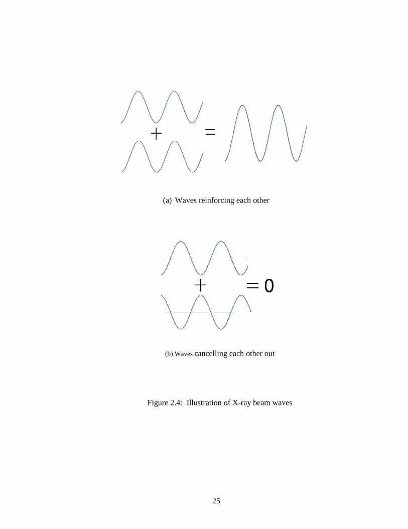
wave-length (Klein 1993). Usually, the waves interfere with one another and no
detectible beam is emitted. However, if the wavelength, frequency, crystal structure and
angle of incidence are right, the waves become in-phase, reinforce one another and result
in a beam that can be detected. Figures 2.4(a) and 2.4(b) illustrate the concept of waves
reinforcing and cancelling each other, respectively. It is this detected beam that serves to
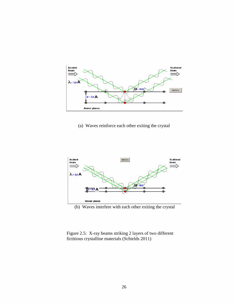
identify the crystal. Figure 2.5(a) shows an example of the wave patterns for a fictitious
crystal in which the exiting waves are in-phase and reinforce each other, resulting in a
detectible signal beam. Figure 2.5(b) shows an example of a different fictitious crystal
for which the combination of separation distance (d), wavelength and angle of incidence
result in interference in the exiting waves and there is no detectible signal out.
In order for the waves to reinforce one another, Braggs Law must be satisfied. That is:
(2.2)
where n is an integer, λ is the wavelength of the x-ray, d is the distance between the
parallel planes in the crystal and theta (θ) is the angle of incidence.
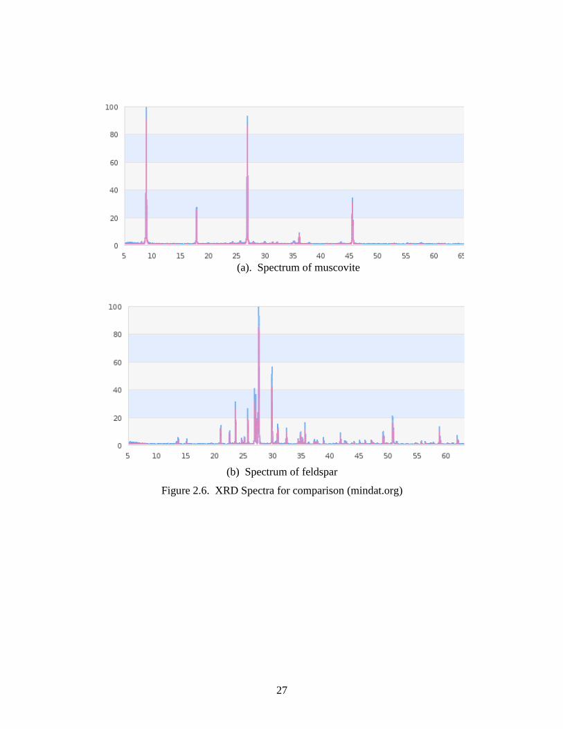
As each crystal has an identifying pattern of detectible beams, the patterns must be
compared to previously known patterns. Figures 2.6(a) and 2.6(b) show the XRD
patterns of muscovite and feldspar, respectively, aligned for comparison of the peak
16
locations. Muscovite shows strong peaks at 2theta equal to approximately 9 and 26
degrees, a medium peak at about 26 degrees, medium low peaks at about 17 and 46
degrees with several very weak peaks. Feldspar shows only one strong peak at 2theta
equal to 28 degrees, one medium peak at 30 degrees, medium low peaks at 24, 26, 27,
and 51 degrees, and many lower peaks. The only overlapping of peaks between feldspar
and muscovite is at 2theta equals 27 degrees.
2.9 SEM
The Scanning Electron Microscope (SEM) creates high-resolution visual images at very
high magnification. Included with the imaging function is the Energy Dispersive X-ray
(EDX) function, which analyzes the characterization x-ray emitted from a sample and
performs chemical element analysis on the surface of the sample.
The fundamental principals upon which the SEM is based were first discovered during
the 1930’s and the first commercial SEM was offered in 1965 (JEOL Ltd., 2006). The
machines have been improved and functionality broadened much since then.
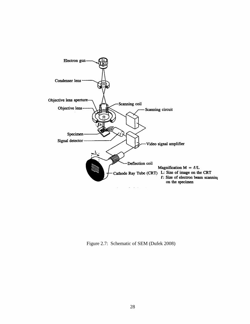
The basic concept behind the function of the SEM is as follows. A very fine beam of
electrons (only several nanometers wide) strikes the sample. This causes the electrons of
the sample to emit several different types of information: secondary electrons,
backscattered electrons, Auger electrons, X-rays and cathodo-luminescence. Each of
these is used for different types of observations; such as, secondary electrons are used to
observe the surface topography and X-rays are used to perform elemental analysis with
the EDX.
17
Current technology requires the sample to be electrically grounded to the machine, which
is achieved by depositing a very thin layer of graphite or gold on a non-conductive
sample with a vaporizing sputter coating machine. Because there is a strong vacuum in
the sample chambers of both the sputtering equipment and the SEM, the sample must be
prepared in such a way that neither the sample nor the equipment is damaged. The image
created by SEM is a very close up visual image. Hence, if there are no surface
deformations or features, the image shows blank. Figure 2.7 shows a schematic of the
SEM.
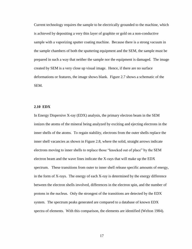
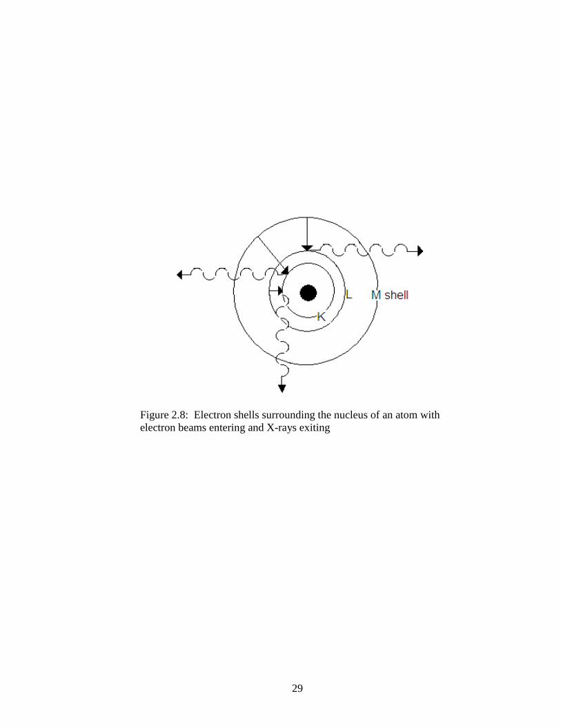
2.10 EDX
In Energy Dispersive X-ray (EDX) analysis, the primary electron beam in the SEM
ionizes the atoms of the mineral being analyzed by exciting and ejecting electrons in the
inner shells of the atoms. To regain stability, electrons from the outer shells replace the
inner shell vacancies as shown in Figure 2.8, where the solid, straight arrows indicate
electrons moving to inner shells to replace those “knocked out of place” by the SEM
electron beam and the wave lines indicate the X-rays that will make up the EDX
spectrum. These transitions from outer to inner shell release specific amounts of energy,
in the form of X-rays. The energy of each X-ray is determined by the energy difference
between the electron shells involved, differences in the electron spin, and the number of
protons in the nucleus. Only the strongest of the transitions are detected by the EDX
system. The spectrum peaks generated are compared to a database of known EDX
spectra of elements. With this comparison, the elements are identified (Welton 1984).
18
Welton (1984) writes that a large piece of muscovite showing a smooth, flat surface has
the EDX spectrum with following peaks: aluminum (Al) at 1.5 Kev, silicon (Si) at
1.75Kev and potassium (K) at 3.25 Kev in two peaks.
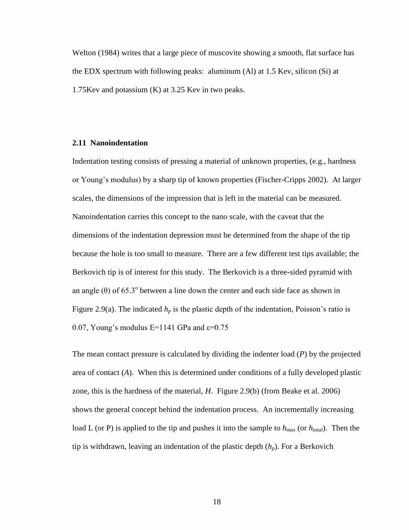
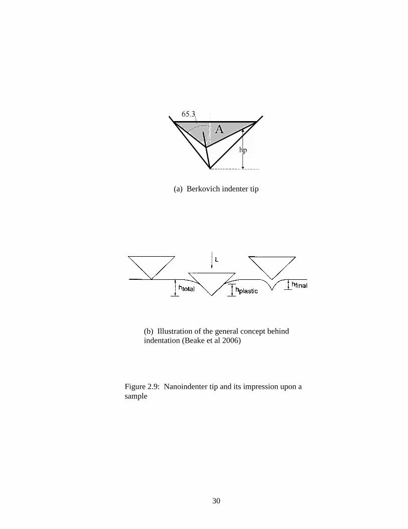
2.11 Nanoindentation
Indentation testing consists of pressing a material of unknown properties, (e.g., hardness
or Young’s modulus) by a sharp tip of known properties (Fischer-Cripps 2002). At larger
scales, the dimensions of the impression that is left in the material can be measured.
Nanoindentation carries this concept to the nano scale, with the caveat that the
dimensions of the indentation depression must be determined from the shape of the tip
because the hole is too small to measure. There are a few different test tips available; the
Berkovich tip is of interest for this study. The Berkovich is a three-sided pyramid with
an angle (θ) of 65.3o between a line down the center and each side face as shown in
Figure 2.9(a). The indicated hp is the plastic depth of the indentation, Poisson’s ratio is
0.07, Young’s modulus E=1141 GPa and ε=0.75
The mean contact pressure is calculated by dividing the indenter load (P) by the projected
area of contact (A). When this is determined under conditions of a fully developed plastic
zone, this is the hardness of the material, H. Figure 2.9(b) (from Beake et al. 2006)
shows the general concept behind the indentation process. An incrementally increasing
load L (or P) is applied to the tip and pushes it into the sample to hmax (or htotal). Then the
tip is withdrawn, leaving an indentation of the plastic depth (hp). For a Berkovich
19
indenter, the projected area, A, is determined using the plastic depth of penetration, hp,
using the equation:
(2.3)
Hence the hardness is:
(2.4)
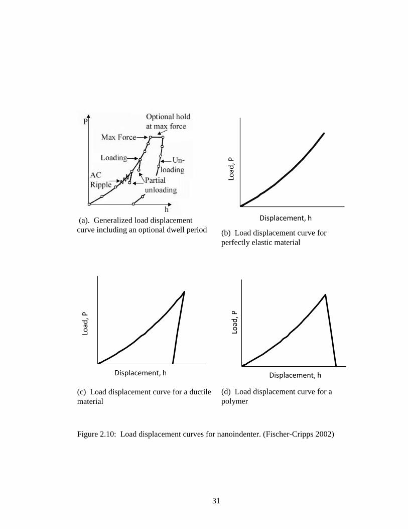
As the indenter tip, with known properties, is pressed into the sample of unknown
properties, and then withdrawn, the time, load required and depth of indentation is
constantly measured. A load-displacement plot is generated with depth of indentation on
the horizontal axis and force on the vertical axis.
Figure 2.10(a) shows a generalized curve that includes a dwell time. Examples of curves
for perfectly elastic, ductile (elastic-plastic), and polymer (visco-elastic) are shown in
Figure 2.10(b), 2.10(c) and 2.10(d), respectively. The polymer curve shows the
displacement due to creep.
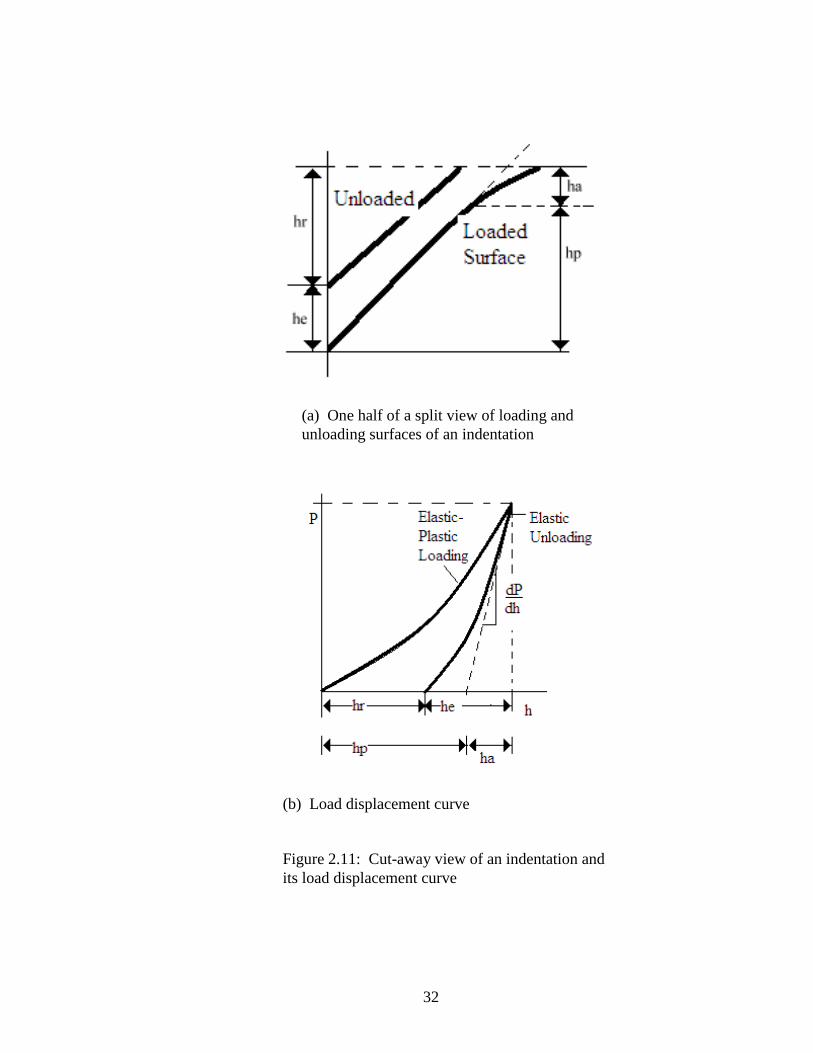
Figure 2.11(a) illustrates a dissection of surfaces created in an elastic-plastic material
resulting from the insertion and withdrawal of the indenter tip and 2.11(b) shows the
load-displacement curve reflecting it. The dimensions shown are: hp (sometimes referred
to as h intercept) is the plastic depth, or the anticipated depth of total penetration minus
the elastic recovery if the slope of the unloading curve was constant, he is the elastically
recovered depth after the load is removed, hr is the residual depthof the impression left by
the indenter, and ha is the depth from the edge of the contact area to the surface of the
sample.
20
According to Fisher-Cripps (2002), a reduced modulus, Er, has been defined. It is
calculated from the slope of the top portion of the unloading curve, where the response is
most elastic, using Eq. 2.5.
(2.5)
where β is a correction factor equal to 1.034 for a Berkovich indenter and
The stiffness, S, is calculated using the Oliver and Pharr method of power-law fitting
(Beake et al. 2006). From Er, Young’s modulus, Es, can be determined with Eq. 2.6
(Tarefder, et al. 2010).
(2.6)
where s is for sample, i is for indenter, E is Young’s modulus and ν is Poisson’s ratio.
For the Berkovich tip, Ei =1141 GPa and ν= 0.07. For asphaltic materials, ν=0.4.
While much nanoindentation work has been done with harder (more elastic) materials in
the last decades, very little has been done with asphalt binders. Tarefder et al. (2008)
succeeded in identifying the separate phases of asphalt, i.e.: binder, mastic, matrix and
rock in samples of asphalt concrete. Yousefi (2010) had success analyzing thin films of
binder on glass slides. There is no standardized method of preparing asphalt materials for
nanoindentation.
21
2.12 Bending Beam Rheometer
The Bending Beam Rheometer (BBR) has been used for several decades to test asphalt
binders at low temperatures to determine their susceptibility to thermal cracking. This
type of cracking occurs on roadways as the asphalt pavement shrinks in cold
temperatures (Roberts et al. 1991). It may happen in one cycle down to an extremely
cold temperature or after several cycles of heating and cooling to more moderate
temperatures. AASHTO Test T 313-08 describes the detail of the test precisely.
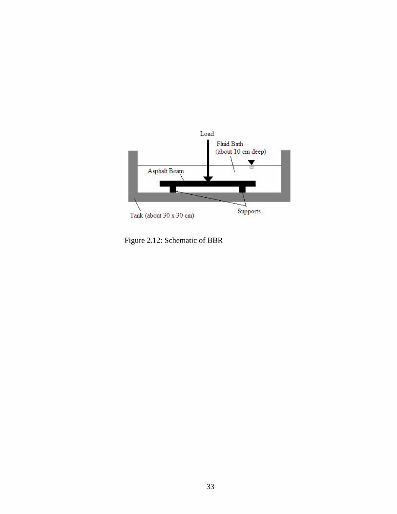
Figure 2.12 shows a schematic of the very basic part of the test setup. A beam of asphalt
is simply supported in a bath of cold fluid. The beam is made to very specific dimensions
(125 x 6.25 x 12.5 mm) and kept in the cold bath for one hour before testing. A load,
nominally 980 mN, is applied at the center of the beam for 240 seconds and the
deflection of the beam is measured continuously. The creep stiffness, S(t), of the beam is
calculated with Eq. 2.7:
(2.7)
where S(t)=creep stiffness at time, t=60 seconds, P=applied load, 980 mN, L=distance
between supports, 102 mm, b=beam width, 12.5 mm, h=beam thickness, 6.25 mm,
δ(t)=deflection at time, t=60 seconds. AASHTO T 313 requires the beam to be 6.35 mm
thick and 12.7 mm wide.
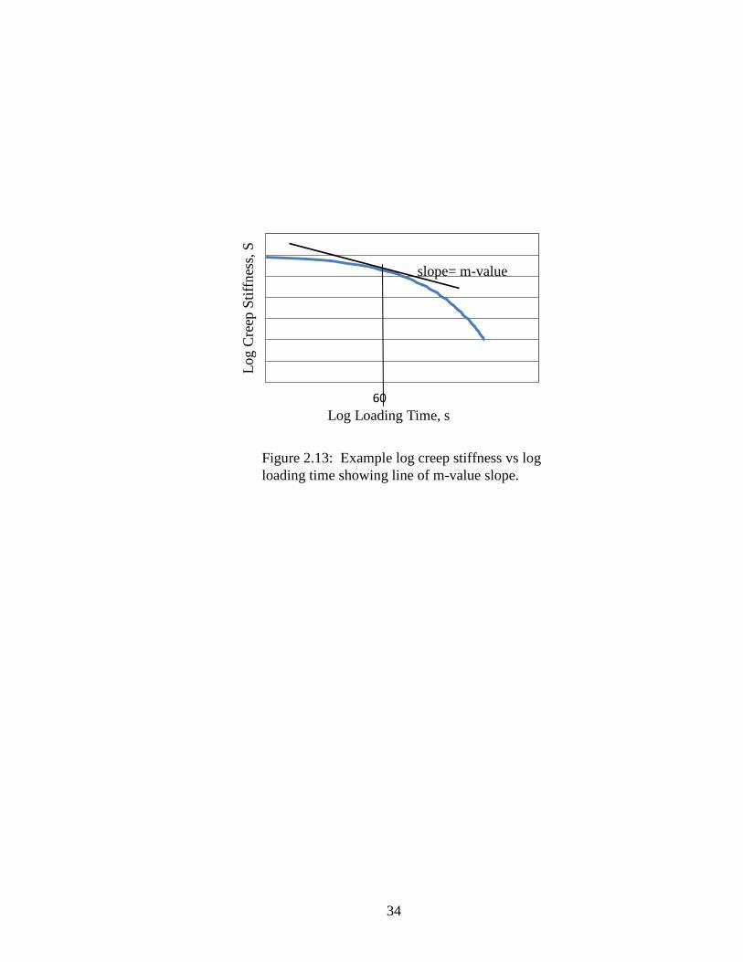
Modern BBR equipment automatically calculates the creep stiffness and m-value, where
m-value is the slope of the curve of Log Creep Stiffness vs. Log Loading Time at t=60
seconds. Figure 2.13 shows an example of the curve and the m-value tangent line.
22
.
Figure 2.1. Specimen of muscovite (Courtesy
University of New Mexico Earth and Planetary
Sciences Geology Museum)
23
Figure 2.2. Paper model of muscovite mineral (Courtesy University of
New Mexico Earth and Planetary Sciences Geology Museum)
24
Figure 2.3. Paper model of quartz mineral (Courtesy University of
New Mexico Earth and Planetary Sciences Geology Museum)
25
(a) Waves reinforcing each other
(b) Waves cancelling each other out
Figure 2.4: Illustration of X-ray beam waves
26
(a) Waves reinforce each other exiting the crystal
(b) Waves interfere with each other exiting the crystal
Figure 2.5: X-ray beams striking 2 layers of two different
fictitious crystalline materials (Schields 2011)
27
(a). Spectrum of muscovite
(b) Spectrum of feldspar
Figure 2.6. XRD Spectra for comparison (mindat.org)
28
Figure 2.7: Schematic of SEM (Dufek 2008)
29
Figure 2.8: Electron shells surrounding the nucleus of an atom with
electron beams entering and X-rays exiting
30
(b) Illustration of the general concept behind
indentation (Beake et al 2006)
Figure 2.9: Nanoindenter tip and its impression upon a
sample
(a) Berkovich indenter tip
31
(d) Load displacement curve for a
polymer
1
0
Load
, P
Displacement, h
(a). Generalized load displacement
curve including an optional dwell period
(b) Load displacement curve for
perfectly elastic material
1
0
Load
, P
Displacement, h
(c) Load displacement curve for a ductile
material
1
0 1 2 3
Load
, P
Displacement, h
Figure 2.10: Load displacement curves for nanoindenter. (Fischer-Cripps 2002)
32
(a) One half of a split view of loading and
unloading surfaces of an indentation
(b) Load displacement curve
Figure 2.11: Cut-away view of an indentation and
its load displacement curve
33
Figure 2.12: Schematic of BBR
34
Figure 2.13: Example log creep stiffness vs log
loading time showing line of m-value slope.
200
300
400
500
600
700
800
900
10 100 1000
Log C
reep
Sti
ffnes
s, S
Log Loading Time, s
slope= m-value
60
35
CHAPTER 3
METHODOLOGY
3.1 Mica
Mica for the following experiments was dug out of the earth in the forest wilderness
between the village of Petaca, New Mexico and the Apache II mica mine in Taos County,
New Mexico (see map, Figure 3.1).
As the mica was acquired in its natural state, cleaning was required. As it was handled
during cleaning, much of it fell apart in thin flakes quickly. Some of it held together
tightly as thick plates. Most of it fell into sheets less than 1 mm thick. These pieces
tended to stick together when wet. They all tended to adhere flat against the sides of any
mixing bowl, rendering them inaccessible to the mixing blades. As such, the grinding
methods chosen for processing involved gravity feed.
The mica was washed and rinsed several times with tap water to remove dirt and mold.
A final rinse with de-ionized water was done to remove minerals left by the tap water.
The mica was cut into pieces smaller than ½ inch square using scissors and a cork-screw
style food grinder. These pieces were placed in a kitchen blender and ground to a fine
powder. This powder was then sieved and the portion passing through the #200 sieve
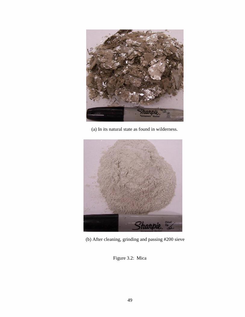
(P200) was used in the experiments for this study. Figure 3.2(a) shows the mica in its
native state. Figure 3.2(b) shows it after cleaning and grinding.
36
In the following sections, the mineral filler, excluding the mica, is referred to as “fines”.
The fines used in the experiments were obtained by sieving the P200 fines portion from
commercially available, oven dried “crusher fines” and ½″ aggregate obtained from
Lafarge Albuquerque. Care was taken to ensure that all of the fines in each set of
samples came from the same source. The asphalt binder used in the experiments was PG
58-28. The binder and the styrene-butadyene (SB) polymer were both collected from
Holly Asphalt of Albuquerque.
3.2 XRD
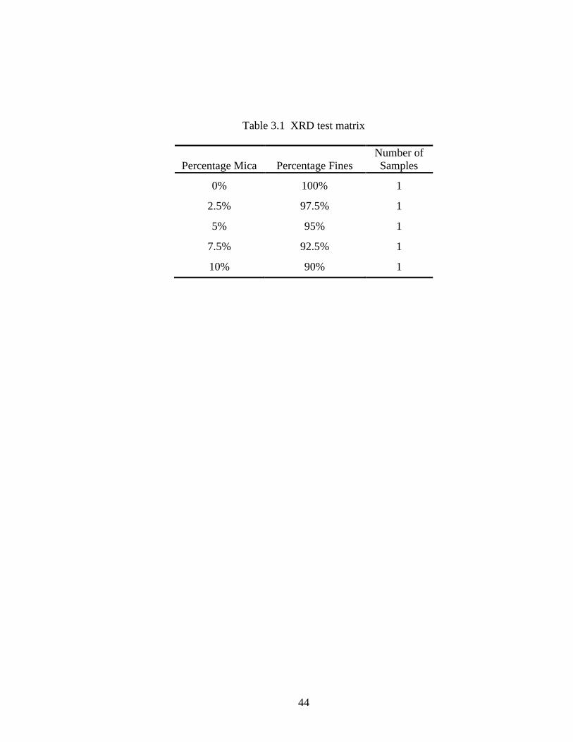
Samples for X-ray diffraction analysis were made by mixing fines with mica in varying
ratios, measured by weight. The sample test matrix is shown in Table 3.1. About 1/2
gram of each mica-fines mix was placed on its own glass slide. A few drops of de-
ionized water were added to each slide and each was mixed to create a slurry that coated
the slide. The water was allowed to evaporate, leaving the mica-fines mixes stuck to the
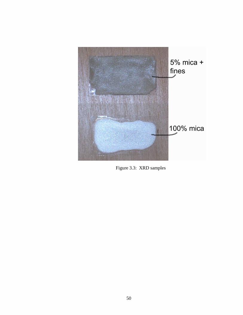
glass in thin, even coatings. Figure 3.3 shows two XRD samples. The top sample has
5% mica in fines. The bottom sample is pure mica. It was noted, during sample
preparation, that some particles floated to the surface of the water placed on the slide.
These particles settled on the surface of the sample as the water dried. It could not be
determined whether the floating particles were mica. If they were mica, then the surface
of the sample could skew the percentage of mica content. Also, as it is important to coat
the entire slide, the slurry was pushed very close to the edge. If the water went over the
edge of the slide, surface tension would pull all the floating particles off the slide, and the
whole process had to be done over.
37
Powdered samples were analyzed by X-ray diffraction (XRD) in the XRD Laboratory in
the Department of Earth and Planetary Sciences at the University of New Mexico, using a
Scintag Pad V diffractometer with DataScan 4 software (from MDI, Inc.) for system
automation and data collection. Cu-K-alpha radiation (40 kV, 35 mA) was used with a
Bicron Scintillation detector (with a pyrolitic graphite curved crystal monochromator).
Data were analyzed with Jade Software (from MDI, Inc.) using the International Center
for Diffraction Data (ICDD) PDF4 database for phase identification.
3.3 Mixing & Molding Mastic
Mastics were mixed using asphalt binder, SB polymer, fines and mica. The fines were
mixed with mica to make mixtures of 0%, 2.5%, 5%, 7.5% and 10% mica, by weight.
Many experiments were performed to determine how much asphalt binder should be
mixed with the mica-fines to achieve mastics which had high enough binder content to
make them workable enough to allow for repeatable experiments and high enough fines
content to insure that it was the fines portion, not the binder, that was being tested. It was
determined that each group of tests would require a different percentage of binder, but all
would be between 19% and 25%. This was of particular concern as much of this study
was focused on micro and nanoscale properties.
For SEM samples, mastics made from unmodified PG58-28 binder were mixed with 21%
binder and the five different concentrations of mica. The differences between the five
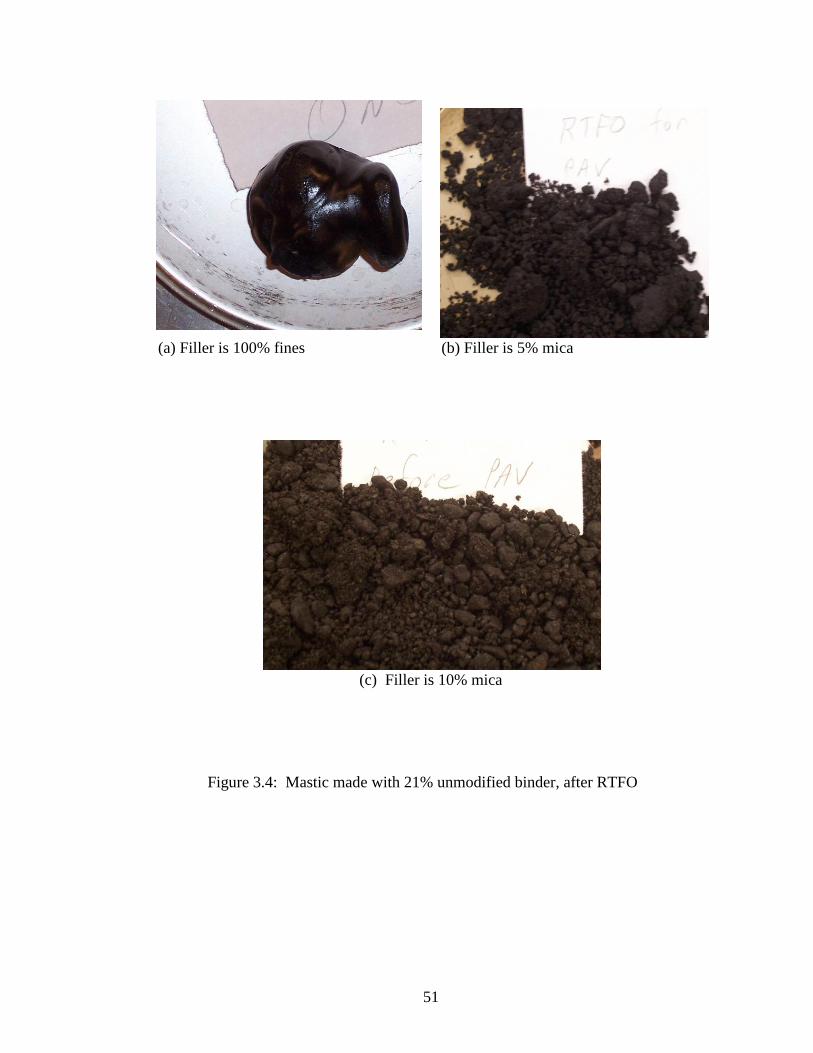
mixes were dramatically evident at the mixing stage. The 0% and 2.5% mica mixes were
far too rich and the 10% was rather dry. This can be seen in Figure 3.4(a), Figure 3.4 (b)
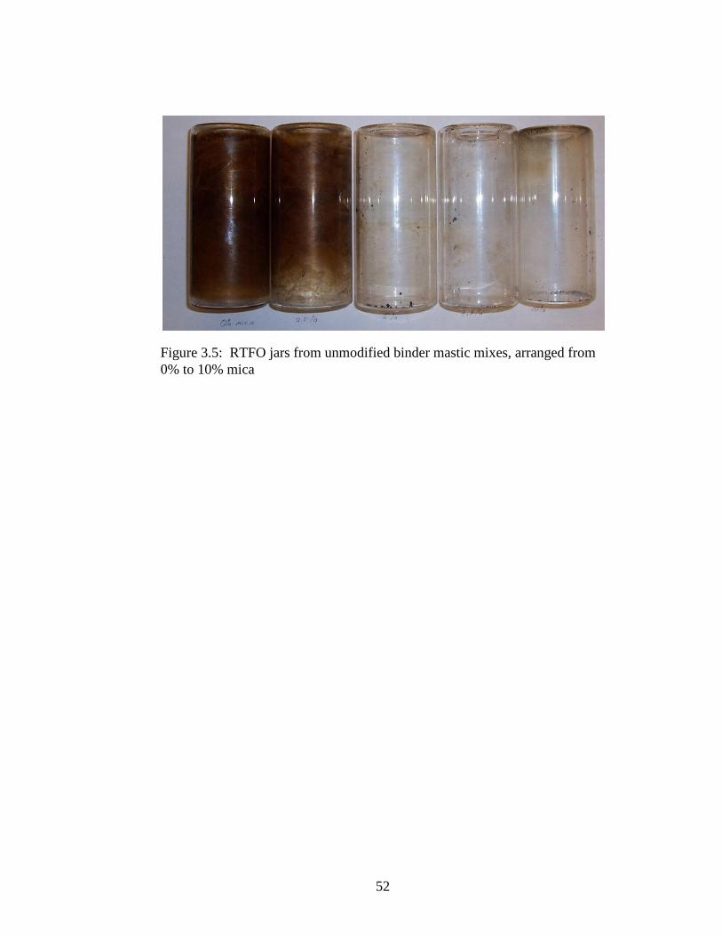
and Figure 3.4 (c) which show them after 85 minutes in the RTFO. Figure 3.5 is a
38
photograph of the RTFO jars after the five mixes had been short term aged. It illustrates
the same phenomenon as the 0% mica left a large amount of binder residue and the 10%
mica left the RTFO jar clean. It was difficult to pack the 7.5% and 10% mica mixes into
the molds as the volume of the mastic was greater, even though the weight was the same.
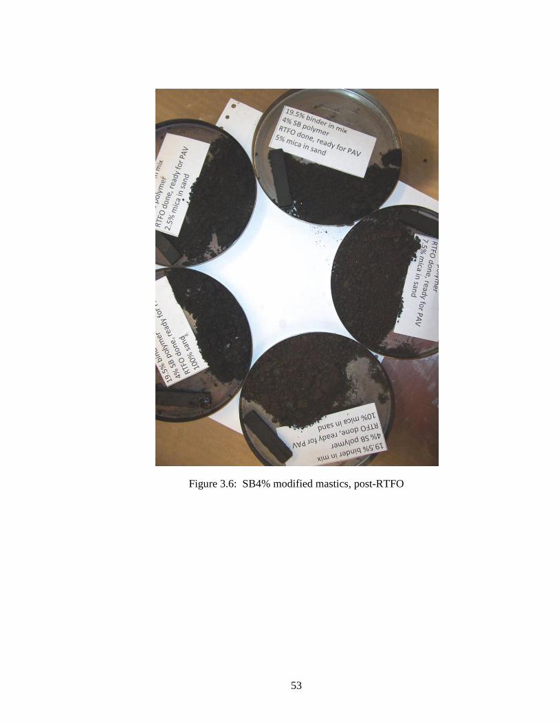
The percentage of binder was reduced for the SB4% modified mastics. The first attempt
used 19% binder, but that proved to be inadequate even for the 100% fines sample, so the
final mix had 19.5% binder. After RTFO, is was evident that the 0 and 2.5% samples
were rich enough for easy handling, but the 5, 7.5 and 10% samples were quite dry. All
five mixes are shown in Figure 3.6 where the 0% mica mix is obviously deep black and
sticking together while the 10% mica mix is brown and granular. The RTFO jars were all
clean after the cycle was run because these mastics left no residue. While dry, these
samples were considered to be adequately useable.
The mastics thus created were then subjected to various aging processes, according to the
matrices shown in Table 3.2(a) and Table 3.2(b). Each mix was 150 grams, from which
all the sample sticks were made. The aged mastics were compacted into molds yielding
sticks 0.5 x 0.125 x 2.12 inches (volume of 2.18 cm3) with 9 to 10 grams of mastic in
each, ensuring a density of about 4.4 g/cm3. The molds and tampers were heated to
325oF to aid the compaction process. The molds were coated with corn oil as a mold-
release agent before the mastic was put in. AASHTO T240 and R 28 were referenced for
the operation of the RTFO and PAV to the extent applicable. The standards are written
for binder alone, not for mastic. Oven aging consisted of 24 hours in a convection oven
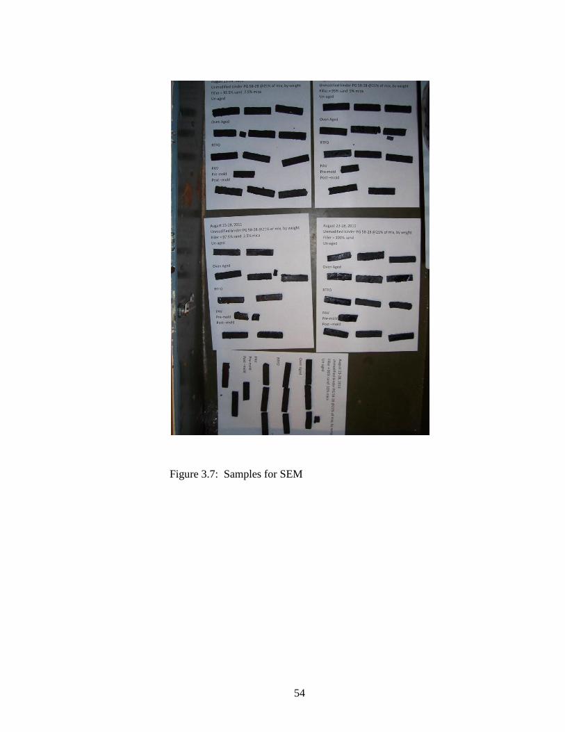
at 100oC. Figure 3.7 shows all the samples made with the unmodified binder mastics.
39
The issue of the mica absorbing more binder than the fines cannot be emphasized
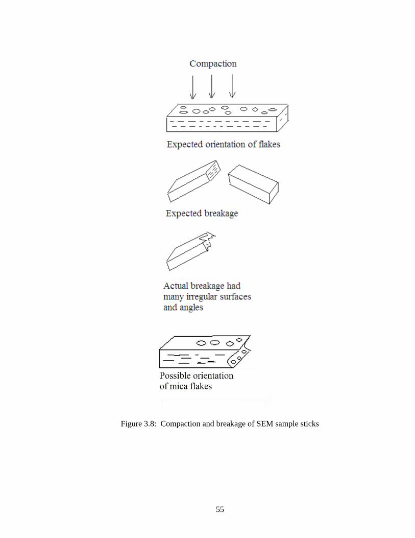
enough. It affected every aspect of the mixing, molding and handling of the samples.
The sample sticks with low percentages of mica were difficult to break at room
temperature, as they tended to deform in the grip and pull of the pliers. These samples
were put in the freezer to stiffen for about five minutes. They still tended to break at
irregular angles; as illustrated in Figure 3.8
3.4 SEM Sample Preparation
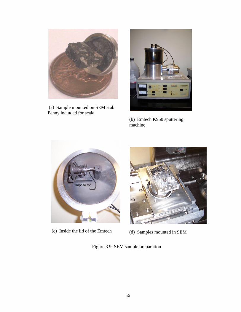
A small piece was broken off the end of a stick of each mastic mix. The broken pieces
were then placed on the SEM sample platforms (called stubs) with the broken face
exposed, as shown in Figure 3.9(a). The sample was attached to the stub with tape that is
electrically conductive and sticky enough to prevent the vacuum in the Emitech from
pulling the sample off the stub. The sample was carbonized with the Emitech sputtering
machine shown in Figure 3.9(b) to provide an electrical grounding path from the sample
to the body of the SEM. Figure 3.9(c) shows the inside of the lid of the Emitech and the
graphite rod that is vaporized and deposited on the sample in the process. The sharpness
and placement of the graphite rod in the lid is critical to controlling the amount of
graphite deposited on the sample. If the sample was not sufficiently grounded to the stub,
the electron beam would cause a charge to build up on the sample and the image would
be obscured with white lines of electronic noise. If too much graphite was deposited, the
detail of the surface features would be obscured. Figure 3.9(d) shows the samples
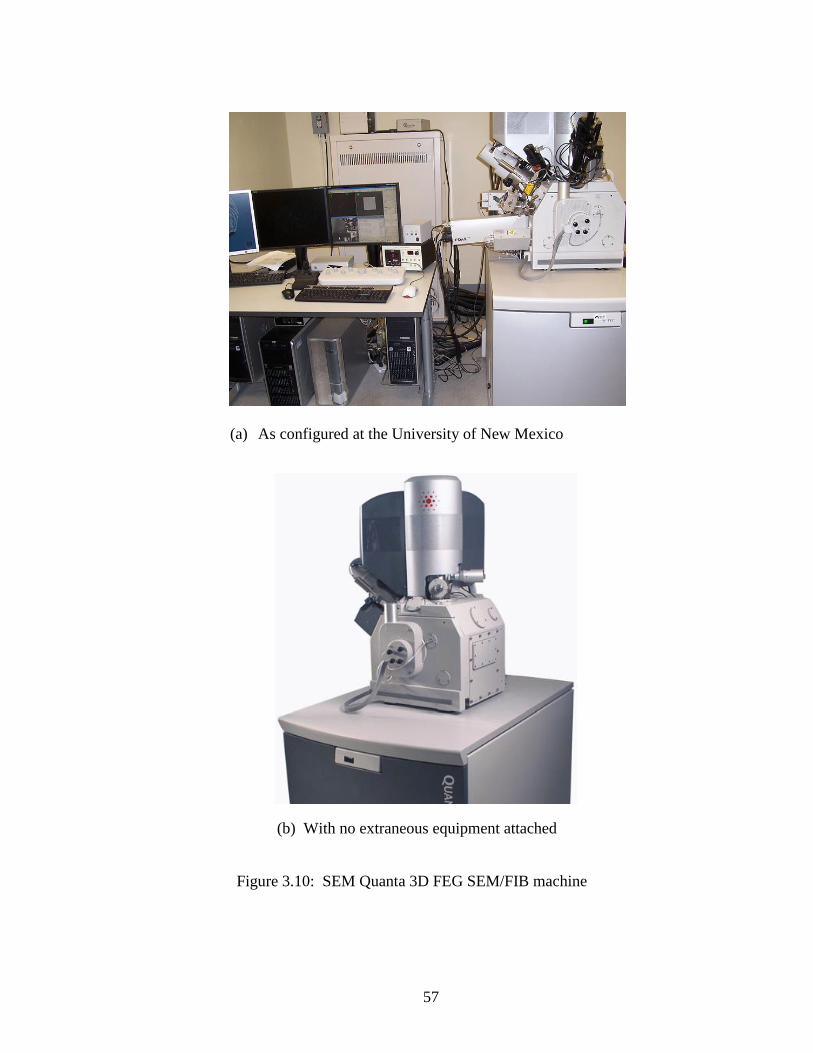
mounted inside the drawer of the SEM. Figure 3.10(a) shows the Quanta 3D FEG
40
SEM/FIB machine as it is configured at the University of New Mexico, equipped with
EDX using Genesis software, with three computers where the SEM work was done.
Figure 3.10(b) shows the SEM without the extra machinery (Dufek 2008).
3.5 Nanoindentation
Tests were performed using a MicroMaterials Ltd nanoindenter (Wrexham, UK.) A
three-sided pyramidal Berkovich tip with a semiangle of 65.27o was used.
As previous researchers had met with little success indenting unmodified binder, the bulk
of the nanoindentation done in this study used the binder modified with SB4% (Tarefder
et al. 2008, Yousefi 2010). The mastic sticks molded for the SEM experiments provided
the material for the nanoindentation samples. The first experiment was done on only
three samples made unmodified binder, post-PAV, 5 indentations each to establish where
to start with test parameters. The second experiment was more thorough, with 5 mica
concentrations tested at 2 age levels for a total of 10 samples receiving 10 indentations
each. Tables 3.3(a) and 3.3(b) show the test matrices applied.
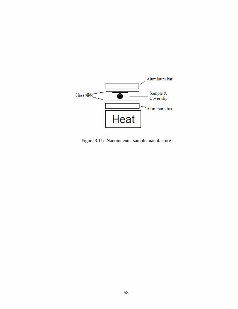
Mastic samples were mounted on glass slides in the following method, keeping
somewhat close to procedures used in previous studies of asphalt binder (Yousefi 2010).
The glass slides were cleaned with ethanol. A half inch square was marked with a fine
point permanent marker on each slide. A clean, smooth piece of flat aluminum bar was
placed on a hot plate that was maintained at 220oF to 250
oF. The glass slide was placed
on the aluminum bar. About 0.25 grams of mastic was placed on the slide in the square.
A plastic cover slip, cut from the strips used in BBR mold preparation, was placed over
the mastic. Another clean glass slide was placed on top of that. Another aluminum bar,
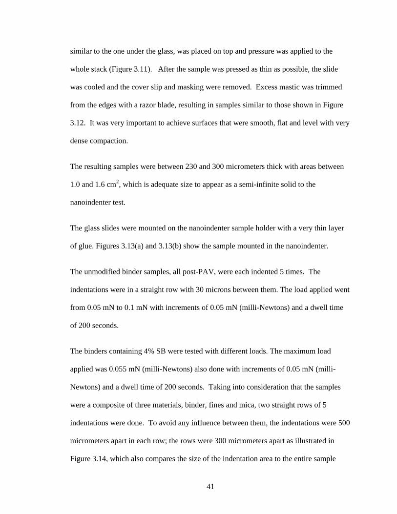
41
similar to the one under the glass, was placed on top and pressure was applied to the
whole stack (Figure 3.11). After the sample was pressed as thin as possible, the slide
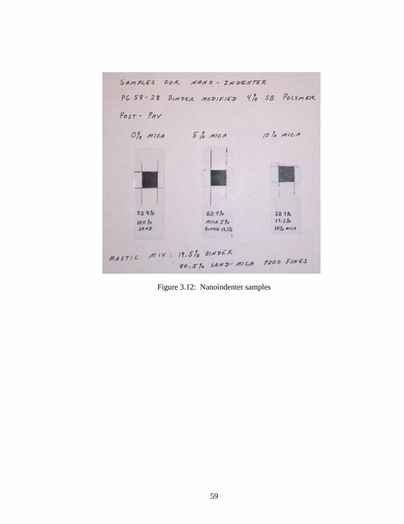
was cooled and the cover slip and masking were removed. Excess mastic was trimmed
from the edges with a razor blade, resulting in samples similar to those shown in Figure
3.12. It was very important to achieve surfaces that were smooth, flat and level with very
dense compaction.
The resulting samples were between 230 and 300 micrometers thick with areas between
1.0 and 1.6 cm2, which is adequate size to appear as a semi-infinite solid to the
nanoindenter test.
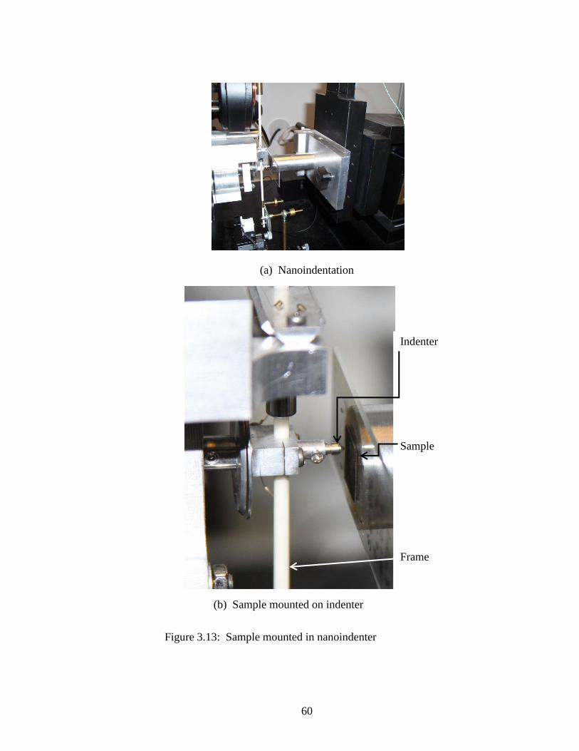
The glass slides were mounted on the nanoindenter sample holder with a very thin layer
of glue. Figures 3.13(a) and 3.13(b) show the sample mounted in the nanoindenter.
The unmodified binder samples, all post-PAV, were each indented 5 times. The
indentations were in a straight row with 30 microns between them. The load applied went
from 0.05 mN to 0.1 mN with increments of 0.05 mN (milli-Newtons) and a dwell time
of 200 seconds.
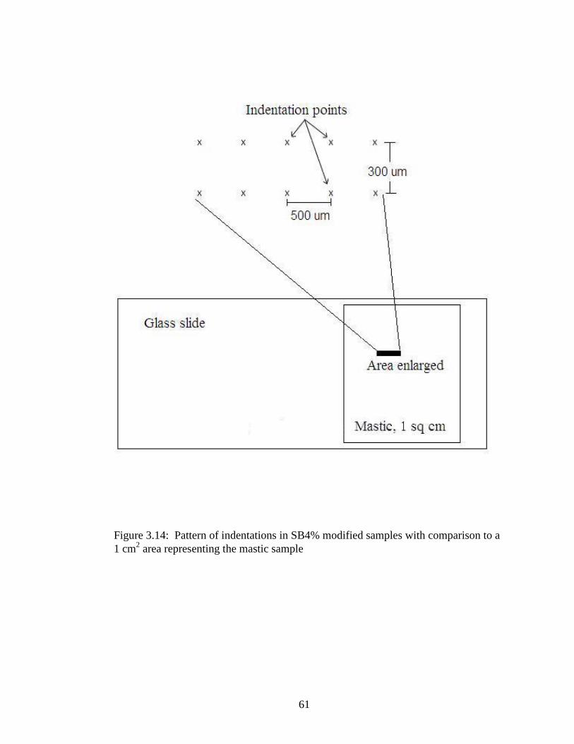
The binders containing 4% SB were tested with different loads. The maximum load
applied was 0.055 mN (milli-Newtons) also done with increments of 0.05 mN (milli-
Newtons) and a dwell time of 200 seconds. Taking into consideration that the samples
were a composite of three materials, binder, fines and mica, two straight rows of 5
indentations were done. To avoid any influence between them, the indentations were 500
micrometers apart in each row; the rows were 300 micrometers apart as illustrated in
Figure 3.14, which also compares the size of the indentation area to the entire sample
42
size. This also decreased the likelihood that one mica flake would be hit by two
indentations.
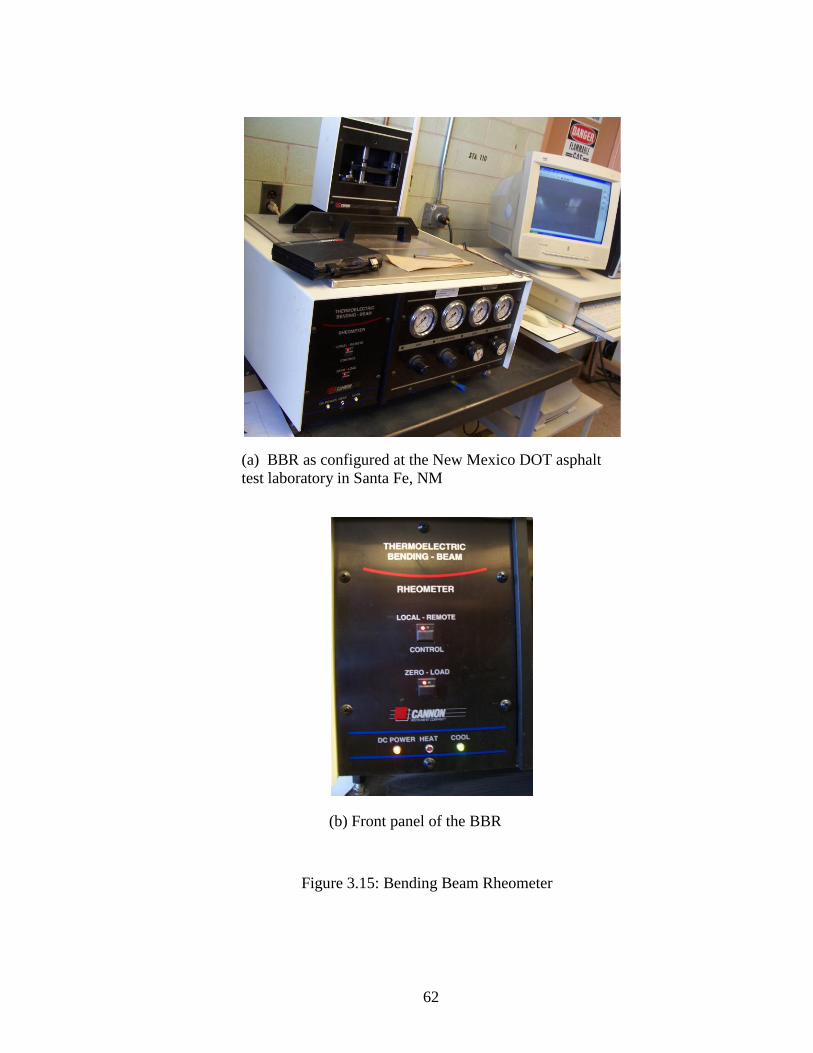
3.6 Bending Beam Rheometer (BBR)
BBR tests were performed at the asphalt binder test laboratory of the New Mexico State
Department of Transportation located in Santa Fe, NM. The machine used was a
Thermoelectric Cannon, shown in Figures 3.15(a) and 3.15(b). To the extent that
AASHTO T 313-08, Determining the Flexural Creep Stiffness of Asphalt Binder Using
the Bending Beam Rheometer (BBR), could be applied to a mastic, it was followed.
Samples for the BBR were prepared in a manner very similar to the SEM samples.
However only three concentrations of mica in fines were prepared, a larger percentage of
binder was mixed in the mastic to enable easier handling and the sample beams were
bigger. The nature of the BBR test requires considerable precision in size and
homogeneity of the sample. The mastics tested in this experiment were made with binder
modified with 4% SB polymer. Table 3.4 shows the test matrix used for the experiment.
In separate containers, fines were mixed with mica concentrations of 0%, 5% and 10%.
These mixes were then made into mastics with 21% binder. As the mixing of the mica-
fines requires an extended time to mix into the binder evenly, particularly the modified
binder, great care was taken to prevent over-heating. After many experiments, it was
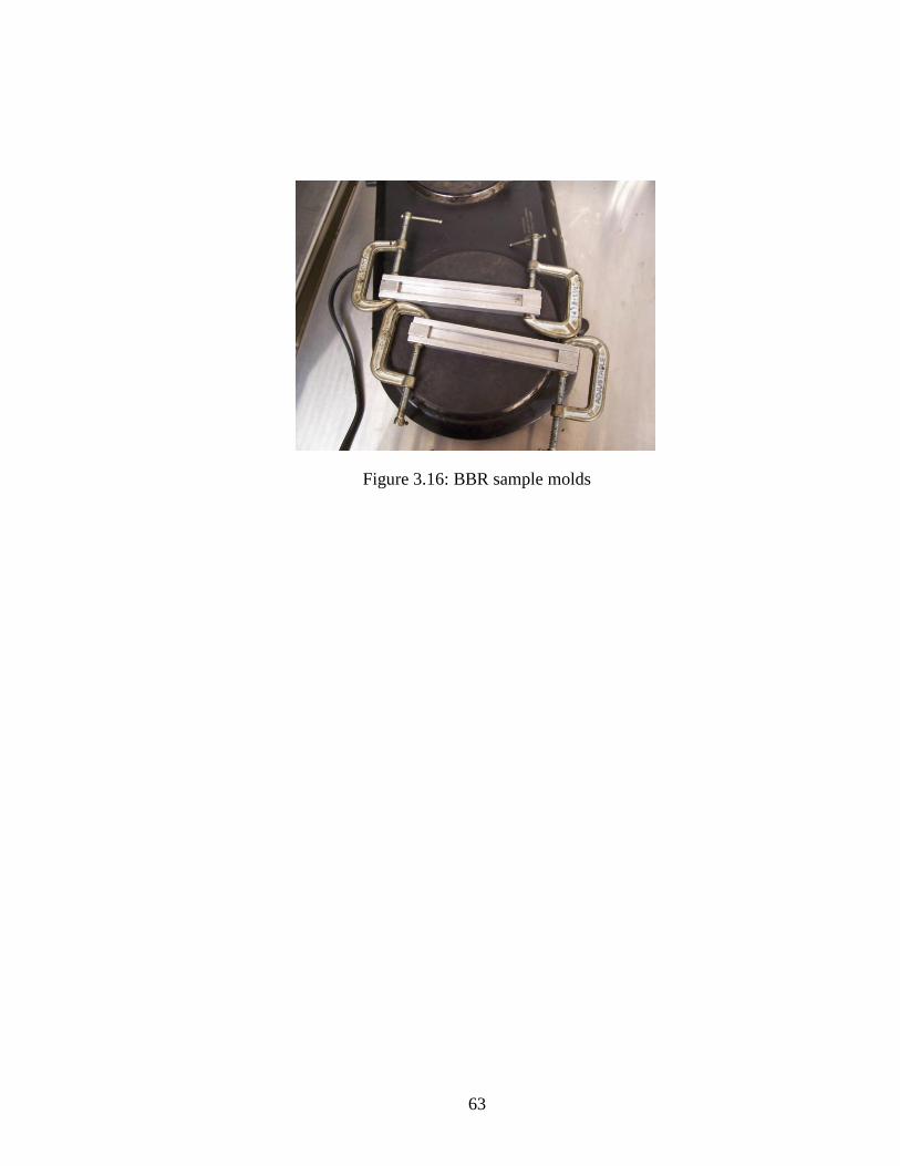
determined that the beams could be consistently made with a weight of 20-21 grams. For
the actual manufacture of the samples, 21 grams of mastic was pre-weighed and
compacted into the molds shown in Figure 3.16. These are standard BBR test sample
43
molds, held together with metal clamps instead of rubber bands. Also shown in Figure
3.16 is the hotplate which was used to maintain the mold temperature near 325oF. A
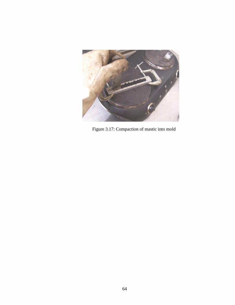
mixture of glycerin and talcum powder was used as a mold release agent. As some
mastic inevitably was spilled during the compacting effort, the samples actually weighed
20.5 +/- 0.4 grams each. In length and width they measured very close to the dimensions
required by AASHTO T 313-08 (125 x 12.5 mm), however there was some variation on
the depth dimension which should be 6.25. The samples measured 6.76 +/- 0.86 mm.
As required by AASHTO T 313-08, the samples were kept in the cold bath for 60
minutes +/- 5 minutes before testing. The BBR test was run normally.
44
Table 3.1 XRD test matrix
Percentage Mica
Percentage Fines
Number of
Samples
0% 100% 1
2.5% 97.5% 1
5% 95% 1
7.5% 92.5% 1
10% 90% 1
45
Table 3.2(a) SEM test matrix for unmodified binder mastic
Unmodified
Binder Mix Unaged Oven Aged RTFO
RTFO + PAV
Pre-molded
RTFO + PAV
Post-molded
100% fines 1 1 1 1 1
2.5% mica 1 1 1 1 1
5% mica 1 1 1 1 1
7.5% mica 1 1 1 1 1
10% mica 1 1 1 1 1
Table 3.2(b) SEM test matrix for SB4% modified binder mastic
SB 4%
Binder Mix
Unaged Oven Aged RTFO RTFO + PAV
Pre-molded
RTFO + PAV
Post-molded
100% fines 1 1 1 1 1
2.5% mica 1 1 1 1 1
5% mica 1 1 1 1 1
7.5% mica 1 1 1 1 1
10% mica 1 1 1 1 1
46
Table 3.3(a) Nanoindenter test matrix, unmodified binder mastic
% Mica in
aggregate fines
Aged with RTFO and
PAV
0 5 indentations
5 5 indentations
10 5 indentations
Table 3.3(b) Nanoindenter test matrix, SB4% modified binder mastic
% Mica in
aggregate fines
Aged with RTFO Aged with RTFO
and PAV
0 10 indentations 10 indentations
2.5 10 indentations 10 indentations
5 10 indentations 10 indentations
7.5 10 indentations 10 indentations
10 10 indentations 10 indentations
47
Table 3.4 BBR test matrix for SB4% binder mastic
SB 4%
Binder Mix
Unaged Oven Aged RTFO RTFO + PAV
100% fines 2 bars 2 bars 2 bars 2 bars
5% mica 2 bars 2 bars 2 bars 2 bars
10% mica 2 bars 2 bars 2 bars 2 bars
48
Figure 3.1: BLM(2006) map of wilderness area where mica was acquired
49
Figure 3.2: Mica
(a) In its natural state as found in wilderness.
(b) After cleaning, grinding and passing #200 sieve
50
Figure 3.3: XRD samples
51
(a) Filler is 100% fines (b) Filler is 5% mica
(c) Filler is 10% mica
Figure 3.4: Mastic made with 21% unmodified binder, after RTFO
52
Figure 3.5: RTFO jars from unmodified binder mastic mixes, arranged from
0% to 10% mica
53
Figure 3.6: SB4% modified mastics, post-RTFO
54
Figure 3.7: Samples for SEM
55
Figure 3.8: Compaction and breakage of SEM sample sticks
56
(b) Emtech K950 sputtering
machine
(a) Sample mounted on SEM stub.
Penny included for scale
(c) Inside the lid of the Emtech
(d) Samples mounted in SEM
Figure 3.9: SEM sample preparation
57
(a) As configured at the University of New Mexico
(b) With no extraneous equipment attached
Figure 3.10: SEM Quanta 3D FEG SEM/FIB machine
58
Figure 3.11: Nanoindenter sample manufacture
59
Figure 3.12: Nanoindenter samples
60
(a) Nanoindentation
(b) Sample mounted on indenter
Figure 3.13: Sample mounted in nanoindenter
Indenter
Sample
Frame
61
Figure 3.14: Pattern of indentations in SB4% modified samples with comparison to a
1 cm2 area representing the mastic sample
62
(a) BBR as configured at the New Mexico DOT asphalt
test laboratory in Santa Fe, NM
(b) Front panel of the BBR
Figure 3.15: Bending Beam Rheometer
63
Figure 3.16: BBR sample molds
64
Figure 3.17: Compaction of mastic into mold
65
CHAPTER 4
SEM ANALYSIS OF MASTIC MICA
4.1 Introduction
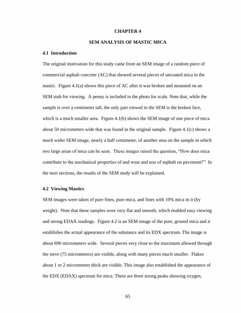
The original motivation for this study came from an SEM image of a random piece of
commercial asphalt concrete (AC) that showed several pieces of uncoated mica in the
mastic. Figure 4.1(a) shows this piece of AC after it was broken and mounted on an
SEM stub for viewing. A penny is included in the photo for scale. Note that, while the
sample is over a centimeter tall, the only part viewed in the SEM is the broken face,
which is a much smaller area. Figure 4.1(b) shows the SEM image of one piece of mica
about 50 micrometers wide that was found in the original sample. Figure 4.1(c) shows a
much wider SEM image, nearly a half centimeter, of another area on the sample in which
two large areas of mica can be seen. These images raised the question, “How does mica
contribute to the mechanical properties of and wear and tear of asphalt on pavement?” In
the next sections, the results of the SEM study will be explained.
4.2 Viewing Mastics
SEM images were taken of pure fines, pure mica, and fines with 10% mica in it (by
weight). Note that these samples were very flat and smooth, which enabled easy viewing
and strong EDAX readings. Figure 4.2 is an SEM image of the pure, ground mica and it
establishes the actual appearance of the substance and its EDX spectrum. The image is
about 690 micrometers wide. Several pieces very close to the maximum allowed through
the sieve (75 micrometers) are visible, along with many pieces much smaller. Flakes
about 1 or 2 micrometers thick are visible. This image also established the appearance of
the EDX (EDAX) spectrum for mica. There are three strong peaks showing oxygen,
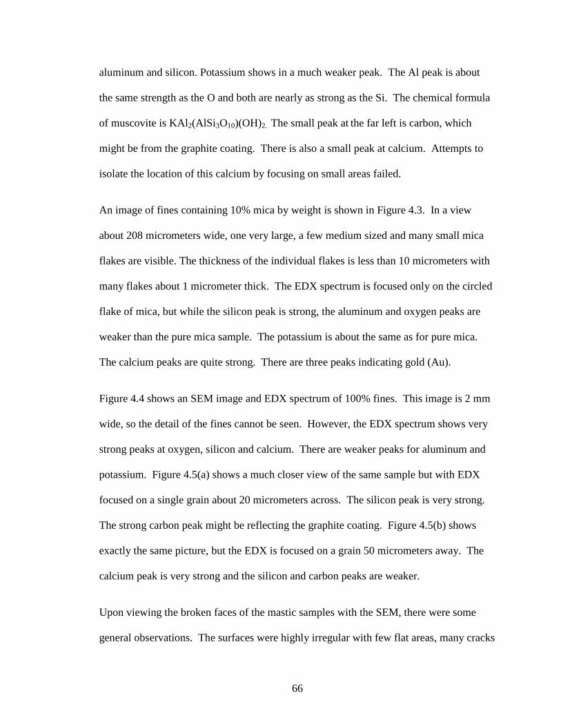
66
aluminum and silicon. Potassium shows in a much weaker peak. The Al peak is about
the same strength as the O and both are nearly as strong as the Si. The chemical formula
of muscovite is KAl2(AlSi3O10)(OH)2. The small peak at the far left is carbon, which
might be from the graphite coating. There is also a small peak at calcium. Attempts to
isolate the location of this calcium by focusing on small areas failed.
An image of fines containing 10% mica by weight is shown in Figure 4.3. In a view
about 208 micrometers wide, one very large, a few medium sized and many small mica
flakes are visible. The thickness of the individual flakes is less than 10 micrometers with
many flakes about 1 micrometer thick. The EDX spectrum is focused only on the circled
flake of mica, but while the silicon peak is strong, the aluminum and oxygen peaks are
weaker than the pure mica sample. The potassium is about the same as for pure mica.
The calcium peaks are quite strong. There are three peaks indicating gold (Au).
Figure 4.4 shows an SEM image and EDX spectrum of 100% fines. This image is 2 mm
wide, so the detail of the fines cannot be seen. However, the EDX spectrum shows very
strong peaks at oxygen, silicon and calcium. There are weaker peaks for aluminum and
potassium. Figure 4.5(a) shows a much closer view of the same sample but with EDX
focused on a single grain about 20 micrometers across. The silicon peak is very strong.
The strong carbon peak might be reflecting the graphite coating. Figure 4.5(b) shows
exactly the same picture, but the EDX is focused on a grain 50 micrometers away. The
calcium peak is very strong and the silicon and carbon peaks are weaker.
Upon viewing the broken faces of the mastic samples with the SEM, there were some
general observations. The surfaces were highly irregular with few flat areas, many cracks
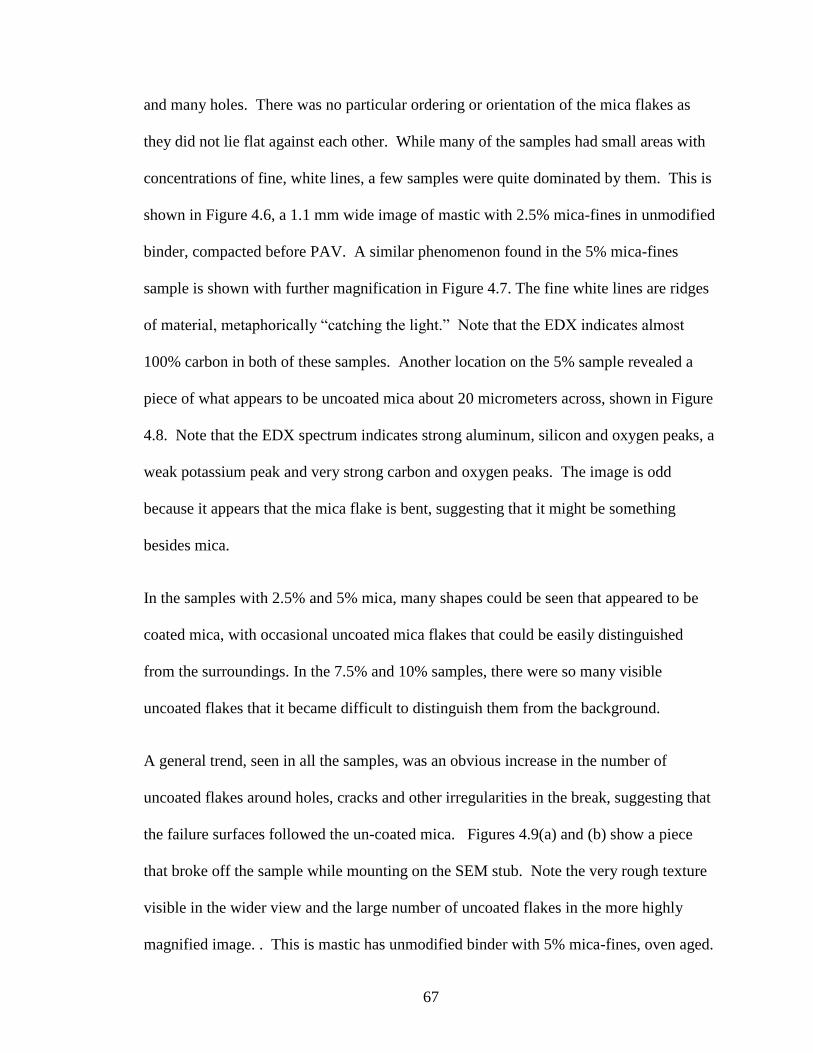
67
and many holes. There was no particular ordering or orientation of the mica flakes as
they did not lie flat against each other. While many of the samples had small areas with
concentrations of fine, white lines, a few samples were quite dominated by them. This is
shown in Figure 4.6, a 1.1 mm wide image of mastic with 2.5% mica-fines in unmodified
binder, compacted before PAV. A similar phenomenon found in the 5% mica-fines
sample is shown with further magnification in Figure 4.7. The fine white lines are ridges
of material, metaphorically “catching the light.” Note that the EDX indicates almost
100% carbon in both of these samples. Another location on the 5% sample revealed a
piece of what appears to be uncoated mica about 20 micrometers across, shown in Figure
4.8. Note that the EDX spectrum indicates strong aluminum, silicon and oxygen peaks, a
weak potassium peak and very strong carbon and oxygen peaks. The image is odd
because it appears that the mica flake is bent, suggesting that it might be something
besides mica.
In the samples with 2.5% and 5% mica, many shapes could be seen that appeared to be
coated mica, with occasional uncoated mica flakes that could be easily distinguished
from the surroundings. In the 7.5% and 10% samples, there were so many visible
uncoated flakes that it became difficult to distinguish them from the background.
A general trend, seen in all the samples, was an obvious increase in the number of
uncoated flakes around holes, cracks and other irregularities in the break, suggesting that
the failure surfaces followed the un-coated mica. Figures 4.9(a) and (b) show a piece
that broke off the sample while mounting on the SEM stub. Note the very rough texture
visible in the wider view and the large number of uncoated flakes in the more highly
magnified image. . This is mastic has unmodified binder with 5% mica-fines, oven aged.
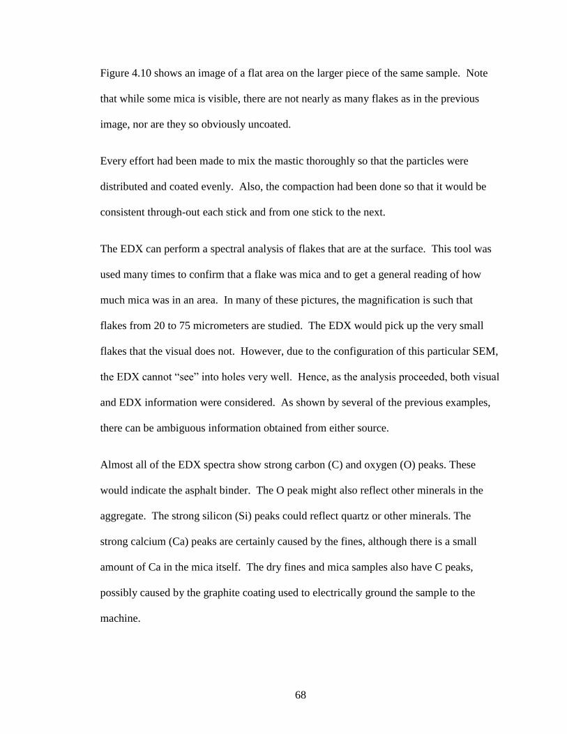
68
Figure 4.10 shows an image of a flat area on the larger piece of the same sample. Note
that while some mica is visible, there are not nearly as many flakes as in the previous
image, nor are they so obviously uncoated.
Every effort had been made to mix the mastic thoroughly so that the particles were
distributed and coated evenly. Also, the compaction had been done so that it would be
consistent through-out each stick and from one stick to the next.
The EDX can perform a spectral analysis of flakes that are at the surface. This tool was
used many times to confirm that a flake was mica and to get a general reading of how
much mica was in an area. In many of these pictures, the magnification is such that
flakes from 20 to 75 micrometers are studied. The EDX would pick up the very small
flakes that the visual does not. However, due to the configuration of this particular SEM,
the EDX cannot “see” into holes very well. Hence, as the analysis proceeded, both visual
and EDX information were considered. As shown by several of the previous examples,
there can be ambiguous information obtained from either source.
Almost all of the EDX spectra show strong carbon (C) and oxygen (O) peaks. These
would indicate the asphalt binder. The O peak might also reflect other minerals in the
aggregate. The strong silicon (Si) peaks could reflect quartz or other minerals. The
strong calcium (Ca) peaks are certainly caused by the fines, although there is a small
amount of Ca in the mica itself. The dry fines and mica samples also have C peaks,
possibly caused by the graphite coating used to electrically ground the sample to the
machine.
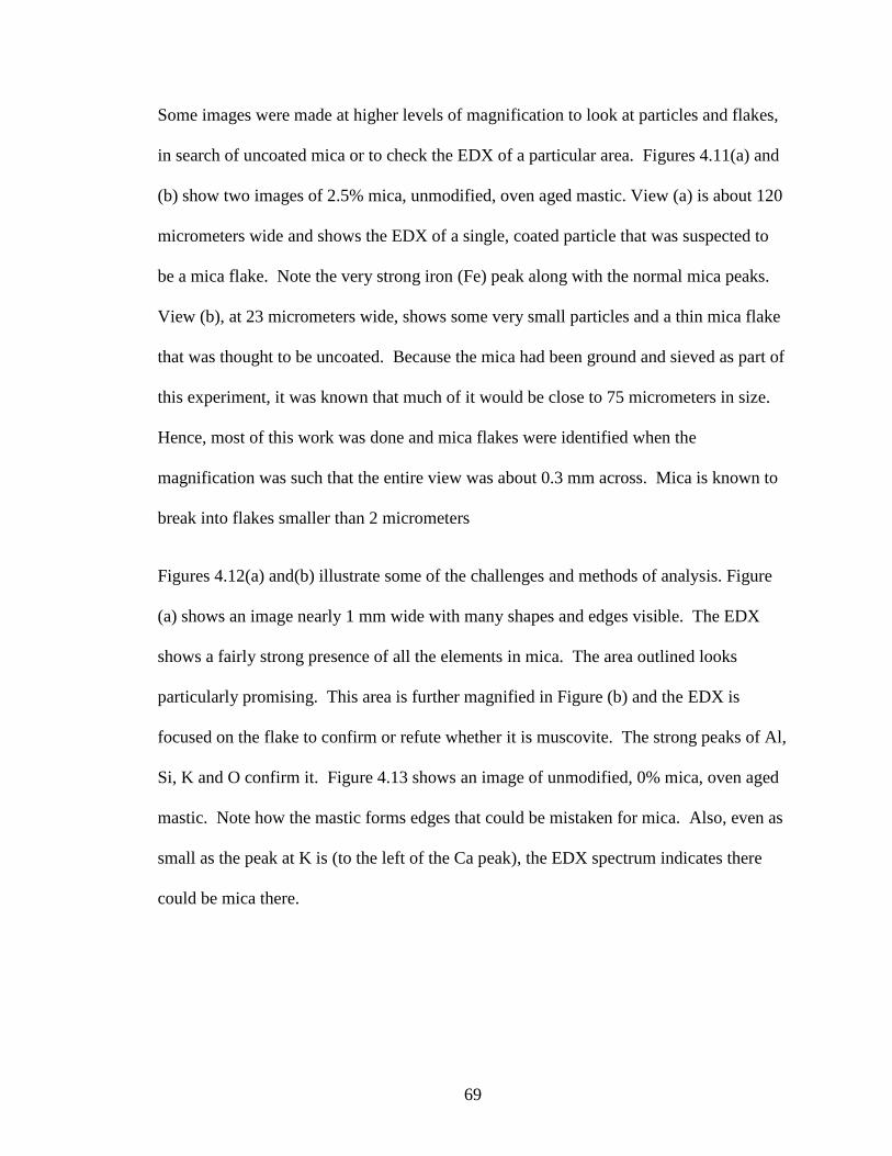
69
Some images were made at higher levels of magnification to look at particles and flakes,
in search of uncoated mica or to check the EDX of a particular area. Figures 4.11(a) and
(b) show two images of 2.5% mica, unmodified, oven aged mastic. View (a) is about 120
micrometers wide and shows the EDX of a single, coated particle that was suspected to
be a mica flake. Note the very strong iron (Fe) peak along with the normal mica peaks.
View (b), at 23 micrometers wide, shows some very small particles and a thin mica flake
that was thought to be uncoated. Because the mica had been ground and sieved as part of
this experiment, it was known that much of it would be close to 75 micrometers in size.
Hence, most of this work was done and mica flakes were identified when the
magnification was such that the entire view was about 0.3 mm across. Mica is known to
break into flakes smaller than 2 micrometers
Figures 4.12(a) and(b) illustrate some of the challenges and methods of analysis. Figure
(a) shows an image nearly 1 mm wide with many shapes and edges visible. The EDX
shows a fairly strong presence of all the elements in mica. The area outlined looks
particularly promising. This area is further magnified in Figure (b) and the EDX is
focused on the flake to confirm or refute whether it is muscovite. The strong peaks of Al,
Si, K and O confirm it. Figure 4.13 shows an image of unmodified, 0% mica, oven aged
mastic. Note how the mastic forms edges that could be mistaken for mica. Also, even as
small as the peak at K is (to the left of the Ca peak), the EDX spectrum indicates there
could be mica there.
70
4.3 Conclusion
Generally, mastics containing concentrations of mica greater than 5% were very dry,
difficult to handle and showed so many flakes in the SEM that were either uncoated or
only lightly coated that it was difficult to analyze. There were more uncoated flakes seen
in holes and cracks than on flat, stable areas. There was a small, inconsistent progression
of increase to the number of uncoated flakes seen as the aging increased from oven aged
to RTFO to Post-PAV. The samples molded Pre-PAV had a slightly higher increase.
Unaged samples showed very few uncoated flakes. While aging is not insignificant, mica
concentration seems to have a greater influence over the number of uncoated flakes than
aging does.
The literature suggests that the mica flakes would be lying flat against each other. Also,
while handling the larger pieces of mica during the cleaning and grinding processes, it
did seem that the flakes tended to lie flat against one another. However, in the mastics,
there was great disorder in the arrangement of the mica flakes and the broken surfaces
were irregular, with many cracks and holes rather than flat.
According to the literature, a large piece of muscovite showing a smooth, flat surface has
the EDX spectrum with following peaks: aluminum (Al) at 1.5 Kev, silicon (Si) at
1.75Kev and potassium (K) at 3.25 Kev in two peaks. There is no mention of oxygen.
EDX spectra in this experiment show the expected peaks at aluminum, silicon and
potassium. But there is also a strong peak at oxygen. The chemical formula of
muscovite, KAl2(AlSi3O10)(OH)2, indicates there is quite a bit of oxygen in the mineral.
71
One explanation for the difference in the EDX pattern might be that, in this experiment,
the mica was ground fine and all surfaces were visible to the EDX.
Generally, in images of mastic showing a view wider than .5 mm, the EDX carbon peak
is very strong compared to all other peaks. The calcium and silicon peaks compete for
second strongest, with calcium tending to be stronger in the lower mica-content samples
and silicon stronger in the higher mica-content samples. The oxygen peak is quite
variable, ranging from very short to as tall as the silicon. The height of the aluminum
peak increases with mica content, as does the potassium peak. In more highly magnified
images, the height of the carbon peak decreases as the number of mica flakes increases,
particularly when the EDX is focused on a concentration of flakes, suggesting that the
flakes are not coated with binder.
An earlier calculation in this study yielded surface areas for 1 cubic mm of material for a
sphere as being under 5 mm2. As the literature reports a thickness of 25 micrometers for
mica flakes, a calculation of the surface area of a disk of 1 cubic mm and 25 micrometers
thick yielded a surface area of 80 mm2. The SEM images clearly show the thickness of
mica at 1 micrometer and a similar calculation leads to the surface area of 1 cubic mm
being over 2000 mm2.
Table 4.1 shows an abbreviated listing of the counts of flakes seen on the fractured faces
of the unmodified samples of 2.5%, 5% and 75% mica mastics. Table 4.2 lists general
observations of the same samples. Table 4.3 and Table 4.4 list the same information for
the SB4% modified samples. Appendix A contains detailed descriptions of all the
observations made on the SEM and comparisons between samples..
72
(a): Sample on SEM stub
(b): SEM image of mica in AC
(c): SEM image of AC showing cracked mica
Figure 4.1: Original AC sample
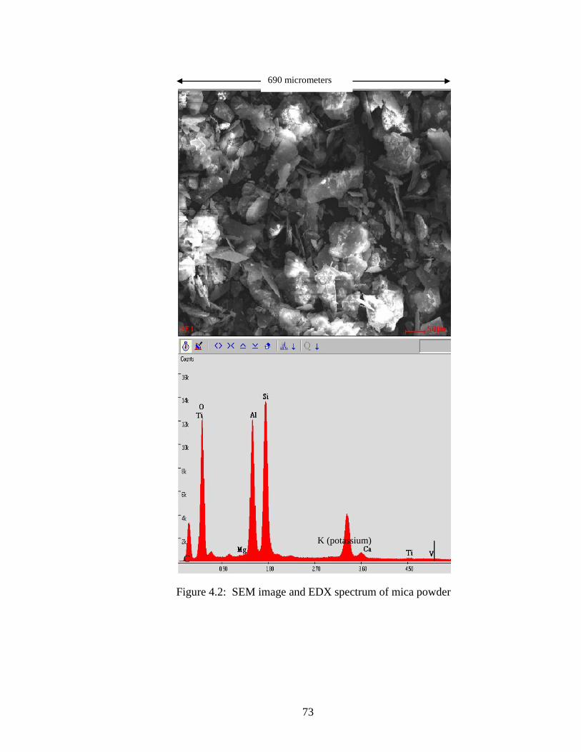
73
Figure 4.2: SEM image and EDX spectrum of mica powder
K (potassium)
C
690 micrometers
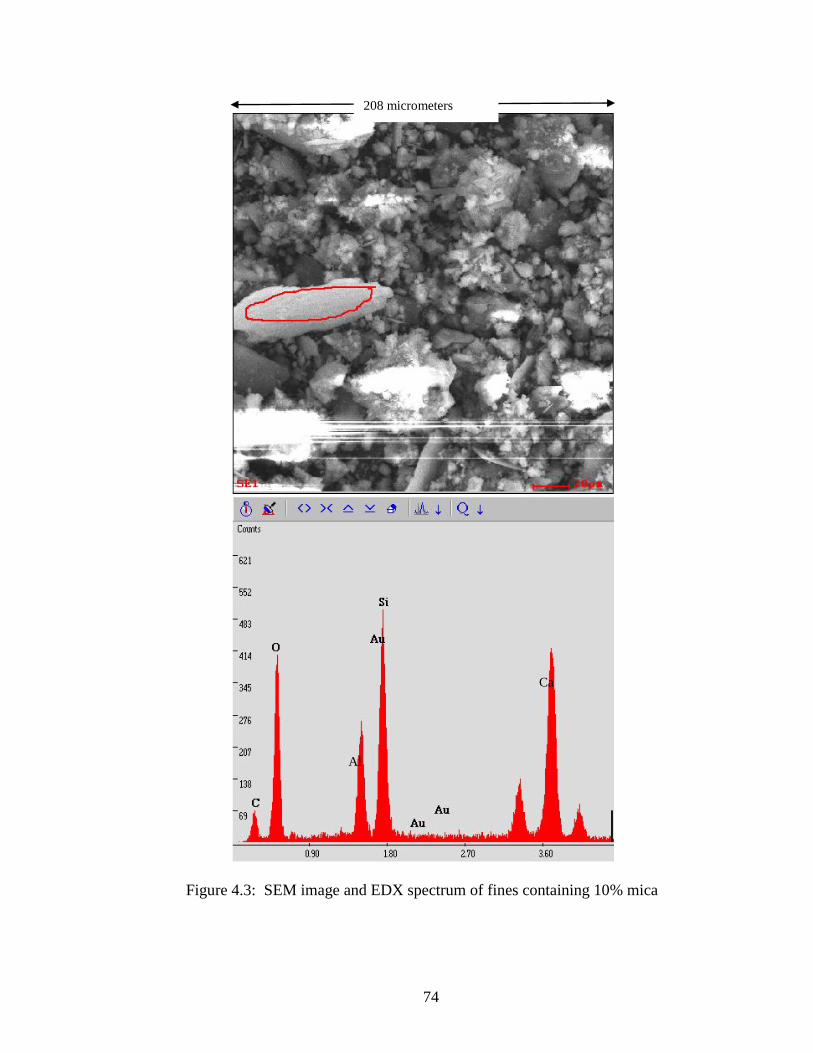
74
Figure 4.3: SEM image and EDX spectrum of fines containing 10% mica
Ca
Al
208 micrometers
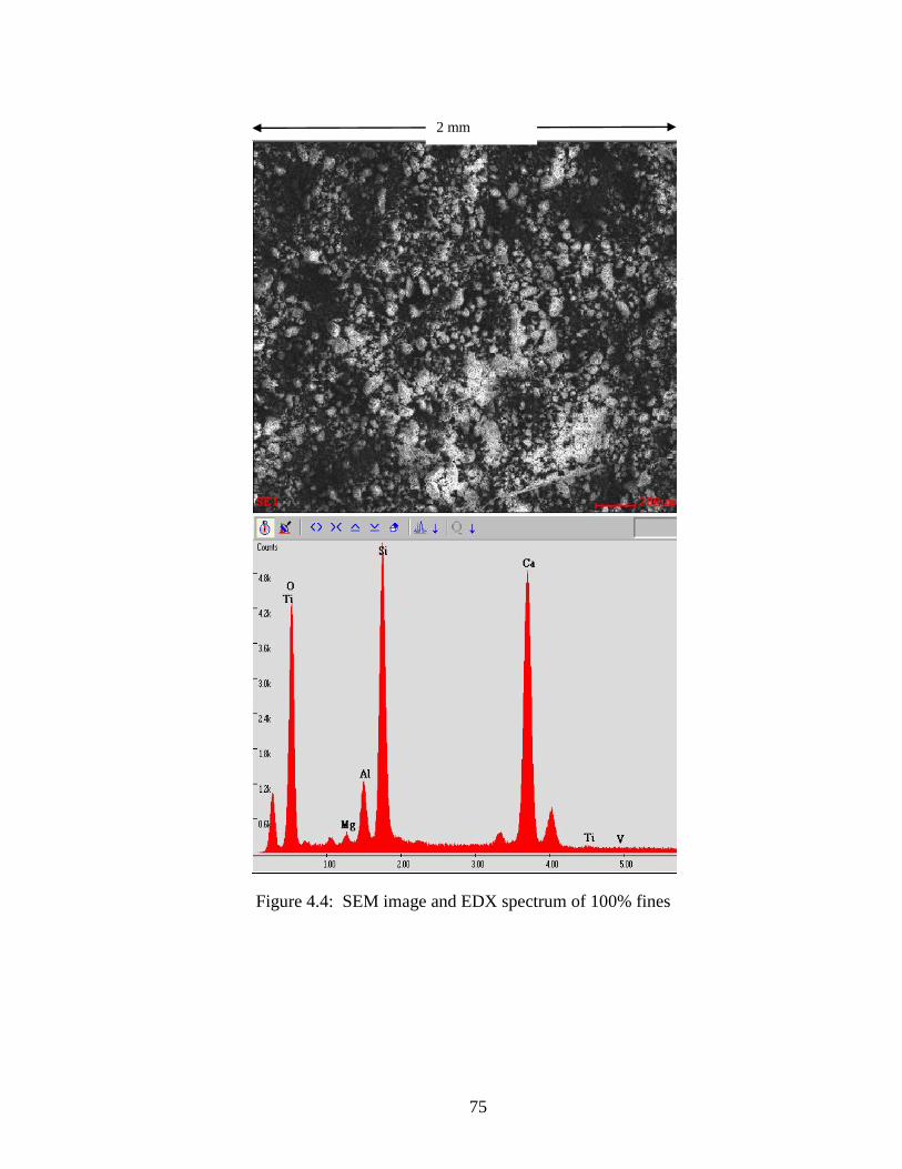
75
Figure 4.4: SEM image and EDX spectrum of 100% fines
2 mm
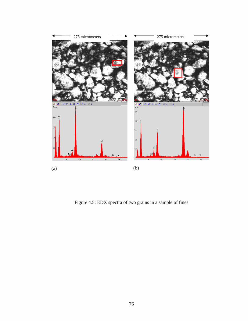
76
(b)
(a)
275 micrometers 275 micrometers
Figure 4.5: EDX spectra of two grains in a sample of fines
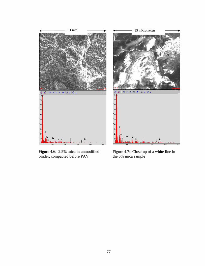
77
Figure 4.7: Close-up of a white line in
the 5% mica sample
Figure 4.6: 2.5% mica in unmodified
binder, compacted before PAV
1.1 mm 85 micrometers
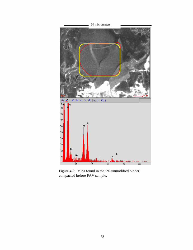
78
Figure 4.8: Mica found in the 5% unmodified binder,
compacted before PAV sample.
50 micrometers
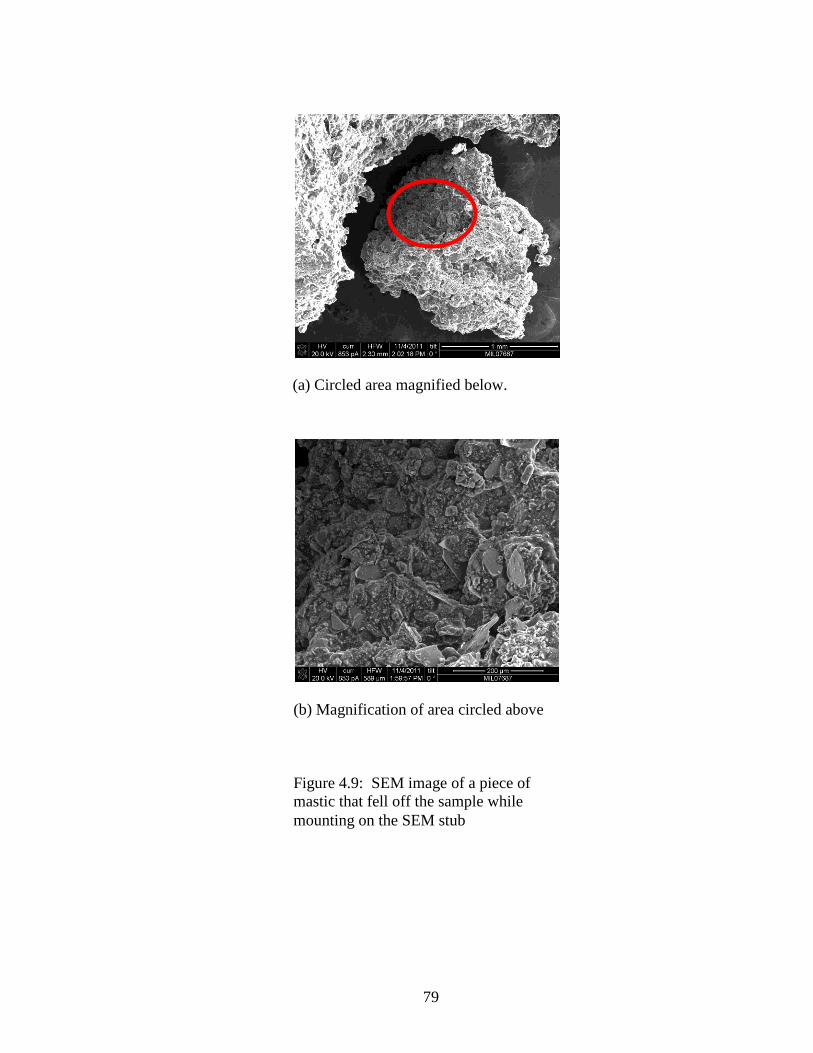
79
(a) Circled area magnified below.
(b) Magnification of area circled above
Figure 4.9: SEM image of a piece of
mastic that fell off the sample while
mounting on the SEM stub
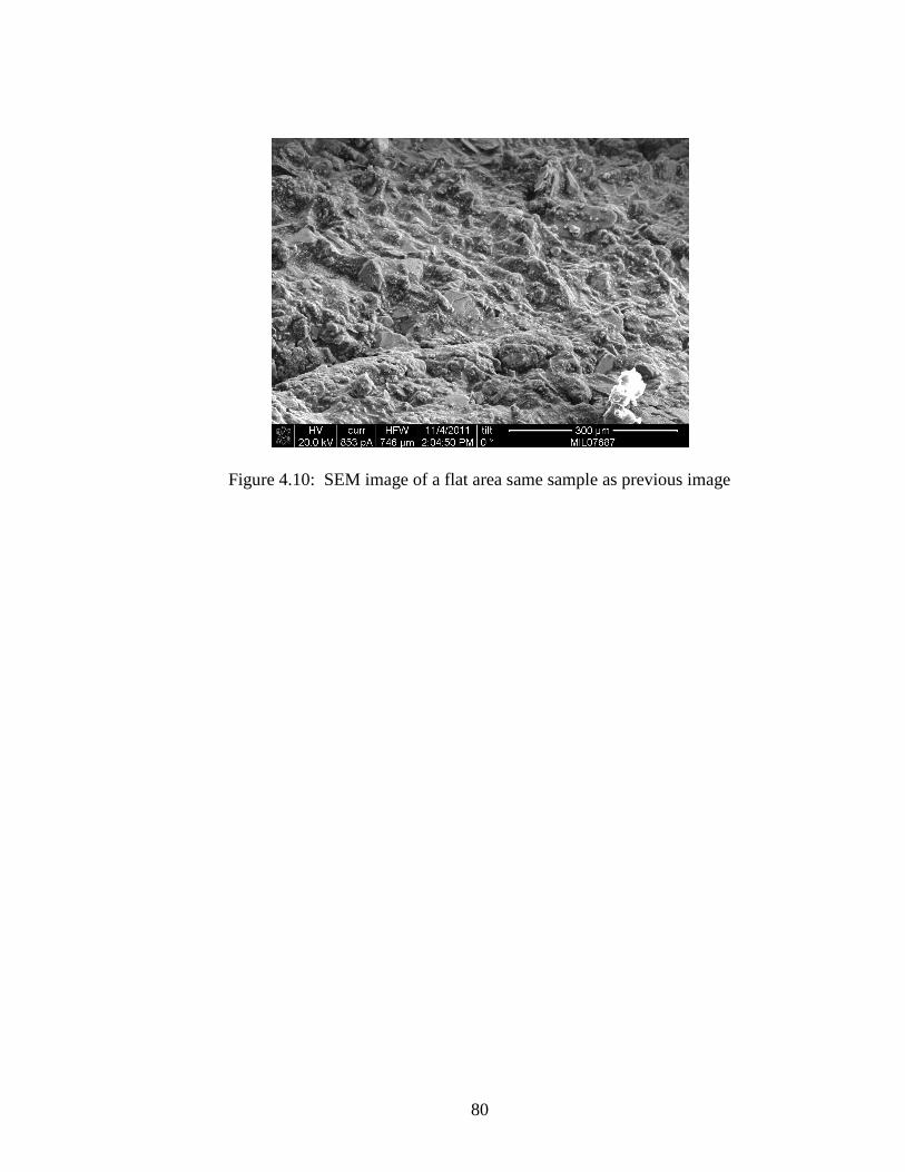
80
Figure 4.10: SEM image of a flat area same sample as previous image
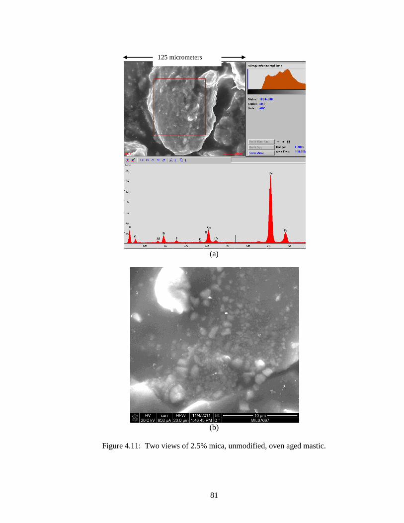
81
(a)
(b)
Figure 4.11: Two views of 2.5% mica, unmodified, oven aged mastic.
125 micrometers
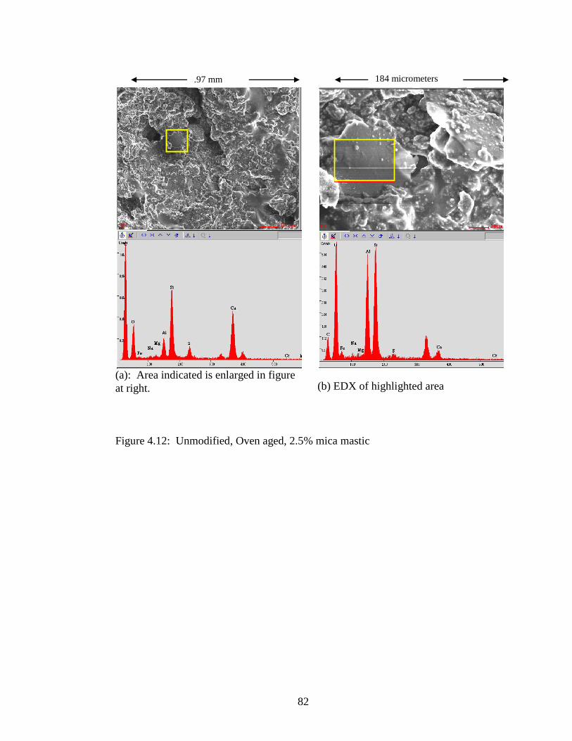
82
(a): Area indicated is enlarged in figure
at right.
(b) EDX of highlighted area
Figure 4.12: Unmodified, Oven aged, 2.5% mica mastic
.97 mm 184 micrometers
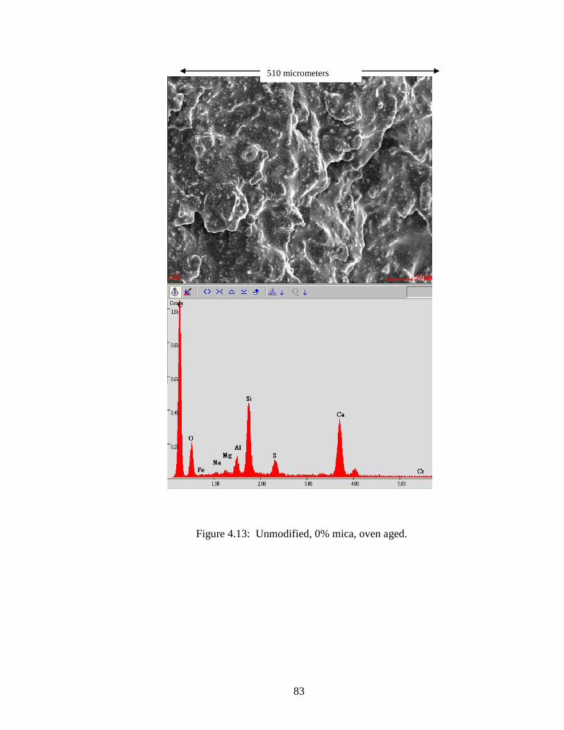
83
Figure 4.13: Unmodified, 0% mica, oven aged.
510 micrometers
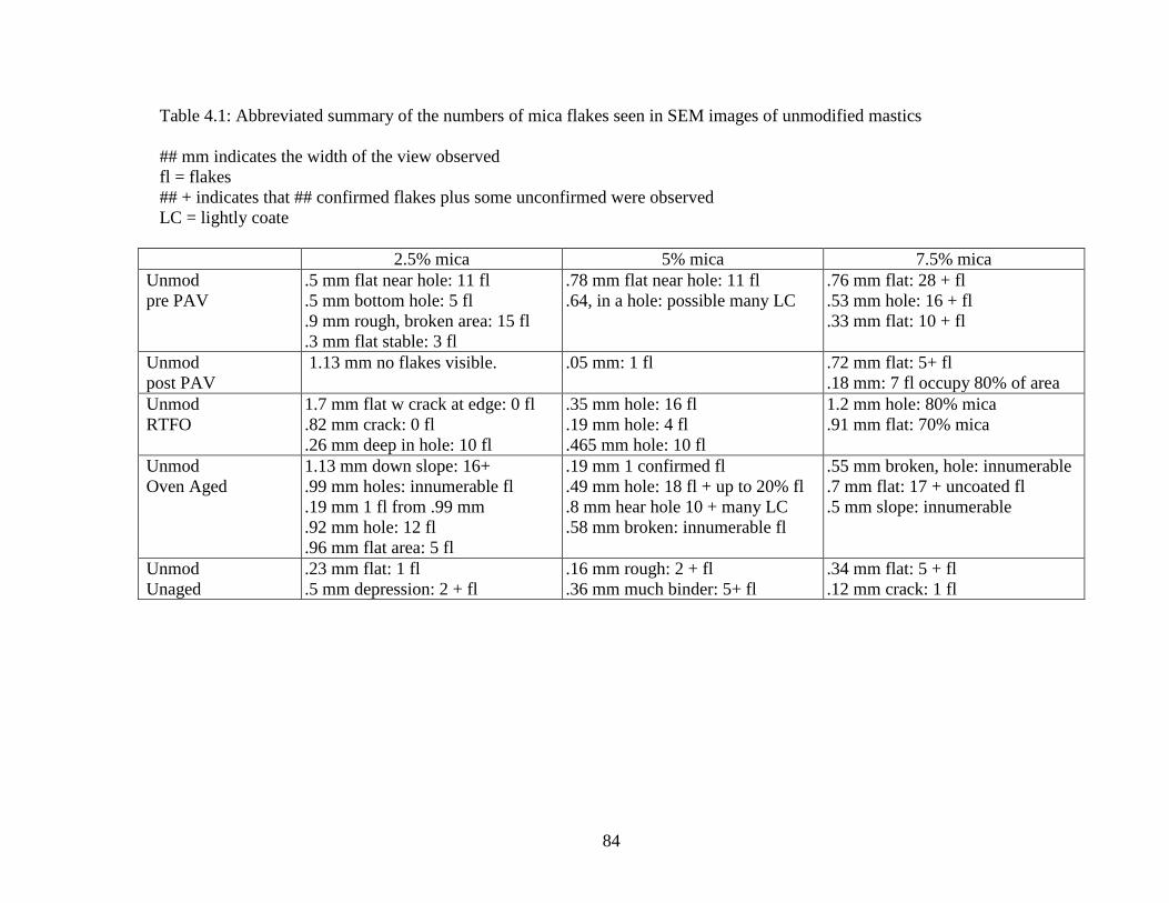
84
Table 4.1: Abbreviated summary of the numbers of mica flakes seen in SEM images of unmodified mastics
## mm indicates the width of the view observed
fl = flakes
## + indicates that ## confirmed flakes plus some unconfirmed were observed
LC = lightly coate
2.5% mica 5% mica 7.5% mica
Unmod
pre PAV
.5 mm flat near hole: 11 fl
.5 mm bottom hole: 5 fl
.9 mm rough, broken area: 15 fl
.3 mm flat stable: 3 fl
.78 mm flat near hole: 11 fl
.64, in a hole: possible many LC
.76 mm flat: 28 + fl
.53 mm hole: 16 + fl
.33 mm flat: 10 + fl
Unmod
post PAV
1.13 mm no flakes visible. .05 mm: 1 fl
.72 mm flat: 5+ fl
.18 mm: 7 fl occupy 80% of area
Unmod
RTFO
1.7 mm flat w crack at edge: 0 fl
.82 mm crack: 0 fl
.26 mm deep in hole: 10 fl
.35 mm hole: 16 fl
.19 mm hole: 4 fl
.465 mm hole: 10 fl
1.2 mm hole: 80% mica
.91 mm flat: 70% mica
Unmod
Oven Aged
1.13 mm down slope: 16+
.99 mm holes: innumerable fl
.19 mm 1 fl from .99 mm
.92 mm hole: 12 fl
.96 mm flat area: 5 fl
.19 mm 1 confirmed fl
.49 mm hole: 18 fl + up to 20% fl
.8 mm hear hole 10 + many LC
.58 mm broken: innumerable fl
.55 mm broken, hole: innumerable
.7 mm flat: 17 + uncoated fl
.5 mm slope: innumerable
Unmod
Unaged
.23 mm flat: 1 fl
.5 mm depression: 2 + fl
.16 mm rough: 2 + fl
.36 mm much binder: 5+ fl
.34 mm flat: 5 + fl
.12 mm crack: 1 fl
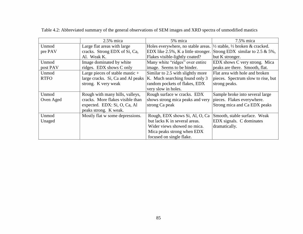
85
Table 4.2: Abbreviated summary of the general observations of SEM images and XRD spectra of unmodified mastics
2.5% mica 5% mica 7.5% mica
Unmod
pre PAV
Large flat areas with large
cracks. Strong EDX of Si, Ca,
Al. Weak K.
Holes everywhere, no stable areas.
EDX like 2.5%, K a little stronger.
Flakes visible-lightly coated?
½ stable, ½ broken & cracked.
Strong EDX similar to 2.5 & 5%,
but K stronger.
Unmod
post PAV
Image dominated by white
ridges. EDX shows C only
Many white “ridges” over entire
image. Seems to be binder.
EDX shows C very strong. Mica
peaks are there. Smooth, flat.
Unmod
RTFO
Large pieces of stable mastic +
large cracks. Si, Ca and Al peaks
strong. K very weak
Similar to 2.5 with slightly more
K. Much searching found only 3
random pockets of flakes, EDX
very slow in holes.
Flat area with hole and broken
pieces. Spectrum slow to rise, but
strong peaks.
Unmod
Oven Aged
Rough with many hills, valleys,
cracks. More flakes visible than
expected. EDX: Si, O, Ca, Al
peaks strong. K weak.
Rough surface w cracks. EDX
shows strong mica peaks and very
strong Ca peak
Sample broke into several large
pieces. Flakes everywhere.
Strong mica and Ca EDX peaks
Unmod
Unaged
Mostly flat w some depressions. Rough, EDX shows Si, Al, O, Ca
but lacks K in several areas.
Wider views showed no mica.
Mica peaks strong when EDX
focused on single flake.
Smooth, stable surface. Weak
EDX signals. C dominates
dramatically.
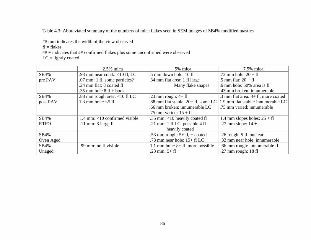
86
Table 4.3: Abbreviated summary of the numbers of mica flakes seen in SEM images of SB4% modified mastics
## mm indicates the width of the view observed
fl = flakes
## + indicates that ## confirmed flakes plus some unconfirmed were observed
LC = lightly coated
2.5% mica 5% mica 7.5% mica
SB4%
pre PAV
.93 mm near crack: <10 fl, LC
.07 mm: 1 fl, some particles?
.24 mm flat: 8 coated fl
.35 mm hole 8 fl + book
.5 mm down hole: 10 fl
.34 mm flat area: 1 fl large
Many flake shapes
.72 mm hole: 20 + fl
.5 mm flat: 20 + fl
.6 mm hole: 50% area is fl
.43 mm broken: innumerable
SB4%
post PAV
.88 mm rough area: <10 fl LC
1.3 mm hole: <5 fl
.23 mm rough: 4+ fl
.88 mm flat stable: 20+ fl, some LC
.66 mm broken: innumerable LC
.75 mm varied: 15 + fl
.3 mm flat area: 3+ fl, more coated
1.9 mm flat stable: innumerable LC
.75 mm varied: innumerable
SB4%
RTFO
1.4 mm: <10 confirmed visible
.11 mm: 3 large fl
.35 mm: <10 heavily coated fl
.21 mm: 1 fl LC possible 4 fl
heavily coated
1.4 mm slopes holes: 25 + fl
.27 mm slope: 14 +
SB4%
Oven Aged
.53 mm rough: 5+ fl, + coated
.73 mm near hole: 15+ fl LC
.26 rough: 5 fl unclear
.32 mm near hole: innumerable
SB4%
Unaged
.99 mm: no fl visible 1.1 mm hole: 8+ fl more possible
.23 mm: 5+ fl
.66 mm rough: innumerable fl
.27 mm rough: 18 fl
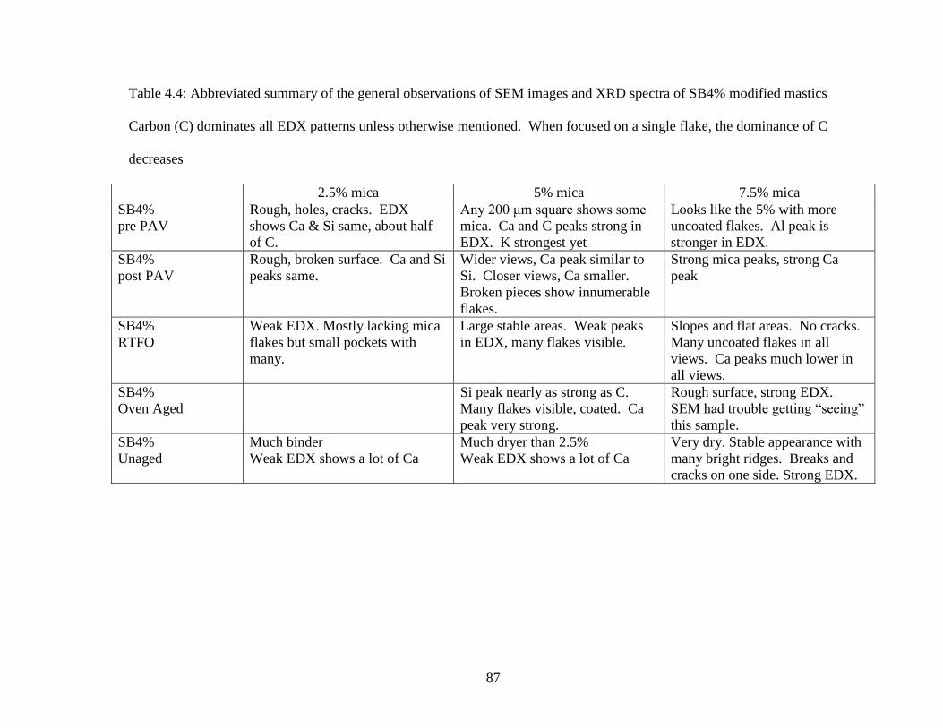
87
Table 4.4: Abbreviated summary of the general observations of SEM images and XRD spectra of SB4% modified mastics
Carbon (C) dominates all EDX patterns unless otherwise mentioned. When focused on a single flake, the dominance of C
decreases
2.5% mica 5% mica 7.5% mica
SB4%
pre PAV
Rough, holes, cracks. EDX
shows Ca & Si same, about half
of C.
Any 200 μm square shows some
mica. Ca and C peaks strong in
EDX. K strongest yet
Looks like the 5% with more
uncoated flakes. Al peak is
stronger in EDX.
SB4%
post PAV
Rough, broken surface. Ca and Si
peaks same.
Wider views, Ca peak similar to
Si. Closer views, Ca smaller.
Broken pieces show innumerable
flakes.
Strong mica peaks, strong Ca
peak
SB4%
RTFO
Weak EDX. Mostly lacking mica
flakes but small pockets with
many.
Large stable areas. Weak peaks
in EDX, many flakes visible.
Slopes and flat areas. No cracks.
Many uncoated flakes in all
views. Ca peaks much lower in
all views.
SB4%
Oven Aged
Si peak nearly as strong as C.
Many flakes visible, coated. Ca
peak very strong.
Rough surface, strong EDX.
SEM had trouble getting “seeing”
this sample.
SB4%
Unaged
Much binder
Weak EDX shows a lot of Ca
Much dryer than 2.5%
Weak EDX shows a lot of Ca
Very dry. Stable appearance with
many bright ridges. Breaks and
cracks on one side. Strong EDX.
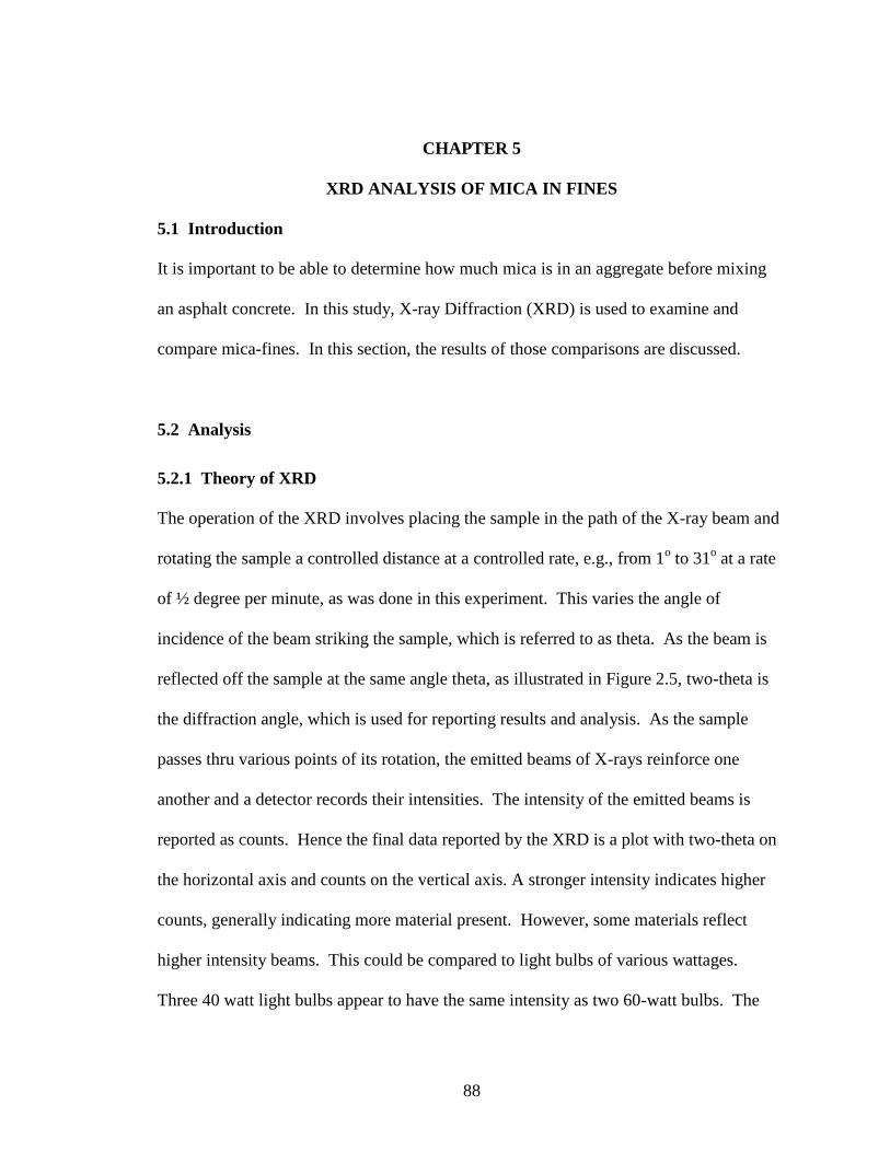
88
CHAPTER 5
XRD ANALYSIS OF MICA IN FINES
5.1 Introduction
It is important to be able to determine how much mica is in an aggregate before mixing
an asphalt concrete. In this study, X-ray Diffraction (XRD) is used to examine and
compare mica-fines. In this section, the results of those comparisons are discussed.
5.2 Analysis
5.2.1 Theory of XRD
The operation of the XRD involves placing the sample in the path of the X-ray beam and
rotating the sample a controlled distance at a controlled rate, e.g., from 1o to 31
o at a rate
of ½ degree per minute, as was done in this experiment. This varies the angle of
incidence of the beam striking the sample, which is referred to as theta. As the beam is
reflected off the sample at the same angle theta, as illustrated in Figure 2.5, two-theta is
the diffraction angle, which is used for reporting results and analysis. As the sample
passes thru various points of its rotation, the emitted beams of X-rays reinforce one
another and a detector records their intensities. The intensity of the emitted beams is
reported as counts. Hence the final data reported by the XRD is a plot with two-theta on
the horizontal axis and counts on the vertical axis. A stronger intensity indicates higher
counts, generally indicating more material present. However, some materials reflect
higher intensity beams. This could be compared to light bulbs of various wattages.
Three 40 watt light bulbs appear to have the same intensity as two 60-watt bulbs. The
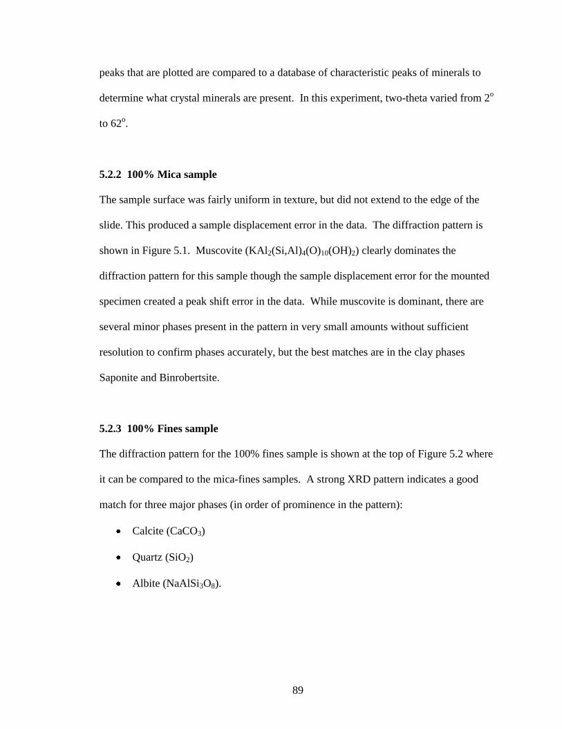
89
peaks that are plotted are compared to a database of characteristic peaks of minerals to
determine what crystal minerals are present. In this experiment, two-theta varied from 2o
to 62o.
5.2.2 100% Mica sample
The sample surface was fairly uniform in texture, but did not extend to the edge of the
slide. This produced a sample displacement error in the data. The diffraction pattern is
shown in Figure 5.1. Muscovite (KAl2(Si,Al)4(O)10(OH)2) clearly dominates the
diffraction pattern for this sample though the sample displacement error for the mounted
specimen created a peak shift error in the data. While muscovite is dominant, there are
several minor phases present in the pattern in very small amounts without sufficient
resolution to confirm phases accurately, but the best matches are in the clay phases
Saponite and Binrobertsite.
5.2.3 100% Fines sample
The diffraction pattern for the 100% fines sample is shown at the top of Figure 5.2 where
it can be compared to the mica-fines samples. A strong XRD pattern indicates a good
match for three major phases (in order of prominence in the pattern):
Calcite (CaCO3)
Quartz (SiO2)
Albite (NaAlSi3O8).
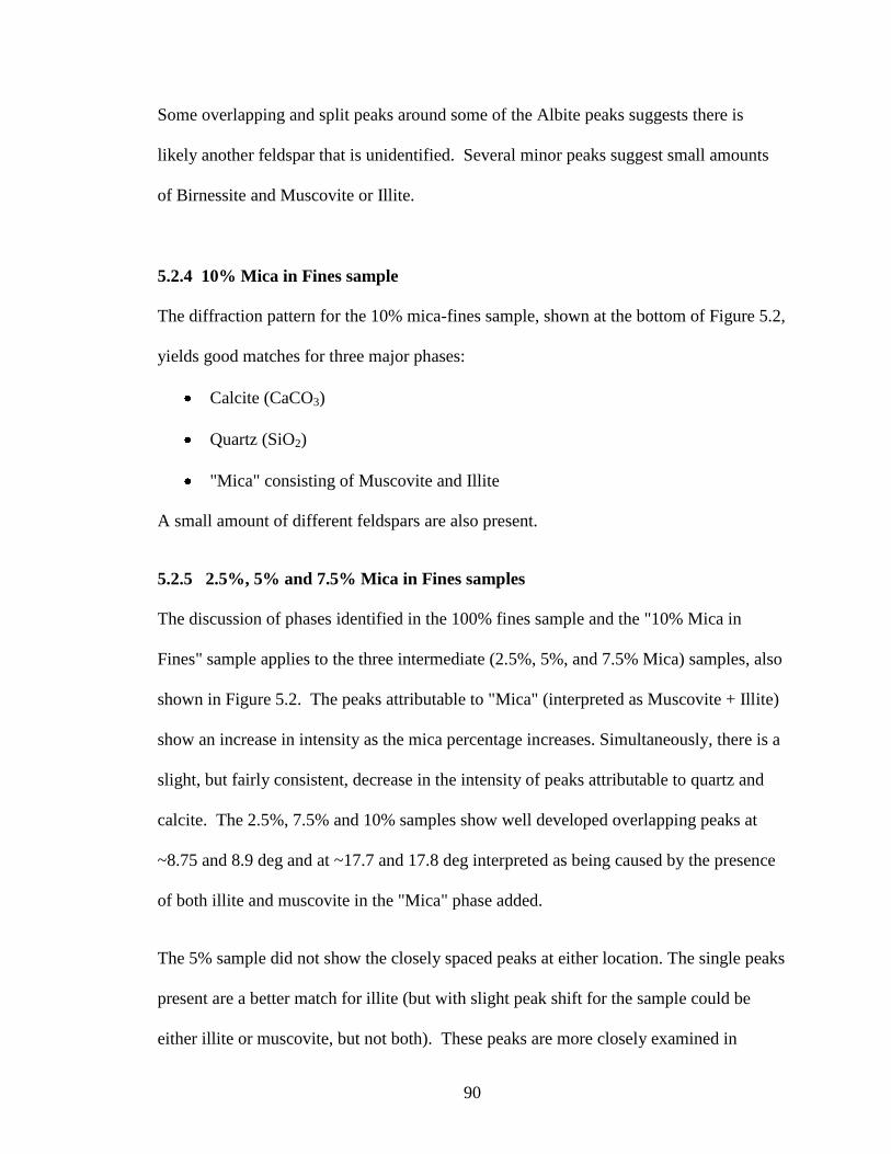
90
Some overlapping and split peaks around some of the Albite peaks suggests there is
likely another feldspar that is unidentified. Several minor peaks suggest small amounts
of Birnessite and Muscovite or Illite.
5.2.4 10% Mica in Fines sample
The diffraction pattern for the 10% mica-fines sample, shown at the bottom of Figure 5.2,
yields good matches for three major phases:
Calcite (CaCO3)
Quartz (SiO2)
"Mica" consisting of Muscovite and Illite
A small amount of different feldspars are also present.
5.2.5 2.5%, 5% and 7.5% Mica in Fines samples
The discussion of phases identified in the 100% fines sample and the "10% Mica in
Fines" sample applies to the three intermediate (2.5%, 5%, and 7.5% Mica) samples, also
shown in Figure 5.2. The peaks attributable to "Mica" (interpreted as Muscovite + Illite)
show an increase in intensity as the mica percentage increases. Simultaneously, there is a
slight, but fairly consistent, decrease in the intensity of peaks attributable to quartz and
calcite. The 2.5%, 7.5% and 10% samples show well developed overlapping peaks at
~8.75 and 8.9 deg and at ~17.7 and 17.8 deg interpreted as being caused by the presence
of both illite and muscovite in the "Mica" phase added.
The 5% sample did not show the closely spaced peaks at either location. The single peaks
present are a better match for illite (but with slight peak shift for the sample could be
either illite or muscovite, but not both). These peaks are more closely examined in
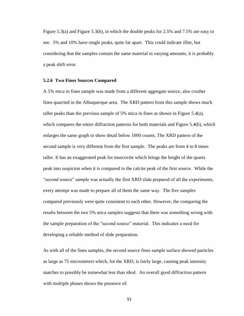
91
Figure 5.3(a) and Figure 5.3(b), in which the double peaks for 2.5% and 7.5% are easy to
see. 5% and 10% have single peaks, quite far apart. This could indicate illite, but
considering that the samples contain the same material in varying amounts, it is probably
a peak shift error.
5.2.6 Two Fines Sources Compared
A 5% mica in fines sample was made from a different aggregate source, also crusher
fines quarried in the Albuquerque area. The XRD pattern from this sample shows much
taller peaks than the previous sample of 5% mica in fines as shown in Figure 5.4(a),
which compares the entire diffraction patterns for both materials and Figure 5.4(b), which
enlarges the same graph to show detail below 1000 counts. The XRD pattern of the
second sample is very different from the first sample. The peaks are from 4 to 8 times
taller. It has an exaggerated peak for muscovite which brings the height of the quartz
peak into suspicion when it is compared to the calcite peak of the first source. While the
“second source” sample was actually the first XRD slide prepared of all the experiments,
every attempt was made to prepare all of them the same way. The five samples
compared previously were quite consistent to each other. However, the comparing the
results between the two 5% mica samples suggests that there was something wrong with
the sample preparation of the “second source” material. This indicates a need for
developing a reliable method of slide preparation.
As with all of the fines samples, the second source fines sample surface showed particles
as large as 75 micrometers which, for the XRD, is fairly large, causing peak intensity
matches to possibly be somewhat less than ideal. An overall good diffraction pattern
with multiple phases shows the presence of:
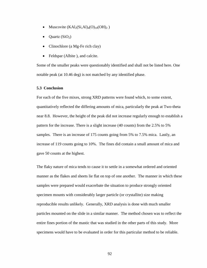
92
Muscovite (KAl2(Si,Al)4(O)10(OH)2 )
Quartz (SiO2)
Clinochlore (a Mg-Fe rich clay)
Feldspar (Albite ), and calcite.
Some of the smaller peaks were questionably identified and shall not be listed here. One
notable peak (at 10.46 deg) is not matched by any identified phase.
5.3 Conclusion
For each of the five mixes, strong XRD patterns were found which, to some extent,
quantitatively reflected the differing amounts of mica, particularly the peak at Two-theta
near 8.8. However, the height of the peak did not increase regularly enough to establish a
pattern for the increase. There is a slight increase (40 counts) from the 2.5% to 5%
samples. There is an increase of 175 counts going from 5% to 7.5% mica. Lastly, an
increase of 119 counts going to 10%. The fines did contain a small amount of mica and
gave 50 counts at the highest.
The flaky nature of mica tends to cause it to settle in a somewhat ordered and oriented
manner as the flakes and sheets lie flat on top of one another. The manner in which these
samples were prepared would exacerbate the situation to produce strongly oriented
specimen mounts with considerably larger particle (or crystallite) size making
reproducible results unlikely. Generally, XRD analysis is done with much smaller
particles mounted on the slide in a similar manner. The method chosen was to reflect the
entire fines portion of the mastic that was studied in the other parts of this study. More
specimens would have to be evaluated in order for this particular method to be reliable.

93
In summary,
XRD can be used to identify mica in an aggregate
XRD can, to an extent, be used to quantify mica in an aggregate
Proper sample preparation is critical
Similarities between the diffraction patterns of mica and illite can cause mis-
readings
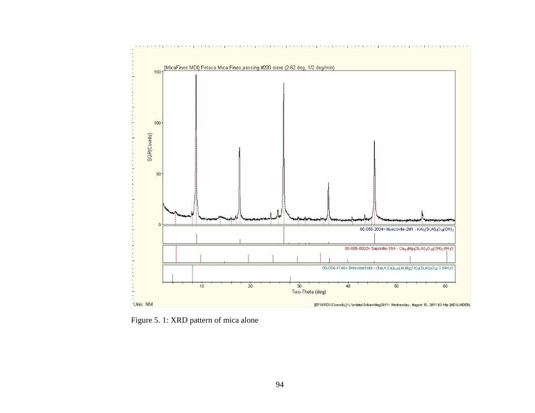
94
Figure 5. 1: XRD pattern of mica alone
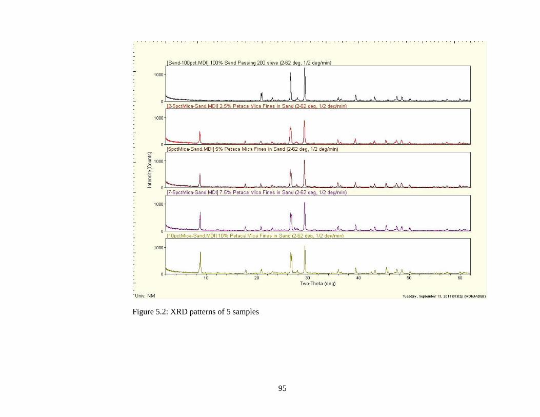
95
Figure 5.2: XRD patterns of 5 samples
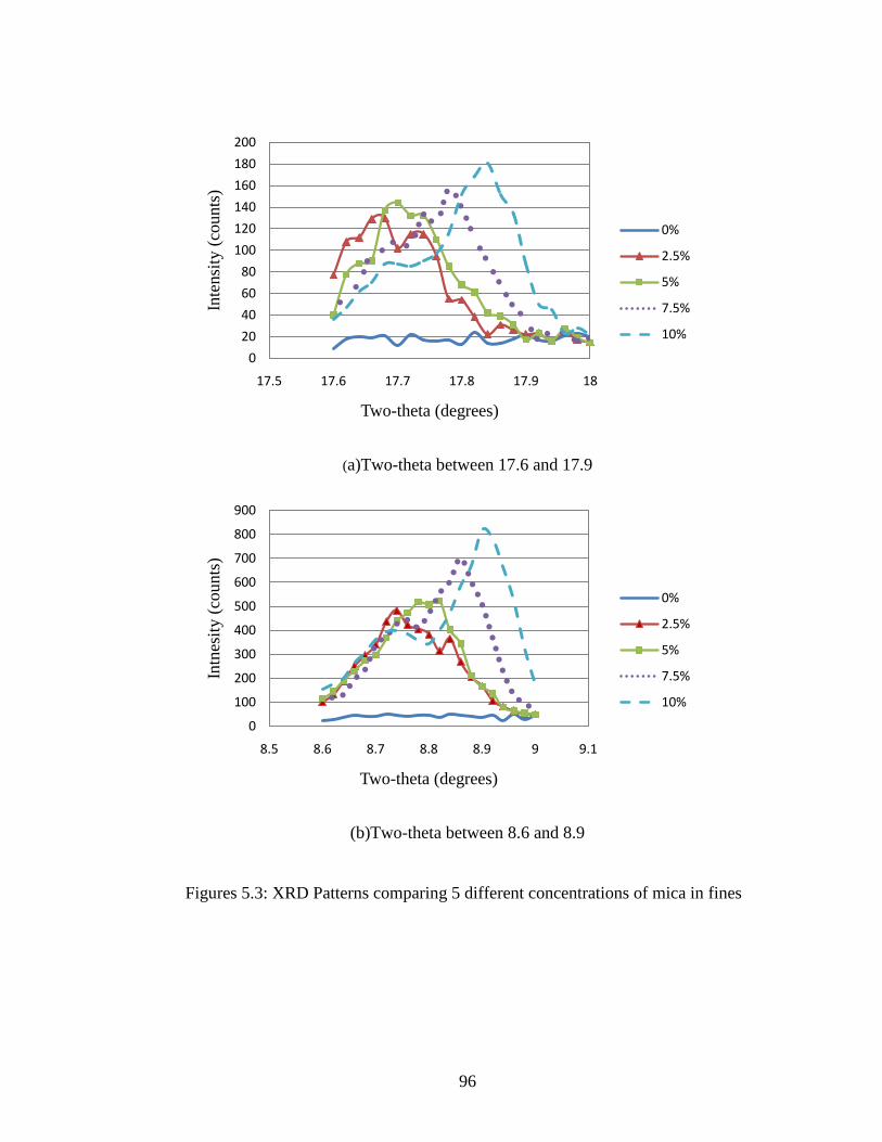
96
(a)Two-theta between 17.6 and 17.9
(b)Two-theta between 8.6 and 8.9
Figures 5.3: XRD Patterns comparing 5 different concentrations of mica in fines
0
20
40
60
80
100
120
140
160
180
200
17.5 17.6 17.7 17.8 17.9 18
Inte
nsi
ty (
counts
)
Two-theta (degrees)
0%
2.5%
5%
7.5%
10%
0
100
200
300
400
500
600
700
800
900
8.5 8.6 8.7 8.8 8.9 9 9.1
Intn
esit
y (
counts
)
Two-theta (degrees)
0%
2.5%
5%
7.5%
10%
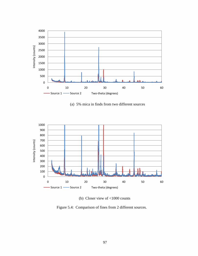
97
(a) 5% mica in finds from two different sources
(b) Closer view of <1000 counts
Figure 5.4: Comparison of fines from 2 different sources.
0
500
1000
1500
2000
2500
3000
3500
4000
0 10 20 30 40 50 60
Inte
nsi
ty (
cou
nts
)
Two-theta (degrees)Source 1 Source 2
0
100
200
300
400
500
600
700
800
900
1000
0 10 20 30 40 50 60
Inte
nsi
ty (
cou
nts
)
Two-theta (degrees)Source 1 Source 2
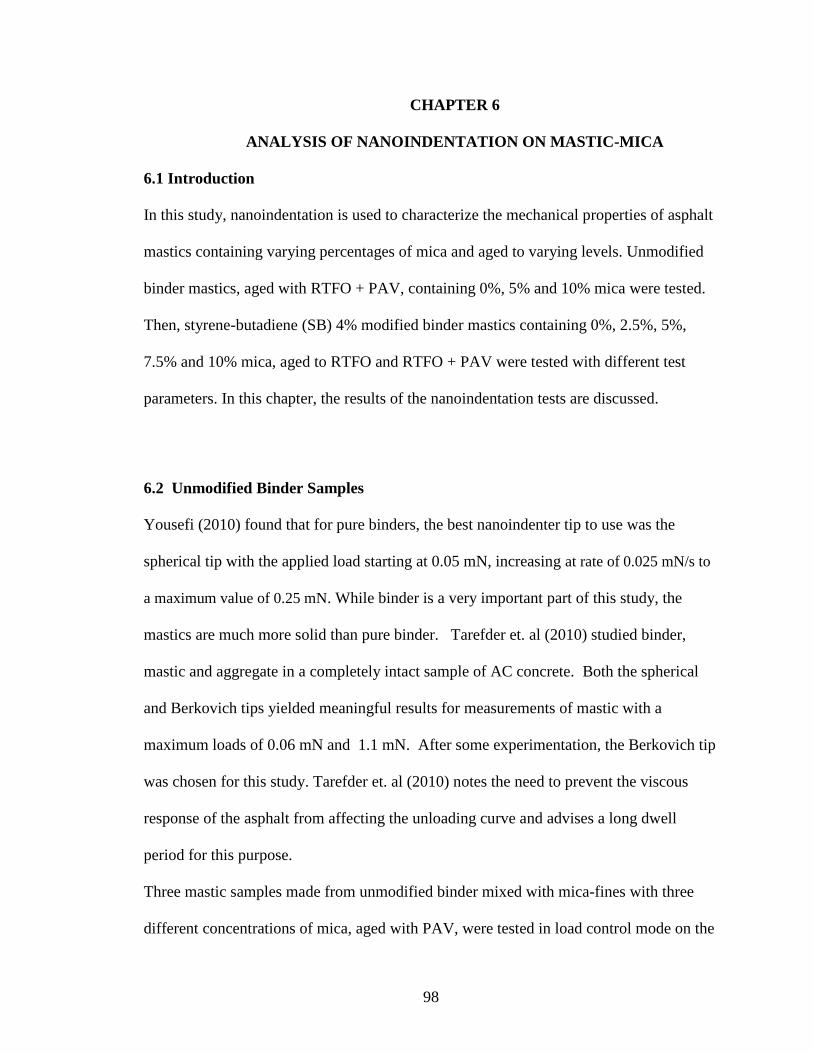
98
CHAPTER 6
ANALYSIS OF NANOINDENTATION ON MASTIC-MICA
6.1 Introduction
In this study, nanoindentation is used to characterize the mechanical properties of asphalt
mastics containing varying percentages of mica and aged to varying levels. Unmodified
binder mastics, aged with RTFO + PAV, containing 0%, 5% and 10% mica were tested.
Then, styrene-butadiene (SB) 4% modified binder mastics containing 0%, 2.5%, 5%,
7.5% and 10% mica, aged to RTFO and RTFO + PAV were tested with different test
parameters. In this chapter, the results of the nanoindentation tests are discussed.
6.2 Unmodified Binder Samples
Yousefi (2010) found that for pure binders, the best nanoindenter tip to use was the
spherical tip with the applied load starting at 0.05 mN, increasing at rate of 0.025 mN/s to
a maximum value of 0.25 mN. While binder is a very important part of this study, the
mastics are much more solid than pure binder. Tarefder et. al (2010) studied binder,
mastic and aggregate in a completely intact sample of AC concrete. Both the spherical
and Berkovich tips yielded meaningful results for measurements of mastic with a
maximum loads of 0.06 mN and 1.1 mN. After some experimentation, the Berkovich tip
was chosen for this study. Tarefder et. al (2010) notes the need to prevent the viscous
response of the asphalt from affecting the unloading curve and advises a long dwell
period for this purpose.
Three mastic samples made from unmodified binder mixed with mica-fines with three
different concentrations of mica, aged with PAV, were tested in load control mode on the
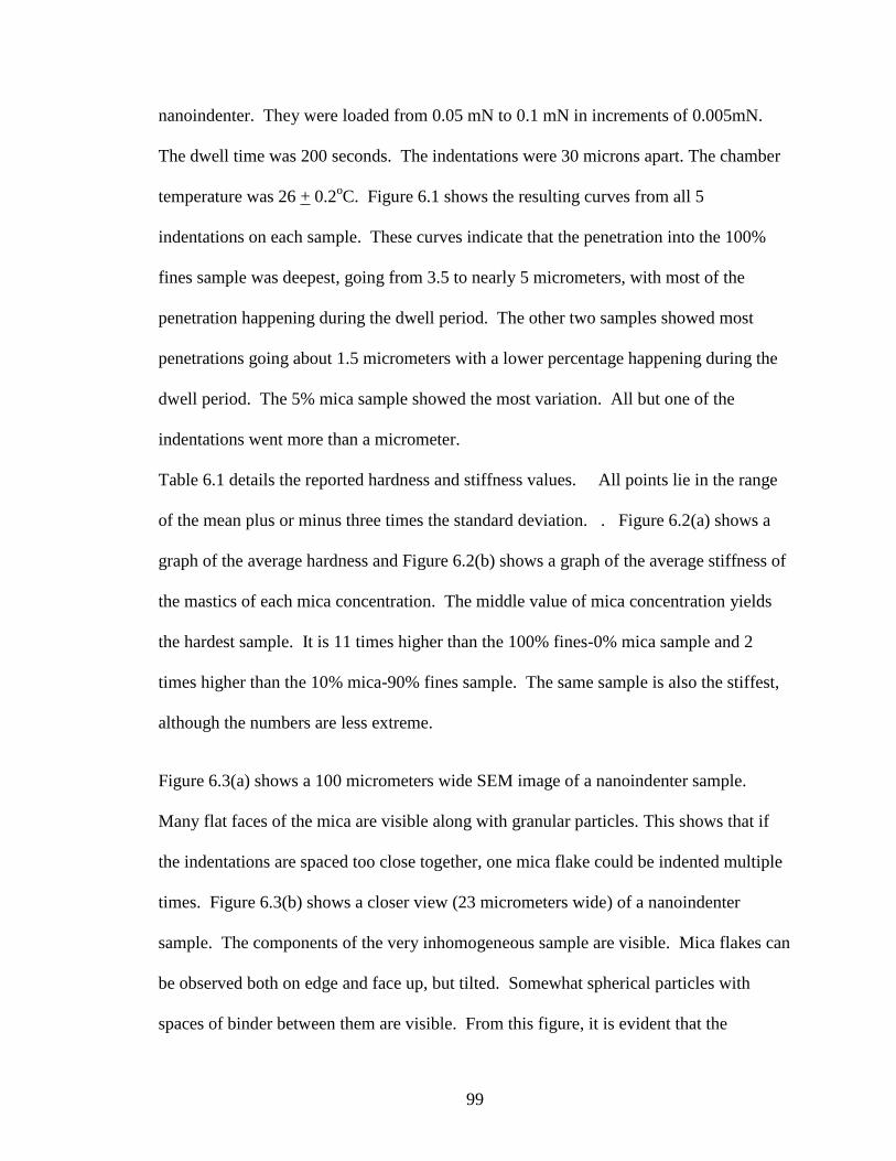
99
nanoindenter. They were loaded from 0.05 mN to 0.1 mN in increments of 0.005mN.
The dwell time was 200 seconds. The indentations were 30 microns apart. The chamber
temperature was 26 + 0.2oC. Figure 6.1 shows the resulting curves from all 5
indentations on each sample. These curves indicate that the penetration into the 100%
fines sample was deepest, going from 3.5 to nearly 5 micrometers, with most of the
penetration happening during the dwell period. The other two samples showed most
penetrations going about 1.5 micrometers with a lower percentage happening during the
dwell period. The 5% mica sample showed the most variation. All but one of the
indentations went more than a micrometer.
Table 6.1 details the reported hardness and stiffness values. All points lie in the range
of the mean plus or minus three times the standard deviation. . Figure 6.2(a) shows a
graph of the average hardness and Figure 6.2(b) shows a graph of the average stiffness of
the mastics of each mica concentration. The middle value of mica concentration yields
the hardest sample. It is 11 times higher than the 100% fines-0% mica sample and 2
times higher than the 10% mica-90% fines sample. The same sample is also the stiffest,
although the numbers are less extreme.
Figure 6.3(a) shows a 100 micrometers wide SEM image of a nanoindenter sample.
Many flat faces of the mica are visible along with granular particles. This shows that if
the indentations are spaced too close together, one mica flake could be indented multiple
times. Figure 6.3(b) shows a closer view (23 micrometers wide) of a nanoindenter
sample. The components of the very inhomogeneous sample are visible. Mica flakes can
be observed both on edge and face up, but tilted. Somewhat spherical particles with
spaces of binder between them are visible. From this figure, it is evident that the
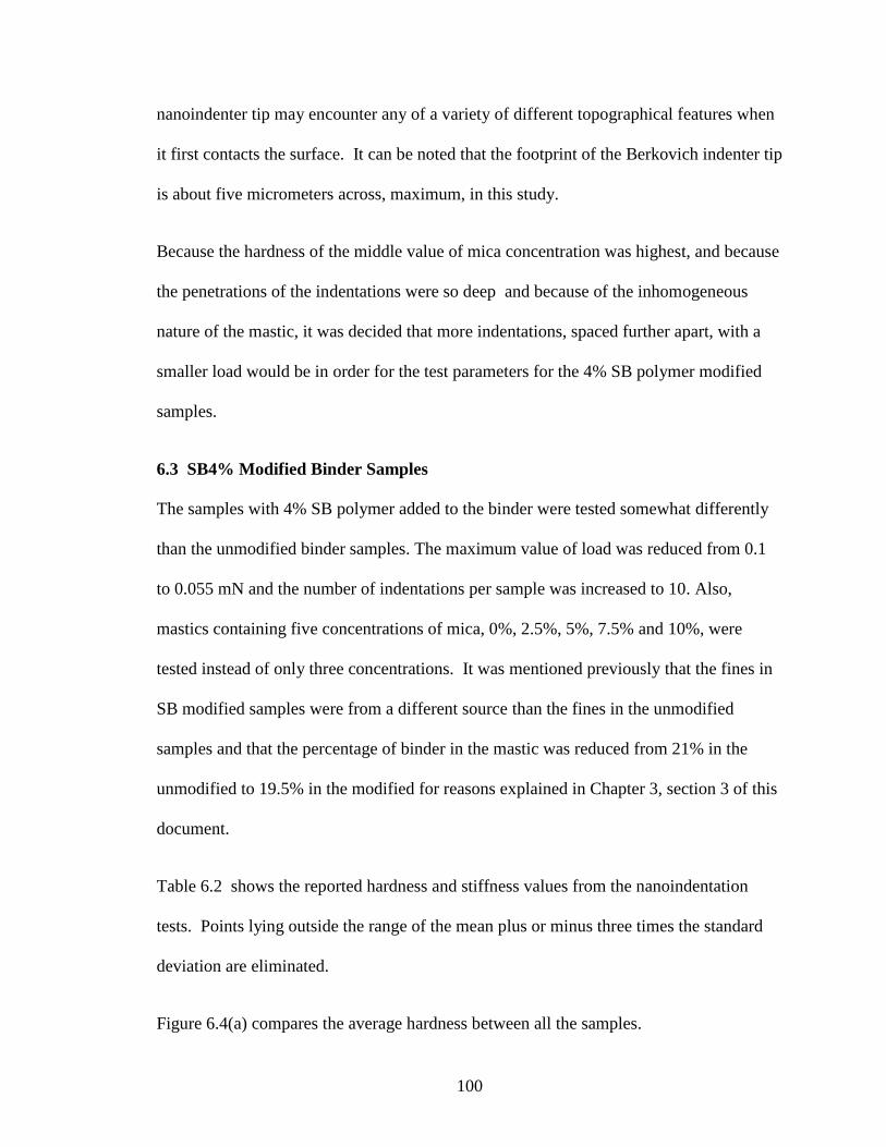
100
nanoindenter tip may encounter any of a variety of different topographical features when
it first contacts the surface. It can be noted that the footprint of the Berkovich indenter tip
is about five micrometers across, maximum, in this study.
Because the hardness of the middle value of mica concentration was highest, and because
the penetrations of the indentations were so deep and because of the inhomogeneous
nature of the mastic, it was decided that more indentations, spaced further apart, with a
smaller load would be in order for the test parameters for the 4% SB polymer modified
samples.
6.3 SB4% Modified Binder Samples
The samples with 4% SB polymer added to the binder were tested somewhat differently
than the unmodified binder samples. The maximum value of load was reduced from 0.1
to 0.055 mN and the number of indentations per sample was increased to 10. Also,
mastics containing five concentrations of mica, 0%, 2.5%, 5%, 7.5% and 10%, were
tested instead of only three concentrations. It was mentioned previously that the fines in
SB modified samples were from a different source than the fines in the unmodified
samples and that the percentage of binder in the mastic was reduced from 21% in the
unmodified to 19.5% in the modified for reasons explained in Chapter 3, section 3 of this
document.
Table 6.2 shows the reported hardness and stiffness values from the nanoindentation
tests. Points lying outside the range of the mean plus or minus three times the standard
deviation are eliminated.
Figure 6.4(a) compares the average hardness between all the samples.
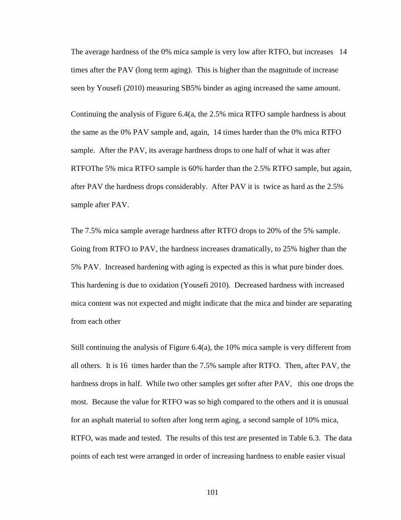
101
The average hardness of the 0% mica sample is very low after RTFO, but increases 14
times after the PAV (long term aging). This is higher than the magnitude of increase
seen by Yousefi (2010) measuring SB5% binder as aging increased the same amount.
Continuing the analysis of Figure 6.4(a, the 2.5% mica RTFO sample hardness is about
the same as the 0% PAV sample and, again, 14 times harder than the 0% mica RTFO
sample. After the PAV, its average hardness drops to one half of what it was after
RTFOThe 5% mica RTFO sample is 60% harder than the 2.5% RTFO sample, but again,
after PAV the hardness drops considerably. After PAV it is twice as hard as the 2.5%
sample after PAV.
The 7.5% mica sample average hardness after RTFO drops to 20% of the 5% sample.
Going from RTFO to PAV, the hardness increases dramatically, to 25% higher than the
5% PAV. Increased hardening with aging is expected as this is what pure binder does.
This hardening is due to oxidation (Yousefi 2010). Decreased hardness with increased
mica content was not expected and might indicate that the mica and binder are separating
from each other
Still continuing the analysis of Figure 6.4(a), the 10% mica sample is very different from
all others. It is 16 times harder than the 7.5% sample after RTFO. Then, after PAV, the
hardness drops in half. While two other samples get softer after PAV, this one drops the
most. Because the value for RTFO was so high compared to the others and it is unusual
for an asphalt material to soften after long term aging, a second sample of 10% mica,
RTFO, was made and tested. The results of this test are presented in Table 6.3. The data
points of each test were arranged in order of increasing hardness to enable easier visual
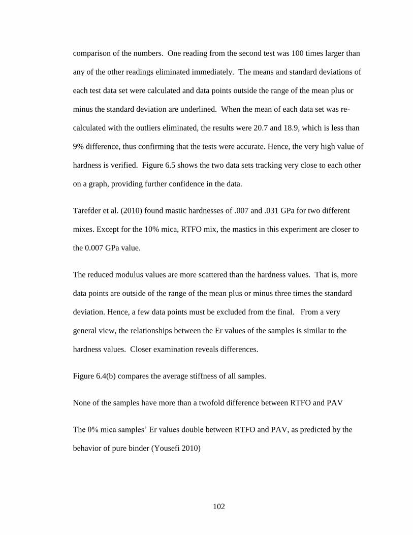
102
comparison of the numbers. One reading from the second test was 100 times larger than
any of the other readings eliminated immediately. The means and standard deviations of
each test data set were calculated and data points outside the range of the mean plus or
minus the standard deviation are underlined. When the mean of each data set was re-
calculated with the outliers eliminated, the results were 20.7 and 18.9, which is less than
9% difference, thus confirming that the tests were accurate. Hence, the very high value of
hardness is verified. Figure 6.5 shows the two data sets tracking very close to each other
on a graph, providing further confidence in the data.
Tarefder et al. (2010) found mastic hardnesses of .007 and .031 GPa for two different
mixes. Except for the 10% mica, RTFO mix, the mastics in this experiment are closer to
the 0.007 GPa value.
The reduced modulus values are more scattered than the hardness values. That is, more
data points are outside of the range of the mean plus or minus three times the standard
deviation. Hence, a few data points must be excluded from the final. From a very
general view, the relationships between the Er values of the samples is similar to the
hardness values. Closer examination reveals differences.
Figure 6.4(b) compares the average stiffness of all samples.
None of the samples have more than a twofold difference between RTFO and PAV
The 0% mica samples’ Er values double between RTFO and PAV, as predicted by the
behavior of pure binder (Yousefi 2010)
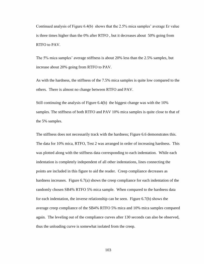
103
Continued analysis of Figure 6.4(b) shows that the 2.5% mica samples’ average Er value
is three times higher than the 0% after RTFO , but it decreases about 50% going from
RTFO to PAV.
The 5% mica samples’ average stiffness is about 20% less than the 2.5% samples, but
increase about 20% going from RTFO to PAV.
As with the hardness, the stiffness of the 7.5% mica samples is quite low compared to the
others. There is almost no change between RTFO and PAV.
Still continuing the analysis of Figure 6.4(b) the biggest change was with the 10%
samples. The stiffness of both RTFO and PAV 10% mica samples is quite close to that of
the 5% samples.
The stiffness does not necessarily track with the hardness; Figure 6.6 demonstrates this.
The data for 10% mica, RTFO, Test 2 was arranged in order of increasing hardness. This
was plotted along with the stiffness data corresponding to each indentation. While each
indentation is completely independent of all other indentations, lines connecting the
points are included in this figure to aid the reader. Creep compliance decreases as
hardness increases. Figure 6.7(a) shows the creep compliance for each indentation of the
randomly chosen SB4% RTFO 5% mica sample. When compared to the hardness data
for each indentation, the inverse relationship can be seen. Figure 6.7(b) shows the
average creep compliance of the SB4% RTFO 5% mica and 10% mica samples compared
again. The leveling out of the compliance curves after 130 seconds can also be observed,
thus the unloading curve is somewhat isolated from the creep.
104
6.4 Conclusions
Generally, the harder a mastic or asphalt concrete is, the more resistant it is to permanent
deformation (rutting). However, as this asphaltic material becomes very hard, it is
subject to cracking. This hardness generally tends to increase with aging, especially when
subjected to cold temperatures. The results of this experiment show that the hardness of
mica-mastic after short term aging increases with mica concentration up to 5% . Above
5% concentration, the behavior is somewhat erratic. First the hardness drops nearly 80%,
and then it increases fifteen fold. Further aging, that is, going from short term (RTFO) to
long term (PAV) aging, yielded varied results. Two samples behaved similarly to those of
Yousefi (2010) as they hardened with age. Three samples softened after long term aging,
with the 10% sample showing the most extreme change. This could suggest that high
concentrations of mica prevents embrittlement or, possibly, that the binder and filler were
separating from each other and the mastic is beginning to crumble.
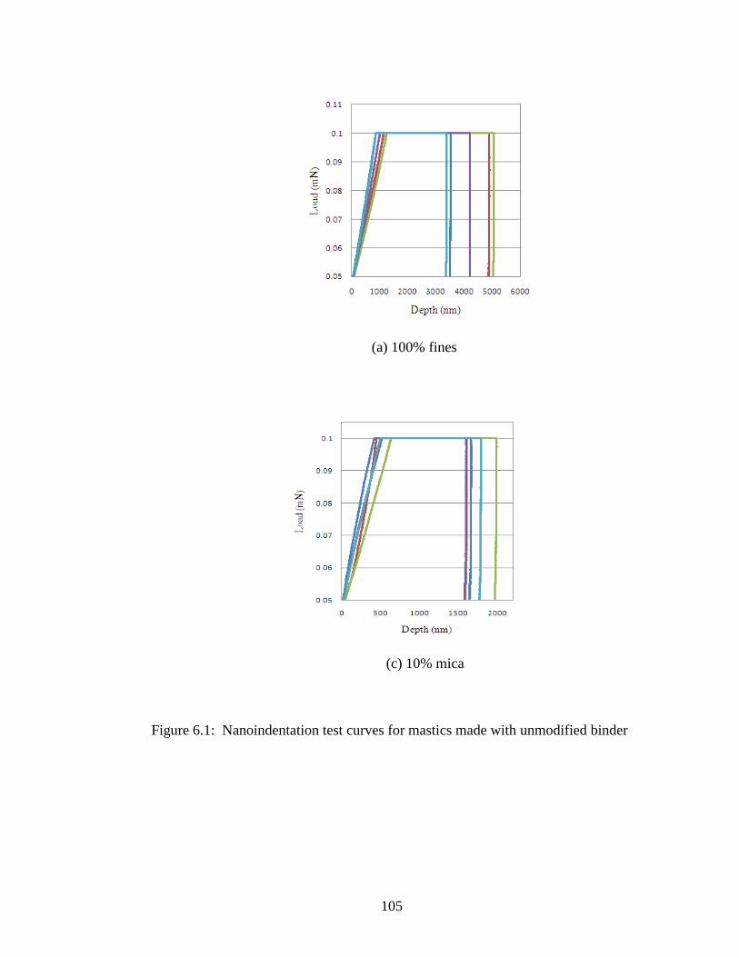
105
(a) 100% fines
(c) 10% mica
Figure 6.1: Nanoindentation test curves for mastics made with unmodified binder
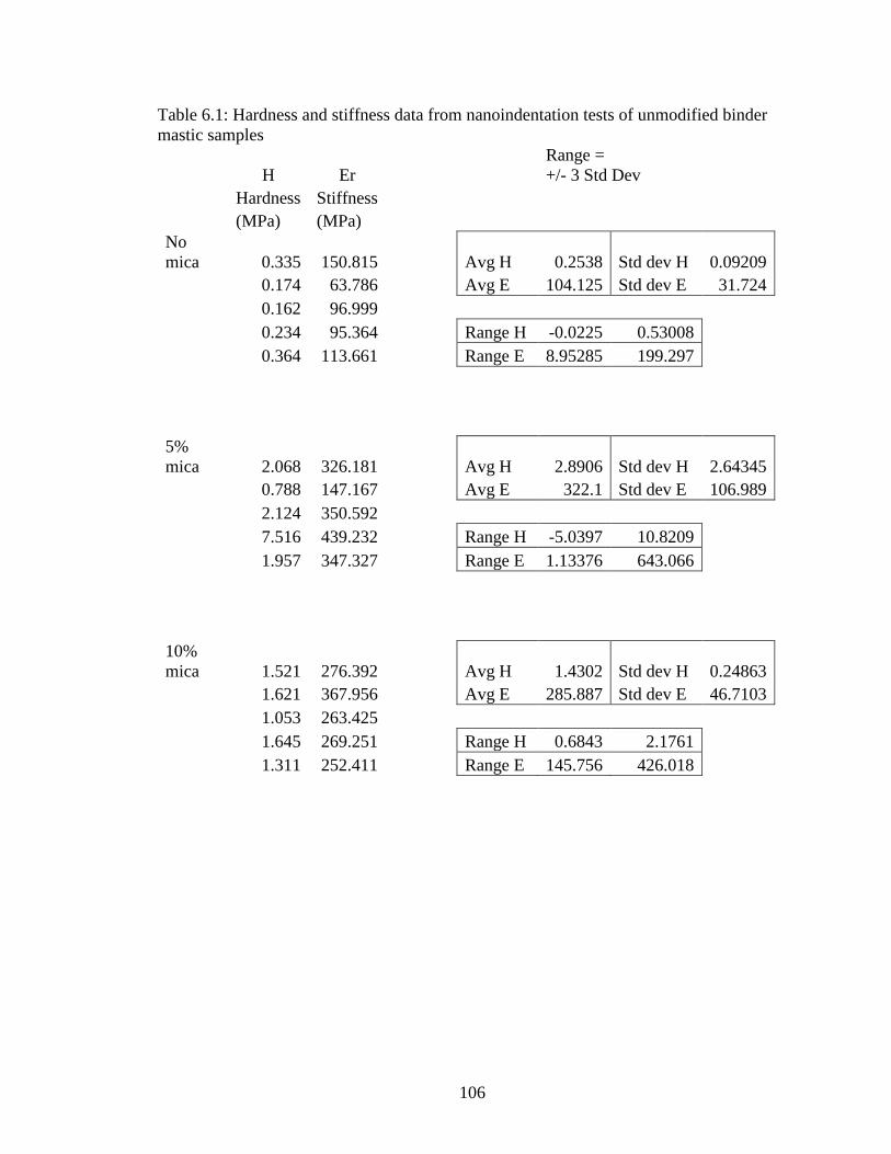
106
Table 6.1: Hardness and stiffness data from nanoindentation tests of unmodified binder
mastic samples
H Er
Range =
+/- 3 Std Dev
Hardness Stiffness
(MPa) (MPa)
No
mica 0.335 150.815
Avg H 0.2538 Std dev H 0.09209
0.174 63.786
Avg E 104.125 Std dev E 31.724
0.162 96.999
0.234 95.364
Range H -0.0225 0.53008
0.364 113.661
Range E 8.95285 199.297
5%
mica 2.068 326.181
Avg H 2.8906 Std dev H 2.64345
0.788 147.167
Avg E 322.1 Std dev E 106.989
2.124 350.592
7.516 439.232
Range H -5.0397 10.8209
1.957 347.327
Range E 1.13376 643.066
10%
mica 1.521 276.392
Avg H 1.4302 Std dev H 0.24863
1.621 367.956
Avg E 285.887 Std dev E 46.7103
1.053 263.425
1.645 269.251
Range H 0.6843 2.1761
1.311 252.411
Range E 145.756 426.018
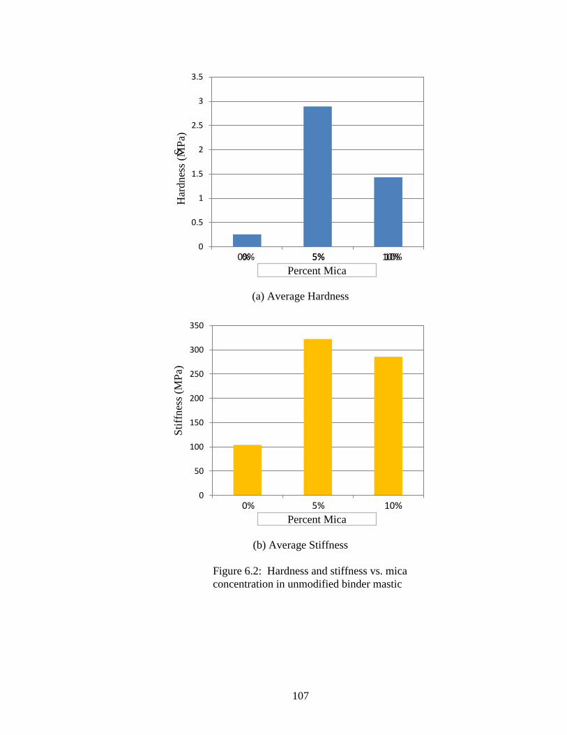
107
(a) Average Hardness
(b) Average Stiffness
0
0.5
1
1.5
2
2.5
3
3.5
1 2 30% 5% 10%
Har
dnes
s (M
Pa)
0% 5% 10%
S
Percent Mica
0
50
100
150
200
250
300
350
1 2 30% 5% 10%
Sti
ffnes
s (M
Pa)
Percent Mica
Figure 6.2: Hardness and stiffness vs. mica
concentration in unmodified binder mastic
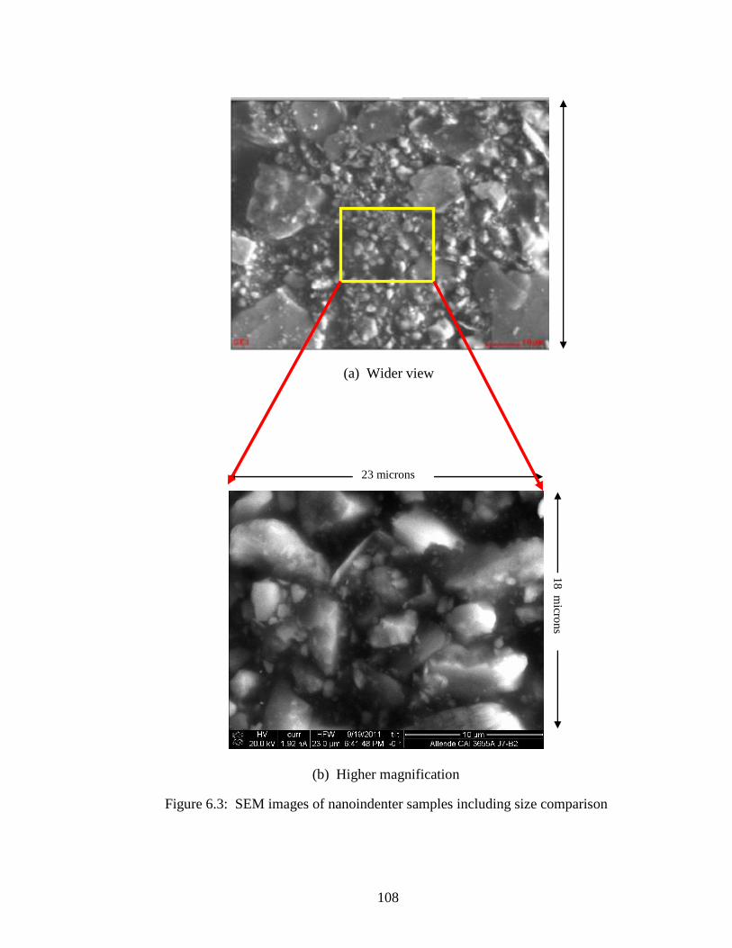
108
(b) Higher magnification
Figure 6.3: SEM images of nanoindenter samples including size comparison
23 microns
18
micro
ns
(a) Wider view
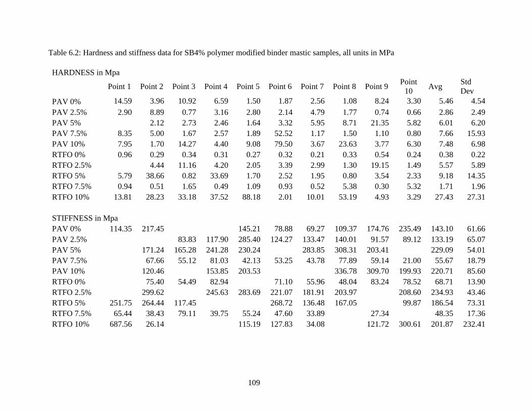
109
Table 6.2: Hardness and stiffness data for SB4% polymer modified binder mastic samples, all units in MPa
HARDNESS in Mpa
Point 1 Point 2 Point 3 Point 4 Point 5 Point 6 Point 7 Point 8 Point 9 Point
10 Avg
Std
Dev
PAV 0% 14.59 3.96 10.92 6.59 1.50 1.87 2.56 1.08 8.24 3.30 5.46 4.54
PAV 2.5% 2.90 8.89 0.77 3.16 2.80 2.14 4.79 1.77 0.74 0.66 2.86 2.49
PAV 5%
2.12 2.73 2.46 1.64 3.32 5.95 8.71 21.35 5.82 6.01 6.20
PAV 7.5% 8.35 5.00 1.67 2.57 1.89 52.52 1.17 1.50 1.10 0.80 7.66 15.93
PAV 10% 7.95 1.70 14.27 4.40 9.08 79.50 3.67 23.63 3.77 6.30 7.48 6.98
RTFO 0% 0.96 0.29 0.34 0.31 0.27 0.32 0.21 0.33 0.54 0.24 0.38 0.22
RTFO 2.5%
4.44 11.16 4.20 2.05 3.39 2.99 1.30 19.15 1.49 5.57 5.89
RTFO 5% 5.79 38.66 0.82 33.69 1.70 2.52 1.95 0.80 3.54 2.33 9.18 14.35
RTFO 7.5% 0.94 0.51 1.65 0.49 1.09 0.93 0.52 5.38 0.30 5.32 1.71 1.96
RTFO 10% 13.81 28.23 33.18 37.52 88.18 2.01 10.01 53.19 4.93 3.29 27.43 27.31
STIFFNESS in Mpa
PAV 0% 114.35 217.45
145.21 78.88 69.27 109.37 174.76 235.49 143.10 61.66
PAV 2.5%
83.83 117.90 285.40 124.27 133.47 140.01 91.57 89.12 133.19 65.07
PAV 5%
171.24 165.28 241.28 230.24
283.85 308.31 203.41
229.09 54.01
PAV 7.5%
67.66 55.12 81.03 42.13 53.25 43.78 77.89 59.14 21.00 55.67 18.79
PAV 10%
120.46
153.85 203.53
336.78 309.70 199.93 220.71 85.60
RTFO 0%
75.40 54.49 82.94
71.10 55.96 48.04 83.24 78.52 68.71 13.90
RTFO 2.5%
299.62
245.63 283.69 221.07 181.91 203.97
208.60 234.93 43.46
RTFO 5% 251.75 264.44 117.45
268.72 136.48 167.05
99.87 186.54 73.31
RTFO 7.5% 65.44 38.43 79.11 39.75 55.24 47.60 33.89
27.34
48.35 17.36
RTFO 10% 687.56 26.14
115.19 127.83 34.08
121.72 300.61 201.87 232.41
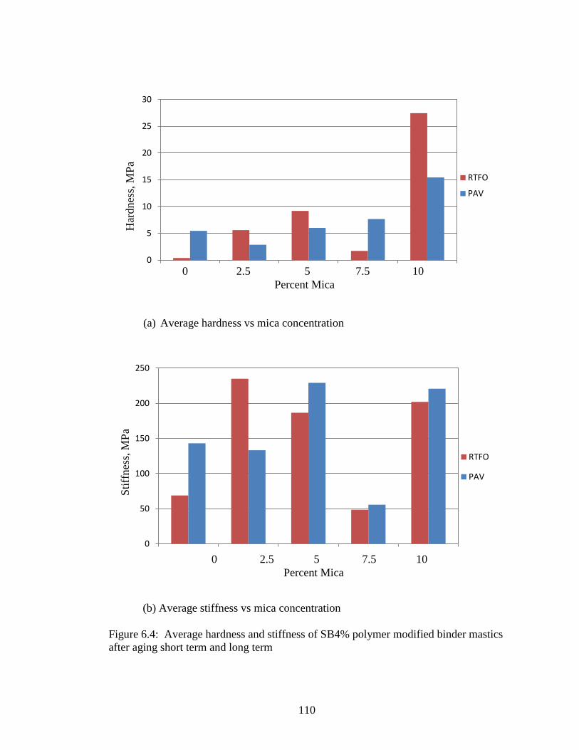
110
(a) Average hardness vs mica concentration
0
5
10
15
20
25
30
1 2 3 4 5
RTFO
PAV
0 2.5 5 7.5 10
Percent Mica
Har
dnes
s, M
Pa
(b) Average stiffness vs mica concentration
Figure 6.4: Average hardness and stiffness of SB4% polymer modified binder mastics
after aging short term and long term
0
50
100
150
200
250
1 2 3 4 5
RTFO
PAV
0 2.5 5 7.5 10
Percent Mica
Sti
ffnes
s,M
Pa
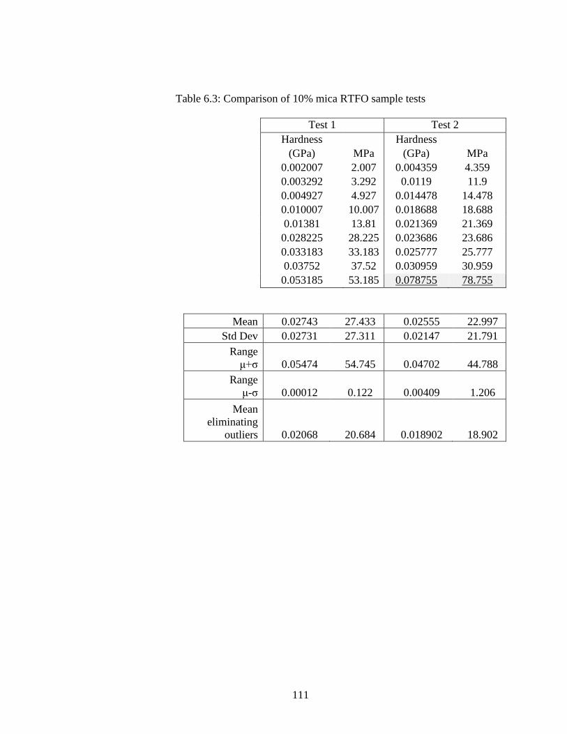
111
Table 6.3: Comparison of 10% mica RTFO sample tests
Test 1 Test 2
Hardness
Hardness
(GPa) MPa (GPa) MPa
0.002007 2.007 0.004359 4.359
0.003292 3.292 0.0119 11.9
0.004927 4.927 0.014478 14.478
0.010007 10.007 0.018688 18.688
0.01381 13.81 0.021369 21.369
0.028225 28.225 0.023686 23.686
0.033183 33.183 0.025777 25.777
0.03752 37.52 0.030959 30.959
0.053185 53.185 0.078755 78.755
Mean 0.02743 27.433 0.02555 22.997
Std Dev 0.02731 27.311 0.02147 21.791
Range
μ+ζ 0.05474 54.745 0.04702 44.788
Range
μ-ζ 0.00012 0.122 0.00409 1.206
Mean
eliminating
outliers 0.02068 20.684 0.018902 18.902
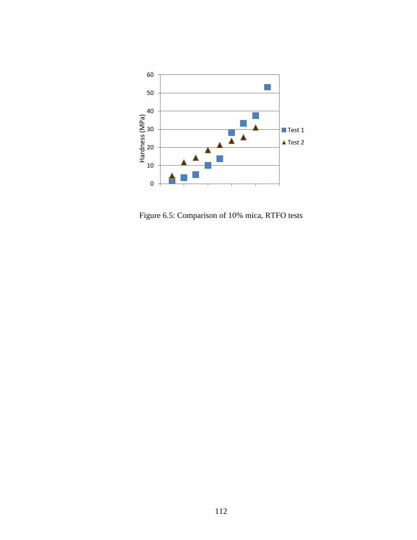
112
Figure 6.5: Comparison of 10% mica, RTFO tests
0
10
20
30
40
50
60
0 2 4 6 8 10
Test 1
Test 2H
ard
nes
s (M
Pa)
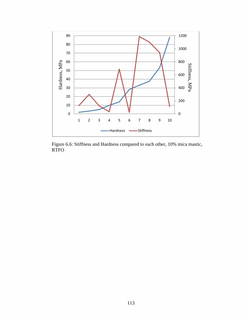
113
Figure 6.6: Stiffness and Hardness compared to each other, 10% mica mastic,
RTFO
0
200
400
600
800
1000
1200
0
10
20
30
40
50
60
70
80
90
1 2 3 4 5 6 7 8 9 10
Har
dnes
s, M
Pa
Hardness Stiffness
Stiffn
ess,M
Pa
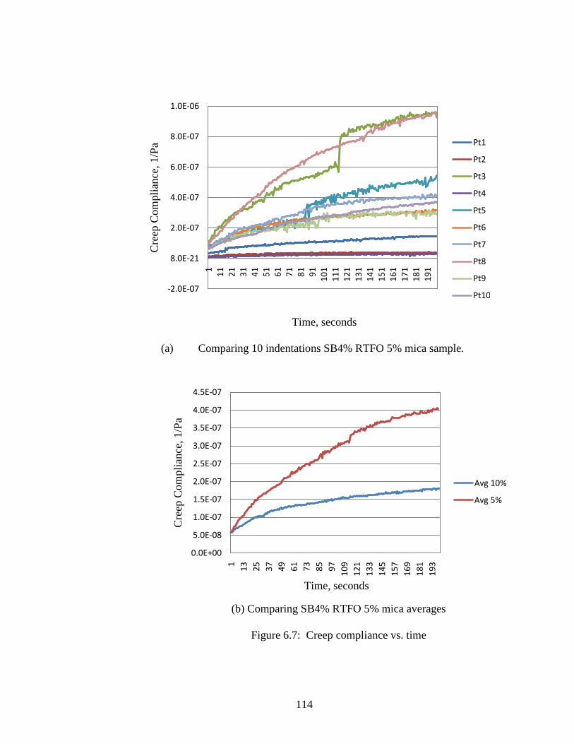
114
(a) Comparing 10 indentations SB4% RTFO 5% mica sample.
-2.0E-07
8.0E-21
2.0E-07
4.0E-07
6.0E-07
8.0E-07
1.0E-06
11
12
13
14
15
16
17
18
19
11
01
11
11
21
13
11
41
15
11
61
17
11
81
19
1
Cre
ep C
om
pli
ance
, 1/P
a Pt1
Pt2
Pt3
Pt4
Pt5
Pt6
Pt7
Pt8
Pt9
Pt10
Time, seconds
(b) Comparing SB4% RTFO 5% mica averages
Figure 6.7: Creep compliance vs. time
0.0E+00
5.0E-08
1.0E-07
1.5E-07
2.0E-07
2.5E-07
3.0E-07
3.5E-07
4.0E-07
4.5E-07
1
13
25
37
49
61
73
85
97
10
9
12
1
13
3
14
5
15
7
16
9
18
1
19
3
Cre
ep C
om
pli
ance
, 1/P
a
Avg 10%
Avg 5%
Time, seconds
115
CHAPTER 7
ANALYSIS OF BENDING BEAM RHEOMETER TESTS ON MASTIC-MICA
7.1 Introduction
In this study, the traditional Bending Beam Rheometer (BBR) test is employed to
characterize the cold temperature stiffness of mastics made with different binders and
containing varying amounts of mica, aged to different levels. In this section, we discuss
the results of the experiments.
7.2 Test Results
During the manufacture of the samples for this test, the difficultly of handling and
compacting mica-fines arose once again. Mixing the binder into the mica-fines took
twice as long as mixing into the pure fines. Also, compacting the mastic into molds took
more energy for the mica-fines and achieving any consistent thickness, let alone the
desired 6.25 mm thickness, was not possible with the compaction method chosen. As the
thickness of the sample is critical in the calculation of stiffness, each sample was
measured with calipers in three locations and the average thickness calculated.
This test was developed for use on binders, which are liquid when molded and sample
compaction and consistent density are not issues. Given the difficulties previously
mentioned, there was concern about inconsistent densities between the samples, so each
sample was weighed and the density calculated. The densities were fairly consistent
between all samples, with most falling between 1.7 g/cm3 and 1.95 g/cm
3 and only one
being particularly high at 2.23 g/cm3. The highest mica concentrations yielded the lowest
densities. The densities of all 24 samples are graphed in Figure 7.1, in which lines are
included between the two samples of each type only to aid the reader. The values are
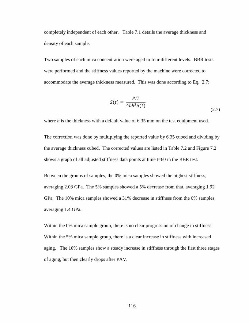
116
completely independent of each other. Table 7.1 details the average thickness and
density of each sample.
Two samples of each mica concentration were aged to four different levels. BBR tests
were performed and the stiffness values reported by the machine were corrected to
accommodate the average thickness measured. This was done according to Eq. 2.7:
(2.7)
where h is the thickness with a default value of 6.35 mm on the test equipment used.
The correction was done by multiplying the reported value by 6.35 cubed and dividing by
the average thickness cubed. The corrected values are listed in Table 7.2 and Figure 7.2
shows a graph of all adjusted stiffness data points at time t=60 in the BBR test.
Between the groups of samples, the 0% mica samples showed the highest stiffness,
averaging 2.03 GPa. The 5% samples showed a 5% decrease from that, averaging 1.92
GPa. The 10% mica samples showed a 31% decrease in stiffness from the 0% samples,
averaging 1.4 GPa.
Within the 0% mica sample group, there is no clear progression of change in stiffness.
Within the 5% mica sample group, there is a clear increase in stiffness with increased
aging. The 10% samples show a steady increase in stiffness through the first three stages
of aging, but then clearly drops after PAV.
117
Figure 7.3 and Figure 7.4 show the stiffness data for times t=120 seconds and t=240
seconds, respectively. The trends are the same as in the t=60 seconds data, but the
stiffness is lower.
7.3 Conclusion
As it has been shown that pure binder shows higher stiffness after aging (Yousefi 2010),
the results of the 0% and 5% sample groups were expected. However, the distinct drop in
stiffness of the 10% sample after long term aging contradicts this. It does confirm the
results of the nanoindentation tests reported in this same study.
The general decrease in stiffness between the sample groups as the mica concentration
increases suggests that high concentrations of mica could help protect asphalt pavement
from the effects of aging. The decrease in stiffness between short and long term aging in
the 10% sample suggests the same thing. As this contradicts conventional thought,
further experiments would be required before such a claim could be made.
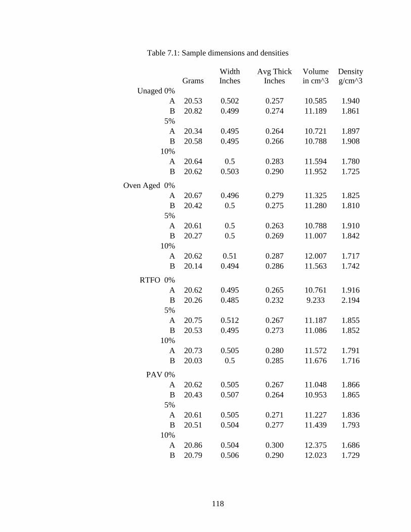
118
Table 7.1: Sample dimensions and densities
Grams
Width
Inches
Avg Thick
Inches
Volume
in cm^3
Density
g/cm^3
Unaged 0%
A 20.53 0.502 0.257 10.585 1.940
B 20.82 0.499 0.274 11.189 1.861
5%
A 20.34 0.495 0.264 10.721 1.897
B 20.58 0.495 0.266 10.788 1.908
10%
A 20.64 0.5 0.283 11.594 1.780
B 20.62 0.503 0.290 11.952 1.725
Oven Aged 0%
A 20.67 0.496 0.279 11.325 1.825
B 20.42 0.5 0.275 11.280 1.810
5%
A 20.61 0.5 0.263 10.788 1.910
B 20.27 0.5 0.269 11.007 1.842
10%
A 20.62 0.51 0.287 12.007 1.717
B 20.14 0.494 0.286 11.563 1.742
RTFO 0%
A 20.62 0.495 0.265 10.761 1.916
B 20.26 0.485 0.232 9.233 2.194
5%
A 20.75 0.512 0.267 11.187 1.855
B 20.53 0.495 0.273 11.086 1.852
10%
A 20.73 0.505 0.280 11.572 1.791
B 20.03 0.5 0.285 11.676 1.716
PAV 0%
A 20.62 0.505 0.267 11.048 1.866
B 20.43 0.507 0.264 10.953 1.865
5%
A 20.61 0.505 0.271 11.227 1.836
B 20.51 0.504 0.277 11.439 1.793
10%
A 20.86 0.504 0.300 12.375 1.686
B 20.79 0.506 0.290 12.023 1.729
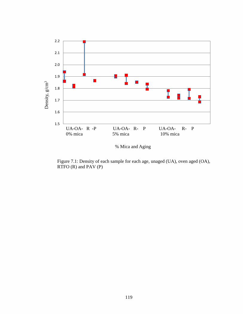
119
Figure 7.1: Density of each sample for each age, unaged (UA), oven aged (OA),
RTFO (R) and PAV (P)
1.5
1.6
1.7
1.8
1.9
2.0
2.1
2.2
0 2 4 6 8 10 12 14
Den
sity
, g/c
m3
% Mica and Aging
UA-OA- R -P UA-OA- R- P UA-OA- R- P
0% mica 5% mica 10% mica
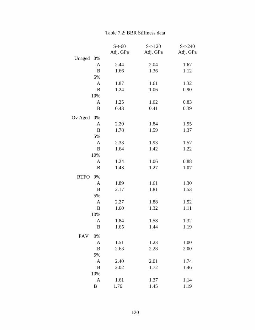
120
Table 7.2: BBR Stiffness data
S-t-60
Adj. GPa
S-t-120
Adj. GPa
S-t-240
Adj. GPa
Unaged 0%
A 2.44 2.04 1.67
B 1.66 1.36 1.12
5%
A 1.87 1.61 1.32
B 1.24 1.06 0.90
10%
A 1.25 1.02 0.83
B 0.43 0.41 0.39
Ov Aged 0%
A 2.20 1.84 1.55
B 1.78 1.59 1.37
5%
A 2.33 1.93 1.57
B 1.64 1.42 1.22
10%
A 1.24 1.06 0.88
B 1.43 1.27 1.07
RTFO 0%
A 1.89 1.61 1.30
B 2.17 1.81 1.53
5%
A 2.27 1.88 1.52
B 1.60 1.32 1.11
10%
A 1.84 1.58 1.32
B 1.65 1.44 1.19
PAV 0%
A 1.51 1.23 1.00
B 2.63 2.28 2.00
5%
A 2.40 2.01 1.74
B 2.02 1.72 1.46
10%
A 1.61 1.37 1.14
B 1.76 1.45 1.19
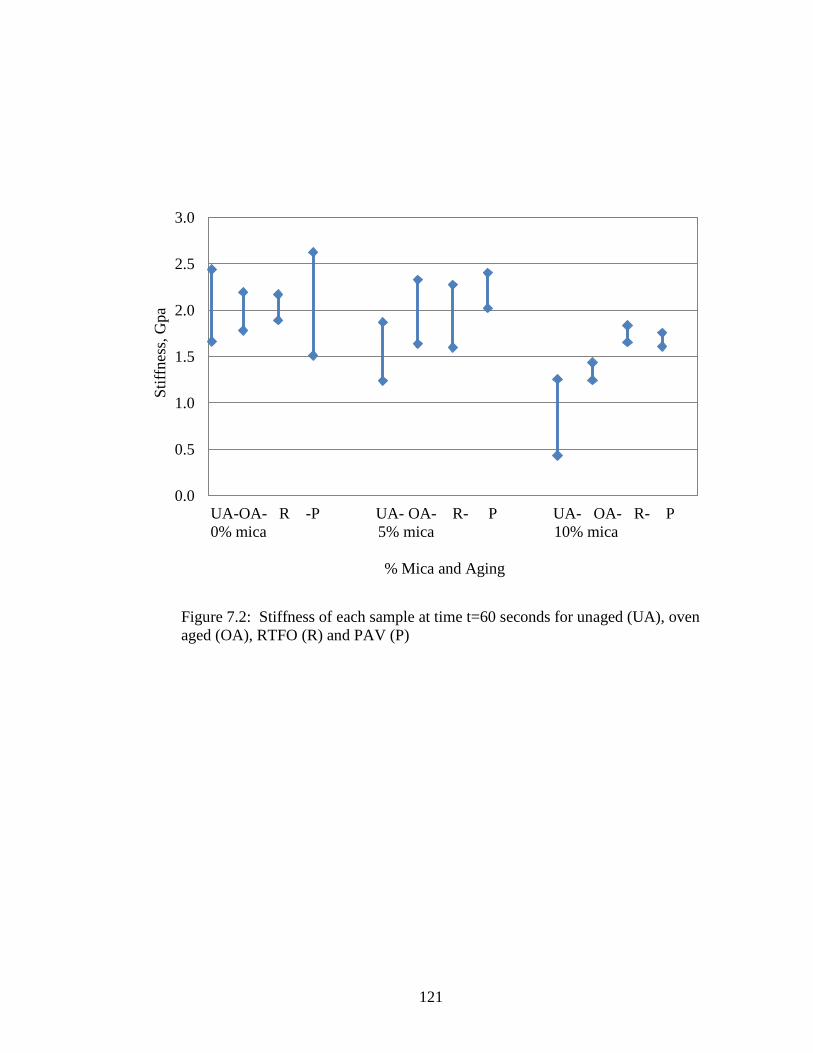
121
Figure 7.2: Stiffness of each sample at time t=60 seconds for unaged (UA), oven
aged (OA), RTFO (R) and PAV (P)
0.0
0.5
1.0
1.5
2.0
2.5
3.0
0 2 4 6 8 10 12 14
Sti
ffnes
s, G
pa
UA-OA- R -P UA- OA- R- P UA- OA- R- P
0% mica 5% mica 10% mica
% Mica and Aging
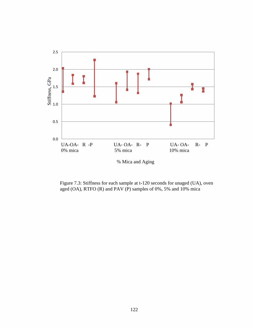
122
Figure 7.3: Stiffness for each sample at t-120 seconds for unaged (UA), oven
aged (OA), RTFO (R) and PAV (P) samples of 0%, 5% and 10% mica
0.0
0.5
1.0
1.5
2.0
2.5
0 2 4 6 8 10 12 14
Sti
ffnes
s, G
Pa
UA-OA- R -P UA- OA- R- P UA- OA- R- P
0% mica 5% mica 10% mica
% Mica and Aging
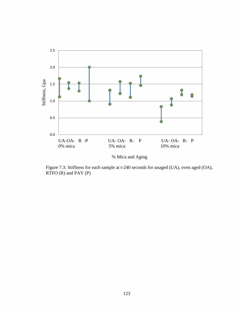
123
Figure 7.3: Stiffness for each sample at t-240 seconds for unaged (UA), oven aged (OA),
RTFO (R) and PAV (P)
0.0
0.5
1.0
1.5
2.0
2.5
0 2 4 6 8 10 12 14
Sti
ffnes
s, G
pa
UA-OA- R -P UA- OA- R- P UA- OA- R- P
0% mica 5% mica 10% mica
% Mica and Aging
124
CHAPTER 8
CONCLUSION
8.1 Introduction
In this investigation we have studied the effects of mica on asphalt aging, that is, the
stiffening of asphalt due to high temperatures (as would occur during road construction)
and long term exposure to the elements. We have shown, at micro and macro scales, that
the presence of mica does affect the final performance of mastic, particularly if the mica
is 5% or more of the total weight of the aggregate fines. We identified and roughly
quantified the presence of mica in the mineral fines, that is, we were able to identify
relative concentrations of mica in mineral fines. We measured the hardness and stiffness
at a micro scale and the stiffness at a macro scale. We observed and analyzed the
material after fracture occurred.
Generally, the harder or stiffer a mastic or asphalt concrete is, the more resistant it is to
rutting. However, as this asphalt becomes very hard, it is subject to cracking of all types
under traffic load (Lee et. al 2007).
8.2 XRD
Sample preparation is critical for the XRD. The method used was chosen because the
content and particle sizes were known and it was desired to demonstrate the behavior of
the entire bulk of the fines portion of the aggregate.
The areas of the different mica peaks in the XRD diffraction patterns could be useful in
developing a relationship between the patterns and the amounts of the phases present.
However, use of this method for quantification can be significantly affected by the
125
tendency of mica to lie in a preferred, ordered orientation, thus amplifying the intensity of
well oriented peaks and attenuating that of other peaks. The method in which these
samples were prepared allowed for a high degree of particle orientation. Diffraction
patterns of five samples of the same fines with varied concentrations of mica were
compared to one another and the differences trended with mica concentration. A sample
from a different fines source with a known concentration of mica added yielded a very
different XRD pattern which would not have allowed for prediction of the mica content.
In such a material as aggregate fines, with so many possible materials (phases), each of
unknown quantity, causing unknown overlapping peaks in the XRD pattern,
quantification requires deconstruction, or deconvolution, of the overlaps to obtain reliable
peak areas. XRD machines do have the software required for this. Still, the platy shape
of the mica flake would tend to cause orientation and exaggerate the peaks artificially.
A more common method of preparing samples for Powder XRD is to extract fines that
remain suspended in water and deposit them on the glass slide. This yields a sample with
much smaller particles, ideally, 1 micron size. While this method did not serve the needs
of this experiment, it could be developed as a method to use for analyzing aggregate from
the field.
8.3 SEM
Generally, the mastics with concentrations of mica greater than 5% were very dry and
difficult to handle and mold. Keeping the weight percentage of binder constant with
increasing percentages of mica yielded very different mastics. This detail was the most
dominant characteristic observed in all of the experiments. Observation in the SEM
126
showed so many flakes that were either un-coated or only lightly coated that it was
difficult to analyze.
The most dominant characteristic viewed in the SEM was that there were more uncoated
flakes seen in holes and cracks than on flat, stable areas, regardless of the aging. The
largest fractured surfaces were produced by experimenters forcing the fracture, but some
small pieces would crumble off the main surface “voluntarily.” The surfaces of the
crumbles revealed high concentrations of uncoated mica, suggesting that breakage is
caused by mica separating from the mastic.
As the aging increased from unaged to oven aged to RTFO to Post-PAV, there was a
small, inconsistent increase in the number of un-coated flakes seen in the SEM. The
samples molded Pre-PAV had the highest number of uncoated flakes, by a small amount.
8.4 Nanoindention
The hardness of the samples, as measured by nanoindention, produced some results that
contradicted expectations. Increased aging from short-term aging (RTFO) to long term
aging (PAV) was expected to show increased hardness, and, therefore, increased fragility,
as pure binder does. The “no mica” sample of mastic did as expected. The addition of
mica, even low concentrations, dramatically changed the amount of response, both after
short term and long term aging. The hardness increased overall for 2.5% and 5%, then
decreased for 7.5%. However, it was lower after PAV than RTFO for 2.5% and 5%.
This contradicts the expectations of “hardness increases with aging.” At 10% mica, the
behavior was completely contrary to all other data. The hardness after RTFO was much
higher than any other sample, then it decreased 50% going from RTFO to PAV. This
127
could suggest that a high concentration of mica prevents age damage, or, possibly, that
the binder and filler were separating from each other and the mastic is beginning to
crumble.
8.5 Bending Beam Rheometer
This test is designed to determine the response of an asphalt material responds to cold
temperatures. The flexural creep stiffness measured is considered to be a reliable
indicator of pavement brittleness in cold weather.
It has been shown that pure binder shows higher stiffness after aging and the results of
the 0% and 5% sample groups in this experimented followed that trend . However, there
is a distinct drop in stiffness of the 10% sample after long term aging that contradicts this
trend. Also, there is a general decrease in stiffness between the sample groups as the
mica concentration increases, suggesting that high concentrations of mica could help
protect asphalt pavement from the effects of aging. The aforementioned results for the
10% sample suggest the same thing. As this contradicts conventional thought, further
experiments would be required before such a claim could be made. These results do
confirm the results of the nanoindentation tests reported in this same study.
8.6 Conclusions
Mica concentrations in fines can be detected and, to an extent, quantified with
XRD.
Mica absorbs much more binder than fines.
Cracks in mastic tend to follow uncoated mica flakes.
128
The number of uncoated mica flakes increases dramatically with mica content and
slightly with aging. There is no consistent difference between unmodified and
modified binder.
At a micro scale, hardness decreases with increasing mica content. At 10% mica
concentration, hardness decreases with long term aging.
At a macro scale, at cold temperatures, the stiffness decreases at 10% mica
concentrations and, similar to the micro scale results, decreases after long term
aging.
8.7 Recommendations
The test results of the 10% mica samples in the nanoindenter and the BBR require
further experiments with more samples for confirmation or refutation.
There was no moisture conditioning done in the aging processes in this
experiment.
XRD testing on many fines sources with mica added, using only one micrometer
size particles, would allow for development of reliable methods.
129
REFERENCES
AASHTO Test Procedure R 28-06: Accelerated Aging of Asphalt Binder Using a
Pressurized Aging Vessel (PAV). American Association of State Highway and
Transportation Officials, Washington, D. C., 2006
AASHTO Test Procedure T 240-06: Effect of Heat and Air on a Moving Film of Asphalt
(Rolling Thin-Film Oven Test). American Association of State Highway and
Transportation Officials, Washington, D. C., 2006
AASHTO Test Procedure T 313-08: Determining the Flexural Creep Stiffness of Asphalt
Binder Using the Bending Beam Rheometer (BBR). American Association of State
Highway and Transportation Officials, Washington, D. C., 2008
Anderson, D.A., Bahia, H.U. and Dongre, R. (1992), “Rheological Properties of Mineral
Filler – Asphalt mastics and Their Relationship to Pavement Performance.” Effects of
Aggregates and Mineral Fillers on Asphalt Mixture Performance: ASTM STP 1147.
Richard C. Meininger, editor, American Society for Testing and Materials, Philadelphia.
Anderson, D. A., Bonaquist, R., “NCHRP Report 709 Investigation of Short-Term
Laboratory Aging of Neat and Modified Asphalt Binders.” Transportation Research
Board, Washington, D.C., 2012.
130
Beake, B., Goodes, S., Jones, S., Gray, A., Harris, A., Pickford, N., Smith, J., “NanoTest
Online Help File Version 1.0 and NanoTest Manual Version 3.0.” Micro Materials Ltd,
Wrexham, United Kingdom, 2006
Chakrapani, G. J., Subramanian, V., Gibbs, R. J., “Size Characteristics and Mineralogy of
Suspended Sediments of the Ganges River, India.” Environmental Geology, Vol. 25,
Issue 3, 1995, pp 192-196
Dolley, T. P. (2008), “Mica.” United States Geological Survey 2008 Minerals Yearbook,
U. S. Department of the Interior, July 2010.
Dufek, M., (2008) “Quanta 3D FEG User Operation Manual, 4th
Edition.” FEI
Company, published electronically.
Fischer-Cripps, A. C. (2002) “Nanoindentation.” Mechanical Engineering Series, 2nd
Edition, Springer Science Media, LLC, New York.
Huang, B., Shu, X., Chen, X. (2007), “Effects of mineral fillers on hot-mix asphalt
laboratory-measured properties.” International Journal of Pavement Engineering. Vol. 8,
No. 1, pp 1-9.
JEOL Ltd. (2006), “Invitation to the SEM World” Informational Brochure No.
118C496(Ks), JEOL Ltd., 1-2 Musashino 3-chome Akshima Tokyo 196-8558.
Kandhal, P. S., Lynn, C. Y., Parker, Jr, F. (1998), “Characterization Tests for Mineral
Fillers Related to Performance of Asphalt Paving.” National Center for Asphalt
Technology of Auburn University”, NCAT Report No. 98-2.
131
Kandhal, P. S., Lynn, C. Y., Parker, F. (1998), “Tests for Plastic Fines in Aggregates
Related to Stripping in Asphalt Paving Mixtures.” National Center for Asphalt
Technology of Auburn University”, NCAT Report No. 98-3.
Kandhal, P. and Parker, F., Jr. (1998), “NCHRP Report 405 Aggregate Tests Related to
Asphalt Concrete Performance in Pavements.” Transportation Research Board, National
Academy Press, Washingon, D.C., 1998, 103 p.
Kleijn, W. B., Oster, J. D. (1982), “A Model of Clay Swelling and Tactoid Formation.”
Clays and Clay Minerals, Vol. 30, No. 5, pp 383-390.
Klein, C., Hurlbut, C. S., Jr. (1993), “Manual of Mineralogy (after James D. Dana),”
John Wiley & Sons, Inc. New York.
Lamond, J. F., Pielert, J. H. (2006), “Significance of Tests and Properties of Concrete
and Concrete-Making Materials STP 169D,” ASTM International, West Conshohocken
PA.
Lee, S.J., Amirkhanian, S. N., Shatanawi, K., Kim, K, “Short-term aging characterization
of asphalt binders using gel permeation chromatography and selected Superpave binder
tests.” Construction and Building Materials, 2007,
doi:10.1016/j.conbuildmat.2007.08.005
Kondelchuk, D., Miskovsky, K. (2008), “Determination of the Test Methods Sensitive to
Free Mica Content in Aggregate Fine Fractions.” Journal of Materials Engineering and
Performance. Vol. 18, No. 3, pp. 282-286
132
Miskovsky, K. (2004), “Enrichment of fine mica originating from rock aggregate
production and its influence on the mechanical properties of bituminous mixtures.”
Journal of Materials Engineering and Performance. 2004, Vol. 13, Iss. 5, ISSN: 1059-
9495, pp. 607-611.
Ries, H. (1898), “The Origin of Kaolin.” Transactions f the American Ceramic Society
First Annual Meeting, Society Secretary’s Office, Columbus, OH, Jan 10, 1900, pp 93-
99.
Roberts, F.L., Kandhal, P.S., Brown, E.R., Lee, D.Y., Kennedy, T.W., “Hot Mix
Asphalt Materials, Mixture Design, and Construction, Second Edition”. National Asphalt
and Pavement Association Research and Education Foundation, Lanham, Maryland,
1991.
Said, S. F., Loorents, K. J., and Hakim, H. (2009), “Impact of mica content on water
sensitivity of asphalt concrete.” International Journal of Pavement Engineering.
February 2009, Vol. 10, No. 1, pp 1- 8.
Schields, P. J., “Bragg's Law and Diffraction: How waves reveal the atomic structure of
crystals.” Center for High Pressure Research, Department of Earth & Space Sciences,
State University of New York at Stony Brook. Website visited many times between
October 2010 and October 2011:
http://www.bmsc.washington.edu/people/merritt/bc530/bragg/
133
Tarefder, R. A., Zaman, A. M., Uddin, W. (2010), “Determining Hardness and Elastic
Modulus of Asphalt by Nanoindentation.” International Journal of Geomechanics.
Volume 10 Issue 3, May/June 2010, pp. 106-116.
United States Department of the Interior Bureau of Land Management (BLM 2006)
Surface Management Topographic Map, Chama, New Mexico. Available online.
Wang, H., Al-Qadi, I. L., Faheem, A. F., Bahia, H. U., Yang, S. and Reinke, G. H.
(2011), “Effect of Mineral Filler Characteristics on Asphalt Mastic and Mixture Rutting
Potential.” Proceedings Transportation Research Board Annual Meeting 2011, 14 pages.
Welton, J. E. (1984), “SEM Petrology Atlas.” Chevron Oil Field Research Company,
Methods in Exploration Series, The American Association of Petroleum Geologists,
Tulsa, OK, USA
White, T. D., Haddock, J. E., Rismantojo, E. (2006), “NCHRP Report 557 Aggregate
Tests for Hot-Mix Asphalt Mixtures Used in Pavements.” Transportation Research
Board.
Willmer, A. J., Maxwell, T. D. (1993), “Archaeological Survey of Mica Mines in the
Apache-Cribbenville District, Petaca Mining Region, Rio Arriba County, New Mexico.”
Archaeology Notes 114, Museum of New Mexico, Office of Archaeological Studies, Santa
Fe, NM. 1993.
Website: Mindat.org. Online database of minerals. Visited many times between June
and October 2011.
134
Woodward, D., Woodside, A., Jellie, J.(2002), “Clay in Rocks.” Society of Chemical
Industry Lecture Paper Series, ISSN 1353-114X.
Yousefi, S. S. (2010), “Rheological and Nanomechanical Characterization of Aging in
Polymer Modified Asphalt.” Master’s Thesis, University of New Mexico Civil
Engineering, November 2010.
135
APPENDIX I
The following pages summarize the observations made on the SEM. View sizes are
approximate, mica flakes counted are between 20 and 75 micrometers across the face
(i.e., if the flake was round, its diameter would measure between 20 and 75 micrometers).
Attempts to measure the areas of the visible mica flakes were discarded due to the
presence of many flakes presenting only edge views, which prevented realistic estimation
of their areas.
Key of chemical formulas:
C is carbon Si is silicon Al is aluminum
Ca is calcium O is oxygen Fe is iron
K is potassium S is sulfur
Unmodified pre PAV
0% Images of rough and smooth areas yielded similar EDX spectra of Al and Si in
peaks that could be muscovite or illite, but no K peak. Also a very strong Ca
peak.
2.5% Much Ca in EDX.
o 5.1 mm view, no flakes
o 0.5 mm Flat area near hole had 11 large flakes showing.
o 0.5 mm Bottom of same hole showed 5 flakes, no EDX signal
o 0.9 mm view, disturbed, breaking area 15 flakes
o 0.3mm view, flat, stable, near edge, 3 flakes, EDX slow, a lot of Ca.
136
5% Much Ca in EDX. Some sulfur.
o 4.6 mm view, deep hole, no flakes. Entire sample has holes and unstable
o 0.78 mm flattish area near hole, 11 flakes
o 0.64 mm, no flakes. In a hole. Maybe many slightly coated. Not real clear.
7.5% Much Ca in EDX. Some sulfur.
o 5.1 mm view, no flakes, very rough and hilly
o .76 mm view, flat area, many flakes visible, confirmed 28
o .53 mm view, in a hole, similar to flat area, confirmed 16 flakes
o .33 mm view, flat area, similar, 10 flakes
10% Ca peak as tall as C peak. Si almost as tall.
o 1.3 mm view, rough area, innumerable flakes, coated and uncoated.
o .6 mm view, another rough area, innumerable flakes, coated and uncoated.
o .9 mm view, flat, stable area near edge, , innumerable flakes, coated and
uncoated.
137
Unmodified Post PAV
0% 1.2 mm view mostly smooth and black with very bright white particles on top.
EDX shows C dominating at more than 3x any other element. Focus on a
white particle shows O and Si peaks increasing some.
o 1.3 mm view zooms in on white area on surface. It appears to be a regular
part of the binder catching the electron beam at an odd angle compared to
the surrounding area. No EDX spectrum rose.
2.5% 1 mm view shows many white lines over the entire sample. No mica flakes
found. EDX shows strong C peak, weak O peak and all others too weak to
consider.
5% Many white “ridges” over entire image. Seems to be binder.
o .1 mm view shows close-up of white ridge. Not clear what it is. EDX
shows strong C, weak O and nothing else of significance.
o .05 mm view shows 1 flake with strong EDX confirming mica. Much
searching of the sample revealed only a few of these.
7.5% Mostly flat.
o 0.72 mm view of a flat area shows at least 5 flakes. EDX shows very
strong C with weak mica peaks
o .18 mm view shows 7 flakes occupying 80% of area. Mica peaks are very
strong in the EDX.
10% Mostly flat
o 1.13 mm view shows many shapes that could be mica. EDX shows mica
peaks increasing with zoom in to smaller areas.

138
o .35 mm view shows a single flake occupying about 50% of the area. The
EDX shows very strong mica peaks.
139
Unmodified RTFO
0% 4.6 mm view has “smooth hill” with a large crack in it. EDX shows some Si,
Al and O with a small amount of K. There is a lot of Ca and some S.
o .56 mm view shows a rough surface and the EDX is very similar to the
wider view.
o .09 mm view continued the zoom in to the same spot. Particles under 1
micrometer are visible. EDX similar except Al peak is shorter. Ca still
quite high.
o .9 mm view, random flat area, rough surface, no flakes, same EDX
o .143 mm view, down a hole, possible flakes, coated.
2.5% Still much Ca in EDX, little K
o 2.55 mm view, mixed topography, hole and flat area,
o 1.7 mm view, general search of area, including zooms-in no mica
uncoated
o .82 mm view, in hole, no uncoated flakes visible
o .26 mm view, deep in a hole, 10 bare flakes found
5% Much searching of entire sample, including many zoom-ins and 8 images
taken, found only 3 pockets of flakes.
o .35 mm view had 16 flakes
o .19 mm view had 4 flakes
o .465 mm view had 10 unconfirmed flakes, very deep in a hole
7.5% 6.8 mm view included flat area, hole, broken pieces. Spectrum very slow to
rise.
140
o 1.2 mm view, looking into hole, appears to be 80% uncoated mica.
o .91 mm view, flat area, innumerable flakes, about 70%. Zoom-ins
appeared as uncoated mica. Images were taken of wider areas to give
sense of magnitude. Strong spectrum peaks.
10% .95 mm view looking down a hole, 100% flakes. EDX shows very strong Ca
peak, almost as strong as the C. However, EDX of a single flake shows weak
Ca and much stronger Si.
o .3 mm view shows grains of Ca in among the flakes. It all looks quite dry,
uncoated but the C peak remains steady, if not dominant.
141
Unmodified Oven aged
0% A few mica flakes were found in the sample. The EDX spectra showed strong
Si peaks, some weak Al peaks and very weak K peaks. Some of the images
show edges that could be mistaken for coated mica flakes. See Figure 4.13.
2.5% The sample had a rugged surface with many “hills and valleys” and cracks.
o mm view, looking down a slope, showed innumerable flake shapes, 16
confirmed uncoated. On the flatter side of the sample, no uncoated flakes
were visible. EDX of different flakes showed very different spectra.
o .99 mm view, rugged area with holes. 1 large flake absolutely uncoated.
Many flake shapes probably uncoated. Very difficult to say for certain
without examining every flake at very high magnification.
o .19 mm view, zoom-in on one flake from the .99 mm view. Very strong
Si and Al peaks, good K peak. See Figure 4.12(a) and (b).
o .92 mm view, in a hole, 12 flakes
o .96 mm view, on a flat area, 5 flakes.
5% First impressions of this sample were that it had too few un-coated mica flakes
and the Ca peaks were very high. It was so extreme that a second sample was
prepared and examined.
o .186 mm view, EDX of what appears to be coated mica returns strong Al,
Si, K and O peaks.
o 1.43 mm view, generally flaky appearance. EDX of the entire area and
smaller areas all gave strong muscovite peaks. The Ca peak is very high.
142
o .49 mm view, in a hole, 18 flakes clearly visible with more sticking out the
side of the hole. Zoom-out from the hole, it appears to be about 20%
flakes. Very difficult to count.
o .8 mm view, near another hole. Near the hole, there are at least 10
uncoated flakes. Away from the hole, the flakes appear coated. Very
strong mica peaks, Ca strongest seen thus far, especially on some
individual flakes.
o Second sample, .58 mm view, on a break, innumerable flakes. On a flat,
many coated flakes, some area show no flakes, the Ca peak is very high.
7.5% Sample appears to have a mostly stable surface with a large flat area and some
holes and breaks.
o 5 mm view, EDX shows strong mica peaks and a lot of Ca in whole area
and small area scans.
o .55 mm view, broken piece sticking out of side of a hole. Innumerable
uncoated flakes sticking out the sides of the hole, broken piece might be
slightly coated with binder, outlines of many flakes are visible and the
EDX is very strong.
o .7 mm view, flat area. Flake outlines innumerable, at least 17 uncoated.
EDX of small area was slow and weak, with Al being strongest. Another
area, 100 micrometers away, gave strong peaks very quickly.
o .5 mm view, on a slope. Innumerable obviously uncoated flakes. Almost
any random spot showed many uncoated flakes.
143
o .435 mm view, flat area nearby. Many flake outlines, but none obviously
uncoated.
10 % 4.7 mm view, rugged surface, strong spectrum
o 1.32 mm view appears to be all flakes, 100%, but not obviously un-coated
o .4 mm view, straight into a hole, 8 uncoated flakes obvious, many others
either coated or smaller.
144
Unmodified Un-aged
0% .36 mm view rough surface, some granular, EDX dominated by C and Ca.
o .14 mm view zoom in of same spot, Ca peak even more dominant
o .18 mm view 2 mm away, looks similar, but the Ca peak has decreased to
about 10% of previous view.
2.5% 2 mm view mostly flat with some depressions. The EDX has a dominating C
peak that is over 4x the O and Si peaks for the entire area, but drops to about
3x for smaller areas that appear to have flakes.
o .23 mm view, zoom-in and EDX scan of suspected mica flake. EDX
generally weak, but mica is present.
o .5 mm view in a depression, 2 obvious mica flakes, more possible. Strong
EDX peaks when isolated.
5% Wider views showed no mica. Magnification to a .16 mm wide view showed
mica flakes in a few places.
o 2.3 mm view appears somewhat rough, EDX dominated by C with strong
peaks at Si, Al, O and Ca. No K. This happened in at least 2 separate
areas.
o .16 mm rough area, 2 obvious flakes, others possible. Si and Al a little
stronger than previous view. Small K peak. Isolated flake gave strong
mica peaks. This happened in at least 2 separate areas.
o .36 mm view appears to have a lot of binder with 2 large and several small
flakes sticking out. EDX dominated by C, but mica peaks are clearly
there.
145
7.5% Wider view shows exactly the same as the 5% sample. Magnification to a .34
mm wide view shows similar to what the .16 mm view did in the 5%. A few
more obvious flakes appear.
o 3.3 mm view shows relatively smooth, stable surface. EDX dominated by
C.
o .34 mm view, binder dominates with 5 obvious uncoated flakes sticking
out. EDX peak at C is 5x taller than the Si peak, Si is 2x the Al peak.
When one flake is isolated, Si and Al are about the same height and the C
is only 2x that.
o .12 mm view down a crack shows only one flake where more were
expected. EDX shows C dominating at 5x the height of the Si.
10% Mica shapes visible everywhere, many seem uncoated. Rugged surface, many
cracks.
o .88 mm view, near a crack and looking in, shows flakes everywhere, but
the EDX is dominated by C.
o .26 view shows that most of the flakes are coated. At least 6 large flakes
are obviously uncoated, making up more than 10% of the area of the
image. EDX peaks of the uncoated pieces show that there is still a lot of
binder (C) in the sample.
146
SB4% Pre PAV
0% 5 mm view shows holes, cracks and breaks. EDX dominated by C with Si and
Ca about 30% of C.
o .23 mm view rough and granular. The Si peak is nearly as tall as the C on
the EDX for the entire area. However, a focus on a small feature that
looked like a heavily coated mica flake gave a spectrum similar to the 5
mm view.
o .36 mm view down a hole appears to be strands of binder pulling apart.
No mica.
2.5% Wider views’ EDX dominated by C with Ca and Si peaks the same height.
o 3.6 mm view, rough with holes and cracks. Ca and Si peaks about half of
C peak.
o .93 mm view down a hole, some flakes visible, Ca peak is a little weaker.
o .07 mm view with EDX focused on one flake. Mica dominates
everything.
o .24 mm view on a flat area. Several flakes visible, EDX focused on one
flake gave strong mica peaks, but C is still very strong.
5% Almost any 200 micrometer square will show uncoated mica flakes. Ca and C
peaks are still quite strong in the EDX. The K peak is the strongest yet.
o 4.4 mm view fairly stable with some holes and broken pieces. C
dominates the EDX with strong mica and Ca peaks.
147
o .5 mm view down a hole, about 10 suspected flakes visible. EDX of one
of them confirms it is mica, probably lightly coated. EDX of a flake on
edge seemed to confirm mica, but the Ca was very strong.
o .34 mm view on a flat area shows one large uncoated flake.
7.5% Generally looks quite similar to the 5% with more uncoated flakes and a
higher Al peak in the EDX spectrum.
o 3.9 mm view fairly stable with some holes and broken pieces. C
dominates the EDX with strong mica and Ca peaks.
o .72 mm view down a hole shows at least 20 uncoated flakes. Si peak
nearly 75% the height of the C peak. All mica peaks are strong.
o .5 mm view on a flat area, at least 10 bare flakes and 10 more lightly
coated flakes visible. EDX similar to previous.
o 2.6 mm view in a hole, even a wide view gave no spectrum.
o .6 mm view, zoom into the same hole as previous and see over 50% of the
area covered with flakes, but still no spectrum.
10% Very similar, again to the 5% and 7.5% samples. Some of the flat areas
showed fewer flakes than the 7.5% sample. EDX spectra were also similar
except the Al and K peaks were consistently strong.
o 5.4 mm view fairly stable with some holes and broken pieces. C
dominates the EDX with strong mica and Ca peaks.
o .27 mm view shows at least 8 uncoated or lightly coated flakes in a loose
matrix of binder and smaller particles. C dominates the EDX, but mica
and Ca peaks are strong.
148
o .35 mm shows no obvious flakes, coated or not. But the EDX spectrum
remains strong with mica and Ca peaks.
o .35 mm view near a shallow hole. Many flakes visible, probably lightly
coated given that the EDX shows C as strong as Si
o 1.5 mm view rough, broken. Innumerable flakes showing, possibly lightly
coated given the strong C peak in the EDX. Si is about 90% as tall as the
dominating C peak. Ca and Al are strong.
149
SB4% Post PAV
0% 1.6 mm view, flat area at edge of hole. Wall of hole appears well mixed with a
few possible flake shapes sticking out. The flat Al and K indicate possible
mica or illite.
o .23 mm view down a hole. Many shapes of grains or flakes with less
coating. EDX shows dominance of C decreased.
2.5% Flakes visible, possible un-coated. C dominates the EDX.
o .88 mm view shows many flakes coated, possibly some uncoated. EDX C
peak is 2x the Si height, but all mica peaks are visible, as is Ca.
o 2.6 mm view rough with holes and cracks. EDX shows heavy peaks at C,
Si and Ca, with the Si and Ca about 80% the height of the C. Other mica
peaks are there, but short.
o 1.3 mm view down one of the holes shows some flakes. EDX spectrum
same as previous.
5% Many flakes visible, C still dominates EDX, mica peaks are strong, Ca peaks
also high.
o .23 mm view appears dry with uncoated flakes and particles. EDX shows
C dominant with Si about 80% as tall and Al and Ca about 50%. All mica
peaks are visible.
o .88 mm view also dry with many uncoated flakes. Flat area near crack
looks stable. EDX shows Si and Ca nearly as tall as C.
o .66 mm view shows outlines of many flakes and particles. EDX Ca peak is
as tall as Si, C is 2x as tall.
150
7.5% EDX Ca peak is very strong.
o .34 mm view, flakes visible, appear coated. EDX of smaller area has C
peak at 80% of Si, Ca is 90% of Si. EDX of entire area has Ca strongest.
o 1.9 mm view shows visible flakes with some breaks in a mostly stable, flat
surface. EDX peaks for C, Ca and Si are within 10% of each other. Other
mica peaks are strong.
10% .72 mm view, near a hole, many flakes visible, EDX peaks C and Ca are very
strong, but mica peaks are really dominant, especially on small areas.
o .88 mm view of rough area shows innumerable flakes that appear
uncoated, but no EDX spectrum rose.

151
SB4% RTFO
0% 1.4 mm view appears to be binder with grainy inclusions, EDX heavily
dominated by C, Si and Ca have very small peaks.
o .18 mm view shows outlines of particles heavily coated with binder.
2.5% 1.4 mm view, large volume of binder with inclusions. Some flakes visible.
EDX still completely dominated by C peak.
o .11 mm view shows a couple large flakes, coated. EDX still dominated by
C.
5% Carbon dominates the EDX spectrum in 5 views.
o 1.45 mm view, mostly flat, stable area. No K peak on EDX, Si, Al and Ca
weak.
o .35 mm view, shapes of flakes visible, heavily coated. EDX same as
previous, even when focused on one flake.
o .21 mm view, same as .35 mm view, except that focused on one flake, the
EDX showed slight evidence of mica peaks.
7.5% Many uncoated mica flakes visible in all views. C dominates the EDX of all
views.
o 1.4 mm view shows slopes and holes. At least 25 large flakes visible.
EDX shows Si about 1/3 of C height. Focused on one flake, and Si increases
to about 1/2 of C height, Al and K also increase.
o .27 mm view shows at least 14 flakes, coated and un-coated.
152
10% 2.1 mm view dry and flaky, many uncoated flakes sticking out. Rough area
with breaks and holes. EDX dominated by C peak which is 4x taller than the
Si peak.
o .34 mm view shows a few large flakes, thinly coated, many coated more
heavily and some particulates. EDX shows C at 9x Si. Focusing the EDX
on one flake quickly reduces that to 3x and the K and Al peaks rise.
o .34 view near a hole is very similar, but possible more uncoated flakes in
the hole.
o 1.4 mm view of a flat area is very similar to 2.1 mm view, except the K
peak is evident on the EDX spectrum.
o .21 mm view similar to .34 mm views except one particularly large flake
is uncoated, thus allowing the EDX mica peaks to appear larger beside the
C peak.
153
SB4% Oven aged
0% 5 mm view rough but stable. EDX dominated by C with Al and Si about half
the height. Ca peak is small, no K peak.
2.5%
5% .53 mm view shows many coated flakes, a few uncoated. EDX Si peak is
about 80% the height of the C, which is quite strong.
o .73 mm view near a hole, shows many flakes with less coating than
previous. EDX shows very strong mica peaks.
7.5% 2.9 mm view, surface quite rough. EDX dominated by C and O with Si about
60% the height of C. Al and K also strong. Ca strong. SEM had trouble
getting readings off this sample.
o .26 mm view shows several possible flakes and the EDX is very similar to
previous view.
o .32 mm view, near a hole, shows many flakes with probable coating on
them. C peak more dominant.
o .5 mm view, in a hole, several uncoated flakes. EDX Si and other mica
peaks dominate, Ca is very strong. (C and O decreased.
10% Innumerable flakes everywhere. C and O peaks weaker compared to Si, Ca
and Al in .5 mm and 1.6 mm views. C was dominant in another 1.6 mm view
that was visually similar to the other.
154
SB4% Un-aged
0% .1 mm view shows some pieces that could be mica and calcium. EDX shows
Ca and Si strong, with Al. No C peak, possible gauge issue.
o 1.18 mm view shows fairly level, smooth surface. Some particles appear
flat. EDX just like the .1 mm view.
2.5% .99 mm view shows much binder,a few possible flakes. EDX weak, Ca as tall
as Si.
o Close EDX scan of a suspected flake revealed Ca.
5% Dryer appearance, flakes visible. Very different from 2.5%.
o mm view, dry and flaky, about 10 possible uncoated flakes. Strong EDX
with Ca nearly as tall as Si.
o .26 mm view shows several flakes, mostly uncoated. EDX similar to
previous but Ca much shorter wrt Si.
7.5% 3 mm view (indicated as .2 mm on image, but that is clearly not correct. 3 is
an estimate) shows many bright ridges all over a fairly stable appearing
surface. Some breaks and cracks on one side. Strong EDX with Ca just more
than half the height of Si.
o mm view shows innumerable uncoated flakes. EDX similar to
previous.
o .266 mm view shows several large, uncoated flakes and many grains of
other material. EDX shows mica and Ca quite strong.
155
10% Overview shows fairly stable surface with a few breaks at the edges. EDX
shows strong muscovite and Ca peaks. Zoom in anywhere and uncoated
flakes are visible.
o 2.3 mm view reveals some uncoated flakes.
o .22 view clearly shows several large, uncoated flakes, similar to the 7.5%,
but more numerous. EDX shows a weaker Ca peak, in comparison.


![Fatigue performance evaluation of modified asphalt binder ...mahmoudameri.com/Articles/Fatigue performance evaluation.pdf · to represent the short term aging of asphalt binder [21,23]](https://img.pdfslide.us/doc/110x75/5eade3a5fac1863a1f405679/fatigue-performance-evaluation-of-modified-asphalt-binder-performance-evaluationpdf.jpg)