The Effect of Latin Honors on Earnings

1

The Effect of Latin Honors on Earnings Pauline Khoo a and Ben Ost a

∗

a Department of Economics, University of Illinois at Chicago, 601 South Morgan M/C144 Chicago, IL 60607, United States

Abstract

We provide the first estimate of the effect of Latin honors on the earnings of recent college graduates. To help distinguish between the causal effect of honors and unobservables correlated with obtaining honors, we use a regression discontinuity design that exploits the fact that Latin honors are determined based on strict GPA cutoffs. We test for and find no evidence of students manipulating their GPA in order to obtain Latin honors. Latin honors provides an earnings benefits for the first two years following graduation and this benefit is driven by students at selective schools. This provides among the first pieces of evidence that firms respond to signals at the higher education level.

Keywords: Higher Education, Labour

∗ Corresponding author. Tel: +1 617-233-3304. E-mail addresses: [email protected] (P. Khoo); [email protected] (B. Ost).

2

Introduction

In classical human capital models, education is directly productive and a firm pays

educated workers a premium because it is able to directly observe workers’ abilities. In these

models, a firm does not use credentials to statistically discriminate because it is assumed to have

perfect information on worker quality. Though there is little doubt that the human capital model

accurately captures some dimension of the benefits to education, whether or not firms also use

education as a signal is less clear. Despite its theoretic importance, there is a paucity of evidence

on whether firms use credentials as a signal of quality, likely because of the substantial obstacles

associated with identifying signaling effects empirically.

In this study we ask whether Latin honors serve as a signal to employers. Latin honors

(e.g. cum laude) is a designation made by universities to reward students with exceptional

academic performance. To study this question, we use unique data that matches administrative

college records to administrative earnings information for the entire state of Ohio. We find that

obtaining honors provides an economic return in the labor market, but this benefit only persists

for two years. By the third year after college, we see no effect of having received honors on

wages, suggesting that firms may use the signal for new graduates, but they do not rely on the

signal for determining the pay of more experienced workers. This is consistent with

Arcidiacano, Bayer and Hizmo (2010), which argues that workers without access to educational

signals gradually reveal their quality as they gain experience.

A fundamental obstacle to estimating the signaling effect of Latin honors is that students

who obtain honors are likely more productive than other students in unobservable ways. As

such, these students are expected to have higher earnings, even if honors itself does not increase

earnings. In an ideal setting, we would randomly assign Latin honors and then observe the

3

resulting earnings differential between treatment and control. Our empirical strategy mimics this

ideal by using a regression discontinuity design. In Ohio, students are awarded Latin honors

solely based on their final cumulative GPA. Though the exact policies vary by school, all follow

the same basic structure in which students above a particular GPA threshold are given honors

and students below this threshold do not get honors. We use these policies to compare students

with very similar GPAs, but one obtains honors because she is just above the threshold whereas

the other does not get honors because she is just below the threshold.

A key concern in this context is the possibility that students manipulate their GPA in

order to get just above the required threshold. We cannot definitively rule out this possibility,

but we provide several pieces of evidence that suggest it is unlikely to explain the earnings

effects that we see. In particular, we observe no discontinuities in any of the covariates that we

test, including covariates that are strongly predictive of future earnings. If students sort strongly

on unobservables, it would have to be done in a manner that is completely uncorrelated with a

wide range of important observable characteristics. Second, if students manipulated their GPA in

order to get just above the cum laude threshold, the histogram of the running variable would

show a heap to the right of the threshold and a valley to the left of the threshold. We see no

evidence of either a heap or a valley surrounding the cum laude threshold.

Though conceptually related, there are a few key differences between the signaling model

developed in Spence (1973) and our context. First, it is possible that firms view Latin honors as

a signal of ability, but this ability was learned in college as opposed to being an innate trait as in

Spence’s original model. As such, the signaling value of Latin honors could theoretically

operate through a human capital effect. Second, in our context, firms could theoretically observe

the underlying GPA that determines Latin honors, whereas in Spence’s model, he assumes that

4

firms cannot observe the underlying determinant of education. If firms perfectly observe (and

understand) GPAs, observing that an individual has Latin honors may provide no new

information to employers since it is simply a mechanical function of GPA. In the institutional

background section, we provide a discussion of several institutional factors relevant to whether

ex-ante, one expects Latin honors status to provide employers with new information or not.

Ultimately, whether or not firms respond to Latin honors is an empirical question and our

findings suggest that they do.

Related Literature

Although our study is the first to consider the effect of Latin honors, several papers have

estimated signaling effects in other contexts.1 The early literature on signaling looks for sharp

increases in earnings associated with degree receipt and generally finds large signaling effects

(Hungerford and Solon 1987; Jaeger and Page 1996; Kane and Rouse 1995). This literature

relies on regression to control for confounding factors and cannot rule out the possibility that

those who complete a degree differ from students who do not complete a degree in unobservable

ways. In addition to potential unobserved heterogeneity, Flores-Lagunes and Light (2010)

discuss various conceptual issues with that literature, and notes that holding fixed degree receipt,

years of schooling is likely negatively correlated with outcomes since those who take longer to

complete the same degree are negatively selected.

1 Nederhof and Van Raan (2005) compare the publication rates of cum laude doctorates in physics compared to ordinary doctorates, but their study is unable to control for unobservable differences between the two groups. They find that cum laude doctorates publish more articles than other doctorates.

5

At the high school level, we are aware of two studies that account for the possibility of

unobserved heterogeneity in estimating signaling effects. Tyler, Murnane and Willet (2000)

estimates the signaling value of the GED using a difference-in-difference design that exploits the

fact that different states have different GED passing thresholds. They find that the GED

provides a substantial signaling value. Clark and Martorell (2014) estimate the signaling value

of a high school degree using a regression discontinuity design based on high-school exit exams.

Unlike Tyler, Murnane and Willet (2000), Clark and Martorell find no evidence of a signaling

return to a high school degree.

A recent paper investigates the effect of honors degrees among law graduates in Germany

(Freier, Schumann and Siedler 2015). We view our study as complementary to this paper, since

we consider a different context (United States as opposed to Germany), we consider all college

graduates as opposed to just law students, and we have a different identification strategy. Freier

et al. (2015) use a difference-in-difference approach based on the fact that law students are

awarded honors based on academic performance, but students in medicine and pharmacy do not

have an honors distinction. The difference in earnings between high- and low-performing law

students is assumed to reflect both the honors effect and skill differences, whereas the difference

in earnings between high- and low-performing medicine/pharmacy students only reflects skill

differences. Their key identifying assumption is that in the absence of an honors policy, the labor

market returns to high academic performance in law would be the same as the labor market

returns to high academic performance in medicine and pharmacy. They find a large earnings

return to academic honors of 14%.

A recent working paper considers the closely related topic of degree class effects in the

UK (Feng and Graetz 2016). Their analysis uses a fuzzy regression discontinuity design based on

6

a series of grade cutoffs that determine which of the five degree classes a student receives.2

Aside from considering a somewhat different question, there are several important differences

between our study and Feng and Graetz (2016). First and most importantly, Feng and Graetz use

survey data that lack a measure of earnings and so they cannot directly examine the effect of

degree classes on earnings. Instead, they study the effect of degree classes on whether an

individual is employed and whether an individual works in a high-earnings industry.3 Second,

Feng and Graetz focus on graduates of the London School of Economics and Political Science

(LSE), whereas we use data from a set of less selective institutions -- many of which are

completely non-selective. As such, in addition to studying a country with different educational

and labor market institutions, we study a different population of college graduates. Feng and

Graetz (2016) find that earning higher degree classes increases the probability of working in a

high-wage industry six months after graduation by approximately 10 percentage points and has

no effect on the probability of employment six months after graduation.

Our study also relates to a smaller literature on the effect of awards and prizes. Chan et

al. (2014) use a synthetic control approach to study the effect of winning prestigious academic

awards such as the John Bates Clark Medal on future publications and citations. They find that

award receipt increases both measures. This could be viewed as an effect of award receipt on

productivity, but it could also reflect the signaling value of the award since both citations and

2 Unlike Latin honors, degree classes are the only summative measure of college performance used in the UK since the GPA system is not used. Ex-ante, one might expect that degree classes would have a larger effect on labor market outcomes than Latin honors since its marginal information content is larger. 3 Feng and Graetz note that their survey includes a question about annual salary, but the response rate was much too low to use this measure as an outcome. As an alternative, they include a supplemental analysis where the outcome of interest is imputed earnings based on industry, sex, and age.

7

publications are dependent on other researchers’ perceptions of one’s quality. Neckermann et

al. (2014) study the effect of award receipt in call centers and find that winning an award leads to

an increase in productivity in the following month. If Latin honors similarly affects productivity

itself, then our estimates should be interpreted as the combined effect of the signaling value of

academic honors and the productivity increased caused by the award receipt. We suspect,

however, that there is unlikely to be direct productivity effects in our context because the award

granting entity (the university) is distinct from the employer. As discussed in Neckermann et al.

(2014), the theoretical mechanisms through which awards could affect productivity all operate

through improved worker commitment to the company that provided them with the award.

Institutional Background

Nearly every institution in the United States identifies its exceptional graduates using

academic honors designations. Some types of honors are determined by holistically evaluating

the student’s performance, taking into account extra-curricular activities, letters of

recommendation and essays. All of the institutions we consider give out some honors and

awards based on holistic evaluation, but Latin honors are determined entirely based on final

GPA. The exact GPA thresholds vary by institution and major and range from 3.2 to 3.7. While

these institutions also recognize magna cum laude and summa cum laude we focus on the cum

laude distinction in this paper because relatively few students surround the higher thresholds.

Several broader institutional factors are important to keep in mind when considering the

likely effect of Latin honors on earnings. Importantly, these considerations are relevant for an ex-

ante evaluation of the likely effect of Latin honors as opposed to being important for internal or

external validity. As such, although we discuss a variety of factors that could potentially be

8

relevant, we are not arguing that any of these factors necessarily occur in practice. Instead, we

are establishing that there are some potential reasons that employers might value cum laude and

the later sections empirically assess whether or not they do in practice.

First, the likely effect of Latin honors depends on the information set presented in

student’s resumes. If applicants send employers their cumulative GPA, Latin honors (based on

cumulative GPA) may provide little new information. We have no direct data on what the

college graduates we study list on their resume, so instead we discuss the advice that career

coaches give to recent college graduates regarding what they should put on their resume. Based

on examining online resume advice for recent college graduates, we identify several pieces of

advice that are relevant to our research.4 First, students are encouraged to list Latin honors on

their resume if they have it. This suggests that at least career consultants believe that there is a

labor market return to the signal. Second, students are encouraged to present either their

cumulative GPA or their major GPA, depending on which is higher. Third, some career coaches

recommend listing GPAs only if it is above 3.0, while others recommend only listing very high

GPAs such as 3.8 or above. If some students list only their major GPA, cum laude status

provides employers with new information since cum laude is based on overall GPA. Similarly,

if some students only list their cumulative GPA if it is 3.8 or above, cum laude provides

employers with new information since the threshold for cum laude are always below a 3.8.

A second institutional consideration is that, some institutions (outside of our sample)

award Latin honors based on percentile rankings rather than exact GPA thresholds. For those

institutions, Latin honors provides additional information over and above the information content

4 The advice we discuss is based on reading a variety of resume help websites, but all of the advice we discuss is found in the Forbes.com article “How to Write a Resume When You’re Just Out of College” (Adams 2012).

9

of cumulative GPA. Under the assumption that employers are not aware of the exact Latin

honors policy at each school, employers may view honors as providing information on relative

performance at one’s schools as opposed to being a deterministic function of GPA.

A final institutional consideration is that Latin honors is determined just before students

graduate, and students may have already accepted a job prior to graduation. As such, for a subset

of students, there is no way that Latin honors could affect their initial placement. This timing will

reduce the likelihood that we would find an earnings return to Latin honors. A recent survey of

college graduates estimates that approximately 17% of students secure employment by

graduation (Svrluga 2015). Although this percentage is likely larger among high-performing

students, it appears that a large enough fraction of students obtain employment after graduation

so that cum laude could plausibly affect initial placements.5

Data

Our primary data sources are administrative higher education data matched to

administrative earnings records for the state of Ohio. These data are made available to

researchers by the Ohio Education Research Center (OERC) and include data from the Ohio

Longitudinal Data Archive (OLDA) 6. The earnings records come from unemployment

5 Even if cum laude has no effect on initial placements, it is possible that it could affect future employment. As such, cum laude status could affect earnings in the first few years, even among students who obtain their initial employment prior to graduating. That said, we suspect that employers are most likely to consider cum laude status for students with little work experience. Indeed, career coaches note that most employers do not care about academic performance once applicants have a few years of work experience (Adams 2012). 6 The Ohio Longitudinal Data Archive is a project of the Ohio Education Research Center (oerc.osu.edu) and provides researchers with centralized access to administrative data. The OLDA is managed by The Ohio State University's Center for Human Resource Research (chrr.osu.edu) in collaboration with Ohio's state workforce and education agencies

10

insurance (UI) records and include weekly earnings for the years 2003-2013. These data cover

nearly all employees in the state of Ohio and only exclude self-employed workers, farmers and

federal employees. The data include a separate observation for each quarterly payment made

from a firm to a worker along with the number of weeks worked. The higher education data

come from the Ohio Department of Higher Education and include term-level data on GPA,

admission data, demographics and college of attendance. These data cover all students enrolled

in public tertiary education in the state of Ohio from 2001-2011.

The higher education data include a total of 36 higher educational institutions that can be

categorized into three types. Six schools are four-year institutions with a selective application

process. These schools are the type ranked by the US News and World Report where students

who apply can be rejected based on academic quality (e.g. Ohio State University). Seven

schools are four-year non-selective institutions, in which the vast majority of applicants are

admitted. These schools are not ranked by the US News and World Report and are effectively

open-enrollment (e.g. Shawnee State University).7 The remaining 23 schools are two-year non-

selective institutions.

We are able to track students if they move across schools, but for the purposes of the

current study, we categorize students entirely based on the degree-granting institution.

Although it is theoretically possible to study cum laude effects at all three types of institutions,

we exclude two-year schools for several reasons. First, two-year schools have a very low

graduation rate such that fewer than 12% of enrollees obtain a degree within 6 years of first

(ohioanalytics.gov), with those agencies providing oversight and funding. For information on OLDA sponsors, see http://chrr.osu.edu/projects/ohio-longitudinal-data-archive. 7 We categorize schools based on the US News and World Report tier categorizations. We have verified that our results are not sensitive to using other selectivity categorizations.

11

enrollment. Second, the students who do graduate tend to have relatively low GPAs. Finally,

not all two-year schools grant cum laude honors. Together, these factors make it so that there is

insufficient density around the cum laude threshold for two-year schools. Our baseline analyses

combine all the four-year schools together, but we also show specifications in which we split the

analysis according to selectivity tier.

We manually collected data from academic handbooks at each school regarding their cum

laude policies. This measure is time-varying within a school, and our coding reflects any

changes in these policies. In practice, there were very few policy changes during our timeframe.

We spoke with registrar officials at each school to verify that we had accurate information

regarding cum laude thresholds during our timeframe and to confirm that the only determinant of

cum laude at every school is cumulative GPA.

We make a number of sample restrictions to improve the reliability of our data. First, we

restrict the data to individuals with valid GPAs and earnings outcomes. Second, we exclude

individuals who obtain a degree within two years of initial college entry. Although some

students may actually complete a degree in this time-frame, we are concerned that some students

simply have their graduation year miscoded. Second, we set earnings during graduate school to

missing since these earnings are unlikely to reflect true earnings potential. In practice, this

affects relatively few students. Third, as in past work using UI data, we exclude small payments

from firms to workers because the UI data include any payment from a firm to an individual –

even in cases where that payment would not constitute earnings (e.g. legal settlement). We set

the threshold so that we exclude observations that correspond to earning a weekly wage less than

what a full-time worker would earn at the minimum wage. The exact threshold is somewhat

arbitrary, and so we have verified that results are robust to more or less restrictive thresholds.

12

Finally, we also drop a handful (<0.001%) of observations that have implausibly high earnings.

Even after cleaning the earnings data, it is likely that some of the records that we categorize as

earnings are actually other types of payments from firms to workers. This issue affects all

studies that use UI earnings records and is unlikely to bias estimates since there is no reason to

believe that non-earning payments would be correlated with cum laude receipt. Similarly, we

likely incorrectly drop some individuals who actually earn below the minimum wage or are

working relatively few hours, but this is unlikely to bias our estimates. That said, it is important

to keep in mind that our data are not representative of these types of individuals.

Relative to using survey data, the administrative data have several advantages for our

research question and empirical design. First, sample sizes are very large since we have data on

all public colleges in the state of Ohio over a 11-year period (2001-2011). These large sample

sizes are critical for estimating the regression discontinuity design, since the design focuses on

observations near the threshold. Second, survey data on GPA (particularly retrospective data)

has substantial measurement error (Takalkar et al. 1993). Using administrative data on

cumulative GPA avoids the attenuation bias associated with a noisy running variable. Finally, the

data include a rich set of observable controls that facilitate sensitivity testing.

Although our data is likely the best available for studying our question of interest, there

are several limitations of these data for our purposes. First, we have no data on hours worked, so

we cannot distinguish between working more hours per week and a higher wage rate.

Theoretically, a productivity signal should affect wages as opposed to earnings and so it would

be ideal to have a direct wage measure. That said, our administrative earnings measure likely

has substantially less measurement error than survey questions regarding wages. Second, we

only observe earnings so long as students stay in the state of Ohio and are non-federal

13

employees. As such, we cannot distinguish between non-employment, self-employment and

employment outside of Ohio. A substantial fraction of Ohio college graduates leave the state

immediately after graduation and so this is an important data limitation. We are principally

concerned with whether this attrition is systematically related to cum laude status, and we

investigate this question directly in a later section.

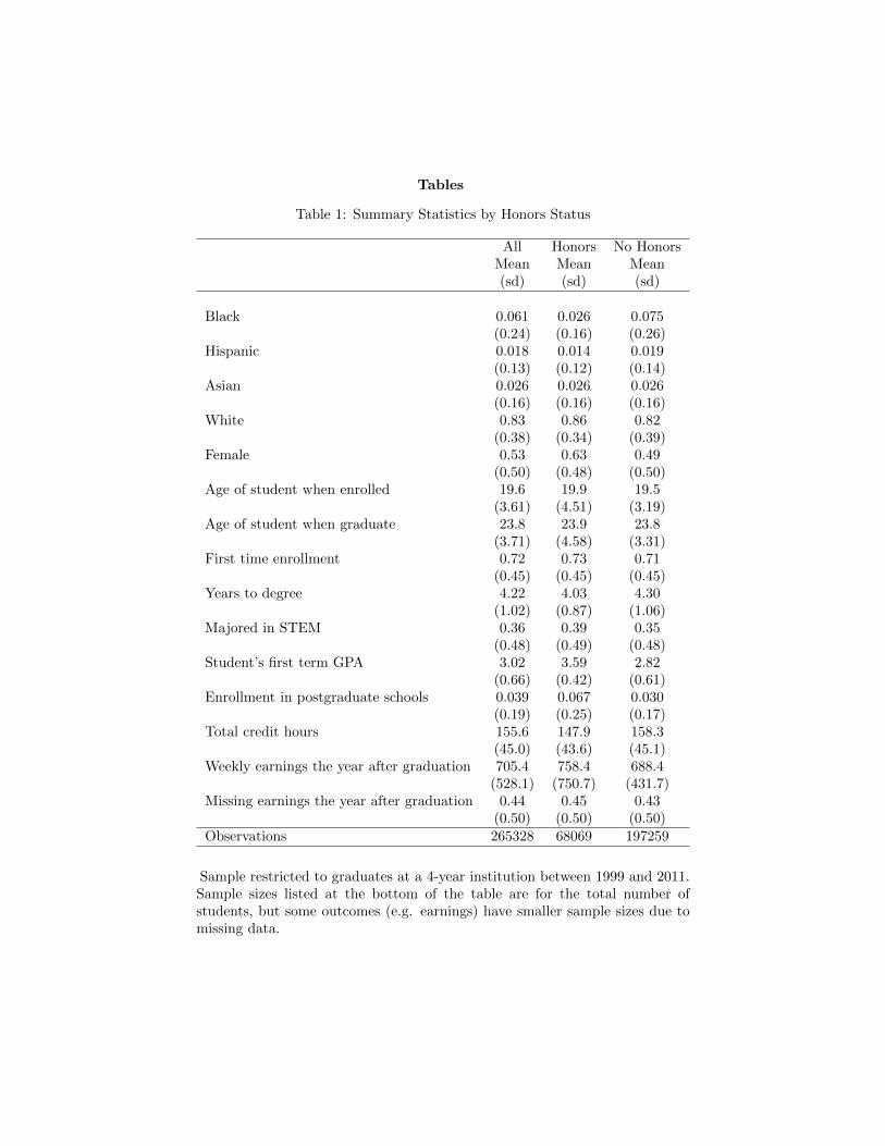
Table 1 shows basic descriptive statistics for the overall sample, the set of students who

obtain cum laude and the set of students who do not obtain cum laude. The cum laude column

includes students who obtain magna or summa cum laude. Table 1 shows that a large majority

of the state of Ohio is white and this is even more true among students who obtain honors.

Fewer than 2 percent of the sample are Hispanic and only 6 percent of the sample are black.

Students who obtain honors complete the degree in slightly less time than other students and

complete fewer credits. Not surprisingly, students who eventually obtain cum laude have

substantially higher first-term GPAs compared to other students.

The second to last row of Table 1 shows that students who obtain honors earn

approximately $70 more per week compared to students who do not obtain honors. This

difference could reflect the causal effect of honors on weekly earnings, but it could also reflect

observed and unobserved differences between those with honors and those without. The final

row of Table 1 shows that we observe no earnings for approximately 44 percent of college

graduates. This is similar to past work that uses UI data from a single state (Zimmerman 2014)

and raises the possibility for sample selection to bias estimates. We explore this issue in a later

section.

Empirical Approach

14

Our analysis uses a sharp regression discontinuity design based on the fact that those

above the threshold obtain honors whereas those below the threshold do not. To implement the

analysis, we first construct our running variable, !" as

!" = $%&" − )*+,--" (1)

where $%&"is student i’s graduating cumulative GPA and )*+,--" is the relevant cutoff for cum

laude honors based on student i’s college and major. Using this running variable, we then

estimate

." = /!" + 12" + 3!"2" + )*+,--"4 + 5" (2)

where ."denotes wages in the year following graduation, !" is the running variable defined

above and 2" is an indicator for whether !" is above zero or not. )*+,--" is a vector of indicator

variables controlling for the cutoff required to obtain cum laude. In some specifications, we

include additional student-level covariates, school fixed effects and year fixed effects. We

include cutoff fixed effects in all specifications to account for the fact that the composition of

students differs across different cutoffs. The results are almost identical if we instead include

institution fixed effects. Though in our context the running variable is virtually continuous, we

also cluster on the running variable based on the recommendation of Card and Lee (2008).

We implement the RD analysis following the various recommendations from Imbens and

Lemieux (2008). We begin the RD analysis by presenting all of our results in figure form. We

then estimate local-linear regression with the aim of matching the visual evidence from the

figures. For our preferred estimates, we use the IK optimal bandwidth described in Imbens and

Kalyanaraman (2011), but we also explore the robustness of our results to a variety of other

bandwidths. To assess the likelihood that differences in the characteristics of those just above

15

and just below the threshold lead to biased estimates, we show that results are very similar when

we control for covariates.

Specification Tests

A key concern is the possibility that students finely manipulate their GPA in order to land

just above the honors threshold. This is a serious concern in our context because thresholds are

publicly known, and students can theoretically alter their effort in order to obtain honors. That

said, whether students are able to finely manipulate their GPA in order to obtain honors is an

empirical question. Students may not view obtaining Latin honors to be sufficiently important to

justify substantially altering their effort or they may lack the ability to finely manipulate GPA.

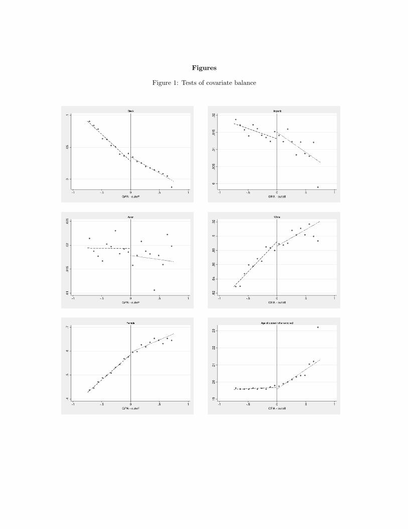
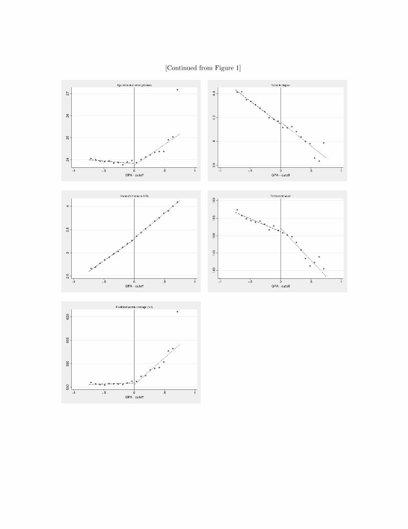
We are able to provide substantial empirical evidence on this question both by visually

inspecting the histogram of the running variable and by directly testing for whether there is

sorting correlated with observable characteristics.

The first 10 plots in Figure 1 investigate whether there are discontinuities in any of the

observable covariates at the threshold. Table 2 shows the RD estimates associated with each of

these plots. We use the IK optimal bandwidth for each outcome, which is why sample sizes vary

by outcome. Across all specifications, none show a statistically significant discontinuity—even

at the 10% level. We take these findings as suggesting that students do not manipulate GPA in a

way that is correlated with observable characteristics. It is worth emphasizing that many of the

covariates that we test are likely to be related to a variety of unobservables that one might be

concerned with.

As a summative way to investigate covariate imbalance, we use all of our covariates to

predict earnings in the year after graduation. We then examine whether there is a discontinuity

16

in predicted earnings at the honors threshold. The last row of Table 2 shows no evidence of a

discontinuity in predicted earnings. This suggests that based on their observable characteristics,

we have no reason to expect that those just above the honors threshold would earn more than

those just below the honors threshold.

Figure 2 shows the histogram of final GPAs, centered around the cum laude threshold. If

students who are just below the cum laude threshold manipulate their GPA to get just above the

cum laude threshold, we should observe a large valley just to the left of the threshold and a large

heap just to the right of the threshold. The figures shows no evidence of this pattern, providing

further reassurance that students do not finely manipulate the running variable in this context.

Results

Figure 3 presents our main results of the effect of cum laude on weekly earnings in the

year after graduation. Figure 3a shows the result for the overall sample, while Figure 3b and

Figure 3c split the sample by the selectivity of the school. Overall, Figure 3a shows evidence of

a discontinuity in earnings right at the threshold. Based on Figures 3b and 3c, it is clear that the

overall discontinuity is driven by a discontinuity among the selective schools and there is no

visual evidence of a discontinuity for non-selective schools.

Table 3 provides exact discontinuity estimates along with standard errors for the overall

sample and split by selectivity. In addition to showing our preferred estimates that use the IK

optimal bandwidth and include controls, Table 3 also shows robustness to a variety of bandwidth

choices, with and without controls. Before discussing the results, it is worth noting that the

stability of the estimates across bandwidth choices is reassuring that our preferred specification

17

reasonably captures the visual discontinuities shown in Figures 3a, 3b and 3c. Similarly, it is

reassuring that the estimates are relatively stable when covariates are added.

For the overall sample, we estimate that the discontinuity is approximately $25 per week

or roughly 3% of weekly wages. This estimate is statistically significant at the 10 % level in

most specifications. For the selective schools, the estimated discontinuity is larger in magnitude

and statistically significant at the 10 % level in most of the specifications. For non-selective

schools, none of the estimates are statistically significant and the sign of the estimated

discontinuity varies across bandwidth choices. The results presented in Table 3 confirm our

visual inspection of Figure 3, namely that there is a discontinuity in weekly earnings at the cum

laude threshold that is concentrated among students attending selective schools. We view the

statistical insignificance of the 0.25 bandwidth estimates as reflecting a lack of power as opposed

to suggesting that there is not a cum laude effect. In particular, the estimates are very similar

with the small bandwidth, simply with larger standard errors. Although it is important that our

point estimates are stable to bandwidth changes, the lack of statistical significance for the

smallest bandwidth does not strike us as problematic. In particular, statistical insignificance

means that an estimate is plausibly explainable by sampling variation, and the general pattern of

results shown in Figure 3 and Table 3 suggest that the cum laude effect is not driven by sampling

variation.

In Figures 4a-4c, we show the estimated effect of cum laude honors on earnings 2 years

after college. Figures 4a-4c show a similar pattern to the earlier results, where there is a visually

apparent earnings discontinuity at the cum laude threshold, and this effect is driven entirely by

students from selective schools. Table 4 shows the exact point estimates along with standard

errors. In terms of the point estimates, earnings in the second year after college are affected by

18

cum laude very similarly to earnings immediately after college. The point estimates are

somewhat larger, but they are also considerably noisier so that none of the specifications are

statistically significant. Given this noisiness, the estimates shown in Table 4 are statistically

indistinguishable from the estimates from Table 3.

In Figures 5a-5c, we show the estimated effect of cum laude honors on earnings 3 years

after college. These figures show a very different pattern compared to the earlier results as there

is no evidence of earnings discontinuities for any of the samples. Table 5 shows the exact point

estimates along with standard errors. Earnings in the third year after college appears to be

unrelated to cum laude. None of the specifications are statistically significant and the point

estimates vary in sign across bandwidth choices. Combined with the earlier results, we interpret

this finding as suggesting that Latin honors provides employers of recent graduates with a

valuable signal, but after several years, employers do not rely on this signal because they have

access to more directly relevant information such as work experience and job performance.

Based on this theory, we expected that the year two earnings estimates would be smaller than the

year one earnings estimates, but we did not see this pattern. Although we have no explanation

for why there is no decline in the premium across the first two years, it is worth noting that the

large standard errors of the second-year estimates prevent us from concluding that the premium

did not decline across years. In particular, the 90% confidence interval for the second-year

earnings effect includes many estimates that would be consistent with a declining premium.

Because we are only able to observe earnings for individuals who remain in Ohio after

graduation, our estimates have the potential to be biased by differential sample attrition.

Specifically, if cum laude causes the very best (or worst) to leave the state, this will lead to

biased estimates, even if there is no running variable manipulation. To investigate the likelihood

19

that sample attrition biases our estimates, we estimate whether there is a discontinuity in the

probability of missing earnings information at the cum laude threshold. Because sample attrition

increases the further we look after college, we test for the possibility of differential attrition one,

two and three years after graduating.

Table 6 shows our estimates of the discontinuity in missing earnings in the year after

graduation. Figures 6a-6c show the corresponding figures. Table 6 shows that the estimated

discontinuities are all small in magnitude and switch signs across specifications. None of the

estimates are statistically significant. It is important to note that even if the estimates in Table 6

were all statistically significant, the magnitude is much too small to generate substantial bias

since at most, the point estimates imply less than 1% differential attrition.

Table 7 and Table 8 examine whether there is differential attrition in the second or third

year following graduation. Figures 7a-7c and 8a-8c show the corresponding figures. As with

the first-year attrition results, we see very little evidence of differential attrition with all of the

estimates quite small and only one statistically significant at the 10% levels. The results shown

in the tables confirm our visual inspection of Figures 7 and 8, which suggest no discontinuities in

the probability of missing earnings.

Conclusion

We provide the first estimates of the effect of Latin honors on earnings. Our estimates

are based on a regression discontinuity design that helps us to distinguish the Latin honors effect

from unobserved differences between students who obtain honors and those who do not. We

find that Latin honors increases earnings in the year immediately after college graduation, but the

20

earnings benefit does not persist. Students at non-selective colleges do not derive an earnings

benefit from obtaining Latin honors.

While we have no definitive explanation for the difference between selective and non-

selective schools, there are many possible explanations. First, Robst (1995) notes that graduates

of non-selective colleges often compete for jobs with non-graduates and are generally much

more likely to be employed in a job that does not require a college degree. It is possible that the

distinction between having college degree vs not having a college degree dominates

considerations such as the academic performance of the college graduate. Second, it is possible

that employers who hire non-selective college graduates place a lower value on academic

success. Third, it is possible that employers perceive non-selective college coursework as less

rigorous and therefore discount high grades from such institutions. The above explanations are

not exhaustive since a lack of a signaling effect at non-selective schools could be explained by a

variety of other factors.

Although our study is focused on the effect of Latin honors, it relates to the literature

studying whether employers value academic performance more generally. Many studies have

shown that there is a positive correlation between college GPA and earnings, but all of these

studies face the major obstacle that college GPA is correlated with a variety of unobservables

that are likely to directly affect earnings. Employers may value GPA either because they view

academic performance as directly productive, or because academic performance is correlated

with productive factors that the firm cannot observe. In either case, GPA would have a causal

effect on earnings. Past research on the relationship between GPA and earnings, however, could

be driven by a non-causal relationship between academic performance and earnings if there are

characteristics that are observable to the employer, but unobservable to the econometrician. We

21

are not aware of evidence that demonstrates that there is a causal relationship between academic

performance and earnings in the United States. Our findings suggest that employers value

academic performance among students at selective colleges. Naturally, our lack of an effect at

non-selective colleges does not imply that employers do not value other measures of academic

success at these schools.

A few caveats are worth emphasizing regarding our results. First, the regression

discontinuity design estimates the benefit of Latin honors for students at the margin. Because we

are focused on the cum laude threshold (as opposed to the summa or magna cum laude

thresholds) our estimates apply to strong students, but not the very best. For our sample, this

corresponds to roughly the 75th percentile of graduates. It is possible that the top or bottom of

the distribution would derive a larger or smaller benefit from Latin honors. Second, our estimates

are based on the subset of students who remain in the state of Ohio and are not self-employed.

We show that there is no differential attrition in terms of missing wages suggesting that we are

able to credibly identify the wage effects among the set of students who are not missing earnings.

In terms of external validity, however, it is important to keep in mind that our estimates may not

apply to students who leave the state of Ohio or are self-employed.

Designating certain students as cum laude is a nearly costless policy that has the potential

to help employers distinguish between candidates. For a college administrator deciding where to

set the threshold, there are several factors to consider. Reducing the threshold necessary to

obtain Latin honors provides the benefit of the signal to more students, but it has the potential to

dilute, and perhaps destroy the signaling value of the designation. Our study provides evidence

on the ceteris paribus effect of obtaining cum laude and does not incorporate this general

equilibrium effect. Thus, our estimates should be taken as the effect of cum laude for an

22

individual student, as opposed to indicative of the likely effect if institutions alter their

thresholds.

23

Works Cited Arcidiacono, P., Bayer, P., & Hizmo, A. (2010). Beyond Signaling and Human Capital:

Education and the Revelation of Abilit. American Economic Journal: Applied Economics, 2(4), 76-104.

Chan, H. F., Frey, B. S., Gallus, J., & Torgler, B. (2014). Academic honors and

performance. Labour Economics, 31, 188-204.

Clark, D., & Martorell, P. (2014). The signaling value of a high school diploma. Journal

of Political Economy, 122(2), 282-318.

Feng, A., & Graetz, G. (2013). A question of degree: the effects of degree class on labor market

outcomes. Unpublished manuscript. Flores-Lagunes A. & Light A. (2010) Interpreting Degree Effects in the Returns to Education.

Journal of Human Resources, Vol (45) No. 2 pp. 439-467. Freier, R., Schumann, M., & Siedler, T. (2015). The earnings returns to graduating with

honors—Evidence from law graduates. Labour Economics, 34, 39-50. Hungerford, T., & Solon, G. (1987). Sheepskin effects in the returns to education. The review of

economics and statistics, 175-177. Imbens, G., & Kalyanaraman, K. (2011). Optimal bandwidth choice for the regression

discontinuity estimator. The Review of Economic Studies. Imbens, G. W., & Lemieux, T. (2008). Regression discontinuity designs: A guide to practice.

Journal of econometrics, 142(2), 615-635. Jaeger D. A. & Page M. E. (1996) New Evidence on Sheepskin Effects and the Returns to

Education. Review of Economics and Statistics,Vol (78) No. 4 pp. 733-740. Kane T. J. & Rouse C. E. (1995) Labor-Market Returns to Two- and Four-Year College.

American Economic Review, Vol (85) No. 3 pp. 600-614. Lee, D. S., & Card, D. (2008). Regression discontinuity inference with specification error.

Journal of Econometrics, 142(2), 655-674. Neckermann, S., Cueni, R., & Frey, B. S. (2014). Awards at work. Labour Economics, 31, 205-

217. Nederhof, A., & Van Raan, A. (1987). Peer review and bibliometric indicators of scientific

performance: a comparison of cum laude doctorates with ordinary doctorates in physics. Scientometrics, 11(5-6), 333-350.

24

Robst, J. (1995). College quality and overeducation. Economics of Education Review, 14(3), 221-228.

Spence, M. (1973). Job market signaling. The Quarterly Journal of Economics, 355-374. Svrluga, Susan. "More than 4 out of 5 Students Graduate without a Job. How Could Colleges

Change That?" Washington Post. The Washington Post, 30 Jan. 2015. Web. 21 Nov. 2016.

Takalkar, P. (1993). A Search for Truth in Student Responses to Selected Survey Items. AIR

1993 Annual Forum Paper. Tyler, J. H., Murnane, R. J., & Willett, J. B. (2000). Estimating the labor market signaling

value of the GED. Quarterly Journal of Economics, 431-468.

Zimmerman, S. D. (2014). The returns to college admission for academically marginal students.

Journal of Labor Economics, 32(4), 711-754.

Tables

Table 1: Summary Statistics by Honors Status

All Honors No HonorsMean Mean Mean(sd) (sd) (sd)

Black 0.061 0.026 0.075(0.24) (0.16) (0.26)

Hispanic 0.018 0.014 0.019(0.13) (0.12) (0.14)

Asian 0.026 0.026 0.026(0.16) (0.16) (0.16)

White 0.83 0.86 0.82(0.38) (0.34) (0.39)

Female 0.53 0.63 0.49(0.50) (0.48) (0.50)

Age of student when enrolled 19.6 19.9 19.5(3.61) (4.51) (3.19)

Age of student when graduate 23.8 23.9 23.8(3.71) (4.58) (3.31)

First time enrollment 0.72 0.73 0.71(0.45) (0.45) (0.45)

Years to degree 4.22 4.03 4.30(1.02) (0.87) (1.06)

Majored in STEM 0.36 0.39 0.35(0.48) (0.49) (0.48)

Student’s first term GPA 3.02 3.59 2.82(0.66) (0.42) (0.61)

Enrollment in postgraduate schools 0.039 0.067 0.030(0.19) (0.25) (0.17)

Total credit hours 155.6 147.9 158.3(45.0) (43.6) (45.1)

Weekly earnings the year after graduation 705.4 758.4 688.4(528.1) (750.7) (431.7)

Missing earnings the year after graduation 0.44 0.45 0.43(0.50) (0.50) (0.50)

Observations 265328 68069 197259

Sample restricted to graduates at a 4-year institution between 1999 and 2011.Sample sizes listed at the bottom of the table are for the total number ofstudents, but some outcomes (e.g. earnings) have smaller sample sizes due tomissing data.

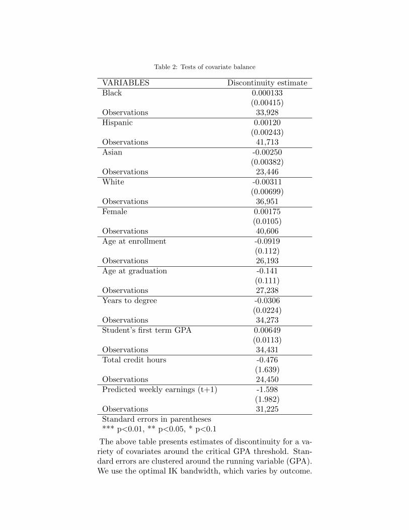
Table 2: Tests of covariate balance

VARIABLES Discontinuity estimateBlack 0.000133

(0.00415)Observations 33,928Hispanic 0.00120

(0.00243)Observations 41,713Asian -0.00250

(0.00382)Observations 23,446White -0.00311

(0.00699)Observations 36,951Female 0.00175

(0.0105)Observations 40,606Age at enrollment -0.0919

(0.112)Observations 26,193Age at graduation -0.141

(0.111)Observations 27,238Years to degree -0.0306

(0.0224)Observations 34,273Student’s first term GPA 0.00649

(0.0113)Observations 34,431Total credit hours -0.476

(1.639)Observations 24,450Predicted weekly earnings (t+1) -1.598

(1.982)Observations 31,225Standard errors in parentheses*** p<0.01, ** p<0.05, * p<0.1

The above table presents estimates of discontinuity for a va-riety of covariates around the critical GPA threshold. Stan-dard errors are clustered around the running variable (GPA).We use the optimal IK bandwidth, which varies by outcome.

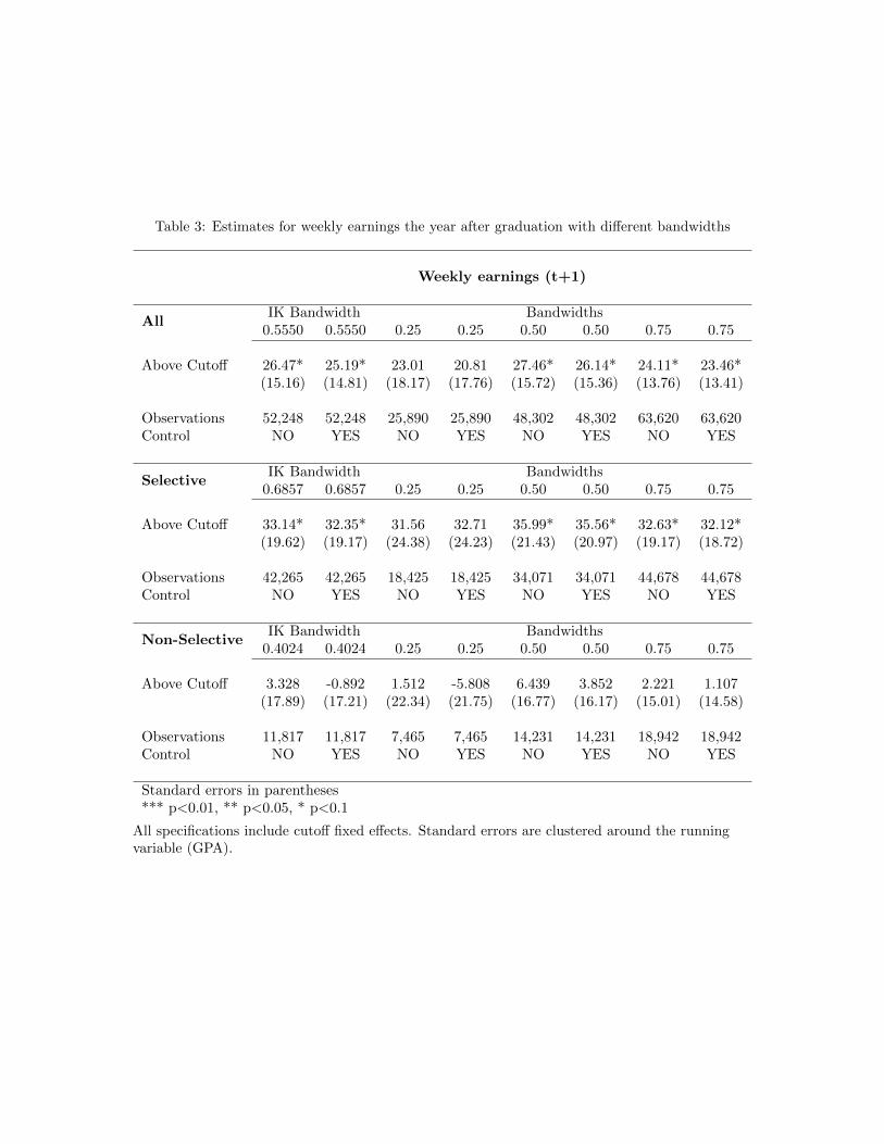
Table 3: Estimates for weekly earnings the year after graduation with di↵erent bandwidths

Weekly earnings (t+1)

All

IK Bandwidth Bandwidths0.5550 0.5550 0.25 0.25 0.50 0.50 0.75 0.75

Above Cuto↵ 26.47* 25.19* 23.01 20.81 27.46* 26.14* 24.11* 23.46*(15.16) (14.81) (18.17) (17.76) (15.72) (15.36) (13.76) (13.41)

Observations 52,248 52,248 25,890 25,890 48,302 48,302 63,620 63,620Control NO YES NO YES NO YES NO YES

Selective


Above Cuto↵ 33.14* 32.35* 31.56 32.71 35.99* 35.56* 32.63* 32.12*(19.62) (19.17) (24.38) (24.23) (21.43) (20.97) (19.17) (18.72)


Non-Selective


Above Cuto↵ 3.328 -0.892 1.512 -5.808 6.439 3.852 2.221 1.107(17.89) (17.21) (22.34) (21.75) (16.77) (16.17) (15.01) (14.58)


Standard errors in parentheses*** p<0.01, ** p<0.05, * p<0.1

All specifications include cuto↵ fixed e↵ects. Standard errors are clustered around the runningvariable (GPA).

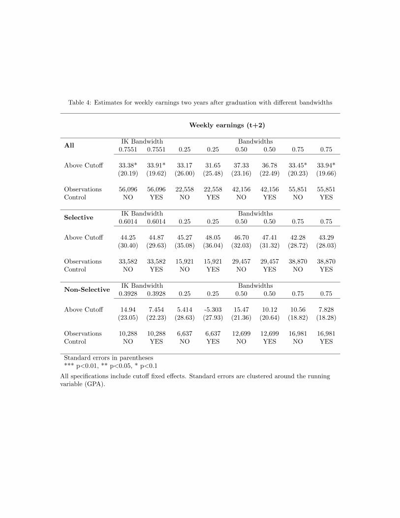
Table 4: Estimates for weekly earnings two years after graduation with di↵erent bandwidths


All


Above Cuto↵ 33.38* 33.91* 33.17 31.65 37.33 36.78 33.45* 33.94*(20.19) (19.62) (26.00) (25.48) (23.16) (22.49) (20.23) (19.66)


Selective


Above Cuto↵ 44.25 44.87 45.27 48.05 46.70 47.41 42.28 43.29(30.40) (29.63) (35.08) (36.04) (32.03) (31.32) (28.72) (28.03)


Non-Selective


Above Cuto↵ 14.94 7.454 5.414 -5.303 15.47 10.12 10.56 7.828(23.05) (22.23) (28.63) (27.93) (21.36) (20.64) (18.82) (18.28)




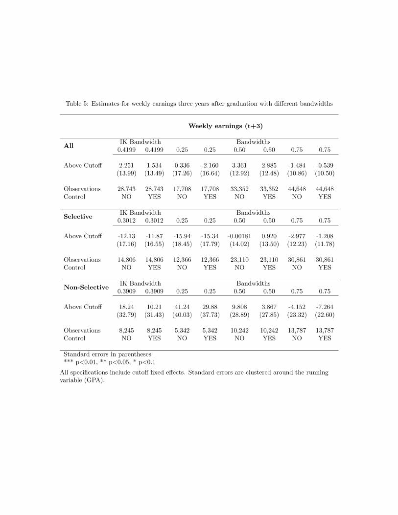
Table 5: Estimates for weekly earnings three years after graduation with di↵erent bandwidths


All


Above Cuto↵ 2.251 1.534 0.336 -2.160 3.361 2.885 -1.484 -0.539(13.99) (13.49) (17.26) (16.64) (12.92) (12.48) (10.86) (10.50)


Selective


Above Cuto↵ -12.13 -11.87 -15.94 -15.34 -0.00181 0.920 -2.977 -1.208(17.16) (16.55) (18.45) (17.79) (14.02) (13.50) (12.23) (11.78)


Non-Selective


Above Cuto↵ 18.24 10.21 41.24 29.88 9.808 3.867 -4.152 -7.264(32.79) (31.43) (40.03) (37.73) (28.89) (27.85) (23.32) (22.60)




Table 6: Estimates for missing earnings the year after graduation with di↵erent bandwidths

Missing earnings (t+1)

All


Above Cuto↵ -0.000132 0.000537 -0.00139 0.00322 -1.57e-05 0.000419 -0.000932 -0.000585(0.00518) (0.00450) (0.00714) (0.00618) (0.00508) (0.00442) (0.00436) (0.00378)


Selective


Above Cuto↵ 0.00127 0.00187 0.00183 0.00422 0.00128 0.00127 -0.000329 4.61e-05(0.00659) (0.00584) (0.00823) (0.00728) (0.00594) (0.00526) (0.00517) (0.00458)


Non-Selective


Above Cuto↵ -0.00627 -0.00247 -0.0115 0.00129 -0.00478 -0.00310 -0.00371 -0.00497(0.0102) (0.00847) (0.0134) (0.0112) (0.00949) (0.00789) (0.00801) (0.00661)




Table 7: Estimates for missing earnings two years after graduation with di↵erent bandwidths


All


Above Cuto↵ 0.00630 0.00777 0.00922 0.0112* 0.00347 0.00352 0.000853 0.000830(0.00625) (0.00573) (0.00719) (0.00656) (0.00508) (0.00470) (0.00437) (0.00403)


Selective


Above Cuto↵ 0.00475 0.00523 0.00762 0.00858 0.00181 0.00125 -0.000693 -0.00116(0.00711) (0.00669) (0.00807) (0.00758) (0.00584) (0.00552) (0.00511) (0.00482)


Non-Selective


Above Cuto↵ 0.00979 0.0140 0.0132 0.0192 0.00671 0.00857 0.00258 0.00267(0.0116) (0.0106) (0.0141) (0.0129) (0.00980) (0.00892) (0.00820) (0.00744)




Table 8: Estimates for missing earnings three years after graduation with di↵erent bandwidths


All


Above Cuto↵ 0.00233 0.00267 0.00418 0.00551 0.00120 -0.000182 -8.60e-05 -0.00203(0.00609) (0.00572) (0.00678) (0.00637) (0.00490) (0.00460) (0.00422) (0.00395)


Selective


Above Cuto↵ 0.00508 0.00457 0.00647 0.00663 0.00293 0.000197 0.00208 -0.00193(0.00748) (0.00718) (0.00802) (0.00772) (0.00579) (0.00554) (0.00506) (0.00481)


Non-Selective


Above Cuto↵ -0.00368 -0.000745 -0.00244 0.00270 -0.00454 -0.00155 -0.00688 -0.00288(0.0114) (0.0104) (0.0137) (0.0125) (0.00966) (0.00879) (0.00812) (0.00737)




Figures

Figure 1: Tests of covariate balance

[Continued from Figure 1]

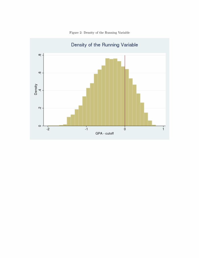
Figure 2: Density of the Running Variable

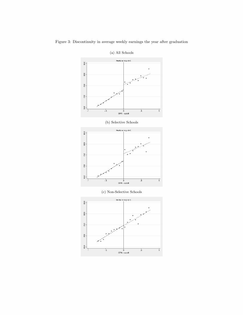
Figure 3: Discontinuity in average weekly earnings the year after graduation

(a) All Schools

(b) Selective Schools

(c) Non-Selective Schools

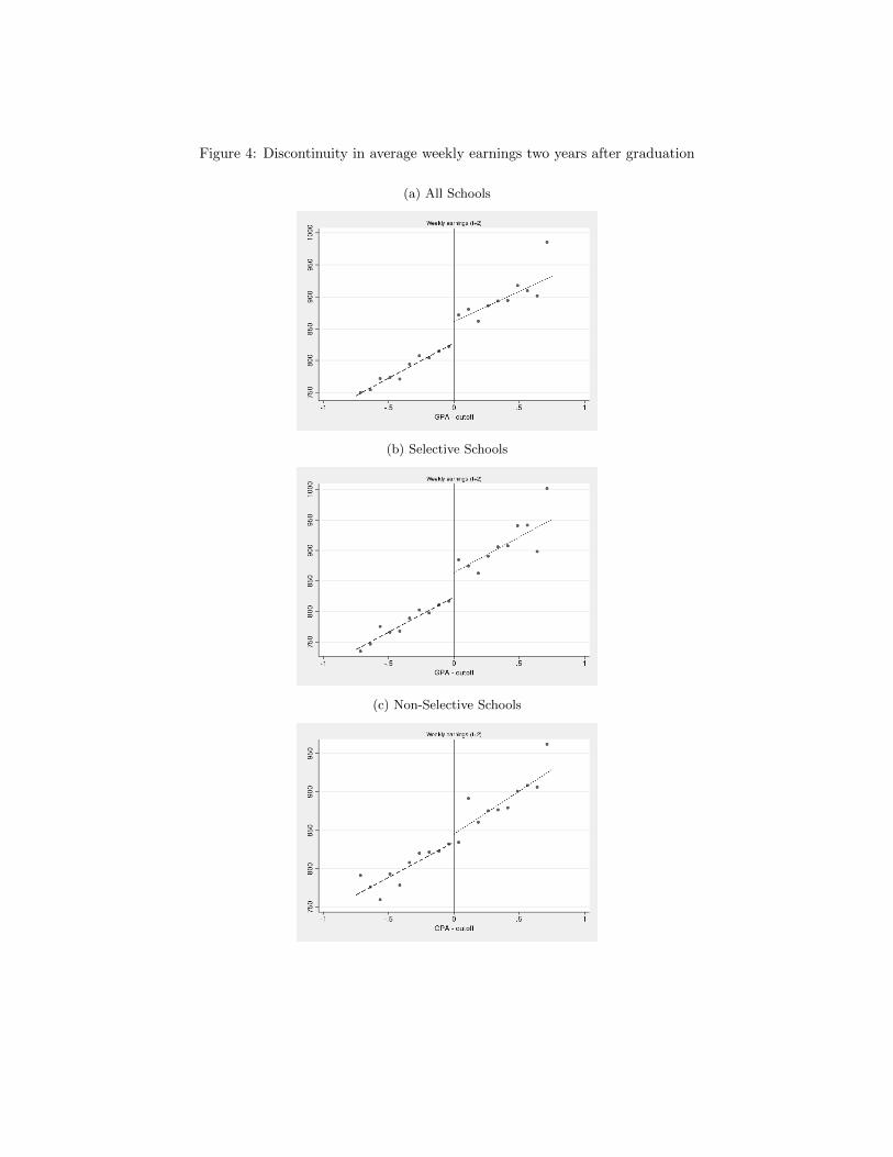
Figure 4: Discontinuity in average weekly earnings two years after graduation

(a) All Schools



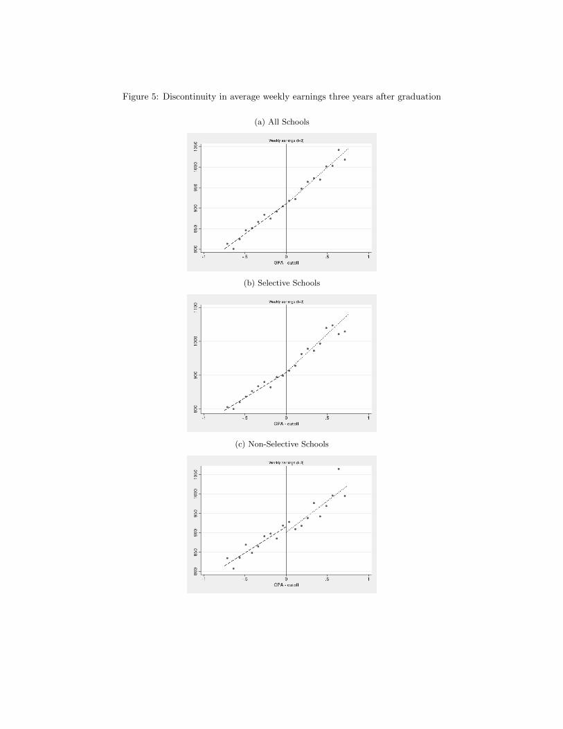
Figure 5: Discontinuity in average weekly earnings three years after graduation

(a) All Schools



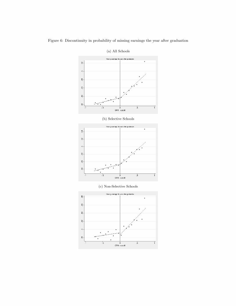
Figure 6: Discontinuity in probability of missing earnings the year after graduation

(a) All Schools



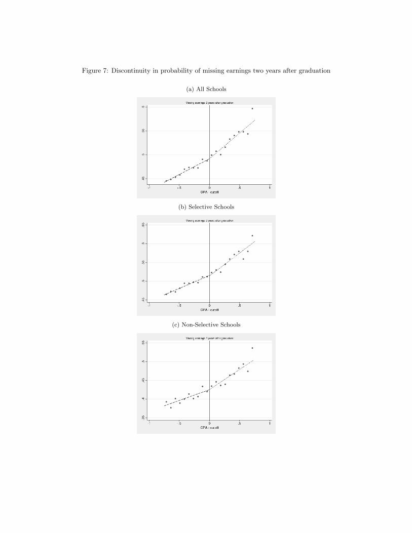
Figure 7: Discontinuity in probability of missing earnings two years after graduation

(a) All Schools



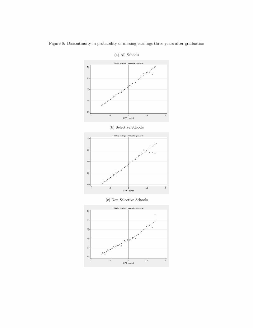
Figure 8: Discontinuity in probability of missing earnings three years after graduation

(a) All Schools



Documents

The Effect of Latin Honors on Earnings