The Effect of Identity Preserved Premiums on Elevator ...ageconsearch.umn.edu/bitstream/21955/1/sp03gl01.pdf · The effect of identity preserved premiums on a grain ... of Identity

1

The Effect of Identity Preserved Premiums on Elevator Grain Flows

Angela Gloy and Frank Dooley Department of Agricultural Economics

Purdue University

Abstract: The effect of identity preserved premiums on a grain elevator’s received volumes is modeled using stochastic simulation across the harvest season. A feedback loop simulates competing elevators’ bid prices and tracks producer delivery decisions using arbitrage criteria at competing market elevators. Results provide information about the sensitivity of distance thresholds in producer delivery decisions given IP premiums. Keywords: Identity preserved, market areas, arbitrage

Selected Paper at the American Agricultural Economics Association Annual Meeting

July 27-30, 2002, Montreal

Copyright 2003 by Angela Gloy and Frank Dooley. All rights reserved. Readers may make verbatim copies of this document for non-commercial purposes by any means, provided that this copyright notice appears on all such copies.

Frank Dooley

Department of Agricultural Economics Purdue University

West Lafayette, IN 47907-1145 [email protected]

2

The Effect of Identity Preserved Premiums on Elevator Grain Flows

For any given grain elevator, information flows among producers, end users, and

competitor grain elevators. These three categories of market participants generate market-level

information that is used internally to maximize the profitability of a particular elevator.

In large part, producer-generated information revolves around total grain volume, as well

as the types and quality characteristics of grains produced. Annual production forecasts, based

on historical trend, provide elevators with estimates of grains available to be supplied to an

elevator. Often greater uncertainty surrounds not the total volumes produced, but rather the

distribution of grain types and qualities. In addition, the elevator is concerned with the

producer’s transport costs. The combination of three factors, distance to elevator, elevator bid

price, and producer transport costs per mile, determine which elevator receives the producer’s

grain. Or, the possibility exists that the elevator is by-passed altogether in the case of direct

producer to end-user shipment. In short, factors influencing arbitrage conditions are critical

pieces of producer-generated information used by elevator management.

With respect to end users, the three most likely outlets for corn and soybean usage from

the Eastern Corn Belt are food processors (such as crushing mills, wet or dry corn milling, etc.),

feed lots, or barge facilities in preparation for export. Historical trends provide reasonable

estimates for grain usage by type of user. Food processors and feedlots have exhibited fairly

consistent demand patterns over time with greater variation seen in the volumes demanded in

export markets.

A commodity-based grain marketing environment invites cost minimization because of

high-volume, low-margin product characteristics. Commodity-intensive markets encourage

3

elevator managers to attract the largest grain volumes possible, subject to facility configuration

constraints, at the lowest possible per unit cost. Attracting grain flows to an elevator is a function

of arbitrage conditions, in turn highlighting the bid price-producer distance relationship.

Because commodities do not draw over cash price premia, the producer’s shipping cost to an

elevator is the determining factor in their delivery decision.

The variable premium structure associated with identity preserved (IP) grains, however,

implies a shift in the weight, or value, that bid prices and producer distances carry relative to one

another, as producers evaluate their best delivery option. Per bushel IP premiums offered at a

mid-range distance elevator could offset the higher transportation cost of delivery compared to

those of a closer elevator not offering the same premium. More specifically, IP premiums

influence the market boundaries at which elevators compete for producer deliveries. Thus, an

elevator’s competitive strategy should incorporate information about competitor elevators’ bid

prices. Assuming competing elevators are angling for the same grain types in a market area, a

better understanding of a competitor’s bid price distribution might translate into a competitive

pricing strategy advantage.

The objective of this paper is to evaluate the effect of competitor bid price offerings on a

case study elevator’s grain flows during the harvest season. This paper is an effort to better

understand the extent to which grain flows are altered with incremental changes and variation in

the closest competitors’ marketing margin. Particular emphasis is placed on examination of

arbitrage conditions in so far as they drive producer delivery decisions.

The intent of this paper is to build on one part of Maltsbarger’s IP-opportunity cost

argument using stochastic market feedback. In particular, grain volumes lost to competitors is

lost revenue, if an elevator could have received, handled, and stored the same grain without

4

compromising operational efficiency. Operational efficiency is further complicated by IP grains

through attribute preservation assurance. The results of this study play a role in evaluating the

economic impacts of IP grain production at the elevator level. The grain flows examined in this

study can be used with cost estimates and blending models to determine the total economic

impact on a given elevator’s profitability. However, a thorough understanding of the

competitive situation and grain flows are a necessary first step to understanding this problem.

The paper is divided into 5 sections. First, previous studies are reviewed for their

contribution to this discussion of market area definition, assembly costs, and arbitrage

conditions. The second section discusses the methodology. Third, the paper outlines model

details including scenario and variable specification, as well as model assumptions. Scenario

results are presented in section four. The paper concludes with an interpretation of broader,

market consequences implied by the results and suggests future extensions of this research.

Literature Review

Three themes in the literature are reviewed. First, spatial price differentials are examined

as a function of micro-market structure. Second, the role of producer assembly costs is

addressed as it influences elevator manager’s perception of total facility costs. Third, a review of

arbitrage conditions follows to the extent that they influence a grain elevator’s market definition.

The degree to which micro-market structure explains spatial grain price differentials is

motivated by observation that price differentials exist which cannot be attributed to time, space,

and form cost variables (Jones; Davis and Hill; McCully). Market variables related to elevator

scale and scope, elevator transport options, and proximity to competitors are used to capture

market structure effects. The breadth of marketing services offered by an elevator, as well as

5

competitor density emerge as salient factors influencing elevator bid prices (Jones, Davis and

Hill; Wenzel et al.).

Wenzel et al. identify three factors contributing to an elevator’s ability to offer alternative

bid prices: (1) local supply and demand conditions, (2) firm productive efficiency, and (3)

operating practices. This research addresses two of these factors. First, local demand and supply

conditions are fixed in any given grain marketing year thereby making elevator managers in a

given market area compete for a fixed volume in the short run. Second, this research draws

attention to the efficiency-volume/type trade-off. Identity preservation likely hinders operational

efficiency, relative to the commodity-only scenario. Because an elevator offers higher IP

premiums compared to their competitors does not imply they have achieved greater operational

efficiency. One of the challenges for elevator managers is to identify how to most effectively

adjust bid prices without compromising operational efficiency. This research highlights the

inter-relatedness of Wenzel et al.’s second and third market factors, namely operational

efficiency and operating practices.

Operational efficiency connotes maximum output at the lowest possible cost, subject to

technological/production constraints. Misreading costs can hinder achieving operational

efficiency. Araji and Walsh (1969) find that inclusion of previously omitted assembly costs

significantly impacts the elevator’s cost curves.1 Previous studies maintained that storage,

handling, and loading grains processes provided a complete cost summary. Under this

assumption, indirect (marketing) costs are overlooked.

In a commodity only environment, average costs are non-increasing as economies of

scale are recognized. The average total costs should also stabilize with larger throughput

1 Assembly cost factors are defined here as “grain sales density and the costs of hauling grain from farm to elevator” (Araji and Walsh, 36).

6

volumes. Araji and Walsh argue, however, that exclusion of assembly costs guides managers to

expand facility size beyond what is the true profit maximizing capacity. That is, assembly costs,

which are a function of grain sales density and producer transport costs, increase with distance.

Managers basing their decisions on market area volume need also consider producer-elevator

distances in determining which facility receives the grain. Producers traveling greater distances

incur greater assembly costs, assuming a constant per mile truck cost. At some distance though,

producers will deliver to another facility. In this respect, assembly costs are a type of

opportunity cost. Managers who pursue increased storage capacity without considering

assembly costs will overestimate their optimal size, by misunderstanding market boundaries.

Inclusion of a feedback mechanism draws attention to arbitrage conditions. Elevators in

any given market are assumed to be price takers and thus all confront the same terminal cash

market price (Dooley and Wilson). Factors then affecting arbitrage conditions include

producers’ assembly/transportation costs and elevator pricing strategies (Dooley and Wilson), or

where j = elevator competing with case study elevator i, P = price paid to producer by elevator i or j t = linear transportation cost incurred by producer for elevator delivery, and d = distance, in miles, from farm to elevator i or j.

Equation 1 offers a firm-level approach to examining competitive forces in a grain

market, in addition to making allowances for multiple facilities per market (Dooley and Wilson).

Using equation 1, producers compare delivery profit margins across all facilities, choosing the

one with the highest return for them. Three assumptions parameterize the model. First, it is

assumed that producers deliver to the elevator offering the highest price net of transportation

costs. Second, it is assumed that producers face uniform linear transport/assembly costs across

the market area. Finally, there is no allowance for price discrimination by elevators to producers.

jitdPtdP iijj ≠−=− ,)1(

7

Findings suggest that elevators raise their bid prices to offset competitors’ lower margins.

For example, if an elevator expands their transport capabilities to include multi-car rail

shipments, it effectively lowers their transport costs. These “savings” are then passed along to

producers in the form of higher bid prices. The smaller, single-car elevator’s (defensive)

response is to match the higher bid price so as to retain market share. These findings suggest

two points. First, the terminal price by itself is relevant only insofar as it affects elevators’

market spreads. For example, if the cash price increases by $0.05 but all elevators change their

bid prices by the same amount, the terminal price had no impact on the arbitrage conditions.

Second, elevator managers are limited in their ability to use bid prices as a means of market

boundary expansion due to the impact of producer transport costs.

Methodology

This analysis focuses on the impacts changes in arbitrage conditions have on a case study

elevator’s grain flows. Changes in a competitor’s marketing margins are viewed as being

derived from managerial decisions regarding asset configuration or pricing strategies. Grain

flows are directed toward or away from the case study elevator, depending on competitors’ bid

prices. The premise is that, within a given market, slight changes in elevator bid prices are

capable of drawing grain away from one facility to another.

A schematic of the model flow is provided in Figure 1. The model begins assuming that

grain producers stand ready to deliver harvest season grain. The first flow in Figure 1 is

informational – price signals are sent by elevators, and interpreted by producers (represented by

solid lines). Producers then evaluate all market arbitrage opportunities using equation 1 as their

guide. Producers will choose to deliver their grain to the facility whose bid price offers the

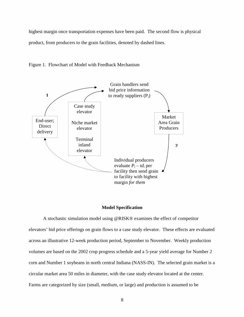
8

highest margin once transportation expenses have been paid. The second flow is physical

product, from producers to the grain facilities, denoted by dashed lines.

Figure 1. Flowchart of Model with Feedback Mechanism

Model Specification

A stochastic simulation model using @RISK® examines the effect of competitor

elevators’ bid price offerings on grain flows to a case study elevator. These effects are evaluated

across an illustrative 12-week production period, September to November. Weekly production

volumes are based on the 2002 crop progress schedule and a 5-year yield average for Number 2

corn and Number 1 soybeans in north central Indiana (NASS-IN). The selected grain market is a

circular market area 50 miles in diameter, with the case study elevator located at the center.

Farms are categorized by size (small, medium, or large) and production is assumed to be

Case study elevator

Niche market

elevator

Terminal inland

elevator

Grain handlers send bid price information to ready suppliers (Pi)

Individual producers evaluate Pi – tdi per facility then send grain to facility with highest margin for them

Market Area Grain Producers

End-user; Direct

delivery

1

2

9

distributed evenly across the market area. Three of the 4 competing elevators are located within

15 miles of the case study elevator. The fourth elevator is assumed to be located just inside the

market boundary.

Each week, equation 1 allocates available grain flows to all grain elevators in a given

market area. Each producer in the market is assumed to deliver to the facility offering the

highest return, net of transportation costs.

Changes to asset configuration may lower operational costs that can then be passed on to

producers in terms of higher bid prices. It is also possible that changes to asset configuration

could raise operational costs. Management’s involvement in pricing wars may lead to changes in

bid offerings to producers. Again, the priority is the case study elevator’s competitive response

to other market participants, not so much the derivation or impetus of a competitor’s move.

Changes in competitor IP premiums are interpreted relative to a baseline scenario absent

of price premiums. That is, grain flows are modeled using the market prices for all grain types

with no additional premium being offered by competing elevators. Scenario 2-4 adds a $0.02

over price premium to competitors 1, 2, and the case study elevator sequentially. A final

scenario evaluates the impact of offered premium variability, as the standard deviation in

competitor 2’s IP price distribution is reduced. Identity preserved grain price distributions are

the same across IP grain types per competitor.

Data

Construction of market area, producer, and grain facility profiles draws largely on data

provided by managers at the case study elevator and from Indiana Agricultural Select Indiana

counties are the building blocks of the given market area. Producer profiles are based on three

10

pieces of information: (1) producer density in the market area, (2) production volumes by farm

size, of acreage harvested, and (3) geographic location. Competitor elevator data, specifically

geographic location and bid price offerings, is defined relative to a case study elevator’s location

and historical cash price series.

The market area is defined as a six county region consisting of the five counties adjacent

to the case study elevator, plus the county in which the case study elevator is located. These

counties consistently appear in the state’s top 10 corn and soybean rankings for total production

and yield per acre in Indiana (IN NASS). In the six county market area, small farms (200-499

acres) account for 43 percent, or 610 of the total 1,405 farms (Table 1). Mid-size farms (500-999

acres) and large (1000+ acres) farms, account for 32 percent (454 farms) and 24 percent (341

farms) respectively (IN-NASS).

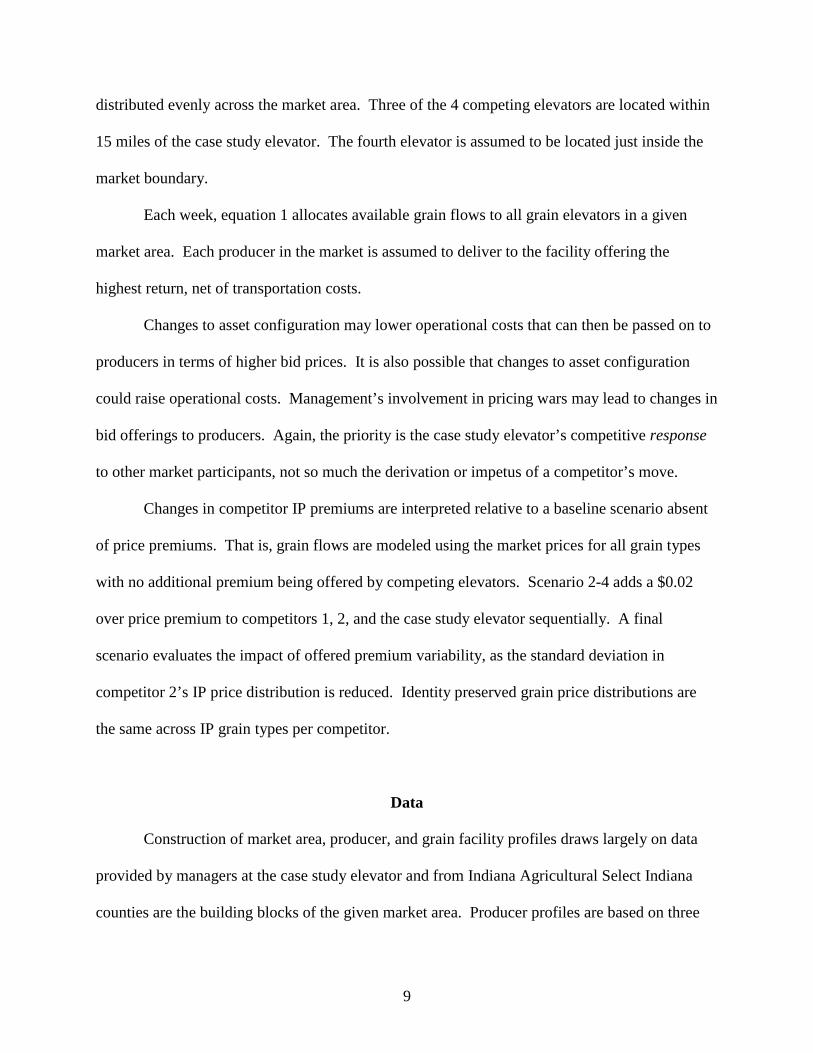
Table 1. Illustrative Farm Production Profile Farm Size (Acres) Average Harvested Acreage per Farm

200-499 326 500-999 701 1000+ 1,599

Source United States Department of Agriculture, Indiana Agricultural Statistics Service, http://www.nass.usda.gov/in/

Producer production volume. Similarly, county production volumes are gathered from

the Indiana Department of Agriculture. Total production volume from 1997 USDA Census data

is divided by the number of producers, per county, and then averaged across the six county area

(Table 1). A total of 124 medium and large (size) producers are randomly selected for IP–only

production. Small producers are assumed to produce only commodity grains.

Grain types and production yields. The model uses a total of six grain types, three each

of corn and soybeans (Table 2). Corn varieties include Number 2, nutritionally dense, and white

11

corn. Bean varieties include Number 1, high protein, and tofu soybeans. A lack of IP yield data

existed for Indiana so a yield-rule was created using Illinois data. This rule identifies IP yields as

a percent of commodity yields (UIUC, The Value Project); the same commodity-IP yield

relationship is applied to Indiana commodity yields to achieve an Indiana-based IP yield (IN-

NASS). Per acre commodity yields are based on 5-year averages, 1997-2002 (IN-NASS). All

grain type yields are deterministic. A total of 285,200 acres, or approximately 27 % of total

market acreage, is allotted to IP production.

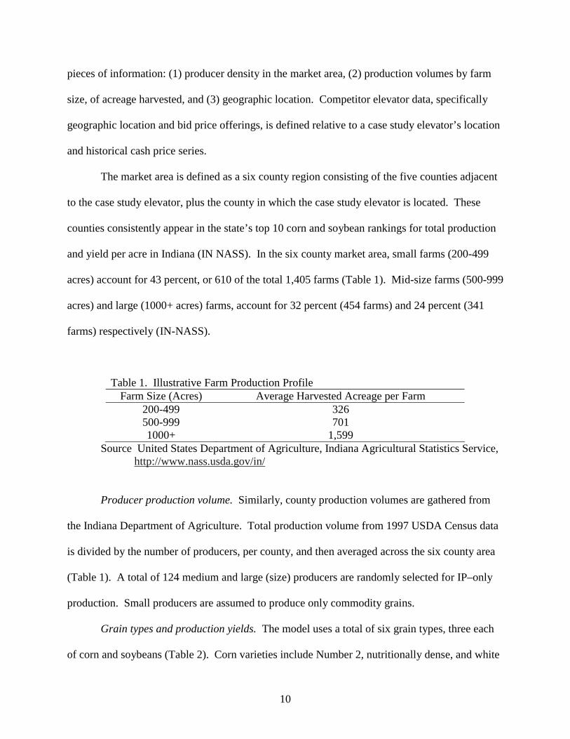
Table 2. Grain Type and Production Yields Grain Type Yield (Bushels per Acre)

Number 2 corn 139 Nutritionally dense 132 White 118 Number 1 soybeans 44 High protein 41 Tofu 38

Source: University of Illinois, Department of Agricultural and Consumer Economics, “The Value Project: Improving Farm Incomes and Rural Communities through Value-Added Agriculture.” http://web.aces.uiuc.edu/value/Default.htm

Producer location. Producers are assumed to be evenly distributed across a circular

market (radius 25 miles) area relative to a case study elevator location. The circular market area

is characterized by 5-mile radial increments along which it is assumed producers are located.

The radial increments are identified a through e, beginning closest to the facility and working

outwards. The circular market area is further divided into quadrants. Thus, producer location is

identified by quadrant and radial increment. The number of small, medium and large producers,

per quadrant per radial increment, is calculated as a percent of harvested acreage each sector

contributes to the quadrant. Each producer has a randomly generated location that is held fixed.

12

A range of possible distances to the grain facility is identified based on intersecting

radials of a particular competitor elevator’s and case study elevator’s locale. A minimum

distance of two miles is established for radial a. Each quadrant contains one competitor grain

elevator in addition to the market area’s centrally located case study elevator.

Transportation. It is assumed that all producers confront the same $ 0.02 per bushel per

mile linear transportation cost as per the 2002 Iowa Farm Custom Rate Survey (Iowa State

University). A transportation cost is calculated for each of the four competing elevators per

producer per week.

Arbitrage Conditions. The distribution of grain flows across facilities is a function of

Equation 1. All grain handling facilities are assumed to confront the same cash price

distribution. However, factors within the firm may afford the firm more, or less, flexibility in the

range of prices they can offer to producers. For example, a facility which can achieve higher

efficiency levels may be able to offer higher bid prices to attract larger volumes to their facility

because they have lowered their cost structure. The elevator’s ability to achieve higher profit

levels is conditioned on maintaining a competitive cost advantage. Should other facilities

achieve similar efficiency levels, the first mover advantage is compromised and possibly even

evaporates. It is also possible that elevator managers are less aggressive with pricing strategies

in high production volume years, where competition has eroded a competitive advantage, or the

grain market returns to a commodity-only scenario.2

Grain facilities are all subject to the same market/cash price and premia per grain type.

The terminal cash price series observed at the case study elevator across fifteen years is the

foundation for competitors’ price series. A weekly, indexed cash price is estimated at the case

2 For example, currently non-GMO grains are classified as IP grains. In the event that demand for non-GMO grains increases so as to rival standard commodity volumes, the previously considered IP grain would become another commodity grain type.

13

study elevator using an empirical distribution. Weekly cash prices are indexed to a 15-year

marketing average to more effectively capture week and year variability. Competitor price

series’ use the case study elevator’s estimated weekly prices as a base; variability is added

through stochastic adjustments to the case study elevator’s price mean and standard deviation.

Price adjustments are based on a probable pricing strategy employed by the competitor given

their type of facility (i.e., small, IP niche market elevator) (Table 3).

Identity preserved premiums are based on 2003 data as provided by the University of

Illinois’s Value Project. The IP corn premiums are $0.22 per bushel (nutritionally dense corn)

and $0.10 (white corn). The IP soybean premiums are $0.90 per bushel (high protein soybeans)

and $1.45 (tofu soybeans).

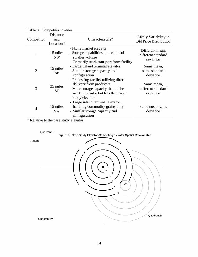
Competitor Location and Distance. Competitor facilities are incorporated into the market

area based on discussions with elevator management. Four types of competitors are identified

(Table 3). Competitor one is assumed to specialize in niche, or IP, market grains, located

approximately 15 miles northwest of the case study elevator (Figure 2, example). Competitor

two is assumed to be a terminal facility of similar storage capacity and bin configuration, relative

to the case study elevator, located 15 miles northeast of the case study elevator. Competitor

three is assumed to be a processor receiving grain deliveries directly from producers and located

approximately 25 miles southeast of the case study elevator. A fourth competitor is a

commodity-only facility situated 15 miles southwest of the case study elevator. Competitor

four’s capacity and configuration closely parallel that of the case study elevator’s.

14

Table 3. Competitor Profiles

Competitor Distance

and Location*

Characteristics* Likely Variability in

Bid Price Distribution

1 15 miles

NW

- Niche market elevator - Storage capabilities: more bins of

smaller volume - Primarily truck transport from facility

Different mean, different standard

deviation

2 15 miles

NE

- Large, inland terminal elevator - Similar storage capacity and

configuration

Same mean, same standard

deviation

3 25 miles

SE

- Processing facility utilizing direct delivery from producers

- More storage capacity than niche market elevator but less than case study elevator

Same mean, different standard

deviation

4 15 miles

SW

- Large inland terminal elevator handling commodity grains only

- Similar storage capacity and configuration

Same mean, same deviation

* Relative to the case study elevator

CE

a

b

c

d

e

Quadrant I Quadrant I

Quadrant IIIQuadrant IV

Figure 2: Case Study Elevator-Competing Elevator Spatial Relationship

Results

15

Results

Results from the grain flow model are presented in Tables 4-8. Results are

interpreted from the case study elevator’s perspective across the premium scenarios.

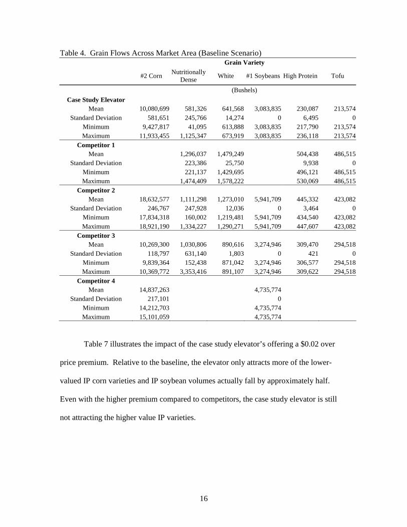
Table 4 presents baseline results which assume no additional premium above the per

bushel market value. Results model suggest absent additional premiums, the case study

elevator would attract all 6 types of grain. Commodity corn and soybean volumes

determined in the model closely resemble actual volumes received. Relative to other

competitors also drawing all 6 grain types, the case study elevator attracts the smallest

absolute volumes. Competitors 1 and 2 are almost equally competitive for IP soybean

grains; competitor 2 is also competes with competitor 4, a commodity-only facility.

Scenario 2 evaluates grain flows when competitor 1 offers an additional $0.02 per

bushel premium (Table 5). The case study elevator draws smaller volumes of both types

of commodity grains and none of the high protein soybeans. Total volume of tofu

soybeans, however, increases almost two fold. Competitor 3’s lack of tofu beans

suggests that producers could have received higher returns at closer distances, thus

distributing tofu volumes among the case study elevator and competitors 1 and 2.

When competitor 2 introduces a $0.02 over-price premium, its volumes of nutritionally

dense and tofu grains increase by over 800,000 and 50,000 bushels respectively, relative

to the baseline scenario (Table 6). Interestingly, this impacts the case study elevator by

increasing all IP volumes except high protein soybeans of which the elevator now

receives none. Presumably, the case study elevator is picking up IP volumes from

quadrant IV of the market area the elevator now receives none.

16

Table 4. Grain Flows Across Market Area (Baseline Scenario) Grain Variety

#2 Corn Nutritionally

Dense White #1 Soybeans High Protein Tofu

(Bushels)

Case Study Elevator

Mean 10,080,699 581,326 641,568 3,083,835 230,087 213,574 Standard Deviation 581,651 245,766 14,274 0 6,495 0

Minimum 9,427,817 41,095 613,888 3,083,835 217,790 213,574 Maximum 11,933,455 1,125,347 673,919 3,083,835 236,118 213,574

Competitor 1 Mean 1,296,037 1,479,249 504,438 486,515

Standard Deviation 223,386 25,750 9,938 0 Minimum 221,137 1,429,695 496,121 486,515 Maximum 1,474,409 1,578,222 530,069 486,515

Competitor 2 Mean 18,632,577 1,111,298 1,273,010 5,941,709 445,332 423,082

Standard Deviation 246,767 247,928 12,036 0 3,464 0 Minimum 17,834,318 160,002 1,219,481 5,941,709 434,540 423,082 Maximum 18,921,190 1,334,227 1,290,271 5,941,709 447,607 423,082

Competitor 3 Mean 10,269,300 1,030,806 890,616 3,274,946 309,470 294,518

Standard Deviation 118,797 631,140 1,803 0 421 0 Minimum 9,839,364 152,438 871,042 3,274,946 306,577 294,518 Maximum 10,369,772 3,353,416 891,107 3,274,946 309,622 294,518

Competitor 4 Mean 14,837,263 4,735,774

Standard Deviation 217,101 0 Minimum 14,212,703 4,735,774 Maximum 15,101,059 4,735,774

Table 7 illustrates the impact of the case study elevator’s offering a $0.02 over

price premium. Relative to the baseline, the elevator only attracts more of the lower-

valued IP corn varieties and IP soybean volumes actually fall by approximately half.

Even with the higher premium compared to competitors, the case study elevator is still

not attracting the higher value IP varieties.

17

Table 5. Grain Flows Across Market Area (Scenario: Competitor 1 pays $0.02 premium/IP bushel)

Grain Variety



(Bushels)

Case Study Elevator

Mean 9,046,997 621,568 749,271 2,744,542 0 421,916 Standard Deviation 578,789 255,090 21,980 2,731 0 12,466

Minimum 8,409,998 60,504 611,042 2,669,853 0 330,224 Maximum 10,915,636 1,086,939 787,615 2,746,210 0 427,148

Competitor 1 Mean 1,339,616 1,489,026 296,267 488,363

Standard Deviation 173,438 41,695 11,233 12,300 Minimum 235,976 1,197,538 221,552 384,400 Maximum 1,505,378 1,630,653 320,913 509,901

Competitor 2 Mean 19,327,574 1,137,663 1,299,802 6,168,383 120,160 462,561

Standard Deviation 249,731 220,064 61,387 5,471 24,818 24,073 Minimum 18,487,976 163,877 1,198,941 6,129,329 88,600 435,791 Maximum 19,628,020 1,738,247 1,849,373 6,170,657 397,242 658,215

Competitor 3 Mean 10,273,568 804,911 615,619 3,277,156 1,026,813 0

Standard Deviation 116,131 568,400 12,833 7,359 17,737 0 Minimum 9,840,215 87,539 495,765 3,273,710 824,447 0 Maximum 10,445,747 3,288,712 622,808 3,462,220 1,053,733 0

Competitor 4 Mean 15,171,700 4,846,183

Standard Deviation 215,717 6,562 Minimum 14,521,210 4,774,863 Maximum 15,455,446 4,882,871

The final scenario evaluates the effect on market grain flows as one competitor

reduces the variability in their $0.01 over premium price (Table 8). Competitor 2’s price

distribution and facility configuration are designed to closely mirror those of the case

study elevator. The impact on the case study elevator is similar to the effects from a

competitor $0.02 premium: commodity volumes fall slightly, the lower-valued IP corn

variety volumes increase and higher-valued IP soybean varieties decrease (in the case of

high protein, they fall to 0). Ultimately, the magnitude of the premium and change in

18

degree of variability will determine the impact on the case study elevator’s grain flows

but it appears that the 2 effects cause the same directional changes for the case study

elevator relative to baseline results.

Table 6. Grain Flows Across Market Area (Scenario: Competitor 2 pays $0.02 premium/IP bushel)

Grain Variety



(Bushels)

Case Study Elevator

Mean 9,046,997 628,250 743,593 2,744,542 0 415,332 Standard Deviation 578,789 253,300 28,356 2,731 0 18,334

Minimum 8,409,998 59,477 609,885 2,669,853 0 291,981 Maximum 10,915,636 1,094,916 791,007 2,746,210 0 427,148

Competitor 1 Mean 1,300,736 1,443,906 285,513 474,024


Competitor 2 Mean 19,327,574 1,196,490 1,355,044 6,168,383 148,805 483,482


Competitor 3 Mean 10,273,568 778,722 611,174 3,277,156 1,008,922 0


Competitor 4 Mean 15,171,700 4,846,183


19

Table 7. Grain Flows Across Market Area (Scenario: Case study elevator pays $0.02 premium/IP bushel)

Grain Variety



(Bushels)

Case Study Elevator

Mean 9,043,687 618,761 551,383 2,743,916 122,352 109,437 Standard Deviation 575,192 435,552 312,596 18,673 107,839 105,290

Minimum 8,409,998 35,384 28,206 2,168,306 8,115 3,238 Maximum 10,915,636 1,805,940 1,308,632 2,744,691 414,611 392,400

Competitor 1 Mean 1,077,450 1,147,846 229,767 224,355

Standard Deviation 446,862 461,070 203,693 186,428 Minimum 79,817 104,740 0 11,027 Maximum 1,720,803 1,763,797 624,630 584,953

Competitor 2 Mean 19,329,419 1,382,085 1,738,636 6,167,384 934,509 890,235

Standard Deviation 247,227 602,596 996,291 29,594 415,835 391,257 Minimum 18,460,108 224,351 210,009 5,276,414 116,125 119,575 Maximum 19,628,020 3,043,517 3,917,884 6,170,657 1,420,636 1,347,242

Competitor 3 Mean 10,274,186 818,644 715,853 3,279,815 156,613 148,812

Standard Deviation 115,214 317,992 238,184 73,174 108,409 102,989 Minimum 9,840,215 139,296 84,898 3,275,229 8,581 8,163 Maximum 10,447,080 1,922,536 957,371 5,513,053 331,680 316,184

Competitor 4 Mean 15,172,548 4,845,150


20

Table 8. Grain Flows Across Market Area (Scenario: Competitor 2 reduces IP premium variability) Grain Variety



(Bushels)

Case Study Elevator

Mean 9,046,997 640,521 757,271 2,744,542 0 427,148 Standard Deviation 578,789 259,420 14,601 2,731 0 0

Minimum 8,409,998 63,475 723,157 2,669,853 0 427,148 Maximum 10,915,636 1,096,385 791,007 2,746,210 0 427,148

Competitor 1 Mean 1,313,676 1,458,515 288,879 478,691


Competitor 2 Mean 19,327,574 1,162,818 1,318,373 6,168,383 137,394 467,000


Competitor 3 Mean 10,273,568 787,491 619,559 3,277,156 1,016,968 0


Competitor 4 Mean 15,171,700 4,846,183


Conclusions

This paper has examined grain flow distributions across an illustrative market in

north central Indiana from a case study elevator’s perspective. Arbitrage conditions are

employed by producers to determine their best delivery option, represented by the highest

return net of assembly costs.

In general, near-by competitors offering a $0.02 over price premium result in

decreased volumes of higher-valued high protein soybeans but increased volumes of the

21

highest-valued tofu variety by almost twice as much. Smaller premiums associated with

IP corn varieties are equally as distance-sensitive; the case study elevator’s location

makes them an attractive delivery site for producers who receive smaller premiums to

offset transport costs. This paper highlights the relationship between linear transportation

costs and IP premium structures confronting the producer. Results suggest that the

distance threshold for IP grains with smaller premiums is closer than it is for higher

premium types. This paper began on the assumption that IP premiums would influence

producer delivery decisions. Findings indicate that the elevator manager’s need to be

aware of the magnitude of variety premiums in assessing changes to their grain flows.

Across premium scenarios, commodity volumes changed only nominally. This is

expected in that they are only indirectly affected by IP market premiums. The underlying

issue however is the cost in operational efficiency as the IP grains are added to an

individual elevator’s facility. Examination of the costs of incorporating IP grains into a

facility’s product mix will involve evaluation of the economics costs of adding additional

grain types, with attribute preservation requirements to a commodity-system.

22

Bibliography

Araji, Ahmed A. and Richard G. Walsh. “Effect of Assembly Costs on Optimum Grain

Elevator Size and Location.” Canadian Journal of Agricultural Economics. 3(17): 36-45, 1969.

Baker, S. T. Herrman, and F. Fairchild. “Capability of Kansas Grain Elevators to

Segregate Wheat During Harvest.” Progress Report n. 781, Kansas Agricultural Experimental Station, KS. 1997.

Berruto, Remigio and D.E. Maier. “Analyzing the Receiving Operation of Different

Grain Types in a Single Pit Country Elevator.” Transaction of ASAE, 44(3): 631-638. 2001.

Berruto, Remigio and D.E. Maier. “Using Object Oriented Modeling Techniques to Test

the Feasibility of GMO Grain Segregation and Traceability at Commercial elevators.” IFAC Conference, Modeling and Control in Agriculture, Horticulture and Post-harvest Processing, 12-14 July 2000, Wageningen, The Netherlands.

Davis, L., and L.D. Hill. “Spatial Price Differentials for Corn and Among Illinois

Country Elevators.” American Journal of Agricultural Economics. 56:135-144, 1974.

Dooley, Frank J. and Wesley W. Wilson. The Effect of Elevator Competition Upon

Market Areas. Journal of the Transportation Research Forum. 28(1): 120-125, 1987.

Herrman, T. and Mike Boland. “Segregation Strategies.” Feed & Grain, 20-24:

February/March 1999. Hurburgh, Charles R., Jr. “Identification and Segregation of High-Value Soybeans at a

Country Elevator.” Journal of American Oil Chemists Society. 71(10):1073-1078. October 1994.

Hurburgh, Charles R., Jr., Jeri L. Neal, Marty L. McVea, and Phillip Baumel. “The

Capability of Elevators to Segregate Grain by Intrinsic Quality.” Presentation at 1994 American Society of Agricultural Engineers Summer Meeting. 1994.

Jones, D. “An Economic Analysis of the Relationship Between Market Structure

Variables and Price Differentials Among Illinois Country Elevators.” Masters Thesis. University of Illinois at Urbana-Champaign. 1971.

Krueger, Angela, Frank Dooley, Remigio Berruto, and Dirk Maier. “Risk Management

Strategies for Grain Elevators Handling Identity-Preserved Grains.” Selected Paper. International Agribusiness and Management Association World Conference. Chicago, Illinois. June 2000.

23

Maltsbarger, Richard. “The Ability of Elevators to Intermediate Identity-Preserved Supply Chains.” Thesis, Department of Agricultural Economics. University of Missouri-Columbia. December 1999.

McCully, M. “An Econometric Analysis of the Market Structure Variables and Their

Impact on Market Performance of Illinois Grain Elevators.” Masters Thesis. University of Illinois at Urbana-Champaign.

McVey, Marty, Baumel, C. Phillip, and Hurburgh, C.R. Jr. “Efficient Distribution Of

Grain To Meet The Quality Needs Of End-Users.” Midwest Transportation Center, Iowa State University, Ames, 1996.

Sonka, Steven, R. Christopher Schroeder, and Carrie Cunningham. “Trasportation,

Handling and Logistical Implications of Bioengineered Grains and Oilseeds: A Prospective Analysis.” Agricultural Marketing Service, United States Department of Agriculture. November 2002.

United States Department of Agriculture, Indiana Agricultural Statistics Service,

http://www.nass.usda.gov/in/ University of Illinois, Department of Agricultural and Consumer Economics, “The Value

Project: Improving Farm Incomes and Rural Communities through Value-Added Agriculture.” http://web.aces.uiuc.edu/value/Default.htm

Wenzel, Benjamin P., Lowell Hill, and Philip Garcia. “The Effects of Micro-Market

Structure on Illinois Elevator Spatial Corn Price Differentials.” NCR-134 Conference on Applied Commodity Price Analysis, Forecasting, and Market Risk Management. Chicago, IL. April 17-18, 2000.

Documents

The Effect of Identity Preserved Premiums on Elevator ...ageconsearch.umn.edu/bitstream/21955/1/sp03gl01.pdf · The effect of identity preserved premiums on a grain ... of Identity