1

THE EFFECT OF HALF-SHAFT TORSION DYNAMICS ON THE

PERFORMANCE OF A TRACTION CONTROL SYSTEM FOR ELECTRIC

VEHICLES

F. Bottiglione

Politecnico di Bari, DIASS (Visiting Researcher at the University of Surrey for the

project described in this article)

Via A. De Gasperi s/n Viale Japigia 182

74100 Taranto

Italy

A. Sorniotti, L. Shead

University of Surrey

Guildford, Surrey GU2 7XH

United Kingdom

Abstract

This article deals with the dynamic properties of individual wheel electric powertrains

for fully electric vehicles, characterised by an in-board location of the motor and

transmission, connected to the wheel through half-shafts. Such a layout is applicable to

2

vehicles characterised by larger power and torque requirements where the adoption of

in-wheel electric powertrains is not feasible due to packaging constraints. However, the

dynamic performance of in-board electric powertrains, especially if adopted for anti-

lock braking or traction control, can be affected by the torsional dynamics of the half-

shafts. This article presents the dynamic analysis of in-board electric powertrains in

both the time and frequency domains. A feedback control system, incorporating state

estimation through an extended Kalman filter, is implemented in order to compensate

the effect of half-shaft dynamics. The effectiveness of the new controller is

demonstrated through the analysis of the performance improvement of a traction control

system.

Keywords

In-board electric powertrain; half-shaft torsional compliance; traction control.

1. Introduction

The traditional layout of electric vehicle powertrains consists of a central motor, a

single-speed or multiple-speed transmission, a differential and half-shafts [1-4].

However, the future of electro-mobility is likely to be based on the adoption of

individually controlled powertrains for each wheel [5]. From the viewpoint of vehicle

dynamics, this solution provides significant advantages, due to the possibility of

3

implementing direct yaw moment control for the enhancement of vehicle response in

steady-state and transient conditions [6-8], and for the actuation of anti-lock brake

system (ABS) and traction control (TC) functions. This is achievable through the

precise control of the electric powertrain torque at the wheel. However, current

regenerative braking systems for electric powertrains usually leave the modulation of

the braking torques to the friction brakes, and reduce the regenerative action during

ABS cycling [9-11], whilst traction control systems based on the actuation of internal

combustion engines are characterised by a relatively low bandwidth. The low reaction

time and high bandwidth of electric motor drives potentially allow the development of

ABS controllers based on direct slip control [12-17] instead of the conventional hybrid

controllers based on the combination of wheel acceleration control and wheel slip

control [18].

Individual in-wheel electric powertrains provide an additional benefit from the

viewpoint of the design of the overall vehicle chassis, by permitting an increase of the

available volume in the area between the wheels. However, current motor technology is

limited in terms of power and torque density, which makes in-wheel powertrains, with

their motor drive unit incorporated into the vehicle unsprung mass, a viable solution

only for small and medium size cars, with relatively low performance. Despite recent

studies [19-20] which suggest a past overestimation of the importance of this factor, in-

wheel electric powertrains are associated with an undesired increase of vehicle

4

unsprung mass, with the subsequent ride comfort and vehicle dynamics implications

(for rough road conditions). Moreover, the adoption of an in-wheel powertrain on the

wheels of a steering axle increases the turning radius of the vehicle, due to the related

packaging issues.

As a consequence, a possible solution for the implementation of individual electric

powertrains, without being subject to the limitations of the in-wheel layout, is the

implementation of in-board electric powertrains. These are characterised by a motor

drive and a transmission connected to the vehicle chassis through a powertrain

mounting system (possibly including bushings with non-linear elastic and damping

properties), and by a half-shaft with constant velocity joints for driving the wheel.

However, the main disadvantage of the in-board electric powertrain arises from the

torsional dynamics of the half-shaft and the subsequent first torsional mode of the

powertrain. The torsional dynamics of the electric drivetrain is due to the fact that the

half-shaft can be considered as the combination of a torsion spring and damper (with

very low damping ratio) in parallel, connecting the equivalent mass moment of inertia

of the drivetrain to the inertia of the wheel. Moreover, the torsional dynamics of the

system are significantly affected by the slip ratio dynamics of the tyres, due to the

combination of tyre steady-state non-linear characteristics and relaxation length. In a

first approximation, tyres can be represented as non-linear dampers within the system.

Also the dynamics of the electric powertrain mounting system, especially if the

5

drivetrain includes bushings, is relevant to vehicle drivability, because of the forces

transmitted to the vehicle chassis by the powertrain mounting system. All these

phenomena could interfere with vehicle drivability, by affecting jerk dynamics, as is

well known for internal combustion engine driven vehicles [21], usually characterised

by a first natural frequency of the powertrain between 4 and 7 Hz. The torsional mode

of the powertrain could also reduce the effectiveness of ABS and TC actuation.

However, the literature about electric vehicle control has not investigated this aspect

yet.

This article provides a comprehensive analysis of the dynamics of in-board electric

powertrains, in both the frequency and time domains. A potential limitation in the

actuation of effective ABS and TC systems is demonstrated. A feedback controller,

based on an extended Kalman filter [22] for the estimation of the half-shaft torque, is

implemented for the compensation of half-shaft torsional dynamics during ABS and TC

intervention, which is a novel control approach for this important application. A similar

algorithm has been implemented in [23] for the compensation of the effect of the

transmission plays on electric vehicle drivability.

2. The Simulation Model

This section describes the basic principles of the implemented non-linear model of the

longitudinal dynamics of a case study front-wheel-drive vehicle with individually

6

controlled powertrains. A non-linear powertrain model is developed (and subsequently

used as a simulator), from which a linearised vehicle model is derived for controller

design purposes. The model presented in this section includes a significant number of

simplifications, and has been selected as the simplest non-linear model capable of

reproducing the dynamics of interest for the specific application [21].

Figure 1 is the schematic of an individual wheel powertrain, characterised by a three-

stage single-speed transmission with a layshaft layout. The equivalent mechanical

model implemented in this article consists of three degrees of freedom: the vehicle, the

wheel and the powertrain. The half-shaft is modelled as a torsion spring and damper

with two mass moments of inertia at its ends. The damping coefficient of the half-shaft

is low due to the very small internal damping of the material (steel). The connection

between the wheel and the equivalent inertia of the vehicle is represented by the tyre.

The angular speeds of the wheel and the equivalent inertia of the vehicle differ because

of the slip ratio.

7

Figure 1 – Schematic of the individual in-board electric powertrain with a zoomed view

of the three-stage single-speed transmission

The electric motor reaction time and slew rate are included in the simulation model. The

specific motor drive unit of this vehicle application is of a switched reluctance topology,

characterised by a particularly low value of mass moment of inertia. A small time

constant τM takes into account the effect of the electric dynamics of the motor (due to its

equivalent circuit parameters):

,M M M M refτ T T T (2.1)

Equation (2.2) models the overall powertrain dynamics from the motor shaft to the

transmission output shaft. A look-up-table based model is adopted for the estimation of

the windage losses Twindage, which are functions of the rotor angular velocity:

8

22

1 21 2 3 1

1 2 3

1 2 3 1 1 1 2

g gg g g g

M windage HS M

j

i ii i i iT T T J J J J

η η η η η η η

2

1 2 3

4

1 2 3 1

1

2

g g g HSM

j

i i i JJ θ

η η η η

(2.2)

where half-shaft torque THS is given by:

1 2 3 1 2 3 FWHS HS g g g M FW HS g g g MT β i i i θ θ k i i i θ θ

(2.3)

Transmission efficiency is modelled through a look-up-table-based model, as a function

of the input torque, speed and operating temperature. Starting from THS, equation (2.4)

calculates the net torque TFW transmitted by the half-shaft to the wheel:

2 2

FW HSHS FW

j

T JT θ

η (2.4)

Equation (2.5) is the rotational equilibrium of the driven wheel:

, , ,FW d FW r F z FW W FW FWT T f F R J θ (2.5)

Tyre rolling resistance coefficient fr is modelled as a parabolic function of the tangential

speed of the wheel. Tyre longitudinal force Td,FW/RW is modelled using the Pacejka

magic formula [24], including a relaxation length model for the evaluation of the

transient effects, according to equation (2.6):

, , ,

tyre

d FW d FW FW Pacejka

FW W

LT T T

θ R (2.6)

Ltyre is a function of wheel speed, tyre vertical load and slip ratio.

9

Vehicle longitudinal dynamics are modelled through an equivalent moment of inertia,

which is subject to equivalent torques due to the aerodynamic drag and the driven and

undriven (the rear ones for the specific case study vehicle of this article) wheels.

Equation (2.7) describes the dynamics of the equivalent inertia of the vehicle:

3 2 2

, , ,

12 2 2

2d FW r R z RW W d W V RW W VT f F R ρC SR θ J mR θ (2.7)

Given the focus of the activity, the wheel vertical load transfers due to the longitudinal

acceleration and deceleration levels have been computed considering neither the effect

of suspension stiffness and damping, nor tyre vertical dynamics. For example, the

vertical load on each front wheel is equal to:

2

,

2

1

2 4

2

RWz FW W d CG m

FW RW FW RW

CGl RW V W V

FW RW

b uF mg ρSR C h C L

L u u L u u

hC b u θ m R θ

L u u

(2.8)

A similar equation is adopted for the computation of the vertical load on the rear axle.

The most relevant vehicle data are included in Table B.1 of Appendix B.

Linearization permits the analysis of the frequency response of the system and control

system design. The model described by equations (2.1)-(2.8) has been subject to

linearization around an operating condition, defined by a value of vehicle velocity and

slip ratio. In the linear model, the tyre is considered as an equivalent torsion damper

between the wheel and vehicle inertia, where the equivalent damping coefficient is

10

obtained through the linearization of the Pacejka magic formula around the selected

operating point. The main non-linearities of the system are due to the tyre force

characteristics. In particular, the absolute value of tyre longitudinal slip stiffness is

positive and progressively decreasing from the condition of zero slip until the peak

value of longitudinal force, at which it assumes a null value. When the longitudinal slip

stiffness of the tyre is null, the individual powertrain dynamics are completely

decoupled from the dynamics of the equivalent inertia of the vehicle. This offers the

theoretical justification of the simplification carried out by most authors (for example,

[12]) in the derivation of the dynamic equation of the slip ratio within the

implementation of model-based ABS. Wheel dynamics are much more pronounced and

at higher frequency values than vehicle longitudinal dynamics for conditions of slip

ratios around the value generating the peak longitudinal tyre force. Beyond the peak

longitudinal force, tyre longitudinal slip stiffness is negative. The linearised model has

been implemented in a state-space formulation:

X AX BU

Y CX DU

(2.9)

The detailed mathematical formulation of the elements of the X and U vectors and the A

and B matrices defined in equation (2.9) is included in Appendix A, with some marginal

additional simplifications (e.g. the windage losses are neglected). Additionally, it is

possible to predict that most in-board implementations of electric powertrains will be

11

usually characterised by a lower length of the half-shafts (in comparison with internal

combustion engine driven powertrains), due to the width of the system formed by the

two electric motor units per each axle.

Assuming some particular vehicle parameters (Appendix B), the frequency response of

the model has been analysed for a number of different linearization points, given the

absence of any literature about the frequency response of such a powertrain layout.

Figure 2 contains the Bode plots of the adimensionalized half-shaft torque response to

an input motor torque, for different values of slip ratio (linearization point), and two

values of half-shaft length (i.e. half-shaft torsion stiffness), at a vehicle velocity of 50

kph, in conditions of high friction coefficient (μ = 1) between the tyre and the road

surface. ig* is the overall single-speed transmission ratio (ig

* = ig1ig2ig3). At low values of

slip ratio (graphs at null slip ratio in the figure), the frequency response is characterised

by two peaks, at the natural frequencies of the system. The first one is visible in the

diagrams, and is located between 80 and 90 rad/s (about 13 and 14 Hz), whilst the

second peak is not visible, as it is located beyond the frequency limits of the plot. When

the value of slip ratio at the linearization point is increased to 0.05, the low frequency

peak in the half-shaft torque response is subject to an amplitude reduction. Moreover,

the frequency of the second resonance peak gets lower, and the two peaks become

closer. This is the range of slip ratios usually relevant for vehicle drivability. Finally, for

values of slip ratio close to the one corresponding to the peak longitudinal tyre force,

12

the system experiences a significant resonance peak between 100 and 200 rad/s (about

16 and 32 Hz). The frequency range of ABS modulation in common systems based on

the hydraulic actuation of the friction brakes is between 4 and 7 Hz. According to [25],

the adoption of in-wheel motors can increase the ABS modulation frequency up to 9-10

Hz. This is the range of interest of this simulation model. Beyond these limits, there

could be modal interactions with the longitudinal motion of the wheel relative to the

chassis, due to suspension compliance, usually in the region of 40-100 Hz [26].

(a) (b)

Figure 2 – Bode plot (magnitude and phase) of the adimensionalized half-shaft torque

for an input torque request, at different values of tyre longitudinal slip ratio (continuous

line) 0.0, (dashed line) 0.05, (o) 0.1, (□) 0.138 (peak), (∆) 0.15. Vehicle speed is 50 kph.

13

Two half-shaft lengths are shown: (a) lHS = 506 mm, (b) lHS = 360 mm

Figure 3 plots the sensitivity of the frequency response of the same electric powertrain

to different values of the tyre-road friction coefficient, for a relatively low slip ratio (σ =

0.05, Figure 3(a)), relevant to vehicle drivability, and a slip ratio close to the one

corresponding to the peak value of tyre longitudinal force (σ = σPEAK - 0.01, Figure

3(b)). The frequency response of the system is strongly dependent on μ, with the only

exception being represented by the case of system linearization at exactly σPEAK, where

all the Bode plots (for whatever μ) are coincident. In fact, in that condition wheel

dynamics are decoupled from vehicle dynamics, and so the tyre longitudinal slip

stiffness is equal to zero. In the analysis of this preliminary research activity, the

variation of the shape of the tyre force characteristic as a function of μ has been

neglected (all the characteristics have been scaled down according to the assigned

friction coefficient) and the existence of the peak of tyre longitudinal force has been

considered also in conditions of very low friction. Future analysis will have to

investigate the frequency response of the system in case of low friction surface with

snow, which gives rise to a monotonically increasing tyre force characteristic as a

function of the slip ratio.

In conclusion, the case study individual wheel powertrain is characterised by a higher

value of the first natural frequency than the powertrain of an internal combustion engine

14

driven vehicle, which results in an improvement of vehicle drivability. However, the

open-loop dynamic response of the powertrain, due to the torsional dynamics of the

half-shafts, is not satisfactory for ABS and TC based on direct slip control. For

example, [12] mentions a bandwidth of 72 rad/s (about 11.5 Hz) for the electro-

mechanical friction brake callipers adopted in that specific vehicle application.

(a) (b)

Figure 3 – Bode plot (magnitude and phase) of the adimensionalized half-shaft torque

for an input torque request, at different values of tyre-road friction coefficient μ and

with a longitudinal slip ratio σ given by: (a) σ = 0.05, (b) σ = σPEAK - 0.01. Vehicle speed

is 50 kph. lHS = 506 mm

3. Control System Design in the Frequency Domain

15

Figure 4 is the linearized block diagram of a TC based on slip ratio feedback control

without any compensation of half-shaft torque dynamics, similar to the system

presented in [27]. The estimation of the slip ratio implies the availability of precise

information of vehicle longitudinal velocity, which can be easily derived, for the case of

a two-wheel-drive vehicle, from the wheel speed sensors of the undriven wheels, which

would be adopted in any case for the purpose of anti-lock braking control. This method

for the estimation of vehicle speed is reasonably reliable also in case of cornering

conditions. The main non-linearities of the control system are represented by the switch

for the activation and deactivation conditions based on two different slip ratio

thresholds, and by the fact that during TC activation the algorithm selects the lower

between the driver torque demand and the output torque from the traction control

system.

In the frequency domain, for a vehicle with a traction control system based on direct slip

control implemented through a Proportional Integral Derivative (PID) controller, tyre

slip ratio σ s is given by:

, ,

,1

ref PID TC M ref PLANT

PID TC PLANT

σ s K s T s G sσ s

K s G s

(3.1)

The slip ratio is due to the combination of the reference torque contribution ,M refT s

imposed by the driver and the torque correction calculated by the traction controller. For

a first approximation design of the tracking performance of the traction controller, it is

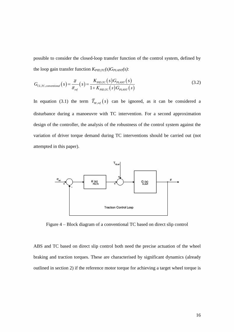
16

possible to consider the closed-loop transfer function of the control system, defined by

the loop gain transfer function KPID,TC(s)GPLANT(s):

,

, ,

,1

PID TC PLANT

CL TC conventional

ref PID TC PLANT

K s G sσG s s

σ K s G s

(3.2)

In equation (3.1) the term ,M refT s can be ignored, as it can be considered a

disturbance during a manoeuvre with TC intervention. For a second approximation

design of the controller, the analysis of the robustness of the control system against the

variation of driver torque demand during TC interventions should be carried out (not

attempted in this paper).

Figure 4 – Block diagram of a conventional TC based on direct slip control

ABS and TC based on direct slip control both need the precise actuation of the wheel

braking and traction torques. These are characterised by significant dynamics (already

outlined in section 2) if the reference motor torque for achieving a target wheel torque is

17

purely calculated by the ABS or TC as the desired wheel torque multiplied by the

transmission gear ratio (<1 according to the conventions adopted in the article).

The idea of this research is the implementation of an inner control loop for the feedback

compensation of the torque oscillations at the wheels (Figure 5). The feedforward

component of the reference torque at the half-shaft is computed as the reference electric

motor torque *

,M refT , depending on driver input and the traction control, divided by ig*.

Figure 5 – Block diagram of the TC based on direct slip control as the outer control loop

and the feedback controller for the compensation of half-shaft torque dynamics as the

inner control loop, including the schematic detailing the input and output signals of the

extended Kalman filter for half-shaft torque estimation

18

A PID controller has been implemented for the feedback control of half-shaft torque as

the inner control loop, according to the linearized block diagram of the system of Figure

6. The gains have been designed for the achievement of about 7 dB of gain margin and

60° of phase margin, at a vehicle velocity of 50 kph.

As half-shaft torque cannot be directly measured on the plant, the system requires the

implementation of an extended Kalman filter (Figure 5), for the estimation of the half-

shaft torque level. The extended Kalman filter is based on the non-linear electric

powertrain model presented in section 2, with the exclusion of tyre relaxation length

and the equations of the longitudinal vehicle dynamics. Appendix C presents the

structure and the details of the formulation of the extended Kalman filter adopted in this

contribution. The measured values of the angular velocities of the motor and the wheel

and the measurement of the motor torque have been provided through sensor simulation

and were pre-conditioned with properly tuned low-pass filters. The selection of the

noise level for the measurements has been carried out consistently with the experimental

values reported in [12]. This Kalman filter can also provide a reliable estimation of tyre

longitudinal force, being characterised by a non-linear tyre model. An alternative

implementation of a similar Kalman filter is presented in [23], where the filter is

simplified from the viewpoint of the estimation of tyre force, but includes, within its

non-linear model, the simulation of transmission plays, which can provoke significant

19

driveline oscillations. The best option for the detailed implementation of the Kalman

filter will be experimentally verified by the authors during the vehicle testing activity

which is going to be implemented in future.

A comprehensive set of simulations has been carried out in order to check the

robustness of the extended Kalman filter estimation against the variation of tyre-road

friction coefficient, and against the variation of tyre parameters. In particular, for the

specific case study, the filter estimation is not significantly affected even by an incorrect

estimation of tyre friction coefficient, when the slip ratio is not close to the value

corresponding to the peak longitudinal force. Therefore, within the implementation, the

extended Kalman filter is fed with a fairly crudely estimated value of the actual tyre

friction utilisation, based on the methodology presented in [27].

The new feedback controller is useful during normal driving conditions for improving

vehicle drivability, and during TC or ABS actuation for improving wheel dynamics. If

we ignore the dynamics induced by the presence of the Kalman filter on the feedback

loop, the loop gain transfer function for the system including the new control loop is:

)()()(1

)(1

)()()(

,

,,

*

,

,

,,,

sKsGsKi

sKG

sKsKGsG

TCPID

HSPLANTHSPIDg

HSPID

PLANT

TCPIDCLHSPLANTLG

(3.3)

At the moment, within this research focused on the analysis of the in-board powertrain

dynamics, the traction control system does not include a robust adjustment of σref as a

function of the estimated tyre characteristics. As the focus of this article is on the effect

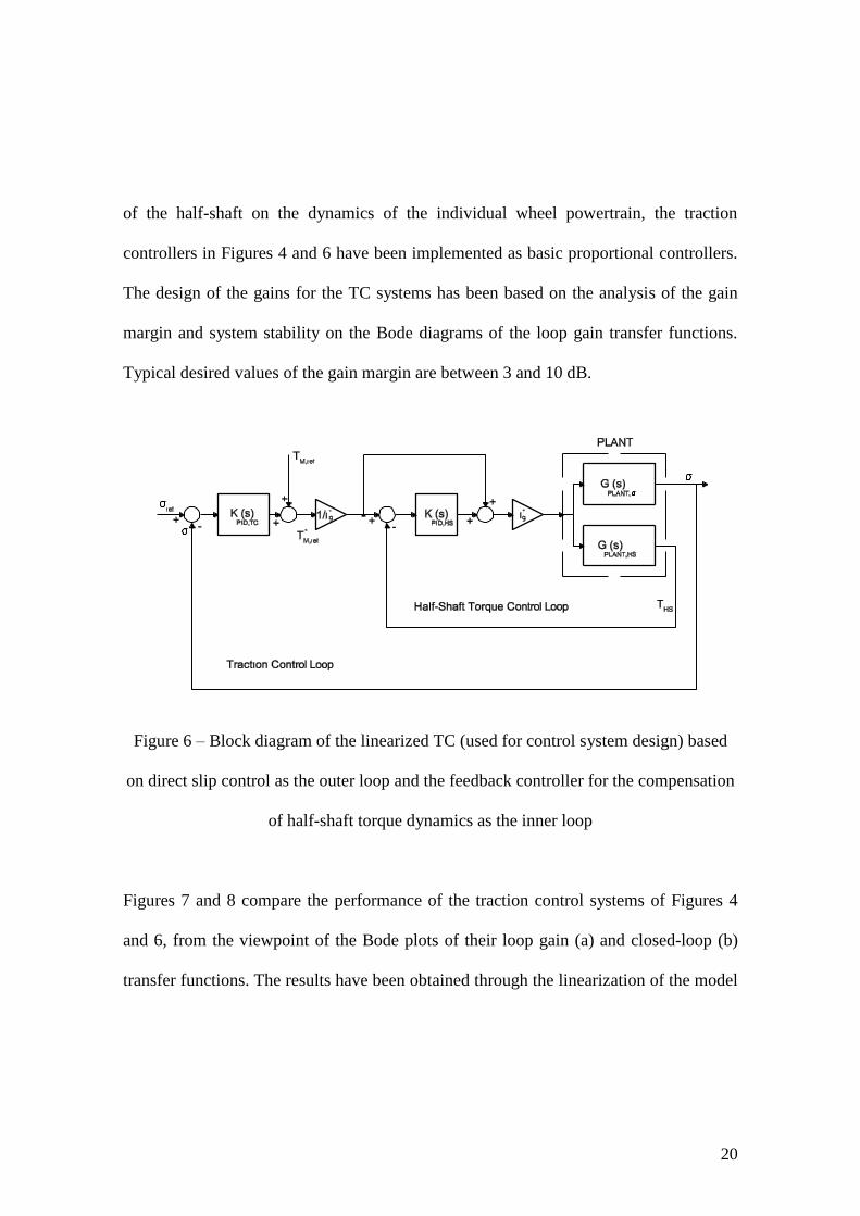
20

of the half-shaft on the dynamics of the individual wheel powertrain, the traction

controllers in Figures 4 and 6 have been implemented as basic proportional controllers.

The design of the gains for the TC systems has been based on the analysis of the gain

margin and system stability on the Bode diagrams of the loop gain transfer functions.

Typical desired values of the gain margin are between 3 and 10 dB.

Figure 6 – Block diagram of the linearized TC (used for control system design) based

on direct slip control as the outer loop and the feedback controller for the compensation

of half-shaft torque dynamics as the inner loop

Figures 7 and 8 compare the performance of the traction control systems of Figures 4

and 6, from the viewpoint of the Bode plots of their loop gain (a) and closed-loop (b)

transfer functions. The results have been obtained through the linearization of the model

21

in an operating condition close to the peak point of the longitudinal force characteristic

of the tyre (precisely at a slip ratio with an offset of 0.01 to the left of the peak slip

ratio), at a vehicle velocity of 50 kph. The adoption of the half-shaft torque control inner

loop provides a significant enhancement of system stability. This allows the selection of

higher values of the proportional gain of the TC, resulting in a quicker dynamic

response of the controller, for the same values of gain margin, which are compared in

Table 1 for different tunings of the proportional gain of the TC. Table 1 also shows a

significant increase of the gain margin as a function of vehicle velocity, which implies

the requirement for a gain scheduling of the controller. Due to the high non-linearity of

the system, the fine tuning of the controller requires simulations in the time domain,

which are presented in section 4. Figures 7(b), 8(b) and 9 compare the closed-loop

performance of the control systems of Figures 4 and 6 in the frequency domain. In

particular, with the system including the feedback controller on half-shaft torque, it is

possible to achieve an acceptable tracking capability (-3.5 dB of closed-loop response)

up to a frequency of about 47 Hz, well beyond the expected frequency range for TC and

ABS. Additional benefits should be achievable by adopting more advanced controllers

for the TC function, such as compensators and linear quadratic regulators, which will be

the object of future research.

22

(a) (b)

Figure 7 – Bode plots of the (a) loop gain transfer function and the (b) closed-loop

transfer function of the vehicle including traction control and excluding the half-shaft

torque control. The frequency response plots are shown for different values of the

proportional gain of the traction control: (continuous) 10 Nm, (dashed) 50 Nm, (o) 100

Nm, () 300 Nm, (▲) 700 Nm

23

(a) (b)

Figure 8 – Bode plots of the (a) loop gain transfer function and the (b) closed-loop

transfer function of the vehicle including traction control and the half-shaft torque

control. The frequency response plots are shown for different values of the proportional

gain of the traction controller: : (continuous) 10 Nm, (dashed) 50 Nm, (o) 100 Nm, ()

300 Nm, (▲) 700 Nm

P Gain [Nm]

10 50 100 300 700

Without half-shaft torque control

20 kph - 6.34 -20.3 -26.3 -35.9 -43.2 50 kph 7.82 -2.16 -12.2 -21.7 -29.1 90 kph 15.2 1.26 -4.76 -13.3 -21.6

With half-shaft torque control

20 kph 36.6 22.7 16.6 7.1 -0.27 50 kph 44.6 30.6 24.6 15.1 7.7 90 kph 49.8 35.8 29.8 2.2 12.9

Table 1 – Gain margin values (in dB) for different tunings of the

24

proportional gain (P Gain) of the traction control system

Figure 9 – Bode magnitude plot of the closed-loop transfer function of the system with

traction control, excluding inner loop (marked with □) and including inner loop (marked

with o), at two different values of vehicle speed: 40 kph (dashed line), 80 kph

(continuous line). The proportional gain of the traction control is equal to 17 Nm in the

system without the half-shaft torque control loop and it is 700 Nm in the system with

inner loop

Figure 10 is the root locus plot for the overall closed-loop system, excluding (Figure

10(a)) and including (Figure 10(b)) the half-shaft torque control system. The adoption

of the novel half-shaft torque control system cancels the poles near the imaginary axis

and moves the part of the root locus which progresses towards the right-hand plane

25

(RHP) zeros (not pictured) further to the left. This significantly contributes to system

stability, allowing the adoption of higher values of the proportional gain of the traction

control system.

(a) (b)

Figure 10 – Root locus analysis excluding and including half-shaft torque control at 50

kph

4. Results in the Time Domain

The half-shaft torque inner control loop presented in section 3 is a useful method for

modifying the loop gain frequency response such that TC/ABS slip (or anti-jerk) control

design is much simpler and provides higher performance.

26

Figure 11 demonstrates the functionality of the novel controller through simulation in

the time domain. The electric motor torque (and hence the reference wheel torque) is

ramped up to a desired steady-state level, and then a sinusoidal oscillation at a

frequency of 9 Hz is superimposed. In Figure 11(a), the vehicle equipped with the

control system can follow the reference, whilst the vehicle without the feedback control

system on half-shaft torque suffers from a mean level offset, a phase lag, and a

significant amplitude error in the oscillations.

(a) (b)

Figure 11 – Half-shaft reference torque (thin continuous line), actual half-shaft torque

(thick continuous line) and Kalman filter estimation of half-shaft torque (dashed line)

with half-shaft torque control (a) and with no control (b). The electric motor drive

reference torque (whilst in the figure half-shaft torques are plotted) is a step of 70 Nm

plus a sinusoidal oscillation with an amplitude of 10 Nm and a frequency of 9 Hz.

Vehicle initial velocity is 50 kph

27

Simulations of tip-in tests (Figure 12) with the non-linear model show the typical

oscillations of the vehicle acceleration profile induced by the torsional dynamics of the

electric powertrains. The vehicle equipped with the feedback half-shaft torque controller

is characterised by an appreciably smoother acceleration profile, with attenuated

oscillations in comparison with the vehicle without the novel control system, and so the

controller can be considered as an indirect anti-jerk controller.

Figure 12 – Vehicle longitudinal acceleration profile during a tip-in manoeuvre with

half-shaft torque control (continuous line) and without half-shaft torque control (dashed

line). Final torque demand of 75 Nm per electric motor starting from zero. Initial

vehicle speed of 20 kph

28

Finally, Figure 13 is the comparison of the performance of the passive vehicle, the

vehicle equipped with the TC of Figure 4 (according to two different tunings) and the

vehicle equipped with the TC and the half-shaft torque control system of Figure 6,

during a tip-in test from an initial speed of 50 kph. The wheel torque level during the

first part of the tip-in manoeuvre is beyond the friction limit of the tyres, which implies

significant wheel spinning for both the passive vehicle and the vehicle with TC only

(proportional control). The TC without half-shaft torque control requires a significantly

low value of the proportional gain of the controller for keeping system stability, as

discussed in section 3. The stand-alone TC based tuned according to the system

frequency response characteristics was unable to achieve the desired performance level

with a proportional gain only. Therefore, a PID control system has also been

implemented replacing the TC gain controller (still without the inner half-shaft torque

control loop) in order to reduce the slip ratio especially during the first part of the wheel

spinning phase.

In frequency domain terms, the PID controller can be utilised as a band-stop

compensator to reduce the loop gain around the first resonant peak in order to improve

the gain margin. In any case, even this TC configuration achieves a more irregular slip

control dynamics in comparison with the system including the half-shaft torque inner

control loop. The vehicle equipped with the novel controller and a basic proportional

29

TC is characterised by the absence of any significant wheel spinning (maximum slip

ratio of about 0.16) and a higher velocity profile than the other three vehicles.

Figure 13 – Wheel (continuous line) and vehicle velocities (dashed line) during a tip-in

manoeuvre. Vehicle without control system (▲); vehicle with traction control based on

a proportional gain (*); vehicle with traction control based on a PID controller ();

vehicle with traction control based on a proportional gain and the novel half-shaft

torque control (o)

The main performance metrics relating to the manoeuvre of Figure 13 are reported in

Table 2. In particular, the novel controller proposed in this contribution allows the

achievement of an average value of slip ratio very close to the reference, with a

30

reduction of the peak values of the longitudinal slip ratio by a percentage between 85%

and 116% in comparison with the vehicles equipped with traction control systems

without the half-shaft torque feedback loop.

No control

Proportional

gain traction

control

PID traction

control

Proportional

gain traction

control with

half-Shaft

torque

control

Average

acceleration 1.36 m/s

2 1.39 m/s

2 1.51 m/s

2 1.58 m/s

2

Average slip

ratio 0.262 (+113%) 0.239 (+94%) 0.152 (+24%) 0.123

Peak slip ratio 0.403 (+129%) 0.38 (+116%) 0.325 (+85%) 0.176

Table 2 – Performance metrics of the different traction control solutions presented in the

paper, during the same manoeuvre as in Figure 13. The percentage variations are

referred to the proportional traction control system including half-shaft torque control

(configuration in the last column on the left in the table)

5. Conclusion

The article has demonstrated the potential effects induced by the torsional dynamics of

the half-shafts on the response of individual wheel in-board powertrains. In particular,

the first natural frequency of the system, due to the torsional stiffness of the half-shaft,

the mass moments of inertia of the powertrain components and the tyre characteristics at

31

the operating point, is responsible for a significant deterioration of the system response

in terms of wheel torque. The in-board powertrain dynamics have been compensated

through a feedback controller, based on the half-shaft torque estimation using an

extended Kalman filter. The performance of a case study traction control system is

significantly enhanced by the adoption of the designed control system, notably

achieving a tracking bandwidth up to 47 Hz at -3.5 dB.

Future work will consider incorporating this methodology into a general four-wheel-

drive electric vehicle dynamics controller as part of the European 7th

Framework E-

VECTOORC research activity.

6. Acknowledgements

The authors wish to thank John De Clercq and Kevin Verhaege of Inverto NV, Miguel

Dhaens and Dirk Steenbeke of Flanders’ Drive and Nigel Clarke of Jaguar Land Rover

for supplying the data for the specific vehicle application and for the overall support to

the research project. The Engineering Faculty of Taranto of the Technical University of

Bari has financially supported one of the authors (Francesco Bottiglione) using funds of

the Provincia di Taranto for the support of the Faculty’s teaching and scientific

activities.

32

7. References

1. Ehsani, M., Gao, Y., Emadi, A., Modern Electric, Hybrid Electric, and Fuel Cell

Vehicles, 2nd

Edition, Routledge, 2009.

2. Husani, I., Electric and Hybrid Vehicles, CRC Press, 2003.

3. Miller, J. M., Propulsion Systems for Hybrid Vehicles, Ed. IEEE, 2004.

4. Ren, Q., Crolla, D.A., Morris, A., Effect of Transmission Design on Electric

Vehicle (EV) Performance, IEEE Vehicle Power and Propulsion Conference, Dearborn

(MI), USA, 7-11 September 2009.

5. Jacobsen, B., Potential of electric wheel motors as new chassis actuators for vehicle

manoeuvring, Proceedings of the Institution of Mechanical Engineers, Part D: Journal

of Automobile Engineering, Vol. 216,8, pp. 631-640, August 2002.

6. Geng, C., Mostefai, L., Denai, M., Hori, Y., Direct Yaw Moment Control of an In-

Wheel-Motored Electric Vehicle Based on Body Slip Angle Fuzzy Observer, IEEE

Transactions on Industrial Electronics, Vol. 56, No. 5, pp.1411-1419, May 2009.

7. Fujimoto, H., Fuji, K., Takahashi, N., Traction and Yaw-rate Control of Electric

Vehicle with Slip-ratio and Cornering Stiffness Estimation, Proceedings of the 2007

American Control Conference, New York, July 11-13, 2007.

8. Sakai, S., Sado, H., Hori, Y., Motion Control in an Electric Vehicle with Four

Independently Driven In-Wheel Motors, IEEE/ASME Transactions on Mechatronics,

Vol. 4, No. 1, pp. 9-16, March 1999.

33

9. Fuhrer, J., Schmitt, G., Continental Teves AG & Co. oHG,, Coordination Method

for a Regenerative and Anti-Skid Braking System, US Patent 7,152,934, 2006.

10. Crombez, D.S., Ford Global Technologies LLC, Combined Regenerative and

Friction Braking System for a Vehicle, US Patent 6,687,593, 2004.

11. Kidston, K.S., General Motors Corporation, Electric Vehicle with Regenerative and

Anti-lock Braking, US Patent 5,615,933, 1997.

12. Johansen, T.A., Petersen, I., Kalkkuhl, J., Ludemann, J., Gain-Scheduled Wheel

Slip Control in Automotive Brake Systems, IEEE Transactions on Control Systems

Technology, Vol. 11, No. 6, pp. 799-811, November 2003.

13. Lv, H., Jia, Y., Du, J., Du, Q., ABS Composite Control Based on Optimal Slip

Ratio, 2007 American Control Conference, New York, USA, July 11-13, 2007.

14. Drakunov, S., Ozguner, U., Dix, P., B. Ashrafi, ABS Control Using Optimum

Search via Sliding Modes, IEEE Transactions on Control Systems Technology, Vol. 3,

pp. 79-85, March 1995.

15. Chin, Y.K., Lin, W.C., Sidlosky, D.M., Sparschu, M.S., Sliding-Mode ABS

Wheel-Slip Control, American Control Conference, Chicago, USA, June 1992.

16. Harifi, A., Aghagolzadeh, A., Alizadeh, G., Sadeghi, M., Designing a Sliding

Mode Controller for Slip Control of Antilock Brake Systems, Transportation Research

Part C, pp. 731-741, 2008.

34

17. Choi, S.B., Anti-lock Brake System With Continuous Wheel Slip Control to

Maximize the Braking Performance and the Ride Quality, IEEE Transactions on Control

Systems Technology, Vol. 16, pp. 996-1003, September 2008.

18. Klein, H.C., Anti-lock Brake System for Passenger Cars – State of the Art 1985,

SAE paper 865139, 1 February 1987.

19. Anderson, H. Unsprung Mass with in-wheel Motors – Myths and Realities,

Proceedings of the AVEC 2010: 10th International Symposium on Advanced Vehicle

Control, 22-25 August, Loughborough.

20. Vos, R., Besselink, I.J.M., Nijmejier, H., Influence of in-wheel motors on the ride

comfort of electric vehicles, Proceedings of the AVEC 2010: 10th International

Symposium on Advanced Vehicle Control, 22-25 August, Loughborough.

21. Sorniotti, A., Driveline Modeling, Experimental Validation and Evaluation of the

Influence of the Different Parameters on the Overall System Dynamics, SAE 2008

World Congress, 14 April 2008, SAE paper 2008-01-0632.

22. Grewal, S.M., Andrews, A.P., Kalman Filtering: Theory and Practice using

MATLAB, 2nd Edition, John Wiley & Sons, 2001.

23. Amann, N., Bocker, J., Penner, F., Active Damping of Drive Train Oscillations for

an Electrically Driven Vehicle, IEEE/ASME Transactions on Mechatronics, Vol. 9, No.

4, pp. 697-700, December 2004.

35

24. Pacejka, H.B., Tyre and Vehicle Dynamics, 2nd

Edition, Ed. Butterworth-

Heinemann, 2005.

25. Murata, S., Innovation by In-Wheel-Motor Drive Unit, Keynote Presentation,

Proceedings of the AVEC 2010: 10th International Symposium on Advanced Vehicle

Control, 22-25 August, Loughborough.

26. Cherian, V., Jalili, N., Agylon, Modelling, simulation, and experimental

verification of the kinematics and dynamics of a double wishbone suspension

configuration, Proceedings of the Institution of Mechanical Engineers, Part D: Journal

of Automobile Engineering, Vol. 223, pp. 1239-1262, October 2009.

27. Hori, Y., Toyoda, Y., Tsuruoka, Y., Traction Control of Electric Vehicles: Basic

Experimental Results Using the Test EV ‘UOT Electric March’, IEEE Transactions on

Industry Applications, Vol. 34, No. 5, pp. 1131-1138, September/October 1998.

36

Appendix A – Matrices of the State-Space Formulation of the Linearised Vehicle

Model

Each element of the matrices of the first equation of (2.9) is here defined.

State vector

, , , , , ,T

M FW V M FW M dX θ θ θ θ θ T T (A.1)

State matrix

1,1 1,2 1,4 1,5 1,6

2,1 2,2 2,4 2,5 2,7

3,3 3,7

6.6

7,2 7,3 7,7

0 0

0 0

0 0 0 0 0

1 0 0 0 0 0 0

0 1 0 0 0 0 0

0 0 0 0 0 0

0 0 0 0

a a a a a

a a a a a

a a

A

a

a a a

(A.2)

where the non-null terms are:

*2

1,1 * *

g HS

M

i βa

η J

*

1,2 * *

g HS

M

i βa

η J

*2

1,4 * *

g HS

M

i ka

η J

*

1,5 * *

g HS

M

i ka

η J

1,6 *

1

M

aJ

*

2

2,1 *

j HS g

FW

η β ia

J

2

2 1 2 ,0 , ,0

2,2 *

2j HS W FW W z FW

FW

η β f f R θ R Fa

J

*

2

2,4 *

j HS g

FW

η k ia

J

2

2,5 *

j HS

FW

η ka

J

2,7 *

1

FW

aJ

2 3

1 2 ,0 , ,0

3,3 *

2 2 W V W z RW d W V

V

f f R θ R F ρC SR θa

J

3,7 *

2

V

aJ

37

6,6

1

M

aτ

,0

7,2

,0

V FW

FW W

θ βa

θ τ

7,3FW

W

βa

τ

7,7

1

W

aτ

2 22

1 2 1 2 31*

1 2 3 4

1 1 2 1 2 3 1

1

2

g g g g gg HSM M

j

i i i i ii JJ J J J J J

η η η η η η η

*

22

HSFW FW j

JJ J η

* 22V RW WJ J mR *

1 2 3g g g gi i i i *

1 2 3 1jη η η η η

Input vector

3 2 3 2

0 , ,0 2 ,0 , ,0 0 , ,0 2 ,0 , ,0, , , , ,T

ref z FW W FW z FW z RW W V z RWW WU T f R F f R θ F f R F f R θ F

3 2

,0 ,0 ,0

1,

2d W V FW FW VρC SR θ β θ θ

(A.3)

Input matrix

tyre

WW

M

VVV

FWFW

L

R

JJJ

JJ

B

0,

***

**

000000

0000001

0000000

0000000

0122

000

000011

0

0000000

(A.4)

38

Appendix B – List of the Main Vehicle Parameters

Symbol Value Vehicle parameters

M 2500 kg

L 2.660 m

b 1.350 m

CGh 0.65 m

dC 0.39

S 2.76 m2

Wheel parameters

WR 370 mm

FW RWJ J 0.9 kg m2

Half-shaft parameters

Material Steel

HSd 30 mm

HSl 506 mm

Gearbox parameters

gi* 1/10

Motor parameters TM,max 200 Nm

PM,max 80 kW

MJ 0.016 kg m2

Table B.1 – Main vehicle parameters

Appendix C – Formulation of the extended Kalman filter for half-shaft torque

estimation

The process is governed by the following non-linear stochastic difference equation f:

39

( ) (C.1)

where is the process noise vector. is the non-linear measurement equation (the

vector of the measured variables is Z) and is the measurement noise vector:

( ) (C.2)

The extended Kalman filter has been implemented according to the general algorithm

detailed in the following steps 1)-6):

1) Provide an initial estimate for and , where is the error covariance

matrix.

2) Project the state ahead:

( ) ( ) (C.3)

where ( )

is the a-priori estimate of the state at step , is the a-posteriori

estimate of the state at step , is the input vector at step and 0 is

the process error estimate at step .

3) Project the error covariance ahead:

( )

(C.4)

where is the Jacobian matrix of the partial derivatives of with respect

to , is the Jacobian matrix of with respect to and is the process

noise covariance.

4) Compute the Kalman gain:

40

(

)

(C.5)

where is the Jacobian matrix of with respect to , is the Jacobian

matrix of with respect to and is the measurement noise covariance.

5) Update the estimate with measurement

( (

)) (C.6)

6) Update the error covariance:

( ) (C.7)

For the particular system of this contribution, the state vector at step is:

{ } (C.8)

The non-linear system of difference equations ( ) is the

following:

(

)

(C.9)

41

(

)

(C.10)

(C.11)

(C.12)

(

)

(C.13)

The measurement vector is { }

its elements at step are:

(C.14)

(C.15)

(C.16)

is the Jacobian matrix of partial derivatives of with respect to :

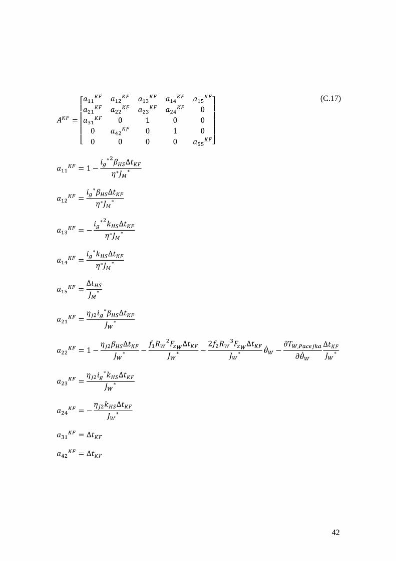
42

[

]

(C.17)

43

(

)

The Jacobian matrices and are identity matrices.

Appendix D – List of Notations

A: state matrix (for the state-space model formulation)

aij: element on the i-th row and j-th column of the state matrix

: Jacobian matrix of the partial derivatives of with respect to

: element on the i-th row and j-th column of the matrix

b: rear semi-wheelbase

44

B: input matrix (for the state-space model formulation)

C: output matrix (for the state-space model formulation)

Cd: aerodynamic drag coefficient

Cl: aerodynamic lift coefficient

Cm: aerodynamic pitch moment coefficient

D: feedthrough matrix (for the state-space model formulation)

dHS: half-shaft diameter

: Kalman Filter non linear difference equation of system state

fr: tyre rolling resistance coefficient

f0: part of the tyre rolling resistance coefficient independent from wheel tangential

velocity

f1: term of the tyre rolling resistance coefficient to be multiplied by wheel tangential

velocity

f2: term of the tyre rolling resistance coefficient to be multiplied by wheel tangential

velocity squared

Fz,W: vertical force between the wheel and the road

g: gravity

GCL,TC,conventional: closed-loop transfer function ref

σs

σof the vehicle with traction control

system based on direct slip control, without the feedback control of half-shaft torque

45

GLG: loop gain transfer function of the system

GPLANT: transfer function of the plant (the vehicle)

GPLANT,HS: transfer function of the plant (the vehicle), providing half-shaft torque as

output

GPLANT,σ: transfer function of the plant (the vehicle), providing slip ratio as output

: Jacobian matrix of the function with respect to

: Kalman Filter non-linear measurement equation

hCG: centre of gravity height

ig*: overall gear ratio of the single-speed transmission

ig1: gear ratio of the first stage of the single-speed transmission

ig2: gear ratio of the second stage of the single-speed transmission

ig3: gear ratio of the third stage of the single-speed transmission

JHS: mass moment of inertia of the half-shaft

JM: mass moment of inertia of the electric motor

*

MJ : mass moment of inertia of the electric powertrain at the motor

*

VJ : equivalent mass moment of inertia of the vehicle

JW: mass moment of inertia of a wheel

*

WJ : equivalent mass moment of inertia of a wheel

J1: mass moment of inertia of the transmission input shaft (Figure 1)

J2: mass moment of inertia of transmission shaft 2 (Figure 1)

46

J3: mass moment of inertia of transmission shaft 3 (Figure 1)

J4: mass moment of inertia of the transmission output shaft (Figure 1)

k: discretisation step parameter

K: Kalman gain

kHS: torsional stiffness of the half-shaft

KHS,CL: closed-loop transfer function of the half-shaft torque control system

KPID,TC: transfer function of the traction control system (PID controller)

L: vehicle wheelbase

lHS: half-shaft length

Ltyre: tyre relaxation length

m: vehicle mass

: error covariance matrix

PM,max: maximum motor power

: process noise covariance matrix

R: measurement noise covariance

RW: tyre radius

s: Laplace variable

S: frontal area of the vehicle (for aerodynamic force and moment computation)

Tdriver: driver torque demand (for the electric motor drive)

47

Td,W: delayed (due to tyre relaxation length effect) torque between tyre and road (with

time derivative ,d FWT )

THS: half-shaft torque

TM: electric motor torque (with time derivative MT )

TM,max: maximum electric motor torque

TM,ref: reference electric motor torque, according to driver input

*

,M refT : reference electric motor torque from the traction control (Figure 5)

**

,M refT : reference electric motor torque from the half-shaft torque control (Figure 5)

TW: net torque transmitted by the half-shaft to the driven wheel

Twindage: electric motor torque windage losses

TW,Pacejka: tyre torque according to the Pacejka magic formula model

U: input vector (for the state-space model formulation)

uW: longitudinal offset (due to the rolling resistance coefficient) between tyre normal

force and the centre of the contact patch

: measurement noise vector

: Jacobian matrix of the function with respect to

: process noise vector

: Jacobian matrix of with respect to

X: state vector (for the state-space model formulation)

48

Y: output vector (for the state-space model formulation)

: measurement vector

βHS: torsional damping coefficient of the half-shaft

: Kalman Filter time step

η*: overall efficiency of the single-speed transmission including the constant velocity

joint

ηj1: efficiency of the inner constant velocity joint

ηj2: efficiency of the outer constant velocity joint

η1: efficiency of the first stage of the single-speed transmission

η2: efficiency of the second stage of the single-speed transmission

η3: efficiency of the third stage of the single-speed transmission

, ,M M Mθ θ θ : angular displacement, velocity and acceleration of the electric motor shaft

,V Vθ θ : angular velocity and acceleration of the equivalent inertia of the vehicle

, ,W W Wθ θ θ : angular displacement, velocity and acceleration of a driven wheel

ρ: air density

σ: tyre slip ratio

σPEAK: tyre slip ratio at which the peak longitudinal force is achieved

σref: reference slip ratio

τM: electrical time constant of the electric motor drive

49

μ: tyre-road friction coefficient

In the frequency domain, the parameters have the same notation as in the time domain,

with a horizontal line at the top.

The subscript ‘0’ refers to the initial condition of a state variable.

The subscripts ‘F’ and ‘R’ refer to front and rear components of the vehicle.

The symbol ‘ ’ refers to the estimated variables.

The symbol ‘ ’ refers to the Laplace transform of a variable in the time domain.

The symbol ‘ ’ refers to a measured state.