The Effect of Grain Size Distribution on Nonlinear Flow ... · Transp Porous Med (2017) 120:37–66 DOI 10.1007/s11242-017-0903-3 The Effect of Grain Size Distribution on Nonlinear

Transp Porous Med (2017) 120:37–66DOI 10.1007/s11242-017-0903-3

The Effect of Grain Size Distribution on NonlinearFlow Behavior in Sandy Porous Media

Jan H. van Lopik1 · Roy Snoeijers1 · Teun C. G. W. van Dooren1 ·Amir Raoof1 · Ruud J. Schotting1

Received: 7 March 2017 / Accepted: 19 July 2017 / Published online: 24 August 2017© The Author(s) 2017. This article is an open access publication

Abstract The current study provides new experimental data on nonlinear flow behaviorin various uniformly graded granular materials (20 samples) ranging from medium sands(d50 > 0.39 mm) to gravel (d50 = 6.3 mm). Generally, theoretical equations relate theForchheimer parameters a and b to the porosity, as well as the characteristic pore length,which is assumed to be themedian grain size (d50) of the porousmedium.However, numericaland experimental studies show that flow resistance in porous media is largely determined bythe geometry of the pore structure. In this study, the effect of the grain size distribution wasanalyzed using subangular-subrounded sands and approximately equal compaction grades.We have used a reference dataset of 11 uniformly graded filter sands. Mixtures of filter sandswere used to obtain a slightly more well-graded composite sand (increased Cu values by afactor of 1.19 up to 2.32) with respect to its associated reference sand at equal median grainsize (d50) and porosity. For all composite sands, the observed flow resistance was higherthan in the corresponding reference sand at equal d50, resulting in increased a coefficientsby factors up to 1.68, as well as increased b coefficients by factors up to 1.44. A modifiedErgun relationship with Ergun constants of 139.1 for A and 2.2 for B, as well as the use ofdm − σ as characteristic pore length predicted the coefficients a and b accurately.

Keywords Forchheimer equation · Nonlinear flow · Filter sand · Grain size distribution ·Column experiment

1 Introduction

The understanding of nonlinear liquid or gas flow behavior in natural and artificial porousmedia, such as rock, consolidated or unconsolidated material and packed-bed-reactors is akey factor in reservoir engineering applications (Wen et al. 2011; Mijic et al. 2013; Yeh and

B Jan H. van [email protected]

1 Department of Earth Sciences, Environmental Hydrogeology group, Utrecht University,Princetonplein 9, 3584 CC Utrecht, The Netherlands

123

http://crossmark.crossref.org/dialog/?doi=10.1007/s11242-017-0903-3&domain=pdf

38 J. H. van Lopik et al.

Chang 2013; Houben 2015) and chemical and technical industries (e.g., Jafari et al. 2008).In the field of reservoir engineering, fluid flow behavior near the well screen controls theefficiency of oil/gas production wells (e.g., Holditz and Morse 1976; Aulisa et al. 2009),as well as the efficiency of injection/extraction wells in groundwater resources applications(e.g., Sen 1989; Mathias and Todman 2010; Wen et al. 2011, 2013; Yeh and Chang 2013;Houben 2015; Mathias and Moutsopoulos 2016). Moreover, nonlinear flow at full-aquiferscale in a broad range of geological formations, such as gravel, karstic or fractured aquifers,is widely addressed in the literature (e.g., Moutsopoulos and Tsihrintzis 2005; Moutsopoulos2007).

Commonly, groundwater flow near wells is described using the classical Darcy’s law(Darcy 1856), as:

i = − 1

Kq (1)

where i is the hydraulic gradient (m/m), K is the hydraulic conductivity of the porousmedium (m/s) and q is the specific discharge (m/s). This empirical linear relationship forfluid flow in porous media is only applicable for a specific regime of flow where flow veloc-ities are sufficiently low, and it becomes less accurate as flow velocities become larger.The deviation of the nonlinear relationship between specific discharge and hydraulic gradi-ent due to increased flow resistance at higher flow velocities has been widely addressed inthe literature (e.g., Forchheimer 1901; Izbash 1931; Sidiropoulou et al. 2007). Forchheimer(1901) described the nonlinear behavior adding a second-order quadratic term to the Darcy’slaw:

i = −aq − bq2 (2)

Comparing Eqs. 1 and 2, a (s/m) is a parameter equal to the reciprocal of the hydraulicconductivity (i.e., a = 1/K ) and b is the empirical Forchheimer coefficient (s2/m2). TheForchheimer equation is able to accurately fit the experimental data in packed-columnexperiments with granular material for most cases of non-Darcy flows (Sidiropoulou et al.2007; Moutsopoulos et al. 2009; Sedghi-Asl et al. 2014; Li et al. 2017). Mathias andMoutsopoulos (2016) showed that the Forchheimer equation should be used instead ofDarcy’s law to account for additional head losses due to non-Darcy flow conditions in thevicinity of injection and production wells. Other analytical studies use the Forchheimerequation to predict non-steady-state, nonlinear flow in gravel aquifers at early time stepswhen hydraulic gradients are steep (e.g., Moutsopoulos and Tsihrintzis 2005; Moutsopoulos2007).

Besides the Forchheimer equation, other empirical equations have been proposed todescribe the relation between specific discharge and hydraulic gradient for nonlinear flow(Izbash 1931; Irmay 1958; Bear 1972). For example, the Izbash equation’[initially proposedby Forchheimer (1901)], which is a nonlinear power law function, is widely used to modelthe non-Darcy flow (e.g., Bordier and Zimmer 2000; Wen et al. 2013). Despite the exper-imental validity of the Izbash equation, it lacks any physical base (Bordier and Zimmer2000).

Many experimental data on (post-Darcy) nonlinear flow in porous media are availablefor coarser porous media, such as coarse sands, gravels and glass beads (Sidiropoulouet al. 2007; Moutsopoulos et al. 2009; Sedghi-Asl and Rahimi 2011; Huang et al. 2013;Bagci et al. 2014; Salahi et al. (2015); Sedghi-Asl et al. 2014; Li et al. 2017). A rel-atively small amount of experimental data is available for finer unconsolidated sandyporous media. Moreover, most studies only provided porosity and the median (d50) or

123

The Effect of Grain Size Distribution on Nonlinear Flow… 39

mean grain size to describe the porous media. Relationships to predict Forchheimer coef-ficients a and b are based on these two parameters (e.g., Ergun 1952; Macdonald et al.1979; Kovács 1981; Kadlec and Knight 1996; Sidiropoulou et al. 2007). However, numer-ical simulations, as well as experimental studies, showed that the geometry of the porestructure have a large influence on flow behavior (e.g., Hill and Koch 2002; Li and Ma2011; Allen et al. 2013; Koekemoer and Luckos 2015). Here, we investigated the effectof nonlinear flow behavior empirically for granular porous media (filter sand) with vari-ous grain size distributions for a given reference median grain size (d50) and compactiongrade.

2 Background

2.1 Criteria for Nonlinear Flow in Porous Media

Experimental and numerical studies have investigated the upper limits of the Darcy regimefor fluid flow in porous media. Many attempts have been done to define a criterion to describethe upper limit of the Darcy regime. Formerly, it was believed that nonlinear flow behaviorin porous media was solely due to turbulent flow (inertial energy losses by highly chaoticand unsteady flow).

The Reynolds number is used to indicate whether fluid flow is laminar or turbulent. It isdefined as (Bear 1972):

Re = ρd50q

μ= inertial forces

viscous forces(3)

where ρ is the fluid density (kg/m3), d50 is the median grain size of the porous medium asa proxy for the characteristic pore length (m), q is the specific discharge (m/s), and μ is thedynamic viscosity (kg/m s). Besides Reynolds number, which is solely based on the averageparticle size of the porous medium to define the properties of the medium, various othercriterions have been proposed. For example, Ergun (1952) used a modified Reynolds numberby including porosity, while Comiti et al. (2000) used a pore Reynolds number based onporosity, tortuosity and the dynamic specific surface area of the pore. Zhengwen and Grigg(2006) stated that determination of a representative pore diameter as characteristic lengthof the porous media is difficult, due to the complexity of pore structures. Moreover, flowthrough a complex pore structure significantly differs from flow in a conduit, and, hence, nosharp transition between laminar and turbulent flow can be observed in porous media. A widerange of critical particle Reynolds numbers is given in the literature for the onset of nonlinearlaminar flow. For example, Bear (1972), Hassanizadeh and Gray (1987), Ma and Ruth (1993)and Comiti et al. (2000) suggested critical particle Reynolds numbers ranging between 1 and15. Other studies, such as Scheidegger (1974), obtained higher maximal critical particleReynolds numbers up to a value of 75.

Ma and Ruth (1993) and Lage (1998) introduced new criteria to evaluate the onset ofnonlinear flow by means of a “Forchheimer number,” based on the intrinsic permeabilityand the non-Darcy coefficient b in the Forchheimer equation. However, such criteria requireexperimentally or empirically determined values for the Forchheimer coefficients a and b,while criteria such as the particle Reynolds number require only the average grain size inorder to estimate the onset of nonlinear flow in a given porous media.

123


2.2 Nonlinear Laminar Flow and Fully Turbulent Flow in Porous Media

Traditionally, it was believed that the onset of nonlinear flow was solely due to energy lossesby the occurrence of turbulence (e.g., Ergun 1952; Ward 1964). However, flow visualizationstudies in porous media showed that turbulent flow occurs at much higher particle Reynoldnumbers than the critical particle Reynold numbers of 1–15 for the onset of nonlinear flow(e.g., Chauveteau and Thirriot 1967; Dybbs and Edwards 1984; Seguin et al. 1998). Criticalparticle Reynolds number of 300–533 was determined for the onset of the turbulent flowregime using a uniform spheres packing with particle diameters ranging from 0.5 to 8 cm,respectively (Jolls and Hanratty 1966; Latifi et al. 1989; Rode et al. 1994; Seguin et al.1998), as well as for cylindrical or plate arrangements (Dybbs and Edwards 1984). Hence,a nonlinear laminar flow regime should be considered before fully turbulent flow developsin porous medium. A smooth transition was observed from nonlinear laminar flow, to theonset of small vortices and eddies in some pore spaces, to eventually, development of fullyturbulent flow in the porous medium (e.g., Dybbs and Edwards 1984; Seguin et al. 1998). Inthe literature, this nonlinearity in the laminar flow regime is ascribed to different microscaleprocesses (e.g., Hassanizadeh and Gray 1987; Ma and Ruth 1993; Skjetne and Auriault1999; Hill and Koch 2002; Nield 2002). In general, it is assumed that the deviation from thelinear Darcy’s law at increased Reynolds numbers is due to the occurrence of microscopicinertial forces (e.g., Bear 1972; Macdonald et al. 1979; Venkataraman and Rao 1998). Otherstudies, such as Panfilov et al. (2003) and Panfilov and Fourar (2006), showed that the mainmechanisms of energy dissipation that contribute to the nonlinear flow term are due to bothrecirculation of eddies in closed streamline regions, as well as streamline deformation in themain area of flow. Ma and Ruth (1993) showed that the onset of nonlinearity cannot be fullydescribed by microscopic inertial terms using a simple tube model. Hassanizadeh and Gray(1987) stated that the onset of nonlinear flow behavior is due to the occurrence of interfacialdrag forces at increased flow velocities and inertial forces become significantly important atparticle Reynold numbers of about 100. The effect of the viscous boundary layer on dragwas addressed by Whitaker (1996). These studies showed that microscopic analysis shouldbe used to fully understand macroscopic nonlinear laminar flow behavior in a given complexpore structure for a given Reynolds number. Overall, the geometry of the pore structure(such as tube-like or blob-like pore surfaces), as well as the total fluid–solid interface andits interface roughness, largely determine the flow resistance due to drag force terms in theForchheimer coefficient b (e.g., Ma and Ruth 1993; Liu et al. 1995; Thauvin and Mohanty1998; Panfilov and Fourar 2006; Chaudhary et al. 2013).

As described above, themacroscopic transition from laminarDarcy flow, to nonlinear lam-inar flow to eventually fully turbulent flow, is a gradual process (e.g., Seguin et al. 1998).Manyexperimental datasets on nonlinear flow behavior in granular porous media show that thisgradual process can be accurately predicted by the Forchheimer equation (Eq. 2) for variousranges of particle Reynold numbers in the nonlinear laminar flow regime, as well as in the tur-bulent flow regime (e.g., Venkataraman and Rao 1998; Sidiropoulou et al. 2007; Moutsopou-los et al. 2009; Bagci et al. 2014; Sedghi-Asl et al. 2014; Salahi et al. 2015; Li et al. 2017).

For example, Li et al. (2017) conducted flow experiments on sands at Reynolds numbersbelow 40 and, hence, investigated the onset of the nonlinear laminar regime. By contrast,Sedghi-Asl et al. (2014) investigated the Forchheimer coefficients of sands and gravel exper-imentally at Reynold numbers ranging from 31 to 720 (for a sand with d50 of 5.5 mm) upto 2400–30,750 (for a gravel with d50 of 56.8 mm). Moutsopoulos et al. (2009) evaluatedcoefficients a and b for different granular materials, ranging from sand, gravel, carbonaterocks up to cobbles (with d50 ranging from 2.71 to 67.2 mm). In the experimental study

123


of Salahi et al. (2015), rounded and crushed angular grains (with d50 ranging from 1.77 to17.78 mm) were used. The maximum Reynolds numbers used in these studies are 437–2709(Moutsopoulos et al. 2009) and 714–1882 (Salahi et al. 2015).

It should be noted that the experiments for analyzing the onset of turbulence for flow inporous media (e.g., Seguin et al. 1998) are performed on spheres with one single diameter.However, natural granular materials have different grain size distributions, gradations andshape irregularities. The difference in pore structure and particle roughness could result indifferent Reynolds numbers for the onset of turbulent flow, and the critical Reynolds numbersfor turbulence might significantly differ from 300 to 533. Andersen and Burcharth (1995)stated that for such materials the transition zones between the different flow regimes areblurred and difficult to define. This might explain that a reasonable singular fit with theForchheimer equation (Eq. 2) is obtained for flow experiments on sand and gravel for awide range of Reynold numbers (e.g., Moutsopoulos et al. 2009; Sedghi-Asl et al. 2014).Similar conclusions can be obtained from numerical studies, such as Firdaouss et al. (1997)and Fourar et al. (2004), which consider the Forchheimer equation (Eq. 2) valid over a widerange of Reynolds numbers.

Some studies have tried to characterize the nonlinear flow regime in terms of aweak inertialand strong inertial regime (fully turbulent flow regime) based onmacroscale flow experimentsin packed spheres of uniform size and determined different Forchheimer coefficients for bothregimes (e.g., Fand et al. 1987; Bagci et al. 2014). The extent of these regimes was estimatedfrom the reduced pressure drop versus flow velocity. Bagci et al. (2014) defined a turbulentflow regime for critical particle Reynolds numbers >268, while Fand et al. (1987) obtainedRe values >120.

2.3 Empirical Relations for Estimation of the Forchheimer Coefficients

In many cases, the hydraulic characteristics by means of the Forchheimer coefficients a andb for a given porous medium sample are not available. Empirical relations can be used topredict the Forchheimer coefficients by using the soil characteristics, such as the averagegrain size and porosity. Many studies have developed empirical relations for the coefficientsa and b (see Eq. 2). An overview of these expressions is given in Table 1.

Schneebeli (1955) proposed expressions for coefficients a and b for porous media con-sisting of spheres. The average particle diameter (d) is used as characteristic pore lengthof the porous medium. Ward (1964) proposed similar expressions based on nonlinear flowexperiments with 20 different porous media consisting of material ranging from glass beadsto sand and gravel, having particle diameters of 0.27–16.1 mm.

Based on the Kozeny–Carman relationship for Darcy flow (Carman 1937), Ergun (1952)derived an expression for the b coefficient. The assumption of Ergun’s (1952) approach isthat fluid flow in porous media is similar to flow in pipes, assuming full turbulent flow inthe nonlinear flow regime (Ergun 1952; Lage 1998). However, as described above, nonlinearflow at intermediate Reynolds numbers is laminar. Nevertheless, Ergun’s (1952) relationswork quite well for nonlinear flows in various kind of porous media and are, to a great extent,the most analyzed and used relationships (e.g., Sidiropoulou et al. 2007; Li and Ma 2011;Allen et al. 2013; Bagci et al. 2014). Many variations on the Ergun relations for differentkind of porous media with a wide range of Ergun constants A and B are addressed in theliterature (e.g., Macdonald et al. 1979; Fand et al. 1987; Comiti and Renaud 1989). Kovács(1981) analyzed a dataset of 300 sediment samples for Re = 10−100 and proposed a valueof 144 for constant A and 2.4 for constant B. Du Plessis (1994) investigated the increasein flow resistance due to local flow recirculation in the pore spaces in the nonlinear laminar

123


Table 1 Empirical relations for the Forchheimer coefficients a and b

Equations Coefficient a (s/m) Coefficient b (s2/m2)

Schneebeli (1955) (4) 1100 v

gd212 1

gd

Ward (1964) (5) 360 v

gd210.44 1

gd

Ergun-type (6) A (1−n)2vgn3d2

B (1−n)

gn3d

Carman (1937) A = 180 –

Ergun (1952) A = 150 B = 1.75

Kovács (1981) A = 144 B = 2.4

Macdonald et al. (1979) (7) 180 (1−n)2vgn3.6d2

1.8 (1−n)

gn3.6d

Kadlec and Knight (1996) (8) 255 (1−n)v

gn3.7d22 (1−n)

gn3d

Sidiropoulou et al. (2007) (9) 0.0033 d−1.50n0.0603 0.194 d−1.27n−1.14

Geertsma (1974) (10) –(0.005g (k 10000)−0.5n−5.5

)

Where g is the acceleration due to gravity (m/s2), v is the kinematic viscosity (m2/s), d is the characteristicpore length bymeans of an average particle diameter (m), n is the porosity (−), and k(= μ/ρga) is the intrinsicpermeability (m2)

flow regime. From these analytical results, it was concluded that in the laminar flow regimethe Ergun constants were higher than derived by Ergun (1952) for turbulent flow in porousmedia. Both constants are functions of porosity, where constant A increases with increasingporosity, and constant B decreases with increasing porosity. For porousmedia with a porosityranging between 0.33 and 0.36, constant A is approximately 200, while constant B is 1.97.Engelund (1953) derived a similar expression as Ergun (1952) for Forchheimer coefficient band stated that the constant B varies from a value of 1.8 for uniform spherical particles, upto a value of 3.8 for highly irregular angular grains.

Macdonald et al. (1979) and Kadlec and Knight (1996) suggested different forms of theErgun relation by changing the porosity term (1 − n)2/n3 and (1 − n)/n3 for, respectively,coefficient a and coefficient b (see Table 1). Macdonald et al. (1979) used analyzed exper-imental datasets which included a wide variety of porous media (e.g., glass beads, steelspheres (blue metal), cylindrical fibers and granular material) with porosities ranging from0.123 to 0.919. For Eq. 7b ofMacdonald et al. (1979), the constant 1.8 works well for smoothparticles (see Table 1), while for rough particles a value of 4.0 is preferred for estimatingthe coefficient b. For intermediate surface roughness of the particles, the value should liebetween these two values.

Sidiropoulou et al. (2007) derived empirical relationships, which are based on linearregression analysis on both porosity and the average particle size for a large dataset fromthe literature. Geertsma (1974) derived an empirical relationship for estimating Forchheimercoefficient b based on intrinsic permeability, k, and porosity, examining an experimentaldataset of consolidated and unconsolidated sandy porous media.

Many studies are using the median particle diameter (d50) as the characteristic lengthfor the pore space. However, Macdonald et al. (1979) suggested that the use of the surface-volume mean diameter dSm (also referred to as Sauter mean diameter) as a more appropriatecharacteristic length compared to the d50. It is defined as the diameter of a sphere that hasthe same volume/surface area ratio as the particle of interest. For a perfect spherical particle,the surface area moment mean diameter dSm equals:

123


dSm = 6Vp

sp= d32 (11)

where Vp/sp is the ratio between volume and surface area of the sphere. Note that for non-spherical particles, as well as an rougher particles this ratio decreases and, hence, the averagecharacteristic pore length of the porous medium decreases (Allen et al. 2013; Li and Ma2011; Macdonald et al. 1979). In general, it is challenging to determine the exact surface areaof natural porous materials.

2.3.1 Evaluation of the Empirical Relations on Experimental Datasets of GranularMaterial

Several studies have analyzed the theoretical and empirical relationships in Table 1 for Forch-heimer coefficients a and b. Sedghi-Asl et al. (2014) predicted the experimentally derivedcoefficients a and b accurately using Sidiropoulou et al. (2007) for sands with d50 rangingfrom 2.83 to 56.8 mm. A reasonable prediction for coefficient a was obtained using Ergun(1952) and Kovács (1981). However, coefficient b was systematically overestimated usingKovács (1981).

Moutsopoulos et al. (2009) predicted the experimentally derived coefficients a and baccurately using Kovács (1981) for sands with a d50 of 2.71–67.23 mm. The equation byWard (1964) significantly underestimated the coefficients a and b. The equation by Kadlecand Knight (1996) significantly overestimated coefficient a, but a good fit was obtained forthe coefficient b. Moreover, Moutsopoulos et al. (2009) also suggested the use of d20 andd30 as particle diameter for the equation by Ward (1964), to provide good predictions forcoefficients a and b.

Sidiropoulou et al. (2007) investigated a large dataset collected from the literature. Forcoefficient a, the equation by Ward (1964) significantly underestimated the experimentallyderived coefficient, while the equation by Kadlec and Knight (1996) resulted in significantoverestimation of the coefficient. Only the equation by Ergun (1952), resulted in a reasonablefit for coefficients a and b, where overall a underestimation was obtained for the experimen-tally derived coefficient. The equation byWard (1964) resulted in significant underestimationof the values. Due to the relative poor fits, Sidiropoulou et al. (2007) suggested to use analternative equation for accurate estimation of the Forchheimer coefficients (see Table 1).Salahi et al. (2015) also suggest the use of the equation proposed by Sidiropoulou et al. (2007)to obtain the best estimates for Forchheimer coefficients a and b for their dataset.

The purpose of the current study is to compare the expressions in Table 1 with our exper-imental dataset on filter sands and the experimental datasets in the literature.

2.4 Friction Factor and Reynolds Number

In the literature, many forms of the Darcy–Weisbach equation, which was initially derivedfor analyzing flow resistance in a conduit, are suggested for flow in porous media (e.g.,Ergun 1952; Stephenson 1979; Herrera and Felton 1991). The method of Stephenson (1979)is widely used (e.g., Sedghi-Asl and Rahimi 2011; Salahi et al. 2015):

f = 2igdn2

q2and Res = ρd50q

nμ(12)

The relation between Reynolds number Res and the friction factor f is usually given by:

f = asRes

+ bs (13)

123


where as and bs are dimensionless variables. Herrera and Felton (1991) used the mean grainsize and standard deviation of the grains size distribution of a given sand type (dm − σ ) ascharacteristic pore length in Darcy–Weisbach and Reynolds number equations (Eqs. 12, 13).They stated that for well-graded material with large standard deviations, finer particles fillthe pores between coarser particles and the contact surface of particles with water increases.For such conditions, the flow resistance increases resulting in decreased flow velocity andReynolds number. We have tested both the method of Stephenson (1979) with ReS andHerrera and Felton (1991) with ReH .

3 Methods

3.1 Experimental Setup

In order to measure one-dimensional flow in various sandy porous media, we used the exper-imental setup as shown in Fig. 1. It consists of the following main components; (1) the inlet,(2) the column with sandy porous medium, (3) the outlet and (4) the circulation tank of 1 m3

with a pump. A Plexiglas sample column (2) with a length of 0.507 m, a wall thickness of0.5 cm and an inner diameter of 9.8 cm contained the sandy porous media. The investigatedsandy porous media have median grain sizes (d50) of 0.39–2.11 mm that are a factor 0.0040and 0.0215 smaller than the diameter of the column, while for gravel (d50 of 6.34 mm) thefactor was 0.065 smaller. Fand and Thinakaran (1990) stated that the ratio between d50 andcolumn diameter should be lower than 0.025, to ensure that the flow parameters are substan-tially independent of the wall effects of the column. The highest ratio in the literature forconducted flow experiments was in the same range (0.032 for Li et al. 2017, 0.089 for Salahiet al. 2015, 0.13 for Moutsopoulos et al. 2009 and 0.19 for Sedghi-Asl et al. 2014). The waterpressure in the columnwasmeasured at a distance of 0.13, 0.26 and 0.38m from the inlet. Thepressure at the inlet compartment (1) was also measured, while at the outlet compartment (3)the hydraulic head was fixed at 0.505 m. For all experiments, a linear hydraulic head gradientwas obtained by interpolation of the measured water heads at the pressure monitoring points(5). The water pressure was measured with a BD Sensors pressure transmitter combined witha BD Sensors PA 430 display (5). The volumetric flow rate Q (m3/h) was measured using aMetrima SVM F2 Energy Meter (6), which was placed between the pump (4) and the inletcompartment (1).

For each experiment on a single sand sample, the flow rate was determined for varioushydraulic gradients, i(= (h1 − h2)/L), by using different injection pressures. The pressuresranged from 0.1 to 3.2 bar (15 different injection pressures) for the finest granular material(S.1) and ranged from 0.1 to 1.2 bar (12 different injection pressures) for the coarsest granularmaterial (S.11). At a given hydraulic gradient, the flow rate was determined for at least morethan 29 times to ensure achievement of steady state flow conditions (defined as<3%variationin flow) in the porous medium. The temperature was measured in the outlet section of theexperimental setup. To ensure constant water density and viscosity, the temperature in thecirculation tank was kept constant at 20 ◦C (±0.3 ◦C).

We have used the particle Reynolds number (Eq. 3) to determine the upper limit of theDarcy regime. For analysis, a deviation fromDarcy’s law is considered by observing a relativedifference of 5%between the actual specific discharge described by the Forchheimer equation(Eq. 2) and the specific discharge described by Darcy’s law (Eq. 1). The critical Reynoldsnumbers (Recr ) are obtained for all investigated sandy porous media.

123


Fig. 1 Schematic overview of the experimental setup: 1 inlet compartment, 2 column with packed sandyporous medium, 3 outlet compartment, 4 circulating tank with pump, 5 pressure sensor and 6 volumetric flowmeter

3.2 Description of the Investigated Sandy Porous Media

In this study, two sets of sandy porous media were investigated:

– At first, 11 uniformly graded filter sands (delivered by FILCOMcompany at Papendrecht,the Netherlands) with various median grain sizes (d50) were used as reference porousmedia to obtain the Forchheimer coefficients a and bexperimentally (Samples 1–11).These filter sands are used as gravel pack around well screens to increase well efficiency,and also for packed sand beds for drinking water or wastewater treatment.

– Subsequently, these filter sands were mixed to obtain 9 different packed sandy porousmedia with wider grain size distributions at a given median grain size (d50) that equalsone of the reference filter sands (Samples 3–8). Hence, we were able to test the effectof various grain size distributions for a given median grain size (d50) on nonlinear flowbehavior experimentally (Samples 3.1, 4.1, 5.1 6.1–4, 7.1 and 8.1).

The porosity of each packed sample was determined by weighing the dry mass granular sandor gravel in the column. The solid-phase density of the sand and gravel equals 2.66 kg/m3

(data by FILCOM).The granulometric sieve data for the 11 reference sands were used to analyze the grain

size distributions. The median grain size (d50), and the grain sizes d10, d30 and d60 are listedin Table 2. The arithmetic method of moments was used to determine the mean particlediameter (dm) and the standard deviation (σ ) from the normal grain size distribution of thefilter sands (Blott and Pye 2001), yielding

dm =∑N

i=1 fi di100

(14)

123


Table 2 The grain size distribution characterization for uniformly graded filter sands used as reference

Sample d50(mm)

d10(mm)

d30(mm)

d60(mm)

dm(mm)

σ

(mm)dm − σ

(mm)CC CU n (−)

1 0.39 0.29 0.35 0.41 0.39 0.0845 0.31 1.05 1.39 0.344

2 0.39 0.28 0.34 0.41 0.39 0.0852 0.30 1.04 1.48 0.335

3 0.61 0.47 0.55 0.64 0.61 0.112 0.50 0.99 1.37 0.331

4 0.71 0.53 0.63 0.76 0.72 0.155 0.57 0.99 1.42 0.340

5 0.84 0.72 0.80 0.86 0.84 0.0921 0.75 1.02 1.19 0.333

6 0.99 0.80 0.91 1.03 0.98 0.164 0.82 1.01 1.30 0.346

7 1.05 0.89 0.98 1.08 1.05 0.138 0.91 1.00 1.21 0.348

8 1.36 1.13 1.27 1.41 1.35 0.189 1.16 1.01 1.25 0.358

9 1.50 1.16 1.34 1.58 1.52 0.287 1.23 0.98 1.36 0.358

10 2.11 1.72 1.97 2.18 2.07 0.306 1.76 1.03 1.27 0.357

11 6.34 5.16 5.87 6.55 6.28 0.938 5.34 1.02 1.27 0.361

and

σ =√∑N

i=1 f (di − dm)2

100, (15)

where N is the number of used sieves for the grain size analysis, f is the passing frequencyin percent on the corresponding i th sieve, and di (mm) is the average grain size diameter ofthe i th sieve class interval. For the composite sands, specific portions of the reference sandswere mixed. From the reference sand fractions, a new grain size distribution was determinedand the dm and σ were calculated based on a number of equal step intervals (N ) subdividingthis grain size distribution. For non-uniformly graded granular material, Herrera and Felton(1991) used the standard deviation of particle sizes and substituted the characteristic porelength d by dm − σ .

Moreover, the coefficient of uniformity Cu (−) and the coefficient of curvature Cc (−) ofthe grain size distribution are calculated, using

CU = d60d10

(16)

and

CC = (d30)2

d10d60(17)

In line with the study of Moutsopoulos et al. (2009), we used the values d10, d30 and d50 ascharacteristic pore length, d , in the empirical equations listed in Table 1. Also the method ofHerrera and Felton (1991) was used by considering dm − σ as the characteristic pore length.

3.2.1 Reference Sands

The filter sands used in this study are classified as medium sand (S.1–2), coarse sand (S.3–6),very coarse sand (S.7–10) and fine gravel (S.11) (Blott and Pye 2001). The reference filtersands are uniformly graded with a Cu < 1.48, Cc ranging from 0.98 to 1.05, and smallarithmetic standard deviations (σ <0.938 mm) for all 11 samples (Table 2). All filter sandshave a normal grain size distribution, resulting in approximately equal median grain sizes

123


Table 3 The grain size distribution characterization for the filter sand mixtures

Sample d50(mm)

d10(mm)

d30(mm)

d60(mm)

dm(mm)

σ

(mm)dm − σ

(mm)CC CU n (−)

3.1 0.62 0.40 0.53 0.66 0.62 0.168 0.45 1.06 1.63 0.334

4.1 0.71 0.44 0.60 0.77 0.72 0.218 0.50 1.04 1.74 0.332

5.1 0.84 0.57 0.73 0.89 0.84 0.203 0.64 1.06 1.56 0.337

6.1 0.99 0.61 0.85 1.08 1.03 0.350 0.68 1.10 1.78 0.330

6.2 0.99 0.68 0.89 1.03 0.96 0.208 0.75 1.12 1.52 0.344

6.3 0.99 0.74 0.89 1.05 1.01 0.240 0.77 1.01 1.42 0.348

6.4 1.01 0.53 0.74 1.23 – – – 0.84 2.32 0.332

7.1 1.06 0.71 0.91 1.12 1.07 0.311 0.76 1.06 1.58 0.337

8.1 1.36 0.81 1.12 1,49 1.39 0.453 0.93 1.03 1.84 0.345

(d50) and mean grain sizes (dm). The roundness of the granular material is classified assubangular-subrounded.

3.2.2 Composite Sands

Table 3 and Fig. 9 show that the d50 of the composite sands is equal to its correspondingreference sand. The composite sands (S.3.1–8.1) are slightly more well graded resulting inincreased Cu values by a factor of 1.19 up to 1.47, while Cc values are more or less equalto the reference sands. The wider grains size distribution is also reflected by the increasedstandard deviation values. All composite sand samples have a normal grain size distribution,except for Sample 6.4. For that case, a bimodal grain size distribution was obtained, withpeaks at 0.75 and 1.38 mm. Hence, a reduced Cc value of 0.84 and an increased Cu value of2.32 are obtained.

The use of slightly more well-graded sands results in approximately equal porosities forboth the reference and composite sands (with a relative errors ranging between 0.6 and 4.8%).Much wider grains size distributions are required to obtain significant reduction of porosityat a given median grain size (d50). Only for the gap-graded composite sand S.6.4 with aclear bimodal grain size distribution, and for the more well-graded sand S.6.1 slightly lowerporosity values of, respectively, 0.330 and 0.332 were obtained with respect to the referencesand S.6 (n = 0.345).

3.3 Preparation Technique for the Sandy Porous Media

A consistent and reproducible packing method for the column samples was used to obtainhomogenously packed porous media. Different compaction preparation techniques weretested, to obtain the highest grain density and, hence, optimal compaction grades for eachsample column. We followed the method by Rietdijk et al. (2010) by using a constant plu-viation rate of the sand, as well a continuous manual compression of the deposited sand ina fully saturated column. This resulted in the lowest porosity values for the packed porousmedia samples, ranging from 0.33 for uniformly graded medium sand (Sample 1) to 0.36for uniformly graded gravel (Sample 11) (Table 2). Other packing methods resulted in sig-nificantly higher porosities (up to 0.38–0.40) of the porous medium. The lower compaction

123


grades resulted in non-rigid pore structures at increased fluid pore pressures in the columnduring the flow experiment tests.

Repeatedly testing of the Rietdijk et al. (2010) method as sample preparation techniquefor a given filter sand showed that a reproducible compaction grade, and hence porosity (rel-ative errors ranging between 0.02 and 1.1%) was obtained. For flow behavior, the maximalrelative error for coefficient a was 2.0% and for coefficient b 3.1%. The reproducibilitywas tested for the reference filter sands S.2, S.3 and S.5. Therefore, we have used theRietdijk et al. (2010) method for each sample to obtain an equal compaction grade andporosity over the entire column length and to ensure a stable pore structure of the sandyporous medium during the flow behavior experiments at increased injection pressures (up to3 bar).

After the saturated sample preparation of the sample column inside a container filledwith water, the inlet and outlet compartments were mounted under water to ensure no airinclusion occurred during the whole procedure. The water head at the inlet and outlet sideprovided fully saturated conditions during the installation into the experimental setup withthe measuring equipment.

3.4 Validity Analysis of the Empirical Relationships for Predicting ForchheimerCoefficients

The experimental dataset from this study was used to analyze the validity of the empiricalrelationships listed in Table 1. In order to compare the experimentally derived coefficients aand b, with the empirically predicted coefficients by Eqs. 4–10, the following methods areused; (1) the normalized objective function (NOF) criterion and (2) linear regression analysis.A similar approach was used in the studies of Moutsopoulos et al. (2009), Sedghi-Asl et al.(2014) and Sidiropoulou et al. (2007). Hence, a comparison can be made between our resultsand the results of their studies.

The NOF is defined as the ratio between the root mean square error (RMSE) to the overallmean value X of the experimental data.

NOF = RMSE

X, (18)

where:

RMSE =√∑N

i=1 (xi − yi )2

N(19)

and

X = 1

N

N∑i=1

xi (20)

Here xi are the experimental values for either the a coefficients or the b coefficients of theForchheimer equation (Eq. 2) and yi the corresponding values computed by the empiricalrelationship (Eqs. 4–10) for which the NOF analysis is done. A NOF value lower than 1.0implies a reasonable prediction of the coefficients a and b by the empirical relationships,where values close to 0.0 implies a perfect fit.

Linear regression is applied on scatter plots with the experimentally derived Forchheimercoefficient on the horizontal axis and the empirically predicted coefficient by the relationship(Eqs. 4–10) on the vertical axis. For a good prediction, the slope of the regression line equals1.0. Values that are lower than 1.0, imply underestimation of the Forchheimer coefficientsby the empirical relationship, while values higher than 1.0 imply overestimation. Moreover,

123


the R2-coefficient should be close to a value of 1.0 to ensure reduced scattering of the datapoints along the regression line.

4 Results

In this section, first, the reference experimental dataset on nonlinear flow behavior in the11 samples of filter sands is presented. Subsequently, the nonlinear flow behavior in thecomposite sands is presented and compared to the reference dataset. Moreover, a comparisonbetween the whole dataset of this study and the experimental data of existing literature isgiven. Finally, the empirical relationships for estimating the Forchheimer coefficients a andb in Table 1 (Eqs. 4–10) are verified using our experimental dataset.

4.1 Nonlinear Flow Behavior in the Reference Sands

Using the Forchheimer relation for nonlinear flow (Eq. 2) between the hydraulic gradient i andthe specific discharge q , the Forchheimer coefficients a and b are determined. Figure 2 showsthe Forchheimer fits on the experimental data for all 11 reference sands. For all investigatedsamples, the nonlinear flow behavior could be accurately described using the Forchheimerrelation, resulting in R2-coefficients >0.99 (see Table 4). The linear Darcy flow i = aq isalso plotted (dashed line) to show the nonlinear deviation from Darcy’s law at increased flowvelocities. Table 4 shows that only Samples 1–4 have a critical Reynolds number Recr for theonset of nonlinear flow within the measured range Remin − Remax. The rest of the sampleshave only data in the nonlinear flow regime.

The critical Reynolds numbers in this study vary between 2.21 and 4.13 (see Table 4),which fall in the limits of 1–15 reported in the literature (e.g., Bear 1972; Hassanizadeh andGray 1987; Comiti et al. 2000).

For the reference sands S.1 and 2, multiple data points were in the Darcy regime and,hence, the coefficient a can be determined directly using a linear interpolation (i = aDarcyq).For Sample 1, coefficient aDarcy is 1962.5 with R2 > 0.99 (5 data points), while for Sample 2,aDarcy is 1453.5 with R2 = 0.99 (4 data points). The aDarcy coefficients are in agreement withthe a coefficients determined by the Forchheimer fit over the whole dataset (see Table 4),resulting in small relative errors of 2.1 and 1.9%, respectively. This is in agreement withthe results of Venkataraman and Rao (1998), who also observed similar coefficients forForchheimer a and aDarcy. However, other studies showed that the Forchheimer coefficienta in the nonlinear flow regime can significantly differ from the resistance coefficient aDarcyin the Darcy regime (see Bagci et al. 2014).

Note that the coefficient a for S.2 is significantly lower than for S.1, while the grain sizedistribution and porosity of both filter sands are more or less identical. The decreased flowresistance for S.2might be due to a significant difference in the geometry of the pore structure.However, such differences in geometry should be due to large contrast in particle roughnessor grain shape, which is unlikely in our case with subangular-subrounded grains of the filtersands.

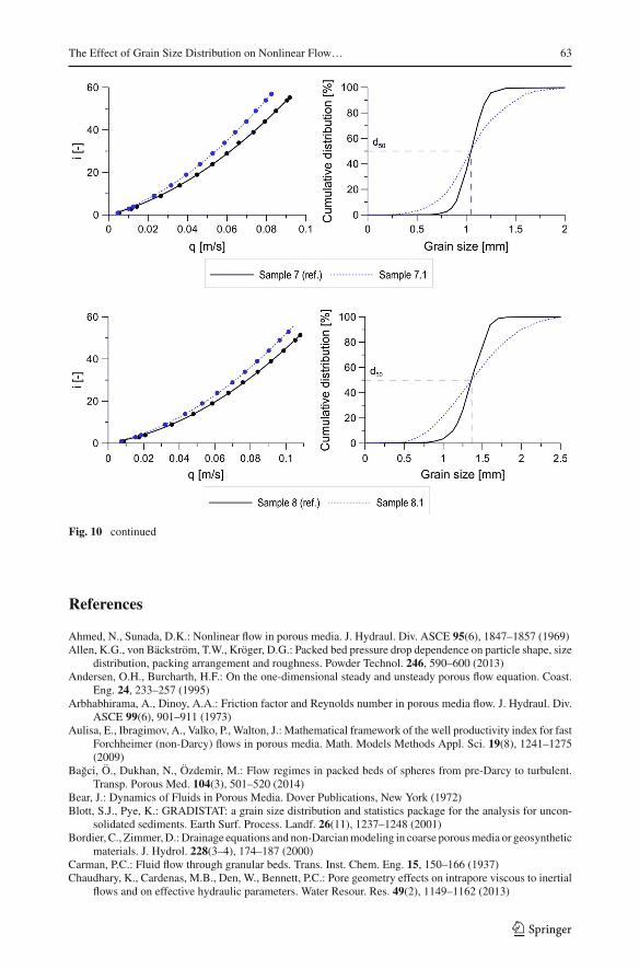
4.2 Nonlinear Flow Behavior in the Composite Sands

Similar to the reference sands, the nonlinear flow behavior for the composite sands couldbe described accurately by the Forchheimer equation (Eq. 2). The R2-coefficients are largerthan 0.99 for all plots (see Table 5). Figure 10 shows that for the slightly more well-graded

123


Fig. 2 The i − q plots for the sandy reference porous media S1–11. The linear Darcy flow i = aq is plotted(dashed line) to visualize nonlinear deviation from Darcy’s law

123


Fig. 2 continued

Table 4 The Forchheimer coefficients a and b for the reference sands (S.1–11)

Sample d50 (mm) Remin Remax Recr a (sm−1) b (s2m−2) R2

1 0.39 0.26 10.72 2.76 1,921.3 13,541 >0.99

2 0.39 0.33 13.02 2.21 1,426.5 12,523 >0.99

3 0.61 1.21 34.59 2.67 696.96 7,007.6 >0.99

4 0.71 1.58 43.72 2.96 562.16 6,781.8 >0.99

5 0.84 3.28 62.07 2.69 358.56 5,641.1 >0.99

6 0.99 5.02 87.29 2.76 245.75 4,396.0 >0.99

7 1.05 5.51 96.28 3.34 247.23 3,881.2 >0.99

8 1.36 11.78 147.06 3.08 140.60 3,104.0 >0.99

9 1.50 16.33 179.44 3.16 104.98 2,497.9 >0.99

10 2.11 29.65 287.92 3.90 64.503 1,746.3 >0.99

11 6.34 248.34 1196.78 4.13 7.9551 610.88 >0.99

composite sands the flow resistance was increased due to an increase in the fraction of smallerparticles (decreased d10 and d30 and increased Cu values) with respect to the reference sandsat equal median grain size (d50) (see Table 3; Figs. 3, 10). This means that the a coefficientswere increased by factors up to 1.68, while the b coefficients were increased by factors up to1.44 with respect to the reference sands.

Four sandswith different grain size distributions and similar d50 compared to its associatedreference sand S.6 were investigated (see Fig. 3b). Composite sand S6.3 shows a relativeincrease in coarser material (i.e., tailing in the grain size distribution) with respect to the

123


Table 5 The Forchheimer coefficients a and b for the composite sands

Sample d50 (mm) Remin Remax Recr a (sm−1) b (s2m−2) R2

3.1 0.617 0.97 32.38 2.67 740.18 8,219.7 >0.99

4.1 0.713 1.44 40.29 2.84 623.57 7,839.1 >0.99

5.1 0.841 2.46 58.25 2.77 418.33 6,349.4 >0.99

6.1 0.993 3.36 73.71 3.24 362.31 5,561.2 >0.99

6.2 0.988 3.86 77.58 3.11 326.26 5,181.8 >0.99

6.3 0.99 5.51 86.67 2.90 256.80 4,380.2 >0.99

6.4 1.006 3.08 70.14 3.27 412.74 6,351.4 >0.99

7.1 1.048 4.44 84.89 3.19 283.51 4,965.6 >0.99

8.1 1.363 10.16 138.27 3.26 168.36 3,518.9 >0.99

Fig. 3 a The i − q plots and b the cumulative grain size distributions for the sandy porous media S6.1-4.Decreased d30 results in increased flow resistance (higher a and b coefficients) compared to the reference sandS.6

reference sand S.6, while the finer material is equal. This resulted in approximately similara and b coefficients for both S.6 and S.6.3. For the other composite sands S.6.2, 6.1 and6.4, the d10 was decreased by a factor 0.86, 0.76 and 0.66, respectively. This resulted in anincrease by a factor 1.33, 1.47 and 1.68 for coefficient a with respect to reference Sample6. For coefficient b, an increase by a factor 1.18, 1.27 and 1.44 was obtained. The bimodalgrain size distribution of composite sand S.6.4 has a peak in the grain size distribution at1.38 mm. However, the relative increase in coarser material with respect to reference sandS.6 does not seem to influence the increase in flow resistance caused by the finer material.

4.3 Comparison with the Literature

In Fig. 4, the experimentally determined coefficients a and b are plotted against particle sized50 for reference sandsS.1–11,where a power function is fitted to the results. TheForchheimercoefficients increase with decreasing grain size of the porous media. The coefficients a andb for the composite sands are also plotted, but were not taken into account for fitting of the

123


Fig. 4 a Relationship between the median grain size (d50) and Forchheimer coefficient a, as well as for bForchheimer coefficient b, for dataset Samples 1–11. The Forchheimer coefficients of the composite sandsand sands provided by Sidiropoulou et al. (2007) with median grain sizes ranging from 0.7 to 2.58 mm arealso plotted

power function. A poorer fit is obtained when the composite sand samples are taken intoaccount. In this case, the R2-coefficients are 0.98 and 0.97 for coefficient a(= 0.004d−1.94)

and b(= 1.95d−1.13), respectively.These results compare well to the data found by Sidiropoulou et al. (2007), who obtained

the following relations; a = 0.00859d−1.727 and b = 0.5457d−1.253. Apart from Samples10 and 11, all other samples have a d50 smaller than 2 mm, while the dataset of Sidiropoulouis based on a broad data set of 89 samples with an average d50 of 15 mm. The Forchheimercoefficients provided by Sidiropoulou et al. (2007) for sands with median grain sizes d50ranging from 0.7 and 2.58 mm are selected and plotted in Fig. 4. For the samples with similargrain sizes in their dataset, the sample with the lowest porosity is used. Unfortunately, theporosity is not given for 8 of the samples, while for the other samples the porosity wassignificantly larger than in our experiments (with values of 0.381–392). This could explainthe slightly lower values for the Forchheimer coefficients compared to our data, where theporosity values are significantly lower.

A large dataset on the intrinsic permeability k (m2) of sands is available in the literature,while in most cases the nonlinear term b of the Forchheimer is unknown. Hence, we haveplotted the Forchheimer coefficient a, which is equal to μ/ρgk (e.g., Venkataraman and Rao1998), as a function of coefficient b for all samples (see Fig. 5) where a good correlationbetween both values is found. This function could be used to estimate the Forchheimercoefficient b from experimental values of the intrinsic permeability in the literature for similarsubangular-subrounded uniformly graded sand types.

Our dataset is compared to the recent studies of Sidiropoulou et al. (2007), Moutsopouloset al. (2009), Bagci et al. (2014), Sedghi-Asl et al. (2014), Salahi et al. (2015) and Li et al.(2017). The Moutsopoulos et al. (2009), Salahi et al. (2015) and Li et al. (2017) datasets oncoarser granular material correspond well to the fit on our dataset of finer sands (see Fig. 5).The flow experiments in these studies are conducted at particle Reynold numbers in the samerange as in our study (up to Re = 560.97 for Moutsopoulos et al. (2009), up to Re = 1882for Salahi et al. (2015) and up to Re = 40 for Li et al. (2017). The same applies to Bagci et al.(2014), where nonlinear flow in packed porous media of mono-size steel balls is investigated.From the Sidiropoulou et al. (2007) dataset, the data for granular sands, gravel and round rivergravel by Ahmed and Sunada (1969) (data by Ahmed); Ranganadha Rao and Suresh (1970),

123


Fig. 5 a Forchheimer coefficient b as a function of coefficient a for the reference and composite sands.b Forchheimer coefficient b versus coefficient a for literature datasets. 1) Data from Sidiropoulou et al. (2007)Ahmed and Sunada (1969) (data by Ahmed), Ranganadha Rao and Suresh (1970), Tyagi and Todd (1970)and Arbhabhirama and Dinoy (1973). 2) Data from Sidiropoulou et al. (2007) by Ahmed and Sunada (1969),Venkataraman and Rao (1998) and Bordier and Zimmer (2000)

Tyagi and Todd (1970) and Arbhabhirama and Dinoy (1973) correspond well. Sedghi-Aslet al. (2014) and the rest of the dataset of Sidiropoulou et al. (2007) (Ahmed and Sunada1969; Venkataraman and Rao 1998; Bordier and Zimmer 2000), which mainly consists ofglass spheres and crystalline rock, underestimate b for a given a, compared to our dataset.

Similar to the current study, the effect of the grain size distribution on nonlinear flowbehavior was shown byMoutsopoulos et al. (2009) for different mixtures of quarry carbonaterocks. The grain size d10 − d60 values of the mixtures are shown in Fig. 6b. The referencematerial M.3 has approximately the same median grain size (d50) as the composite materialM.7. Similar to the present study, increased fraction of finer material (decreased value of d30)for M.7 results in increased flow resistance of the porous media.

4.4 Analysis of the Relationships for Predicting Forchheimer Coefficients

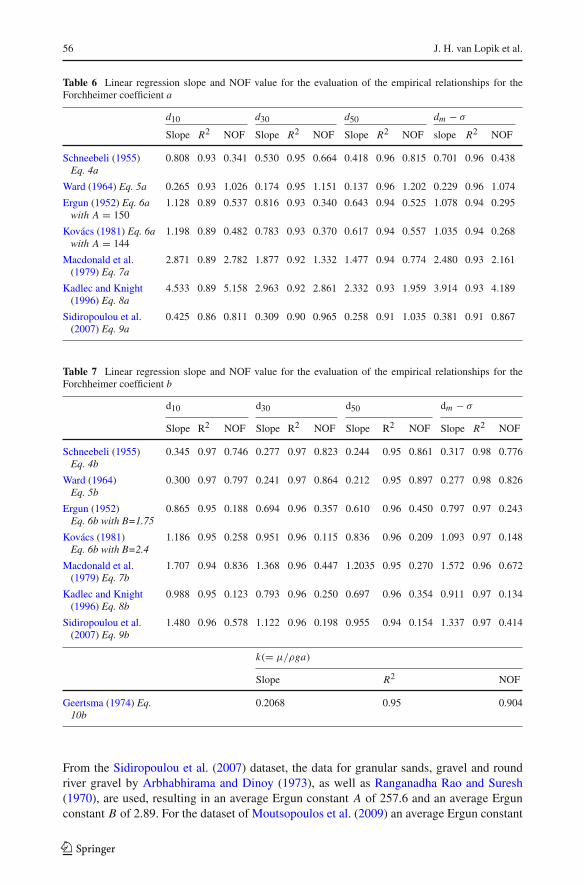
The NOF criterion and the linear regression method (mentioned in Sect. 3.4) are used toevaluate the reliability of the empirical relationships provided in Table 1. The entire datasetof both reference and composite sands is used for the analysis. Considering the median grainsize (d50), the relationships of Ergun (1952), Macdonald et al. (1979) and Kovács (1981)seem to provide the most accurate estimation for coefficient a with regression slopes of 1.48,0.64 and 0.62, respectively (Table 6). For coefficient b, Macdonald et al. (1979) and Kovács(1981) obtained the best fits, resulting in a regression slope of 1.20 and 0.84, respectively(see Table 7). The accuracy of Macdonald et al. (1979) and Kovács (1981) is also confirmedby the NOF analysis (see Tables 6, 7). Overall, the relationship of Macdonald et al. (1979)overestimates the flow resistance, while Ergun (1952) and Kovács (1981) underestimate the

123


Fig. 6 a Forchheimer i − q plot for different mixtures of quarry carbonate rocks and b the associated grainsize distributions (obtained fromMoutsopoulos et al. 2009). Increased d30 results in decreased flow resistance(lower a and b coefficients) compared to the reference material M3

flow resistance, using the median grain size (d50). The relationship by Sidiropoulou et al.(2007) seems to be reliable for the estimation of the coefficient b using d50, while a poorfit was obtained for coefficient a. In order to investigate the empirical relation of Geertsma(1974), the intrinsic permeability was calculated from the determined a coefficient from ourexperimental dataset. A poor estimation of the coefficient b was obtained.

Generally, the use of the characteristic pore length dm − σ in the empirical relationships(Eqs. 4a–9a) results in the best estimates for coefficient a, except for Macdonald et al.(1979) and Kadlec and Knight (1996). Macdonald et al. (1979) also results in poor estimatedfor coefficient b. For both Ergun (1952) and Kovács (1981), the best estimations for bothcoefficienta and coefficientb are obtained.Also, the use ofd10 results in reasonable regressionslope values. However, for the estimation of coefficient a while using d10, the data are morescattered around the regression line, resulting in a R2-coefficient of 0.89, while 0.94 isobtained for dm − σ .

4.4.1 Derivation of Ergun Constants Based on the Experimental Dataset

The Ergun constants A and B are determined for our dataset following the linear regressionprocedure (mentioned in Sect. 3.4). This is done for the median grain size (d50), as well asfor d10, d30 and dm−σ . Using the median grain size (d50), or d30, the Ergun constants basedon our experimental dataset are higher than the values provided by Ergun (1952) and Kovács(1981) (Table 8).

In the literature, a wide range of different values of the Ergun constants can be found.According to Du Plessis (1994) analytical study on flow behavior in the nonlinear laminarflow regime, higher constants A and B in the range of 200 and 1.97 should be used. TheErgun constant B of 2.88 (d50) and 2.53 (d30) is in agreement with the value provided byEngelund (1953), who stated that a value of approximately 2.8 should be used for uniformand rounded sand grains. The range of typical suitable experimental Ergun constants forsands and gravel in the literature is large. The dataset of sand and gravel in Macdonald et al.(1979) provides an average Ergun constant A of 254.4 (range of 142–488) and an averageErgun constant of 2.024 (ranging from 2.52 to 1.01). Analysis of the Li et al. (2017) datasetresults in an average Ergun constant A of 349.6 and an average Ergun constant B of 1.786.

123


Table 6 Linear regression slope and NOF value for the evaluation of the empirical relationships for theForchheimer coefficient a

d10 d30 d50 dm − σ

Slope R2 NOF Slope R2 NOF Slope R2 NOF slope R2 NOF

Schneebeli (1955)Eq. 4a

0.808 0.93 0.341 0.530 0.95 0.664 0.418 0.96 0.815 0.701 0.96 0.438

Ward (1964) Eq. 5a 0.265 0.93 1.026 0.174 0.95 1.151 0.137 0.96 1.202 0.229 0.96 1.074

Ergun (1952) Eq. 6awith A = 150

1.128 0.89 0.537 0.816 0.93 0.340 0.643 0.94 0.525 1.078 0.94 0.295

Kovács (1981) Eq. 6awith A = 144

1.198 0.89 0.482 0.783 0.93 0.370 0.617 0.94 0.557 1.035 0.94 0.268

Macdonald et al.(1979) Eq. 7a

2.871 0.89 2.782 1.877 0.92 1.332 1.477 0.94 0.774 2.480 0.93 2.161

Kadlec and Knight(1996) Eq. 8a

4.533 0.89 5.158 2.963 0.92 2.861 2.332 0.93 1.959 3.914 0.93 4.189

Sidiropoulou et al.(2007) Eq. 9a

0.425 0.86 0.811 0.309 0.90 0.965 0.258 0.91 1.035 0.381 0.91 0.867

Table 7 Linear regression slope and NOF value for the evaluation of the empirical relationships for theForchheimer coefficient b

d10 d30 d50 dm − σ

Slope R2 NOF Slope R2 NOF Slope R2 NOF Slope R2 NOF

Schneebeli (1955)Eq. 4b

0.345 0.97 0.746 0.277 0.97 0.823 0.244 0.95 0.861 0.317 0.98 0.776

Ward (1964)Eq. 5b

0.300 0.97 0.797 0.241 0.97 0.864 0.212 0.95 0.897 0.277 0.98 0.826

Ergun (1952)Eq. 6b with B=1.75

0.865 0.95 0.188 0.694 0.96 0.357 0.610 0.96 0.450 0.797 0.97 0.243

Kovács (1981)Eq. 6b with B=2.4

1.186 0.95 0.258 0.951 0.96 0.115 0.836 0.96 0.209 1.093 0.97 0.148

Macdonald et al.(1979) Eq. 7b

1.707 0.94 0.836 1.368 0.96 0.447 1.2035 0.95 0.270 1.572 0.96 0.672

Kadlec and Knight(1996) Eq. 8b

0.988 0.95 0.123 0.793 0.96 0.250 0.697 0.96 0.354 0.911 0.97 0.134

Sidiropoulou et al.(2007) Eq. 9b

1.480 0.96 0.578 1.122 0.96 0.198 0.955 0.94 0.154 1.337 0.97 0.414

k(= μ/ρga)

Slope R2 NOF

Geertsma (1974) Eq.10b

0.2068 0.95 0.904

From the Sidiropoulou et al. (2007) dataset, the data for granular sands, gravel and roundriver gravel by Arbhabhirama and Dinoy (1973), as well as Ranganadha Rao and Suresh(1970), are used, resulting in an average Ergun constant A of 257.6 and an average Ergunconstant B of 2.89. For the dataset of Moutsopoulos et al. (2009) an average Ergun constant

123


Table 8 Estimation of the Ergunconstant A and B with linearregression analysis at γ = 1.00using all sand samples

Particle size Ergun constant (Eq. 7) Slope R2 NOF

d50 A 233.5 1.00 0.94 0.260

B 2.88 1.00 0.96 0.113

d10 A 120.3 1.00 0.89 0.330

B 2.03 1.00 0.94 0.124

d30 A 183.8 1.00 0.93 0.275

B 2.53 1.00 0.96 0.106

dm − σ A 139.1 1.00 0.94 0.254

B 2.20 1.00 0.97 0.095

A of 220.4 (range of 144.7–429.2) is derived using d50, while the derived Ergun constant Afor cobbles is erroneously high (value of 1963). The average Ergun constant B is 2.26 (rangeof 1.95–3.39). The Ergun constants provided by these studies on nonlinear flow behavior ingranular material compare well to the values we have obtained in this study.

The use of a smaller grain size d30, as well as dm − σ , for the characteristic pore length,and their associated derived Ergun constants, obtained approximately similar NOF valuesand R2-coefficients for the regression line (see Table 8) as compared to fitting analysis usingd50. The fits using d10 are less accurate.

4.4.2 Ergun Constants and the Effect of Finer Material

In order to investigate the effect of the different grain size distributions of the composite sandswith respect to the reference sands, linear regression analysis is applied to the reference sandsS.3–8 and the corresponding sandmixtures (see Fig. 7; Table 9). The Ergun constants derivedfrom the entire dataset of this study were used (see Table 8). The use of d30 and dm − σ andassociated Ergun constants A and B results in only a slightly better fit with the experimentalForchheimer coefficients. It should be noted that small variations in porosity between thereference and composite sands (see Tables 2, 3) affect the prediction of coefficient a andcoefficient b using equation 6. Note that the d30 for the composite sands is decreased byfactors ranging between 0.81 up to only 0.96. Hence, the characteristic pore length of d30might provide better estimations for the Forchheimer coefficients for well-graded sands witha significant increase in finer material (significantly decreased d30 values) with respect touniformly graded sands at approximately equal porosity values. The same holds for theuse of dm − σ . However, compaction of typical well-graded sandy soils with wide grain sizedistributions normally results in reduced porosity values compared to uniformly graded sands.

4.5 Friction Factor

The friction factor calculated with Eq. (12) is plotted versus the Reynolds number Res inFig. 8. We used regression analysis on our full dataset to obtain the following relationship:

f = 1340

Res+ 19.35; R > 0.96 (21)

At Reynolds numbers Res higher than 9000, f < 19.5. This means that in this case Forch-heimer equation reduces to bq2 and flow can be considered fully turbulent (Andersen andBurcharth 1995; Venkataraman and Rao 1998; Salahi et al. 2015). Our results are in agree-

123


Fig. 7 a Analysis of the reference sands (S.3–8) and all composite sands using the relationship of Ergun(1952) (see Eq. 6) for Forchheimer coefficient a, and b Forchheimer coefficient b

Table 9 Analysis of thereference sands (S.3–8) and allcomposite sands using therelationship of Ergun (1952) withthe Ergun constants provided inTable 8

Particle size Ergun constant (Eq. 6) Slope R2

d50 A 233.5 1.0502 0.89

B 2.88 1.0464 0.93

d10 A 120.3 0.9595 0.96

B 2.03 1.02 0.86

d30 A 183.8 1.0021 0.97

B 2.53 1.032 0.93

dm − σ A 139.1 1.0001 0.95

B 2.20 1.032 0.95The used data are plotted inFigure 7

ment with Salahi et al. (2015), who obtained f = 967Res

+ 9.45 with a R2 of 0.98 for theirexperimental dataset on coarse granular material.

We have also followed the method of Herrera and Felton (1991) to relate the friction factorto their proposed Reynolds number ReH :

f = 822.3

ReH+ 13.16; R2 > 0.95 (22)

Herrera and Felton (1991) proposed their form of the Darcy–Weisbach equation for well-graded coarse material. However, the composite sands in our dataset are only slightly morewell-graded compared to our reference dataset (Cu < 1.8). Hence, no large differencebetween the method of Stephenson (1979) and Herrera and Felton (1991) is found for ourdataset.

123


Fig. 8 The relationship betweenReynolds number ReS andfriction factor f using theStephenson (1979) method

5 Discussion

In this study, nonlinear flow behavior experiments on the composite and the reference sands(S.1–9) were conducted at minimum particle Reynold numbers ranging between 0.26 and16.33 (Tables 4, 5). Hence, it is likely that the majority of the flow dataset at lower Reynoldnumbers is determined at the onset of the nonlinear laminar flow regime. Experimentalstudies on flow behavior in packed uniform spheres determined critical Reynolds numbers(Re > 300) for fully turbulent flow (e.g., Dybbs and Edwards 1984; Seguin et al. 1998).According to Andersen and Burcharth (1995), it is challenging to define the transition fromnonlinear laminar flow to fully turbulent flow for granular, irregular shaped, porous media.Consequently, it is difficult to identify to what extent the fully turbulent flow is developed atincreased particle Reynolds numbers in the coarser material. Overall, the grain sizes of theinvestigated sands in this study are significantly lower than for the sands and gravel in theliterature, and therefore, the observed flow resistance by means of Forchheimer coefficientsa and b is significantly higher (see Fig. 5b).

To date, complete understanding of the macroscopic nonlinear flow behavior at specificReynold numbers for different complex pore structures is hampered due to insufficient knowl-edge about the link between the macroscopic flow characteristics and complex microscopicpore structures. Many attempts have been made to link Forchheimer coefficients a and b, todifferent pore scale parameters. For example, some studies have linked the effect of the tor-tuosity (ratio between effective hydraulic stream line length and straight-line length betweentwo points to characterize fluid pathways) to the Forchheimer coefficient b (e.g., Liu et al.1995; Thauvin and Mohanty 1998). Overall, increased tortuosity of a porous medium resultsin increased flow resistance and, therefore, larger b coefficients. However, it is difficult toobtain the tortuosity for complex pore structures of granular porous media. Moreover, asdescribed in Sect. 2.2, drag forces that determine the nonlinear laminar flow in porous mediaare controlled by the fluid–solid interfaces of the pore structures and pore geometry (e.g.,Hassanizadeh and Gray 1987; Comiti et al. 2000; Panfilov and Fourar 2006). Hence, it seemsreasonable to characterize the porous media by means of the surface area and its roughness.For example, the capillary representation model of Comiti et al. (2000) used a dynamic

123


surface area of the porous media, as well as the tortuosity, while assuming a cylindricalcharacterization of the pores.

The results in Sect. 4.2 show that an increased fraction of finer material at fixed valuesof d50 and porosity results in an increased flow resistance. Under this condition, the use ofthe characteristic pore length by means of the grain size diameter d30 in the modified Ergunrelationships works well for accurate prediction of the Forchheimer coefficients a and b toaccount for finer material.

As mentioned earlier, Macdonald et al. (1979) suggest the use of the Sauter mean (Eq. 11)as a measure of the characteristic pore length in the relationships (Eqs. 6, 7). This definitionof the characteristic pore length emphasizes the importance of specific surface area in com-plex pore structures. Hence, it seems sensible that the nonlinearity in flow resistance due tointerfacial drag forces acting on the fluid–solid interface should be upscaled to a macroscopicparameter that characterizes pore surface area. For grain size distributions considering perfectspherical grains, the d32 can be used. However, formore angularmaterials with lower spheric-ity values, the ratio between volume and surface area is lowered and smaller characteristicpore lengths should be considered. In our study, the d30 of uniformly graded sand approxi-mately equals the Sauter mean, considering rounded sand grains. Herrera and Felton (1991)suggested to use the standard deviation of particle sizes and substituted the characteristicpore length d by dm − σ . For more well-graded sand types, with larger standard deviations,finer particles fill the pores between coarser particles and the contact surface of particles withwater increases. Tables 2 and 3 show that the characteristic pore length of dm − σ is smallerthan d30 and, hence, accounts more for the finer particles in the packed-column sample.

Nonetheless, it should be noted that fitting of nonlinear flow data with the Forchheimerrelation (Eq. 2) over a wide range of Reynold numbers describes the gradual macroscopictransition from laminar Darcy flow to nonlinear laminar flow, and, eventually, to fully tur-bulent flow. Hence, linking between the different macroscopic flow characteristics at a widerange of Reynold numbers and the complex microscopic pore structures by means of , e.g.,characteristic pore length, tortuosity, compaction grade, sphericity is complicated.

6 Conclusions

The current study provides new experimental data on nonlinearwater flowbehavior in variousuniformly graded granular material for 20 samples, ranging from medium sands (d50 > 0.39mm) to gravel (6.34 mm). The effect of the grain size distribution on the macroscopic flowresistance parameters is analyzedusing theForchheimer coefficients.As the reference dataset,we have used 11 uniformly graded filter sands. In addition, the mixtures of the filter sands areused to obtain composite sands with different grain size distributions. This provided sampleswith increased Cu values by a factor of 1.19 up to 2.32 at equal median grain size d50 andporosity relative to the associated reference sands. The main conclusions from this study are:

• Our dataset has shown that the d50 value is not enough to predict flow resistance accu-rately. Wider grain size distributions, indicated by an increase in d10 and d30 for thecomposite sands, result in an increased flow resistance with respect to the referencesands at equal median grain size (d50) The a coefficients increased by factors up to 1.68and the b coefficients increased by factors up to 1.44 with respect to the reference sands.

• The modified Ergun equation could provide accurate estimates of coefficients a and b.The use of Ergun constants A=183.8 and B = 2.53 and the use of d30 as characteristicpore length are suggested to provide good fits. While using the method of Herrera and

123


Felton (1991) with a characteristic pore length of dm − σ , Ergun constants A = 139.1and B = 2.2 are suggested.

• The derived Ergun constants of the current study are in agreement with the Ergun con-stants derived from other experimental datasets.

• Wefound a clear correlation between the experimentally derivedForchheimer coefficientsa and b for our dataset of subangular-subrounded, uniformly graded filter sands at anoptimal compaction grade.

Acknowledgements This work was supported by foundations STW (Foundation for Technical Sciences)and O2DIT (Foundation for Research and Development of Sustainable Infiltration Techniques). The authorsthank Tony Valkering and Theo van Velzen from dewatering company Theo van Velzen for constructing theexperimental setup and Peter de Vet from dewatering company P.J. de Vet & Zonen for optimizing setup. Weare grateful toWillem Jan DirkxMSc for his help and constructive input during the nonlinear flow experimentsFunding was provided by Stichting voor de Technische Wetenschappen (Grant No. 13263).

Open Access This article is distributed under the terms of the Creative Commons Attribution 4.0 Interna-tional License (http://creativecommons.org/licenses/by/4.0/), which permits unrestricted use, distribution, andreproduction in any medium, provided you give appropriate credit to the original author(s) and the source,provide a link to the Creative Commons license, and indicate if changes were made.

Appendix 1

See Fig. 9.

Fig. 9 The grain size distribution characterization (d10, d20, d50 and d60) for the uniformly graded filtersands (S.1–10) and the sand mixtures (S3.1–8.1). Note that the coarse gravel (S.11 with d50 = 6.34 mm) isnot taken into account

123

http://creativecommons.org/licenses/by/4.0/


Appendix 2

See Fig. 10.

Fig. 10 a The i − q plots for the sandy porous media S3.1–8.1 and b the cumulative grain size distributions

123


Fig. 10 continued

References

Ahmed, N., Sunada, D.K.: Nonlinear flow in porous media. J. Hydraul. Div. ASCE 95(6), 1847–1857 (1969)Allen, K.G., von Bäckström, T.W., Kröger, D.G.: Packed bed pressure drop dependence on particle shape, size

distribution, packing arrangement and roughness. Powder Technol. 246, 590–600 (2013)Andersen, O.H., Burcharth, H.F.: On the one-dimensional steady and unsteady porous flow equation. Coast.

Eng. 24, 233–257 (1995)Arbhabhirama, A., Dinoy, A.A.: Friction factor and Reynolds number in porous media flow. J. Hydraul. Div.

ASCE 99(6), 901–911 (1973)Aulisa, E., Ibragimov, A., Valko, P., Walton, J.: Mathematical framework of the well productivity index for fast

Forchheimer (non-Darcy) flows in porous media. Math. Models Methods Appl. Sci. 19(8), 1241–1275(2009)

Bagci, Ö., Dukhan, N., Özdemir, M.: Flow regimes in packed beds of spheres from pre-Darcy to turbulent.Transp. Porous Med. 104(3), 501–520 (2014)

Bear, J.: Dynamics of Fluids in Porous Media. Dover Publications, New York (1972)Blott, S.J., Pye, K.: GRADISTAT: a grain size distribution and statistics package for the analysis for uncon-

solidated sediments. Earth Surf. Process. Landf. 26(11), 1237–1248 (2001)Bordier, C., Zimmer,D.:Drainage equations and non-Darcianmodeling in coarse porousmedia or geosynthetic

materials. J. Hydrol. 228(3–4), 174–187 (2000)Carman, P.C.: Fluid flow through granular beds. Trans. Inst. Chem. Eng. 15, 150–166 (1937)Chaudhary, K., Cardenas, M.B., Den, W., Bennett, P.C.: Pore geometry effects on intrapore viscous to inertial

flows and on effective hydraulic parameters. Water Resour. Res. 49(2), 1149–1162 (2013)

123


Chauveteau, G., Thirriot, C.: Régimes d’écoulement en milieu poreux et limite de la loi de Darcy [Regimesof flow in porous media and the limitations of the Darcy law]. La Houille Blanche 1(22), 1–8 (1967)

Comiti, J., Renaud, M.: A new model for determining mean structure parameters of fixed bed from pressuredrop measurements: application to beds with packed parallelepipepal particles. Chem. Eng. Sci. 44(7),1539–1545 (1989)

Comiti, J., Saribi, N.E.,Montillet, A.: Experimental characterization of flow regimes in various porousmedia—3: limit of Darcy’s or creeping flow regime for Newtonian and purely viscous non-Newtonian fluids.Chem. Eng. Sci. 55(15), 3057–3061 (2000)

Darcy, H.: Les fontaines publiques de la ville de Dijon, p. 647. Victor Dalmont, Paris (1856)Du Plessis, J.P.: Analytical quantification of coefficient in the Ergun equation for fluid friction in packed beds.

Transp. Porous Med. 16(2), 189–207 (1994)Dybbs, A., Edwards, R.V.: A new look at porous media fluid mechanics. Darcy to turbulent. Fundamentals

of Transport Phenomena in Porous Media. Part of the NATO ASI Series book series (NSSE), MartinusNijhoff, Dordrecht, vol. 82, pp. 199–256 (1984)

Ergun, S.: Fluid flow through packed columns. Chem. Eng. Prog. 48(2), 89–95 (1952)Engelund, F.A.: On the laminar and turbulent flows of groundwater through homogenous sand. Danish

Academy of Technical Science, Copenhagen (1953)Fand, R.M., Kim,B.Y.K., Lam,A.C.C., Phan, R.T.: Resistance to the flowof fluids through simple and complex

porous media whose matrices are composed of randomly packed spheres. J. Fluids Eng. 109(3), 268–273(1987)

Fand, R.M., Thinakaran, R.: The influence of the wall on flow through pipes packed with spheres. J. FluidsEng. 122(1), 84–88 (1990)

Firdaouss, M., Guermond, J.L., Le Quéré, P.: Nonlinear correction to Darcy’s law at low Reynolds numbers.J. Fluid Mech. 343, 331–350 (1997)

Forchheimer, P.H.: Wasserbewegung durch boden. Z. Ver. Deutsch. Ing. 50, 1781–1788 (1901)Fourar, M., Radilla, G., Lenormand, R., Moyne, C.: On the non-linear behavior of a laminar single-phase flow

through two and three-dimensional porous media. Adv. Water Resour. 27(6), 669–677 (2004)Geertsma, J.: Estimating the coefficient of inertial resistance in fluid flow through porous media. Soc. Petrol.

Eng. J. 14(5), 445–450 (1974)Hassanizadeh, S.M., Gray, W.G.: High velocity flow in porous media. Transp. Porous Med. 2(6), 521–531

(1987)Herrera, N.H., Felton, G.K.: Hydraulics of flow through a rockfill dam yusing sediment-free water. Trans.

ASABE 34(3), 871–875 (1991)Hill, R.J., Koch, D.L.: The transition from steady to weakly turbulent flow in a close-packed ordered array of

spheres. J. Fluid Mech. 465, 59–97 (2002)Holditz, S.A., Morse, R.A.: The effects of non-Darcy flow on the behavior of hydraulically fractured gas wells.

J. Pet. Technol. 28(10), 1179–1196 (1976)Houben, G.J.: Review: Hydraulics of water wells flow laws and influence of geometry. Hydrogeol. J. 23(8),

1633–1657 (2015)Huang, K., Wan, J.W., Chen, C.X., He, L.Q., Mei, W.B., Zhang, M.Y.: Experimental investigation on water

flow in cubic arrays of spheres. J. Hydrol. 492, 61–68 (2013)Izbash, S.V.: O filtracii V Kropnozernstom Materiale. USSR, Leningrad (1931). (in Russian)Irmay, S.: On the theoretical derivation of Darcy and Forchheimer formulas. Trans. Am. Geophys. Union

39(4), 702–707 (1958)Jafari, A., Zamankhan, P., Mousavi, S.M., Pietarinen, K.: Modeling and CFD simulation of flow behavior and

dispersivity through randomly packed bed reactors. Chem. Eng. J. 144(3), 476–482 (2008)Jolls, K.R., Hanratty, T.J.: Transition to turbulence for flow through a dumped bed of spheres. Chem. Eng. Sci.

21(12), 1185–1190 (1966)Kadlec, H.R., Knight, L.R.: Treatment Wetlands. Lewis Publishers, Boca Raton (1996)Kovács, G.: Seepage Hydraulics. Elsevier Scientific Publishing Company, Amsterdam (1981)Koekemoer, A., Luckos, A.: Effect of material type and particle size distribution on pressure drop in packed

beds of large particles: Extending the Ergun equation. Fuel 158, 232–238 (2015)Lage, J.L.: The fundamental theory of flow through permeable media from Darcy to turbulence. In: Ingham,

D.B., Pop, I. (eds.) Transport Phenomena in Porous Media, pp. 1–30. Pergamon, New York (1998)Latifi, M.A., Midoux, N., Storck, A., Gence, J-N.: The use of micro-electrodes in the study of flow regimes in

a packed bed reactor with single phase liquid flow. Chem. Eng. Sci. 44(11), 2501–2508 (1989)Li, L., Ma, W.: Experimental study on the effective particle diameter of a packed bed with non-spherical

particles. Transp. Porous Med. 89(1), 35–48 (2011)Li, Z., Wan, J., Huang, K., Chan, W., He, Y.: Effects of particle diameter on flow characteristics in sand

columns. Int. J. Heat Mass Transf. 104, 533–536 (2017)

123


Liu, X., Civan, F., Evans, R.D.: Correlation of the non-Darcy flow coefficient. J. Can. Pet. Technol. 34(10),50–54 (1995)

Macdonald, I.F., El-Sayed, M.S., Mow, K., Dullien, F.A.L.: Flow through porous media-the Ergun equationrevisited. Ind. Eng. Chem. Fundam. 18(3), 199–208 (1979)

Mathias, S.A., Todman, L.C.: Step-drawdown tests and the Forchheimer equation. Water Resour. Res. 46(7),W07514 (2010)

Mathias, S.A., Moutsopoulos, K.N.: Approximate solutions for Forchheimer flow during water injection andwater production in an unconfined aquifer. J. Hydrol. 538, 13–21 (2016)

Ma, H., Ruth, D.W.: The microscopic analysis of high Forchheimer number flow in porous media. Transp.Porous Med. 13(2), 139–160 (1993)

Mijic, A., Mathias, S.A., LaForce, T.C.: Multiple well systems with non-Darcy flow. Groundwater 51(4),588–596 (2013)

Moutsopoulos, K.N., Tsihrintzis, V.A.: Approximate analytical solutions of the Forchheimer equation. J.Hydrol. 309, 93–103 (2005)

Moutsopoulos,K.N.:One-dimensional unsteady inertial flow in phreatic yaquifers, induced by a sudden changeof the boundary head. Transp. Porous yMedia 70, 97–125 (2007)

Moutsopoulos, K.N., Papaspyros, I.N.E., Tsihrintzis, V.A.: Experimental investigation of inertial flow pro-cesses in porous media. J. Hydrol. 374(3–4), 242–254 (2009)

Nield, D.A.: Resolution of a paradox involving viscous dissipation and nonlinear drag in a porous medium.Transp. Porous Med. 41(3), 349–357 (2002)

Panfilov, M., Oltean, C., Panfilova, I., Buès, M.: Singular nature of nonlinear macroscale effects in high-rateflow through porous media. C. R. Mec. 331(1), 41–48 (2003)

Panfilov, M., Fourar, M.: Physical splitting of nonlinear effects in high-velocity stable flow through porousmedia. Adv. Water Resour. 29(1), 30–41 (2006)

Ranganadha Rao, R.P., Suresh, C.: Discussion of ‘Non-linear flow in porous media’, by N Ahmed and DKSunada. J. Hydraul. Div. ASCE 96(8), 1732–1734 (1970)

Rietdijk, J., Schenkeveld F., Schaminée, P.E.L., Bezuijen A.: The drizzle method for sand sample preparation.In: Proceedings of the 6th International Conference on Physical Modelling, editor, Laue, Springman,Seward, pp. 267–272 (2010)

Rode, S., Midoux, N., Latifi, M.A., Storck, A., Saatdjian, E.: Hydrodynamics of liquid flows in packed beds:an experimental study using electrochemical shear rate sensors. Chem. Eng. Sci. 49(6), 889–900 (1994)

Salahi, M-B., Sedghi-Asl, M., Parvizi, M.: Nonlinear flow through a packed-column test. J. Hydrol. Eng. 20(9)(2015). doi:10.1061/(ASCE)HE.1943-5584.0001166

Schneebeli, G.: Expériences sur la limite de validité de la loi de Darcy et l’apparition de la turbulence dans unécoulement de filtration. La Houille Blanche 141, 141–149 (1955). (in French)

Scheidegger, A.E.: The Physics of Flow Through Porous Media, 3rd edn. University of Toronto Press, Toronto(1974)

Sedghi-Asl, M., Rahimi, H.: Adoption of Manning’s equation to 1D non-yDarcy flow problems. J. Hydraul.Res. 49(6), 814–817 (2011)

Sedghi-Asl,M., Rahimi, H., Salehi, R.: Non-Darcy flow of water through a packed column test. Transp. PorousMed. 101(2), 215–227 (2014)

Seguin, D., Montillet, A., Comiti, J., Huet, F.: Experimental characterization of flow regimes in various porousmedia—2: Transition to turbulent regime. Chem. Eng. Sci. 53(22), 3897–3909 (1998)

Sen, Z.: Nonlinear flow towards wells. J. Hydraul. Eng. 15(2), 193–207 (1989)Sidiropoulou, M.G., Moutsopoulos, K.N., Tsihrintzis, V.A.: Determination of Forchheimer equation coeffi-

cients a and b. Hydrol. Proc. 21(4), 534–554 (2007)Skjetne, E., Auriault, J.L.: High velocity laminar and turbulent flow in porous media. Transp. Porous Med.

36(2), 131–147 (1999)Stephenson, D.: Rockfill in hydraulic engineering. Elsevier, Amsterdam (1979)Thauvin, F., Mohanty, K.K.: Network modeling of non-Darcy flow through porous media. Transp. Porous

Med. 31(1), 19–37 (1998)Tyagi, A.K., Todd, D.K.: Discussion of ‘Non-linear flow in porous media’, by N Ahmed and DK Sunada. J.

Hydraul. Div. ASCE 96(8), 1734–1738 (1970)Venkataraman, P., Rao, P.R.M.: Darcian, transitional, and turbulent flow through porous media. J. Hydraul.

Eng. ASCE 124(8), 840–846 (1998)Ward, J.C.: Turbulent flow in porous media. J. Hydraul. Div. ASCE 90(5), 1–12 (1964)Wen, Z., Huang, G., Zhan, H.: Non-Darcian flow to a well in a leaky aquifer using the Forchheimer equation.

Hydrogeol. J. 19(3), 563–572 (2011)Wen, Z., Liu, K., Chen,X.: Approximate analytical solution for non-Darcian flow toward a partially penetrating

well in a confining aquifer. J. Hydrol. 498, 124–131 (2013)

123

http://dx.doi.org/10.1061/(ASCE)HE.1943-5584.0001166


Whitaker, S.: The Forchheimer equation: a theoretical development. Transp. PorousMed. 25(1), 27–61 (1996)Yeh, H.D., Chang, Y.C.: Recent advances inmodeling of well hydraulics. Adv.Water Resour. 51, 27–51 (2013)Zhengwen, Z., Grigg, R.: A criterion for non-Dacry flow in porous media. Transp. Porous Med. 63(1), 57–69

(2006)

123

Documents

The Effect of Grain Size Distribution on Nonlinear Flow ... · Transp Porous Med (2017) 120:37–66 DOI 10.1007/s11242-017-0903-3 The Effect of Grain Size Distribution on Nonlinear