POLICY RESEARCH WORKING PAPER 2376

The Effect of Early Economic incentives have apowerful effect on the work

Childhood Development behavior of women with

Programs on Women's Labor children in Kenya. In additiontc increasing the future

Force Participation and productivity of children,government subsidies of

Older Children's Schooling low-cost early childhood

* K n development programs

would increase the number

of mothers who work, thus

Michael M. Lokshin increasing the incomes of

Elena Glinskaya poor households and lifting

Marito Garcia some families out of poverty.They would also increase

older girls' enrollment in

school, by releasing them

from child care

The World Bank responsibilities.

Development Research GroupPoverty and Human Resources

and

South Asia Region

Poverty Reduction and Economic Management Sector Unit

and

Africa Technical FamiliesHuman Development I1

June 2000H

Pub

lic D

iscl

osur

e A

utho

rized

Pub

lic D

iscl

osur

e A

utho

rized

Pub

lic D

iscl

osur

e A

utho

rized

Pub

lic D

iscl

osur

e A

utho

rized

Pub

lic D

iscl

osur

e A

utho

rized

Pub

lic D

iscl

osur

e A

utho

rized

Pub

lic D

iscl

osur

e A

utho

rized

Pub

lic D

iscl

osur

e A

utho

rized

POLICY RESEARCH WOR(KING PAPER 2376

Summary findings

About 20,000 early childhood development centers A high cost for child care discourages householdsprovided day care for and prepared for primary school from using formal child care facilities and has a negativemore than 1 million children aged three to seven effect on mothers' participation in market work.(roughly 20 percent of children in that age group) in * The cost of child care and the level of mothers'Kenya in 1995. The number of child care facilities wages affect older children's school enrollment, but thesereached 23,690 by the end of 1999. factors affect boys' and girls' schooling differently. An

Lokshin, Glinskaya, and Garcia analyze the effect of increase in mothers' wages increases boys' enrollment butchild care costs on households' behavior in Kenya. For depresses girls' enrollment.households with children aged three to seven, they * Higher child care costs have no significant effect onmodel household demand for mothers' participation in boys' schooling but significantly decrease the number ofpaid work, the participation in paid work of other girls in school.household members, household demand for schooling,and household demand for child care. They find that:

This paper - a joint product of Poverty and Human Resources, Development Research Group; Poverty Reduction andEconomic Management Sector Unit, South Asia Region; and Human Development 1, Africa Technical Families - is partof a larger effort in the Bank to study the role of gender in the context of the household, institutions, and society. Copiesof the paper are available free from the World Bank, 1818 H Street NW, Washington, DC 20433. Please contact PatriciaSader, room MC3-632, telephone 202-473-3902, fax 202-522-1153, email address psader@worldbank.org. PolicyResearch Working Papers are also posted on the Web at www.worldbank.org/research/workingpapers. The authors maybe contacted at mlokshinCaworldbank.org, eglinskaya@aworldbank.org, or mgarcial@worldbank.org. June 2000. (35pages)

The Policy Research Working Paper Series disseminates the findings of work in progress to encourage the exchange of ideas about

development issues. An objective of the series is to get the findings out quickly, even if the presentations are less than fully polished. Thepapers carry the names of the authors and should be cited accordingly. The findings, interpretations, and conclusions expressed in this

paper are entirely those of the authors. They do not necessarily represent the view of the World Bank, its Executive Directors, or thecountries they represent.

Produced by the Policy Research Dissemination Center

THE EFFECT OF EARLY CHILDHOOD DEVELOPMENTPROGRAMS ON WOMEN'S LABOR FORCE PARTICIPATION

AND OLDER CHILDREN'S SCHOOLINGIN KENYA

Michael M. Lokshin,1 Elena Glinskaya, and Marito GarciaThe World Bank

Keywords: Kenya, Early childhood development, Labor supply, Schooling decision, Maximumlikelihood, Non-parametric estimation.

Address for correspondence: Michael Lokshin, Development Research Group, World Bank, 1818H Street NW, Washington, D.C., 20433, USA. The findings, interpretations, and conclusions of this paperare those of the authors and should not be attributed to the World Bank, its Executive Directors, or thecountries they represent. We thank Uwe Deichmann for his help and recommendations with GPS dataanalysis, and Andrew Dabalen and Benedicte de la Briere for many stimulating discussions. Xun Wuprovided excellent support in data management.

1. Introduction

About 20,000 early child development (ECD) centers provided day care and prepared for primary

school over 1 million children three to seven years old (about 20 percent of the children in this age

group) in Kenya in 1995, and the number of child care facilities reached 23,690 by the end of 1999.

The number of ECD centers increased 500-fold between 1963 and 1995 as a response to a

rising involvement of women in the labor market and an increase in the number of single-parent

households. Analysis of the 1995 Kenya Welfare Monitoring Survey shows that 30 percent of rural

households in Kenya are headed by women, and over half of all prime-aged (15-45 years old) married

women work in salaried occupations. The popularity of ECD centers also stems from the belief that

participation in ECD programs improves children's chances in primary school entrance exams and

leads to lower dropout rates (Kipkorir and Njenga 1993; Myers 1992).

The government's annual expenditures on ECD programs can exceed its expenditures for one

year of primary education, according to various estimates in developing countries (Wilson 1995).

Such expensive investments in small children compete for resources with many other programs and

projects, and it is important to provide policymakers with information that allows them to judge which

interventions are most beneficial (Gaag and Tan 1999).

The effectiveness of investments in ECD programs is often estimated based on improvements

in the future productivity ofECD graduates. Growing evidence from diverse cultures shows that most

ECD programs of relatively good quality have meaningful short-term effects on cognitive ability, early

school achievement, and social adjustment (Reynolds et al. 1997).2 These direct improvements in

child outcomes are the benefits that policymakers usually consider when making decisions about

public investments in ECD. At the same time, the availability of affordable ECD facilities may offer

indirect benefits (Myers 1996). Among these are increased participation of mothers in market work

and increased school participation of older siblings (usually young girls) who are freed from the child

care chores. The impact of these benefits on the welfare of households with small children can be

2 There is also increasing evidence that interventions can produce medium- to longer-run effects onschool achievement, special education placement, grade retention, disruptive behavior and delinquency, andhigh school graduation (Reynolds et al. 1997).

substantial. Freeing mothers for market work may improve household income status, and since

households with young children and female-headed households tend to be poorer, increased in

availability of ECD services is expected to help alleviate poverty.

Research in the developing countries indicates that other than the mother females in the

household, especially young daughters, act as providers of free child care, releasing mothers for

market work (Pitt and Rosenzweig 1990; Wong and Levine 1992; Tiefanthaler 1997 ; Connelly, De

Graph, and Levinson 1996; Deutsch 1998). Skoufias (1994) studied intrahousehold time allocation

in India and established that time spent in school by girls and boys is negatively correlated with the

mother's wage rate, suggesting that mothers' time and older children's time at home are substitutes.

Deolalikar (1998) examined determinants of primary and secondary enrollment among Kenyan

households and found a high income elasticity of secondary school enrollment. He also found

significant differences in girls' (but not boys') primary and secondary enrollment by the presence of

children under three in the households. The author reports a particularly strong effect for girls of

secondary school age. Conditional on the other determinants of enrollment, the probability that a girl

aged 14-17 is enrolled in secondary school is reduced by 41 percent if there is a child under three

years of age in the household. The corresponding effect for boys is only 5 percent. These results

suggest that when the market child care services are unavailable, owing to high cost or a lack of

facilities, older siblings of young children are more likely to provide child care.

To date only a few studies - for example, Connelly, De Graph, and Levinson (1996), Wong

and Levine (1992), Lokshin (1999) - have researched the relationship between child care and

women's labor market activity in developing or transitional countries. Nearly all of these found that

the price of child care has nontrivial effects on women's work patterns. The results of this paper

fiurther contribute to the understanding of the interdependency of households' decisions about labor

supplies of its members, child care arrangements and schooling, and suggest policies that lead, in

words of Summers (1992), to investing in all the people. Summers emphasizes that the money spent

in developing countries to educate girls is far more productive than any other social sector outlays.

This paper develops a simple theoretical framework of household utility maximization that

yields empirically testable implications for the relationship between the price of child care and

household behavior. We test these hypotheses byjointly estimating a system of reduced-form equations

of the demand for quality of child care, schooling for older boys and girls, and leisure of the mother

2

and other household members using the method of Semi-Parametric Full Information Maximum

Likelihood. This method takes into account the error term correlations between the household demand

equations.

The estimations reveal that mothers' decisions about participating in the labor market are

sensitive to changes in both wages and the cost of child care. Higher wages that mothers can earn

outside the home encourage them to enter the labor force, while higher-cost child care suppresses

maternal employment. Households' decisions about young children's participation in ECD programs

are found to be very sensitive to the cost of care. Higher-cost child care discourages households from

using ECD programs. Both maternal wage rates and cost of care effect school enrollment of school-

age children. The influence of these factors on households' decisions about its children's schooling

is determined by a combination of income and substitution effects. An increase in mothers' wages

raises school participation of boys; in this case the income effect dominates the substitution effect.

But the mothers' wage increase depresses the school enrollment of girls; in this case girls substitute

for the mother in home production. Higher prices for child care have no significant effect on boys'

schooling and significantly decrease the number of girls at school.

The paper is organized as follows: Section 2 describes the data, and section 3 presents

descriptive statistics on the main outcomes of interest and their factors of influence and describes the

system of early childhood development centers in Kenya. Sections 4 and 5, respectively, show the

development ofthe theoretical model, give details ofthe empirical model, and discuss the conceptual

issues involved in estimating a consistent model of household child care choice, schooling and labor

supply. Section 6 presents and discusses estimation and simulation results. Section 7 concludes with

a discussion of the policy implications and a summary of the findings.

2. Data

The data for this research come from two sources. The 1994 Kenya Welfare Monitoring Survey (WMS

II) provides information on 10,860 households (59,200 individuals), including about 6,624 households

with children between ages three and seven. The survey is based on the multistage sampling

3

framework drawn by the National Sample Survey and Evaluation Program.3 The survey includes

questions on the modes of child care arrangements made for the children in the household, and the

amount of money paid for formal child care. The part of the questionnaire administered to each

individual household member yields data on each household member's labor activity and earnings.

The part of the questionnaire administered to one respondent per household on matters that affected

the household collectively yields information on nonwage household income and on the household's

composition.

Information about child care facilities was collected by the Kenyan Ministry of Education with

the help ofthe World Bank in 1995. A survey was conducted on a sample of more than 800 child care

facilities in 17 districts or urban centers in Kenya, representing urban, pastoralist, and other rural

areas. The Kenya Early Childhood Development Centers Survey (KECDCS) is a stratified random

sample that represents each ofthe sponsorship types in the country. The survey collected information

on the center's location, enrollment, operating expenditures, financial status, and facilities. Data on

the characteristics and salaries of teaching and nonteaching staff, the extent of turnover, and child

feeding practices were collected. For more infornation about the sample selection procedure and

descriptive statistics of the sample, see Mukui and Mwaniki (1995).

There is no direct way to match the data from these two surveys. However, WMS II provides

exact geographical coordinates for most households in the sample, and the addresses of the surveyed

child care facilities were registered in KECDCS. The geographic coordinates of the towns in which

the ECD centers are located were determined using a gazetteer maintained by the U.S. National

Imagery and Mapping Agency.4 The same source was used to identify the location of some of the

households for which no location information was available in the survey. We identified the

administrative district in which each household and ECD center is located by using a so-called point-

in-polygon operation in a geographic information system.5

3WMS II was designed to cover the remote and low-density northen districts but was not fullysuccessful in getting information in those areas.

4 The information is available at http://164.214.2.59/gns/html/index.html

5 The digital map of Kenyan districts that we used was produced by the International LivestockResearch Institute in Nairobi, Kenya.

4

3. Descriptive analysis

Household child care choice and members' labor supply in Kenya

A household's decision about the labor supply of its members is determined to some degree by

comparing members' productivity at home and in the labor market. Small children require constant

care, and a mother's productivity at home is in many cases higher than her potential return from outside

work. Table 1 shows the proportion of mothers working in cash occupations (henceforth working

mothers or employed mothers) by the number of children zero to six years old and by age of the

mother. For all age groups the percentage of working mothers declines with the number of small

children in the household. The employment rate of young mothers (age 18 to 25) is lower than the

employmentrate of the mothers from older age groups. Most economically active are 26- to 35-year-

old mothers. Among them the rate of employment reaches 46 percent for women with one child, which

is comparable to or higher than the proportion of working women with no children. In households with

four or more children below age six, only about 25 percent of mothers work for a wage.

Table 2 presents data on the percentage of working mothers by the household size and by

mother's age group. The higher the size of the household, the lower the probability that the mother

works. Again, as in Table 1, the most active group of mothers is the women 26-3 5 years of age from

small families. These are probably single mothers with small children. For single-mother households

the proportion of working mothers is consistently high, with more than 80 percent ofthe women with

children age 26-3 5 participating in the labor market. Without other adult household members, such

households may depend more heavily on market-provided care. Older mothers with small children

tend to work less.

Adult household members other than the mother, especially nonworking members, may

participate in household production and substitute for the mother as child care providers when she

works. Table 3 shows the probability of households' sending their children to ECD centers by the

number of elderly in the household. The data indicate that the more members of older age are present

in the household, the less likely it is for the child to attend a center.

The labor force participation rates of women with children are lower than they are for other

population groups. Table 4 shows the levels of employment for the various age-gender categories.

5

Rates of employment of men in all age categories in Kenya are significantly higher that the rates of

employment for women. About 70 percent of men in 26-35 year old category work, compared with

only 33 percent of women with children in the same age category. The level of labor force

participation is declining for older age groups, and for the respondents older than 45 years old twice

as many men as women work outside home.

The ECD system in Kenya

Kenya has a long tradition of preschool education. The first privately run preschools appeared in the

1 940s, catering exclusively to the European and Asian communities. Later, day care centers became

established on coffee, tea, and sugar plantation and in urban centers. The expansion of preschools

happened after independence in 1963.

In the mid-1990s the majority of ECD centers in Kenya functioned as community-operated

programs. The other types of early education and care centers were established and run by religious

organizations, private individuals and companies, plantations, estates, NGOs, and local authorities.

Altogether, they represent about 40 percent of all centers in the country.

An organized curriculum for Kenya ECD centers was not established until the late 1980s. By

the mid-1990s, the central government assumed responsibility for training preschool teachers,

supervising and inspecting preschool programs, and developing a locality-specific curriculum. All

but the local government-run centers rely heavily on fees for paying their day-to-day operating

expenses. The majority of ECD funds are spent on teacher salaries.

The prices charged by ECD programs vary considerably. Fees are not set nationally, but rather

by village or urban dwelling parent-teacher associations. Fees vary depending on the quality of

preschools. Centers that employ more educated teachers, have smaller classes, and provide food and

other enhancing activities charge higher fees (Glinskaya and Garcia 1999). Land, buildings, furniture,

and teaching and playing materials are donated by churches, local authorities, and parents themselves.

6

4. Theoretical model

The analysis applies to households with young children. We assume that there are four forms of child

care available to households in Kenya: child care provided by the mother, child care provided by

other adult household members, child care provided by older siblings, and formal (paid) child care.

For households with children and two parents, the husband is considered a potential provider of free

child care. In a household with a single mother who has no relatives living with her, it is assumed that

any informal child care is provided by children themselves or relatives who live outside the

household.

The theoretical model used in this paper is based on the assumption that household members

make choices about their consumption of child care quality, quality of children's schooling, market

goods, and leisure. A household's decisions about the quality of child care and education for its

children and about the amount of time each member of the household can work are motivated by the

desire to achieve the highest level of household welfare.

The model is made tractable through a number of simnplifying assumptions. First, it is assumed

that children require continuous care. Second, the household structure and the number of children are

assumed to be exogenous6 . Third, it is assumed that household members derive utility from the quality

of child care they choose. This utility is represented by the discounted value of a potential

improvement in children resulting from a higher quality of child care or by the current utility of the

family knowing that their children are in competent hands. Fourth, it is assumed that household

members derive utility from the education of children of school age. This utility may be thought of as

benefits that parents receive from well-educated children in the form of, for example, support in old

age and the satisfaction of having educated children. Fifth, we assume that the total time available to

children of school age can be divided into time spent caring for younger siblings and time spent on

schooling. Sixth, it is assumed that mothers spend all their free time on child care - that is, the

mother's leisure time equals the time she spends caring for children.

6 This is a restrictive assumptions, however, work by Blau and Robins (1988) and Conelly, et. al.(1997) suggest that treatin the fertility decision as endogenous does not significantly change the results onhousehold child care modes and household members' labor force participation decisions.

7

In the one-period utility mraximization problem the household chooses its consumption of a

Hicksian composite good G, the quality of child care Q, the quality of education S, the leisure time of

the mother L4, and the leisure time of other household members Lo subject to its budget and time

constraints. The household utility function is assumed to be twice continuously differentiable and

quasi-concave:

MaxU = U(Lm,Lo,G,Q,S)- (11)

The total quality of child care Q is a function of the exogenous quality of the child care provided by

the mother Qm, the exogenous quality of care provided by siblings Qs, the quality of child care

purchased on the market Qp, and the exogenous quality of child care provided by relatives Qo:

Q =Q(Qm,Lm,Qp,Q.o,T Q5,Ts), such that Q'>O and Q"<O (1.2)

where To is the time other household members spend on child care and T, is the time that older siblings

spend on child care.

The education production function is defined to be a continuous, twice continuously

differentiable function S of the time children spend at school:

S = S(1 - T,-), such that S' > 0 and S " < 0 (13)

The budget constraint includes total household expenditures on child care as a function ofthe number

of children in the household, the per-unit quality price of child care, the quality of formal care, and

the time children spend in care:

G = E + WmHm + W,H.-N Pq Qp(Hm-To-T), (1.4)

where E is the exogenous nonwage household income, Hm is mother's time at work, Ho is the other

household members' work time, N is the number of children ages three to seven years old in the

household, Pq is the exogenous price per unit of quality of formal child care, Wm is the market wage

available to the mother, WO is the market wage available to the other household members, and the price

of the composite good G is taken as a numeraire.

Finally, under the assumption that children require constant care, the model specifies the time

constraints affecting the mother, the other household members, and the children:

Lm+H H =L 0 +H,+ T =S+Ts =1 (1.5)

H. - T.-T, > O (1.6)o < T,,, H,, T, S,L L_ H_ < 1 (1.7)

8

The household simultaneously solves its utility maximization problem for an optimal consumption of

all goods that enter into the household utility function.

The structural form household demand equations can be derived from the first-order conditions

(FOC) ofthe household utility maximization problem (1.1-1.7). The structural form demands are the

functions of both endogenous and exogenous variables:

H. = Hm.(Q,Ho,Wm . EW , W, ) HQ= 0'Q(H,S,Ho Wm (1.8)

S=(Hm,QH,rWmsWosEsPq E Ho Ho(Hm,SiQ,Wm,Wo,E,1%s)

Solving the FOC with respect to L,,, Lo, Tw, Ts and Qp, the reduced-form demand system for child care

and schooling, the mother's labor supply, and the labor supply of other household members can be

derived as a function of the exogenous variables. The derived reduced-form demand functions are

then:

H.= Hm(Wm,W.,E,Pq, Q Q= Q(W1% W,E, Pq* (1.9)S = S(Wm,W, EJP,- ) Ho = H(.(W.9W.,E,Pg )

The next section develops an empirical model and discusses specifications for possible estimations

of the household demand systems.

5. Empirical model and specifications

We specify a linear approximation ofthe system of household demand equations (1.8) and (1.9). They

are (substituting H,, Q, S, and Ho on four variables D,'s):

D, = JX + alPq + a21 Wl + a22*o + Ei = ...4, (2.1)

where X is a vector of explanatory variables, p and a's are vectors of pararneters, and e, is an

equation-specific disturbance. Forthe structural demand system (1 .8)Xwould include both exogenous

and endogenous variables, and for the reduced-form demand equation system (1 .9)Xwould include

only exogenous variables. We separate wages and child care price from other explanatory variables

in equation (2.1) because we use predicted values (hat on the top) for these variables obtained from

the different estimations.

The error terms e, of equation (2.1) are likely to be correlated. The demand for each particular

good is an explicit function of other endogenous variables in the system in the case of the structural

form equations, and the error terms are correlated even in the reduced-form demand system equations

9

In the data we do not observe actual household demand. What we do observe are the binary

indicators (demand index functions) that correspond to the latent demand variables and are in the form:

Di=l if D, >OD, = 0 otherwise, i = 1...4 (2.2)

There are several options for estimating the system of equations (2.2). These range from ordinary least

squares to estimating the fully simultaneous system of equations when each equation in the system

includes as explanatory variables the dependent variables from the other three equations. The first two

methods we describe below fall into a category of unconditional demand estimators, as they estimate

demand for every good unconditional on other choices, while the last method estimates a conditional

household demand system.

The simplest estimations of the demand system can be obtained by using binary technique -

for example, a linear probability model or binary probit estimation. However, this method imposes

an assumption of independence of the error terms between the system of equations (2.1). The

coefficients estimated by four independent probits will be unbiased but inefficient in a general case.

It is possible to estimate the household demand system by specifying ajoint distribution ofthe

error terms in (2.1). For example, under an assumption ofjoint normality of the distribution of error

terms, the system of equations (2.1) can be estimated by Full Information Maximum Likelihood

(FIML).

Finally, the structural form of the household demand system can be estimated as a system of

simultaneous equations, a so-called conditional demand system. This approach, however, presents two

major problems. First, it is very hard to find and to justify a choice of identifying variables. Second,

in the case ofthe fully simultaneous system of equations with binary dependent variables, there exists

a problem of logical consistency (see, for example, Maddala 1983, p. 214) that makes it impossible

to estimate this system of equations without imposing restrictive assumptions that may have no

economic interpretation.

Thus, the best estimation method in this situation is the estimation of the reduced-form

household demand system under an assumption that all error terms in equations (2.2) are correlated.7

7This estimation method allows us to account for the unobserved variables, uncorrelated with theexplanatory factors, to influence outcomes. For example, the presence of mothers' siblings in the area ofresidence or the existence of neighbor-help groups, while uncorrelated with the explanatory variables, canhave an effect on all outcomes of interest.

10

For estimation we use the Semi-Parametric Full Information Maximum Likelihood (SPFIML) method

developed by Laird (1978), and Heckman and Singer (1984), and applied to simultaneous equations

by Mroz and Guilkey (1992), and Mroz (1999). The method allows us to estimate the system of

simultaneous binary equations without specifying an exact functional form ofthe joint distribution of

the error terms e, and approximating these distribution non-parametrically. The method should provide

more efficient estimators than FIML in a general case and is far less computationally expensive.

To account for possible error correlations we impose a factor structure on the disturbances

in equations (2.1):

£ii pfj + ' V +P2YiV + p3iV X i = 1...N, j = 1 ... 4 (2.3)

where i is a household index, j is an equation index, N is a total number of observations, [2 is an

independent extreme value error. VI, V2, and V3 are common factors among the equations. These

factors are unobservable variables that influence the choices made by households and that are

uncorrelated with the explanatory variables. pI, P2, and p3, are factor loadings that represent the effect

of a given factor in each equation. We introduce a three-factor structure to account in the most

unrestricted form for the possible sources of heterogeneity in the disturbances.8

We assume that the distributions of the v's in equations (2.2) may be approximated by the

following step functions:

Pr(VI =Vlk) = Pk , Pk 2 0 and E Pk 1 (2.4)k=1

Pr(V2 =V 2 1) = P, PI 2 0 and P =1 (2.5)1=1

M

Pr(V3 = V 3m) = Pm. Pm > 0 and ZPm = 1 (2.6)m=1

where v's are the points of support in the distribution of the factors, P's are the probabilities that the

factors take value v, and K, L, and Mare the numbers of points of support of the distribution of each

factor.

Then the likelihood function describing the mother's labor force participation decision,

younger children's child care mode, older children's school participation, and other household

members' work decisions is given by:

8 For a discussion of the choice of the optimal number of factors, see Anderson and Rubin (1956).

11

NLg K L M 4 >

r = L PRz(xzbzlVk VI, V, (2.5)i=l ksI 1=1 M=I z=1

where the probability terms, denoted by PRz(.), are the cumulative distribution functions for every

demand index function, and N is the total number of observations in the sample.

Choosing a priori numbers of points of support K. L, and MA the log-likelihood function Z§ is

maximized over ,B's, p's, Ps, and v's. For identification purposes, the two points of support for both

factors are normalized to equal 0 and 1, respectively.9 The number of points of support is increased

until the difference in the log-likelihoods of consequent maximizations satisfies the convergence

criteria.10 The variance-covariance matrix e of the estimated coefficients in the model (2.1-2.2) is

estimated by approximating the asymptotic covariance matrix by so-called "sandwich" estimator (see,

for example, Davidson and MacKinnon 1993, 263).

Dependent variables

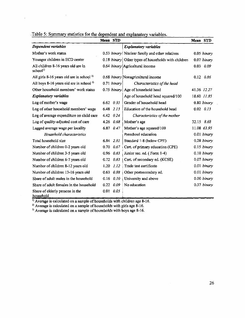
Summary statistics for the dependent variables of the system (2.1) are shown in Table 5. The

definitions of dependent variables are the following:

Mother's workstatus: We define as households with a working mother the households where

a mother is reported to be working for cash and receiving wages. More han half of the households

with small children have working mothers.

Household use ofchildcarefacilities: The households where at least one ofthe children aged

three to six are in ECD centers are classified as the households that use paid child care facilities.

About 18 percent of households use child care facilities as a form of day care for their children.

9 The functional form for the normalization of probability weights, the points of support for thelikelihood function (7), and the estimated parameters are given in the Appendix.

10 We use a likelihood ratio X2-test at a significance level of 25% to determine the rejection oracceptance of the model with one point of support. If the model without heterogeneity is accepted in favorof the model with the control for unobserved heterogeneity, no further search is done. If the simple modelspecification is rejected, than we perform a x2'test for whether to accept or reject the two points of supportspecification versus a three points of support model,etc.

12

Household school participation: The indicator dummy variable is equal to 1 for the

households where all children of a school age were attending school; otherwise this dummy variable

is equal to 0. About a quarter of Kenyan households have at least one school-age child not in school.

Working status of other household members: Households with working "other household

members" are those where at least one adult household member is reported to be working for cash

wages. Seventy-five percent of households are classified as households with working "other

members" according to this definition.

Explanatory variables

The definitions and descriptive statistics for the explanatory variables in the system of equations (2.2)

are presented in Table 5. Several key variables of interest are discussed in detail below.

Price per quality unit of child care (P): We identify the effect of child care prices on

household behavior through district-level differences in these prices. There are two main sources of

information about the child care prices. First, on the household level, information about total

household expenditures on child care for the last month is available from the WMS II. Second, fees

charged by day care facilities were reported in the facility questionnaire collected in KECDCS.

Ideally, we would like to have child care prices from the ECD centers that are in the choice

set of every household. Neither source of prices provides us with such information. The household

expenditure on child care is endogenous to the child care prices and represents the price in only one

child care facility, chosen by the household. The child care facility survey clearly does not cover all

ECD centers in a particular area, and only about 75 percent of the district surveyed by the household

survey is covered by the facility survey. In this research we use both approaches to child care price

estimation and compare the results based on the different measures.

Estimating care prices from the household expenditures on child care, we, following Blau and

Robins (1988), Blau and Hagy (1998) assume that the price per unit of quality of child care is uniform

within a district'" and use the average district-specific household expenditure as a proxy for the child

care price.

The average prices of child care are calculated for 43 districts.

13

To calculate the price of care based on the information on centers' fees, we estimate the

quality-adjusted price of outside-home care using the method suggested by Blau and Hagy (1998).

KECDCS collected extensive information about the characteristics ofthe child care provided and the

fees charged. These data are used to estimate a model of fees for formal child care facilities. The

quality-adjusted price of an hour of child care is determined by a location-specific hedonic price

equation:

p = nk +P Xi + Ei

where Pi is the price of the formal care at the ECD center, x, is a vector of variables that represents

the characteristics of the facility, p is a vector of coefficients, E, is an error term. In that specification

ltk can be interpreted as a market-specific, quality-adjusted, hourly price of ECD program in the

location k.

We use the quality-adjusted price of care to compare the effects of price on household

behavior for facilities that offer different quality of care. For example, suppose one facility offers

several developmental programs and has a low teacher-child ratio. In other words, that facility

provides a high quality of child care but charges a relatively high price for its services. The other

institution does not offer such high quality of care, and the price it charges is low. Directly comparing

the prices of these two facilities is not possible because these prices are charged for different

services. The methodology suggested above allows us to adjust prices for differences in the quality

of provided care and thus makes these quality-adjusted prices comparable.

Mother's offered wage (Wi): The wage rates available to each mother have been imputed

using Mincer's (Mincer and Polachek 1974) type earning function regression with a control for

selectivity. 2 We use the SPFIML approach described above as an alternative to the standard Heckman

correction procedure. This semi-parametric method allows us to relax an assumption of joint

normality of the error term of regression and selection equations. The method is applied to a

subsample of women working in cash occupations. Monthly earnings have been calculated as a ratio

12 Regression coefficients for the wage equations are shown in Appendix 2. For identification in theselection equation we use lagged district-specific unemployment rates, calculated from the 1992 KenyaWelfare Monitoring Survey.

14

of the reported women's earnings and the number of months she worked during the period of time for

which she chose to report her earnings.'3

In the wage regression, the following explanatory variables have been used to predict mothers'

monthly earnings: the mother's educational level, her age, the number of children she had (as a proxy

for work experience), her marital status, and the number of year she spent in her current main job.

Imputations are made based on the women's predicted monthly earnings with the job tenure of

nonworking mothers being equal to zero. Here the offered wage is assumed to be a wage that a mother

could earn if she were to start a new job.

Offered wages of other household members (Wd: The wage rates available to other

household members are calculated similarly to the wage rates available to mothers. Different

regressions were run to predict wages for household members of different ages and genders. After the

imputations, two methods were used to obtain the wage WO. Under the first specification the offered

wage of other household members is equal to the lowest potential wage that can be earned by any

household member except the mother. The second specification uses the average potential wage that

can be earned by adult household members except the mother as an explanatory variable in the model.

Nonwage household income: Nonwage incomes are measured as householdmonthly income

from all sources other than wages. We divide the total household nonwage income into two parts. The

first measure includes income from agricultural sales, and the second one includes income from

business activities, pensions, other transfers, and the other incidental income.

Other explanatory variables include the mother's age and her level of education, household

size and demographic composition, and the number of children from various age groups, as well as

the average level of wages in the district.

6. Results and simulations

The results of the estimation of the system of simultaneous equations (2.2) by SPFIML are presented

for the specification with three points of support for each of the three common factors in the model.

Further increasing the numbers of points of support did not significantly increase the value of the

13If a woman, for example, reported her earnings for week, these were adjusted to a monthly basis.

15

likelihood function. The estimated coefficients are shown for the model estimated with and without

adjusting for unobservable heterogeneity and correlation of the error terms. The estimation of the

model without adjusting for a possible correlation in the error terms between equations (2.2) is

essentially a joint yet independent estimation of four probits.

The equation for the older children's schooling in both SPFIML and independent probits cases

is estimated only for the sample of households that have school-age children. The contribution to the

likelihood function from this equation for the households with no school-age children is set equal to

unity when four equations are estimated simultaneously, and households without school-age children

are excluded from the estimation in the case of independent probits.

Tables 6(a) and 6(b) present the estimated coefficients for the specification ofthe model (2.2)

where we use the average local household expenditure on child care as a proxy for the price of child

care. According to the likelihood-ratio test criterion, the independent specification is rejected in favor

of the SPFIML estimation.14

Both SPFIML and independent probits estimations show that the price of care has a negative

effect on maternal employment. The higher the potential market wage rate of the mother, the more

likely the mother will participate in the labor force. Mothers from single-parent households, younger

mothers, and mothers from households where the education of the head is higher are more likely to

work.

The results of the estimation indicate that a high price of care decreases the probability that

the household will use outside-home care. Households where the mother has a higher market wage rate

are significantly more likely to use paid care. The number of children in a household is negatively

related to the household's likelihood of using ECD centers. Here, one explanation could be the

existence of some economy of scale based on the number of children that increases the productivity

of other household members at home. In other words, once someone is taking care of one child, they

can take care of two, whereas if the household put these children in a child care center it would have

to pay double the price. An important finding is that the presence of older children has a significant

14 The log-likelihood value for the independent estimates is -11672.12 based on 164 parameters.The log-likelihood value for the SPFIML estimate is -11327.38 based on 182 parameters. This is anincrease of 344.74 in the log-likelihood value for 18 additional parameters.

16

negative effect on the paid care use. This fact may support the hypothesis that older children act as

substitutes for the mother in home production and particularly in child care.

The probability that school-age children attend school is negatively and significantly related

to the price of day care. Higher wage rates for mothers have a positive, although statistically

insignificant, effect on the likelihood of children's attending school. The presence of children younger

than two years of age in the household and the presence of siblings of school age also decrease the

probability that children are at school. A higher level of education of the household head and

education of the mother have a positive effect on children's school attendance.

The estimation of the model in which we approximate costs of child care through quality-

adjusted prices in the locality is shown in Table Al in Appendix (the calculation of the quality-

adjusted prices is done using the hedonic regression method described above). The estimated

coefficients of this specification are less precise than the coefficients estimated by the first method.

One explanation for this may be the fact that we managed to merge only about half of our household

sample - 3,846 observations out of 6,645 in the whole sample - with the information from the child

care facility survey. The households that were matched with the child care facilities were located in

urban areas of Kenya, and some selection bias may exist in the estimation results. For that reason we

based our simulations in the next section on the first specification.

Nevertheless, the behavior of the main variables of interest in this model confirms the

predictions of the model based on the average local household expenditure on child care. Mothers

with higher potential market wages are more likely to work. The effect of wages on maternal

employment is significant. Higher costs of child care prevent mothers from working outside the home,

decrease the probability that school-age children attend school, and decrease the probability that small

children attend preschool.

Simulations

To examine the effects of the estimates summarized above on the model (2.2), we simulate how

households would respond to changes in the specific parameters used in the model. In a given

simulation, a certain value of the variable of interest is assigned to all the households in the sample.

The simulated probabilities are generated for each household by integrating over the estimated

17

heterogeneity distribution and averaging the probabilities across the sample. Next, the value of the

variable of interest is changed, and this changed value is assigned to the entire sample of households.

Then the new set of simulated probabilities is generated. The effect of the changes in the particular

parameter is calculated as the difference in these simulated probabilities.

The results of SPFIML simulations'5 of the effects of the main variables of interest on

household behavior are shown in Table 7. A 10 percent increase in the mother's potential wage rate

would encourage mothers to work. The proportion of households with working mothers would

increase from 53.1 percent to 62.3 percent, which corresponds to an elasticity of mother labor supply

with respect to the market wage of 1.48.16 This increase in wages has a strong effect on children's

attendance in paid child care facilities. The proportion of households using preschool facilities would

rise by 7.7 percent, indicating that households treat child care as a "normal good" and increase child

care consumption with an increase in income. School participation is also positively correlated with

mothers' wages. A 10 percent increase in wages would result in about a 3 percent increase in the

proportion of households that send all of their school-age children to school. Changes in the market

wages of women with children have a rather small effect on the labor supply of other household

members.

The simulated effect of a 10 percent increase in the cost of child care is consistent with the

predictions of the theory. Maternal rates of labor force participation would fall, small children's

attendance in paid child care would decline, and the percentage of households with children at school

would also drop. The effect of an increase in child care cost on other household members' labor

supply is small.

It is informative to simulate a policy of fully subsidized child care. The results of simulation

are shown in the bottom part of Table 7. Free child care would result in a fourfold increase in the use

of ECD center facilities by Kenyan households with children 17. This high elasticity suggests that

" The results of the simulations based on the independent probit estimations are shown in Table A2in the Appendix.

16 Dabalen (2000) reports the elasticity of women's labor supply with respect to the market wage inSouth Africa to be close to 1.

1 7The elasticity of the children's attendance of ECD centers with the respect to cost of care is high.While we know of no studies that calculated comparable elasticities in Kenya, or in any other Africancountry, the results from Uganda's National Commitment to Basic Education project (World Bank 2000)

18

households in Kenya are quite sensitive to the costs of care and that policies that affect child care

costs can have a pronounced impact on household behavior.

An increase in the wage rates of household members other than the mother has a strong effect

on their level of labor force participation. In 10.4 percent of households, other household members

would enter the labor market. This increase in wages positively affects the use of child care facilities,

although that effect is small compared with changes in mothers' wages or in costs of care. The

percentage of households in which all the school-age children attend school would also increase.

Simulating the effect of household characteristics on the household behavior reveals that an

increase in household income does not significantly affect the level of mothers' employment and

participation of children in ECD (Table 8). It raises the level of children's school attendance, but this

effect is small. Single mothers are more likely to work than married women with children. According

to the model, about 65 percent of single mothers participate in the labor force compared with 51.3

percent of married mothers. Households headed by a single mother are more likely to use ECD

facilities and have lower rates of children's school enrollment. We also found that the educational

level attained by the household head positively influences mothers' labor force participation, the use

of outside home child care facilities, and children's school attendance. Mothers in larger households

are less likely to work, larger households are more likely to use child care facilities, and the level of

school enrollment among school-age children is higher in such households.

Gender differences in children's school enrollment

The model and estimations we presented above allow us to analyze gender differences in households'

demand for education. The heterogeneity in the household approach to school investment in girls and

boys may mask the results presented above. To test how differently various parameters affect the

schooling of children of different genders, we re-estimate our model of household demand separately

for girls and for boys. For these estimations we create two new binary variables equal to 1 if all

school-age girls (boys) in the household are in school and equal to 0 otherwise. We estimate the

indicate that when free schooling was introduced in Uganda in 1997, primary school enrollment immediatelydoubled from 2.6 to 5.2 million children and reached 6.5 million in 1999. This result corresponds toelasticities comparable with those found in this paper.

19

school enrollment equation simultaneously with other three demand equations in the system on the

whole sample of households with small children, but the contribution of the schooling equation to the

likelihood function is different from unity only for observations of households with school-age girls

(boys). The simulated probabilities of school enrollment are shown in Table 9.18

There are striking differences in the effects of increased maternal wages and costs of child

care on the school enrollment of boys and girls. While a 10 percent increase in mothers' wages

reduces girls' enrollment by 8.8 percent (elasticity of-1.5), that increase in wages actually raises the

school attendance of boys by 11 percent (elasticity of 1.27). These results may be driven by different

interactions of income and substitution effects in households' decisions about girls' and boys'

schooling. Higher wages for the mother would increase household income and induce the household

to consume more schooling for its children. At the same time higher wages would make the time the

mother spends at home more expensive, and the household may decide to substitute for the mother in

some home production activities by relying on other household members. For boys the income effect

clearly dominates the substitution effect. Higher wages ofthe mother increase boys' school enrolment.

For girls the situation is the opposite. In response to an increase in mothers' wages, households would

replace mothers with adolescent girls in home production activities, and girls' school enrollment

would drop.

The effect of an increase in the cost of care confirms this hypothesis. A 10 percent increase

in child care costs drops girls' school attendance rate by 3.3 percent whereas the effect of such an

increase on boys' school enrollment is insignificant. Higher costs of care would lower the household

demand for paid care. To care for its small children, the household may either reduce the labor supply

of the mother or use other household members as child care providers. As we can see from the

simulation, the household decides to sacrifice girls' schooling and employ them in home production

to allow the mother to work for wages. We observe no such effect in the case of school-age boys.

Again, as in the case of a change in maternal wage rates, the effect of the changes in child care costs

for all children's school enrollment results from a combination of the decline in enrollment for girls

and the slight increase in school enrollment for boys.

18 The estimated coefficients for these separate estimation for boys and girls are available from theauthors.

20

7. Conclusions and policy implications

The estimations of the joint model of household demand system confirm the predictions of the

theoretical model developed in this paper. We found that economic incentives have a powerful effect

on the work behavior of women with children in Kenya. The level of wages available to them and the

costs of child care can be expected to affect women's labor force participation. Child care costs affect

which child care arrangement households choose. When the costs of formal care are high, this

discourages households from using outside-home child care and increases the number of households

that rely on home-provided care. High child care costs were also found to have a negative effect on

the level of maternal employment.

Both the cost of care and the level of wages available to the mother affects older children's

school enrollment. However, these factors have different effects on boys' and girls' schooling.

Whereas an increase in mothers' wages raises the school participation of boys, it depresses the school

enrollment of girls. Higher prices of child care have no significant effect on boys' schooling and

significantly decrease the number of girls at school.

We found that the single mothers are more likely to work than married women with children.

Households with single mothers rely more often on paid child care, and such households would be the

most affected by changes in child care costs.

Changes in household nonwage income have no significant effect on the level of mothers' labor

force participation or on children's schooling or the use of outside-home child care facilities. From

this result we can conclude that nontargeted subsidies to households with children would be less

effective than other policies in increasing levels of maternal employment, school enrollment, and small

children's participation in ECD programs.

Government subsidies for child care may increase the number of mothers who work, thus

increasing the incomes of poor households and lifting some families out of poverty. They would also

have a positive effect on the school participation of older girls in the household.

The results of this study clearly indicate that in addition to increasing the future productivity

of children, low-cost ECD programs would likely produce the twin effects of releasing the mothers'

time for market work and allowing older girl siblings to participate in school. Thus, well-targeted

21

ECD programs may be seen as optimal economic investments that affect both the current and future

welfare of households with small children.

22

References

Anderson, T., and H. Rubin (1956) "Statistical inference in factor analysis." Proceedings of theThirdBerkeley Symposium on Mathematical Statistics and Probability. Berkeley: Universityof California Press.

Blau, D., and A. Hagy (1998) "The demand for quality in child care." Journal ofPolitical Economy.106(1): 104-139.

Blau, D., and L. Robins (1988) "Child care cost and family labor supply." Review of Economics andStatistics 70(3): 374-81.

Connelly, R., D. DeGraff, and D. Levinson (1996) "Women's employment and child care in Brazil."Economic Development and Cultural Change 44: 619-56.

Connelly, R., McCall, B., (1997) "Tackling endogeneity: alternatives for analysis of women'semployment and child care in Brazil." Paper prepared for presentation at the 1997 annualmeetings of the Population Association of America.

Dabalen, A. (2000) "Essays on labor markets in two African economies." Ph. D. dissertation,University of California at Berkeley, Berkeley, Calif.

Davidson, R., and J. MacKinnon (1993) Estimation and Inference in Econometrics. Oxford:: OxfordUniversity Press.

Deolalikar, A. (1998) "Primary and secondary education in Kenya." Sector Review. Washington,D.C.: World Bank.

Deutsch, R. (1998) "Does child care pay? Labor force participation and earning effects of access tochild care in the favelas of Rio de Janeiro." Inter-American Development Bank, Washington,D.C. Mimeo.

Gaag, J., and J. Tan (1999) "The benefits of early child development programs: An economicanalysis." Education, Human Development Network. Washington, D.C.: World Bank.

Heckman, J. (1979) "Sample selection bias as a specification error." Econometrica 47: 153-61.Heckman, J., and E. Singer (1984) "A method of minimizing the impact of distributional assumptions

in econometric models for duration data." Econometrica 52: 271-320.Kipkorir, L. I., and A. W. Njenga (1993) "A case study of early childhood care nd education in

Kenya." Paper presented for the EFA Forum 1993, New Delhi, September 9-10.Laird. N. (1978). "Non-parametric maximum likelihood estimation of a mixing distribution."Journal

of the American Statistical Association 73(1978): 805-811.Lokshin, M. (1999) "Household child care choices and mother's labor supply in Russia." Ph.D.

dissertation, University of North Carolina at Chapel Hill, Chapel Hill.Lokshin, M., and M. Fong (2000) "Child care and women's labor force participation in Romania."

Washington, D.C.: World Bank. Mimeo.Maddala, G. (1983) Limited Dependent and Qualitative Variables in Econometrics. Cambridge:

Cambridge University Press.Mincer, J., and S. Polachek (1974) "Family investment in human capital: earnings of women."

Journal of Political Economy (Supplement), 82:S76-S 108.Mroz, T., and D. Guilkey (1992) "Discrete factor approximation for use in simultaneous equation

models with both continuous and discrete endogenous variables." Working Paper Series.Carolina Population Center, University of North Carolina at Chapel Hill.

23

Mroz, T. (1999) "Discrete factor approximations in simultaneous equation models: Estimating theimpact of a dummy endogenous variable on a continuous outcome." Journal of Econometrics.Vol. 92(2), pp. 233-74

Mukui, J., and J. Mwaniki. (1995) "National Survey of Early Childhood Development Centers."Report prepared for the World Bank and Ministry of Education, Nairobi, Kenya.

Myers, R. (1992) "Towards an Analysis of the Cost and Effectiveness of Community-based EarlyChildhood Education in Kenya: The Kilifi District." Report prepared for the Aga KhanFoundation.

Myers, R. (1996) "The twelve who survive: Strengthening programs of early child development inthe third world." 2 nd ed. Ypsilanti, Mich.: High/Score Press.

Pitt, M., and M. Rosenzweig (1990) "Estimating the intra-household incidence of illness: Child healthand genderinequalityinthe allocating oftime." International EconomicReview, 31(4): 969-89.

Reynolds, A., E. Mann, W. Miedel, and P. Smokowski (1997) "The state of early childhooddevelopment intervention, effectiveness, myths and realities, new directions." Focus,(University of Wisconsin-Madison: Institute for Research and Poverty) 19(1).

Skoufias, E. (1994) "Market wages, family composition, and the time allocation of children inagricultural households." Journal of Development Studies 30(2): 335-360.

Summers, L. (1992) "Investing in All the People." Policy Research Working Paper WPS 905.Washington, D.C.: World Bank.

Tiefenthaler, J. (1997) "Fertility and family time allocation in the Philippines." Population andDevelopment Review 23(2): 377-97.

Wilson, S. (1995) "ECD Pprograms: Lessons fromDeveloping Countries." Washington, D.C.: HumanDevelopment Department, World Bank.

Wong, R.and R. Levine (1992) "The effect of household structure on women's economic activity andfertility: Evidence from recent mothers in urban Mexico." Economic Development andCultural Change 41(4): 89-102.

World Bank (1997) "Staff appraisal report. Republic of Kenya. Early childhood developmentproject." Report No. 15426-KE. Washington, D.C.

24

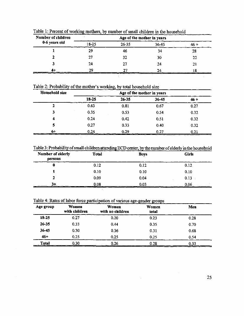
Table 1: Percent of working mothers, by number of small children in the householdNumber of children Age of the mother in years

0-6 years old 18-25 26-35 36-45 46 +

1 29 46 34 28

2 27 32 30 22

3 24 27 24 21

4+ 29 27 24 18

Table 2: Probability of the mother's working, by total household sizeHousehold size Age of the mother in years

18-25 26-35 36-45 46 +2 0.63 0.81 0.67 0.27

3 0.35 0.53 0.54 0.32

4 0.24 0.42 0.51 0.32

5 0.27 0.33 0.40 0.32

6+ 0.24 0.29 0.27 0.21

Table 3: Probability of small children attending ECD center, by the number ofelderly in the householdNumber of elderly Total Boys Girls

persons0 0.12 0.12 0.12

1 0.10 0.10 0.10

2 0.09 0.04 0.13

3+ 0.08 0.03 0.06

Table 4: Rates of labor force participation of various age-gender groupsAge group Women Women Women Men

with children with no children total18-25 0.27 0.20 0.23 0.28

26-35 0.33 0.44 0.35 0.7036-45 0.30 0.36 0.31 0.68

46+ 0.25 0.25 0.25 0.54

Total 0.30 0.26 0.28 0.53

25

,Table 5: Summary statistics for the dependent and explanatory variables.Mean STD Mean STD

Dependent variables Explanatory variables

Mother's work status 0.53 binary Nuclear family and other relatives 0.05 binary

Younger children in ECD center 0.18 binary Other types of households with children 0.07 binary

All children 8-16 years old are in 0.64 binary Agricultural income 0.03 0.09school')

All girls 8-16 years old are in school 2) 0.68 binary Nonagricultural income 0.12 0.86

All boys 8-16 years old are in school 3 0.71 binary Characteristics of the head

Other household members' work status 0.75 binary Age of household head 41.36 12.27

Explanatory variables Age of household head squared/100 18.60 11.85

Log of mother's wage 6.62 0.35 Gender of household head 0.80 binary

Log of other household members' wage 6.48 2.13 Education of the household head 0.02 0.13

Log of average expenditure on child care 4.42 0.24 Characteristics of the mother

Log of quality-adjusted cost of care 4.26 0.68 Mother's age 32.15 8.68

Lagged average wage per locality 6.87 0.47 Mother's age squared/lO0 11.08 63.95

Household characteristics Preschool education 0.01 binary

Total household size 6.84 2.81 Standard 1-8 (below CPE) 0.28 binary

Number of children 0-2 years old 0.70 0.67 Cert. of primary education (CPE) 0.15 binary

Number of children 3-5 years old 0.96 0.65 Junior sec. ed. (Form 1-4) 0.10 binary

Number of children 6-7 years old 0.72 0.65 Cert. of secondary ed. (KCSE) 0.07 binary

Number of children 8-12 years old 1.20 1.12 Trade test certificate 0.01 binary

Number of children 13-16 years old 0.63 0.88 Other postsecondary ed. 0.01 binary

Share of adult males in the household 0.16 0.10 University and above 0.00 binary

Share of adult females in the household 0.22 0.09 No education 0.37 binary

Share of elderly persons in the 0.01 0.05household' Average is calculated on a sample of households with children age 8-16.2) Average is calculated on a sample of households with girls age 8-16.3) Average is calculated on a sample of households with boys age 8-16.

26

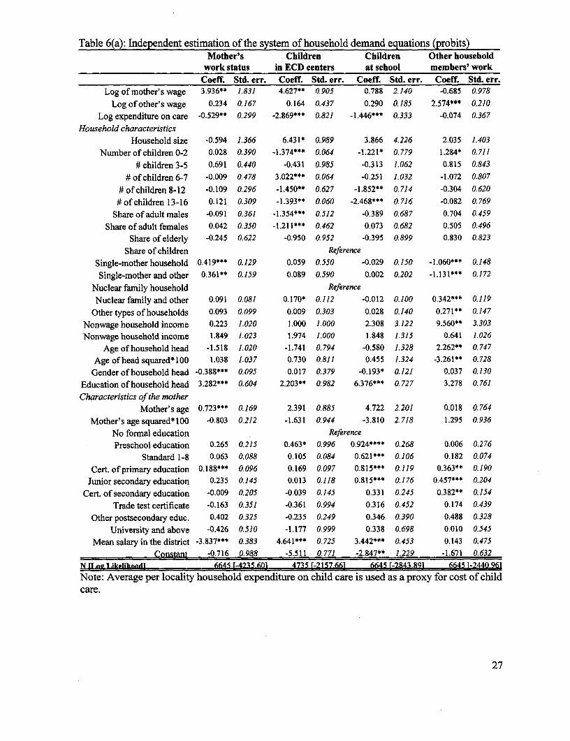
Table 6(a): Independent estimation of the system of household demand equations (probits)Mother's Children Children Other household

work status in ECD centers at school members' workCoeff. Std. err. Coeff. Std. err. Coeff. Std. err. Coeff. Std. err.

Log of mother's wage 3.936** 1.831 4.627** 0.905 0.788 2.140 -0.685 0.978

Log of other's wage 0.234 0.167 0.164 0.437 0.290 0.185 2.574*** 0.210

Log expenditure on care -0.529** 0.299 -2.869*** 0.821 -1.446*** 0.333 -0.074 0.367

Household characteristicsHousehold size -0.594 1.366 6.431* 0.989 3.866 4.226 2.035 1.403

Number of children 0-2 0.028 0.390 -1.374*** 0.064 -1.221* 0.779 1.284* 0.711

# children 3-5 0.691 0.440 -0.431 0.985 -0.313 1.062 0.815 0.843

# of children 6-7 -0.009 0.478 3.022*** 0.064 -0.251 1.032 -1.072 0.807

#of children 8-12 -0.109 0.296 -1.450** 0.627 -1.852** 0.714 -0.304 0.620

# of children 13-16 0.121 0.309 -1.393** 0.060 -2.468*** 0.716 -0.082 0.769

Share of adult males -0.091 0.361 -1.354*** 0.512 -0.389 0.687 0.704 0.459

Share of adult females 0.042 0.350 -1.211*** 0.462 0.073 0.682 0.505 0.496Share of elderly -0.245 0.622 -0.950 0.952 -0.395 0.899 0.830 0.823

Share of children Reference

Single-mother household 0.419*** 0.129 0.059 0.550 -0.029 0.150 -1.060*** 0.148

Single-mother and other 0.361** 0.159 0.089 0.590 0.002 0.202 -1.131*** 0.172

Nuclear family household ReferenceNuclear family and other 0.091 0.081 0.170* 0.112 -0.012 0.100 0.342*** 0.119

Other types of households 0.093 0.099 0.009 0.303 0.028 0.140 0.271** 0.147Nonwage household income 0.223 1.020 1.000 1.000 2.308 3.122 9.560** 3.303Nonwage household income 1.849 1.023 1.974 1.000 1.848 1.315 0.641 1.026

Age of household head -1.518 1.020 -1.741 0.794 -0.580 1.328 2.262** 0.747Age of head squared*l00 1.038 1.037 0.730 0.811 0.455 1.324 -3.261** 0.728

Gender of household head -0.388*** 0.095 0.017 0.379 -0.193* 0.121 0.037 0.130

Education of household head 3.282*** 0.604 2.203** 0.982 6.376*** 0.727 3.278 0.761

Characteristics of the motherMother's age 0.723*** 0.169 2.391 0.885 4.722 2.201 0.018 0.764

Mother's age squared* 100 -0.803 0.212 -1.631 0.944 -3.810 2.718 1.295 0.936

No formal education ReferencePreschool education 0.265 0.215 0.463* 0.996 0.924**** 0.268 0.006 0.276

Standard 1-8 0.063 0.088 0.105 0.084 0.621*** 0.106 0.182 0.074

Cert. of primary education 0.188*** 0.096 0.169 0.097 0.815*** 0.119 0.363** 0.190Junior secondary education 0.235 0.145 0.013 0.118 0.815*** 0.176 0.457*** 0.204

Cert. of secondary education -0.009 0.205 -0.039 0.145 0.331 0.245 0.382** 0.154

Trade test certificate -0.163 0.351 -0.361 0.994 0.316 0.452 0.174 0.439Other postsecondary educ. 0.402 0.325 -0.235 0.249 0.346 0.390 0.488 0.328

University and above -0.426 0.510 -1.177 0.999 0.338 0.698 0.010 0.545Mean salary in the district -3.837*** 0.383 4.641*** 0.725 3.442*** 0.453 0.143 0.475

Constant -0.716 0.988 -5.511 0.771 -2.847** 1.229 -1.671 0.632N 11T g 1 .ikPlihnndl 6645 1-4235 601 4735 [-2157 661 6645 f-2843-89] 6645 [-24402961Note: Average per locality household expenditure on child care is used as a proxy for cost of childcare.

27

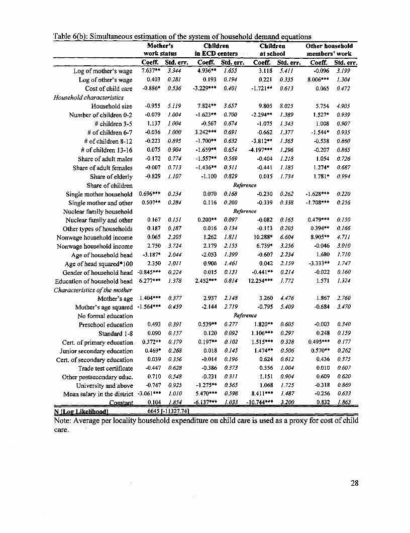
Table 6(b): Simultaneous estimation of the system of household demand equationsMother's Children Children Other household

work status in ECD centers at school members' workCoeff. Std. err. Coeff. Std. err. Coeff. Std. err. Coeff. Std. err.

Log of mother's wage 7.637** 3.344 4.936** 1.655 3.118 5.411 -0.096 3.199Log of other's wage 0.403 0.281 0.193 0.194 0.221 0.335 8.006*** 1.304

Cost of child care -0.886* 0.536 -3.229*** 0.401 -1.721** 0.613 0.065 0.472

Household characteristicsHousehold size -0.955 5.119 7.824** 3.657 9.805 8.025 5.754 4.905

Number of children 0-2 -0.079 1.004 -1.623** 0.700 -2.294** 1.389 1.527* 0.939# children 3-5 1.137 1.004 -0.567 0.674 -1.075 1.343 1.008 0.907

#of children 6-7 -0.036 1.000 3.242*** 0.691 -0.662 1.377 -1.544* 0.935# of children 8-12 -0.223 0.895 -1.700** 0.632 -3.812** 1.365 -0.538 0.860

# of children 13-16 0.075 0.904 -1.659* 0.654 -4.197*** 1.296 -0.207 0.865Share of adult males -0.172 0.774 -1.557** 0.569 -0.404 1.218 1.054 0.726

Share of adult females -0.007 0.713 -1.436** 0.511 -0.441 1.185 1.274* 0.687Share of elderly -0.829 1.107 -1.100 0.829 0.015 1.734 1.781* 0.994

Share of children ReferenceSingle mother household 0.696*** 0.234 0.070 0.168 -0.230 0.262 -1.628*** 0.220Single mother and other 0.507** 0.284 0.116 0.200 -0.339 0.338 -1.708*** 0.256

Nuclear family household ReferenceNuclear family and other 0.167 0.151 0.200** 0.097 -0.082 0.165 0.479*** 0.150

Other types of households 0.187 0.187 0.016 0.134 -0.113 0.205 0.394** 0.166Nonwage household income 0.065 2.205 1.262 1.811 10.288* 6.604 8.905** 4.711Nonwage household income 2.750 3.724 2.179 2.155 6.739* 3.256 -0.046 3.010

Age of household head -3.187* 2.044 -2.053 1.399 -0.607 2.234 1.680 1.710Age of head squared* 100 2.350 2.011 0.906 1.461 0.042 2.159 -3.333** 1.747

Gender of household head -0.845*** 0.224 0.015 0.131 -0.441** 0.214 -0.022 0.160Education of household head 6.277*** 1.378 2.452*** 0.814 12.254*** 1.772 1.571 1.324

Characteristics of the motherMother's age 1.404*** 0.377 2.937 2.148 3.260 4.476 1.867 2.760

Mother's age squared -1.564*** 0.459 -2.144 2.719 -0.795 5.409 -0.684 3.470No formal education ReferencePreschool education 0.493 0.391 0.539** 0.277 1.820** 0.605 -0.003 0.340

Standard 1-8 0.090 0.157 0.120 0.092 1.106*** 0.297 0.248 0.159Cert. of primary education 0.372** 0.179 0.197** 0.102 1.515*** 0.328 0.495*** 0.177

Junior secondary education 0.469* 0.268 0.018 0.145 1.474** 0.506 0.570** 0.262Cert. of secondary education 0.039 0.356 -0.014 0.196 0.624 0.612 0.436 0.375

Trade test certificate -0.447 0.628 -0.386 0.373 0.356 1.004 0.010 0.607Other postsecondary educ. 0.710 0.548 -0.231 0.311 1.151 0.904 0.609 0.620

University and above -0.747 0.925 -1.275** 0.565 1.068 1.725 -0.318 0.869Mean salary in the district -3.061*** 1.010 5.470*** 0.598 8.411*** 1.487 -0.256 0.633

Constant 0.104 1.854 -6.137*** 1.033 -10.744*** 3.200 0.832 1.863N [Log Likelihood] 6645 [-11327.741

Note: Average per locality household expenditure on child care is used as a proxy for cost of childcare.

28

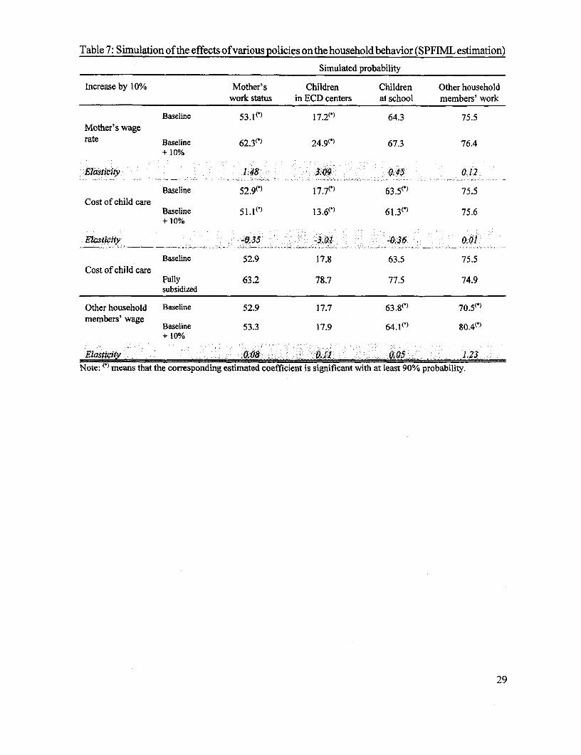
Table 7: Simulation of the effects of various policies on the household behavior (SPFIML estimation)

Simulated probability

Increase by 10% Mother's Children Children Other householdwork status in ECD centers at school members' work

Baseline 53.1() 17.2( ) 64.3 75.5Mother's wagerate Baseline 62.3(*) 24.9(*) 67.3 76.4

+ 10%

Elasticity 1.48 3.09 0.45 0.12

Baseline 52.9(*) 17.7( ) 63.5(*) 75.5Cost of child care

Baseline 51.1(') 13.6(*) 61.3(*) 75.6+ 10%

Elasticity -0.35 -3.01 -0.36 0.01

Baseline 52.9 17.8 63.5 75.5Cost of child care

Fully 63.2 78.7 77.5 74.9subsidized

Other household Baseline 52.9 17.7 63.8°* 70.5°'

members' wage Baseline 53.3 17.9 64.1(*) 80.4("+ 10%

Elaticiy 0.08 .011 0.05 1.23Note: ° means that the corresponding estimated coefficient is significant with at least 90% probability.

29

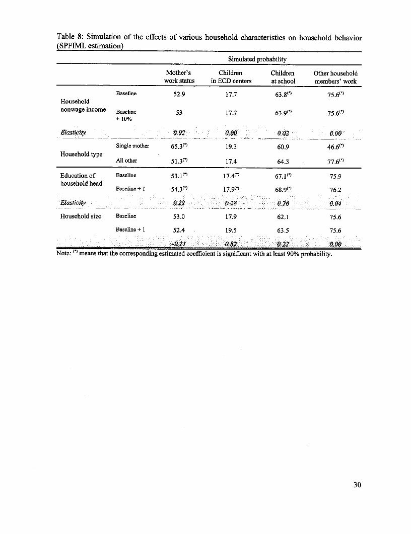
Table 8: Simulation of the effects of various household characteristics on household behavior(SPFIML estimation)

Simulated probability

Mother's Children Children Other householdwork status in ECD centers at school members' work

Baseline 52.9 17.7 63.8(*) 75.61*Householdnonwage income Baseline 53 17.7 63.9( ) 75.6("

+ 10%

ElIJiy 0Q2 0.00 0.02 :f A A0.00

Single mother 65.3( ) 19.3 60.9 46.6(7Household type

All other 51.3(') 17.4 64.3 77.6(*

Education of Baseline 53.1( ) 17.4() 67.1(*) 75.9household head

Baseline + 1 54.3(') 17.9(*) 68.9( ) 76.2: . . f S 0 8 . 0 : .

Elasticity 0.22 0.0; 0.2 0,04

Household size Baseline 53.0 17.9 62.1 75.6

Baseline + 1 52.4 19.5 63.5 75.6

E0.22 0 00Note: ° means that the corresponding estimated coefficient is significant with at least 90% probability.

30

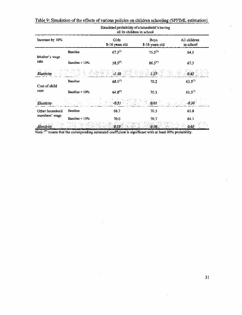
Table 9: Simulation of the effects of various policies on children schooling (SPFIML estimation)

Simulated probability of a household's havingall its children in school

Increase by 10% Girls Boys All children8-16 years old 8-16 years old in school

Baseline 67.3(') 75.5(') 64.3Mother's wagerate Baseline + 10% 58.5( ) 86.5( ) 67.3

Elasticity -1.S 1,27 0. 4'

Baseline 68.1(') 70.2 63.5()Cost of childcare Baseline + 10%/o 64.8( ) 70.3 61.3()

Elasticity -0.51 0`01 -0.36

Other household Baseline 68.7 70.3 63.8members' wage Bsln 0

member e Baseline+ IO% 70.0 70.7 64.1

Elasticit a 9 - 0.()6 0,,Note: (') means that the corresponding estimated coefficient is significant with at least 900/O probability.

31

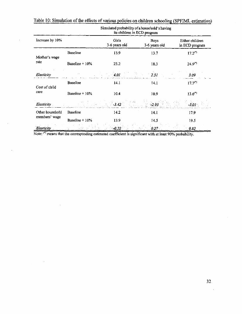
Table 10: Simulation of the effects of various policies on children schooling (SPFIML estimation)

Simulated probability ofa household's havingits children in ECD programn

Increase by 10% Girls Boys Either children3-6 years old 3-6 years old in ECD program

Baseline 13.9 13.7 17.2('Mother's wagerate Baseline + 10% 23.2 18.3 24.9('

Elasticity 0 f 4.RJ ;01f fO 2z5V 3.09

Baseline 14.1 14.1 17.7°')Cost of childcare Baseline + 10% 10.4 10.9 13.6°*

Elasticity __ -3.42 -402.93 . 3.

Other household Baseline 14.2 14.1 17.9members' wage

Baseline + 10% 13.9 14.5 19.5

Note: ° means that the corresponding estimated coefficient is significant with at least 90% probability.

32

Appendix

In the SPFIML estimation the following functional forms were assumed in estimating the probabilityweights Pk, Pi, and P,,, and the points of support for factors VI, V2, and V 3 :

P.. exp(bmn) _ n=1,...,N-1 P.in = 11+ exp(bm) 1+ exp(bmn)

Vmn =exp(amn ) n = 2,..., N - I Vm. = O; VmN l

1 + exp(amn)

33

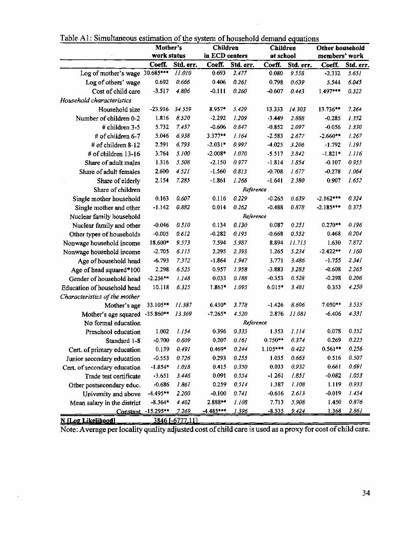
Table Al: Simultaneous estimation of the system of household demand equationsMother's Children Children Other household

work status in ECD centers at school members' work

Coeff. Std. err. Coeff. Std. err. Coeff. Std. err. Coeff. Std. err.Log of mother's wage 30.685*** 11.010 0.693 2.477 0.080 9.558 -2.332 5.651

Log of others' wage 0.692 0.666 0.406 0.261 0.798 0.639 5.544 6045

Cost of child care -3.517 4.806 -0.111 0.260 -0.607 0.443 1.497*** 0.322

Household characteristicsHousehold size -23.916 34.559 8.957* 5.429 13.333 14.303 13.736** 7.264

Number of children 0-2 1.816 8.520 -2.292 1.209 -3.449 2.888 -0.285 1.352

# children 3-5 5.732 7.437 -0.606 0.847 -0.852 2.097 -0.056 1.330#of children 6-7 5.046 6938 3.377** 1.164 -2.583 2.677 -2.660** 1.267

#ofchildren8-12 2.591 6.793 -2.031* 0.997 -4.025 3.206 -1.792 1.191

#ofchildren 13-16 3.764 5.100 -2.008* 1.070 -5.517 3.842 -1.821* 1.116Share of adult males 1.316 5.508 -2.150 0.977 -1.814 1.854 -0.107 0.955

Share of adult females 2.600 4.521 -1.560 0.813 -0.708 1.677 -0.278 1.064Share of elderly 2.154 7.285 -1.861 1.266 -1.641 2.380 0.907 1.652

Share of children ReferenceSingle mother household 0.163 0.607 0.116 0.229 -0.265 0.639 -2.162*** 0.324Single mother and other -1.142 0.882 0.014 0.262 -0.488 0.878 -2.185*** 0.375

Nuclear family household ReferenceNuclear family and other -0.046 0.510 0.134 0.130 0.087 0.251 0.270** 0.196

Other types of households -0.005 0.612 -0.282 0.195 -0.668 0.552 0.468 0.204Nonwage household income 18.600* 9.573 7.594 5.987 8.894 11.715 1.630 7.872Nonwage household income -2.705 6115 2.295 2.393 1.265 5.234 -2.422** 1.160

Age of household head -6.793 7.372 -1.864 1.947 3.771 3.486 -1.755 2.341Age of head squared*100 2.298 6525 0.957 1.958 -3.883 3.283 -0.608 2.265

Gender of household head -2.256** 1.148 0.033 0.188 -0.353 0.528 -0.298 0.206

Education of household head 10.118 6325 1.863* 1.095 6.015* 3.481 0.353 4.250

Characteristics of the motherMother's age 33.105** 11.387 6.430* 3.778 -1.426 8.606 7.050** 3.535

Mother's age squared -35.860** 13.369 -7.265* 4.520 2.876 11.081 -6.406 4.331No fonnal education ReferencePreschool education 1.002 1.154 0.396 0.333 1.353 1.114 0.078 0.352

Standard 1-8 -0.700 0.609 0.207 0.161 0.750** 0.374 0.269 0.225Cert. of primary education 0.139 0.491 0.469* 0.244 1.105*** 0.422 0.561** 0.256

Junior secondary education -0.553 0.726 0.293 0.255 1.035 0.663 0.516 0.507Cert. of secondary education -1.854* 1.018 0.415 0.350 0.033 0.932 0.661 0.691

Trade test certificate -3.651 3.446 0.091 0.554 -1.261 1.851 -0.082 1.053Other postsecondary educ. -0.686 1.861 0.259 0.514 1.387 1.108 1.119 0.933

University and above -4.495** 2.200 -0.100 0.741 -0.616 2.613 -0.019 1.454Mean salary in the district -8.364* 4.402 2.888** 1.108 7.713 5.908 1.450 0.876

Constant -15.295** 7.269 -4.485*** 1.396 -8.535 9.424 1.368 2.861

N [Log Likelihood] 3846 [-6777.1 11Note: Average per locality quality adjusted cost of child care is used as a proxy for cost of child care.

34

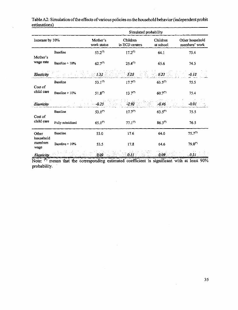
Table A2: Simulation ofthe effects of various policies on the household behavior (independent probitestimations)

Simulated probability

Increase by 10% Mother's Children Children Other householdwork status in ECD centers at school members' work

Baseline 53.2(') 17.2(') 64.1 75.4Mother'swage rate Baseline + 10% 62.7(*) 25.4(*) 65.6 74.5

Elasticity 1.52 3.23 0.23 -0.12

Baseline 53.1( 17.7(*l 63.5(*) 75.5Cost ofchild care Baseline + 10% 51.8(*) 13.7(*) 60.7(') 75.4

Elasticity -0.25 -2.92 -0.46 -0.01

Baseline 53.1('- 17.7(" 63.5( ) 75.5Cost ofchild care Fully subsidized 65.1( ) 77.1(') 86.3(*) 76.5

Other Baseline 53.0 17.6 64.0 75.7(*)householdmembers Baseline + 10% 53.5 17.8 64.6 79.8wage

.lasticity 0.09 0.11 0.09 0.51Note: (*) means that the corresponding estimated coefficient is significant with at least 90%probability.

35

Policy Research Working Paper Series

ContactTitle Author Date for paper

WPS2352 How Stronger Patent Protection in Carsten Fink May 2000 L. TabadaIndia Might Affect the Behavior 36896of Transnational PharmaceuticalIndustries

WPS2353 The Sao Mateus-Jabaquara Jorge Rebelo May 2000 S. Van VeldhuizenTrolleybusway Concession in Brazil Pedro Machado 38722

WPS2354 When the Bureaucrats Move out of Yi Chen May 2000 M. YafiBusiness: A Cost-Benefit Ishac Diwan 34649Assessment of Labor Retrenchmentin China

WPS2355 Greed and Grievance in Civil War Paul Collier May 2000 A. Kitson-WaltersAnke Hoeffler 33712

WPS2356 Bureaucratic Delegation and Political Philip Keefer June 2000 P. Sintim-AboagyeInstitutions: When Are Independent David Stasavage 37644Central Banks Irrelevant?

WPS2357 Evaluating Carbon Offsets from Kenneth M. Chomitz June 2000 J. AncrumForestry and Energy Projects: 33512How Do They Compare?

WPS2358 Why Infrastructure Financing Daniela Klingebiel June 2000 M. SalehiFacilities Often Pall Short of Their Jeff Ruster 37157Objectives

WPS2359 Reducing Carbon Dioxide Emissions Will Martin June 2000 L. TabadaThrough Joint Implementation of 36896Projects

WPS2360 Corruption and the Composition of Beata K. Smarzynska June 2000 H. SladovichForeign Direct Investment: Shang-Jin Wei 37698Firm-Level Evidence

WPS2361 The Welfare Effects of Private Sector George Clarke June 2000 H. SladovichParticipation in Guinea's Urban Water Claude M6nard 37698Supply Ana Maria Zuluaga

WPS2362 A Transitory Regime: Water Supply Claude M6nard June 2000 H. SladovichIn Conakry, Guinea George Clarke 37698

WPS2363 Would Collective Action Clauses Barry Eichengreen June 2000 S. KpundehRaise Borrowing Costs? An Update Ashoka Mody 39591and Additional Results

WPS2364 Perverse Effects of a Ratings- Patrick Honohan June 2000 A. YaptencoRelated Capital Adequacy System 38526

Policy Research Working Paper Series

ContactTitle Author Date for paper

WPS2365 Leading Indicator Project: Lithuania Stephen S. Everhart June 2000 M. GellerRobert Duval-Hernandez 85155

WPS2366 Fiscal Constraints, Collection Costs, Keiko Kubota June 2000 L. Tabadaand Trade Policies 36896

WPS2367 Gender, Poverty, and Nonfarm Constance Newman June 2000 M. ClarkeEmployment in Ghana and Uganda Sudharshan Canagarajan 31752

WPS2368 Seeds of Corruption: Do Market Harry G. Broadman June 2000 S. CraigInstitutions Matter? Francesca Racanatini 33160

WPS2369 How the Proposed Basel Guidelines Giovanni Ferri June 2000 E. MekhovaOn Rating-Agency Assessments Li-Gang Liu 85984Would Affect Developing Countries Giovanni Majnoni

WPS2370 A New Model for Market-Based Marcelo Giugale June 2000 M. GellerRegulation of Subnational Borrowing: Adam Korobow 85155The Mexican Approach Steven Webb

WPS2371 Shock Persistence and the Choice Marcelo Giugale June 2000 M. Gellerof Foreign Exchange Regime: An Adam Korobow 85155Empirical Note from Mexico

WPS2372 Financial Openness, Democracy, Mansoor Dailami June 2000 W. Nedrowand Redistributive Policy 31585

WPS2373 Reciprocity across Modes of Supply Aaditya Mattoo June 2000 L. Tabadain the World Trade Organization: Marcelo Olarreaga 36896A Negotiating Formula

WPS2374 Should Credit Be Given for Aaditya Mattoo June 2000 L. TabadaAutonomous Liberalization in Marcelo Olarreaga 36896Multilateral Trade Negotiations?

WPS2375 Asset Distribution, Inequality, Klaus Deininger June 2000 M. Fernandezand Growth Pedro Olinto 33766