The Effect of Clay Content and Iron Oxyhydroxide Coatings on the Dielectric Properties of Quartz Sand

Michael V. Cangialosi

Thesis submitted to the faculty of the Virginia Polytechnic Institute and State University in partial fulfillment of the requirements for the degree of

Master of Science in

Geosciences

Patricia M. Dove Chester J. Weiss

Donald J. Rimstidt

April 27, 2012 Blacksburg, VA

Keywords: Time Domain Reflectometry, Dielectric Constant, Volumetric Water Content, Kaolin Clay, Iron Oxyhydroxide Coatings

The Effect of Clay Content and Iron Oxyhydroxide Coatings on the Dielectric Properties of Quartz Sand

Michael V. Cangialosi

ABSTRACT

Dielectric constant is a physical property of soil that is often measured using non-invasive geophysical techniques in subsurface characterization studies. A proper understanding of dielectric responses allows investigators to make measurements that might otherwise require more invasive and/or destructive methods. Previous studies have suggested that dielectric models could be refined by accounting for the contributions of different types of mineral constituents that affect the ratio and properties of bound and bulk water. This study tested the hypothesis that the dielectric responses of porous materials are mineral-specific through differences in surface area and chemistry. An experimental design was developed to test the dielectric behavior of pure quartz sand (Control), quartz sand/kaolin clay mixtures and ferric oxyhydroxide coated quartz sand. Results from the experiments show that the dielectric responses of quartz-clay and iron oxyhydroxide modified samples are not significantly different from the pure quartz Control. Increasing clay content in quartz sands leads to a vertical displacement between fitted polynomials. The results suggest that the classic interpretation for the curvature of dielectric responses appears to be incorrect. The curvature of dielectric responses at low water contents appears to be controlled by unknown parameters other than bound water. A re-examination of the experimental procedure proposed in this study and past studies shows that a properly designed study of bound water effects on dielectric responses has not yet been conducted.

iii

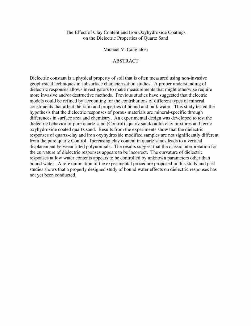
Table of Contents Table of Contents…………………………………………………………….………………….iii List of Figures……………..………………………………….………………...………………..iv List of Tables.……………………………………………………………………...………..…...vi List of Appendices…………………………………………………………………………..….vii 1. Introduction: Near Surface Characterization and Dielectric Behavior Models................1

1.1 The Critical Zone and Subsurface Characterization………………………………1 1.2 Invasive Characterization Techniques…………………………………………….2 1.3 Non-Invasive Geophysical Characterization……..…………………………….…3 1.4 Dielectric Constant of Soils…………..…………...…………………………...….5 1.5 Extending Dielectric Behavior Models……………………...……….…………....6

2. Background: Modeling the Dielectric Behavior of Unsaturated Soils…...…..………….12

2.1 Traditional Dielectric Behavior Models for TDR………............................……..12 3. Background: Dielectrics and Porous Media…………..………………….…………….....20

3.1 An Introduction to Dielectric Constants………………………………………....20 3.2 Estimating Dielectric Constant using TDR……………………………...……….22

4. Materials and Methods……………………………………………….……………...…..…27

4.1 Introduction………………………………………………………………………27 4.2 TDR System Materials…………………………………………………………...29 4.3 Sample Apparatus Materials………………………………………..............……29 4.4 Experimental Procedure for the Control and kaolin Clay/Quartz Sand

Mixtures.................................................................................................................31 4.5 Experimental Procedure for Iron Oxyhydroxide Coated Quartz Grains…..….....33

5. Results and Discussion……………………………………………………………….……..35

5.1 Quartz Sand/kaolin Clay Observations…….…………………………………….35 5.2 Quartz Sand Control Analysis…………………………………………………...36 5.3 Quartz Sand/kaolin Clay Analysis………………………………………….……36 5.4 Iron Oxyhydroxide Observations…………………………………………..…….48 5.5 Iron Oxyhydroxide Results……………………………………………………....49

6. Summary……………………………………………………………….…………………....55

References……………………………..……………………………………………………...…57

iv

List of Figures Figure 1 Calibration model for the relationship between dielectric constant and volumetric water content derived by Topp et al., (1980)……………………………………………..…………...…8 Figure 2. The curvature of the polynomial representing the relationship between dielectric constant and volumetric water content is a function of the dielectric constants of bound versus bulk water..…………………………………….…………………………………………………..9 Figure 3. Quantitative illustration of bound versus bulk water in the pore space of porous materials. Wilting point is defined as the water content at which the soil tension is approximately 15 bars and it becomes difficult for plants to remove water. Field capacity is defined as the water content at which the soil tension is about 1/3 bars and water is able to flow with gravity. ….………………………………………………………………………………….11 Figure 4 Calibration models for the relationship between dielectric constant and volumetric water content that are reported in Topp et al. (1980) and Ledieu et al. (1986)………………….16 Figure 5 Water molecules with no orientation (left) due to thermal motion and (right) the organization of water molecules in the presence of an electric field. Figure based on Robinson et al., (2003). …………………………………………………………………...…………………..21 Figure 6 Illustration of the probe component of the TDR100 waveguide that is inserted into the study media for electromagnetic wave propagation. Figure is not to scale……………..………25 Figure 7. Schematic of a typical waveform recorded analyzed by the TDR100 with three key points labeled A, B and C (figure adapted from TDR100 instructional manual, Campbell Scientific). The waveform before point A represents the coaxial cable before the probe head. Point A represents the transition from the coaxial cable to the probe. The rapid change in reflection coefficient after point A is due to the change in impedance from the coaxial cable to the probe. Point B represents the point where the probe is no longer insulated by the probe head and makes contact with the study media. Point C represents the end of the probe. Apparent Length (La), the parameter calculated from the waveform and used to calculate the apparent dielectric constant, is the distance between points B and C……………………………………..26 Figure 8 Illustration of the experimental design. The TDR probe is connected to the TDR100, power source and computer running PCTDR software. The sample apparatus is connected to the solution trap flask and vacuum pump as well as an air bubbler to control humidity…………....28 Figure 9 The primary sample holder is shown in this illustration of the sample apparatus that was constructed for this study to measure the dielectric responses of quartz and clay mixtures with different physical and chemical parameters……………………………………………...…30 Figure 10 (A) Dielectric constant vs. volumetric water content data for 0% clay content (control). (B) Goodness of fit plot showing the absolute and relative error with changing water content. On the relative error axis 0.08 corresponds to 8%. The data shown is from the 0% clay treatment shown in Appendix A………..………………………………………………….….…39 Figure 11 (A) Dielectric constant vs. volumetric water content data for 2% clay content. (B) Goodness of fit plot showing the absolute and relative error with changing water content. On the relative error axis 0.08 corresponds to 8%. The data shown is from the 2% clay treatment shown in Appendix A……………………………………………………………………...…………….40 Figure 12(A) Dielectric Constant vs. volumetric water content data for 4% clay content. (B) Goodness of fit plot showing the absolute and relative error with changing water content. On the relative error axis 0.08 corresponds to 8%. The data shown is from the 4% clay treatment shown in Appendix A………………………………………………………………...………………….41

v

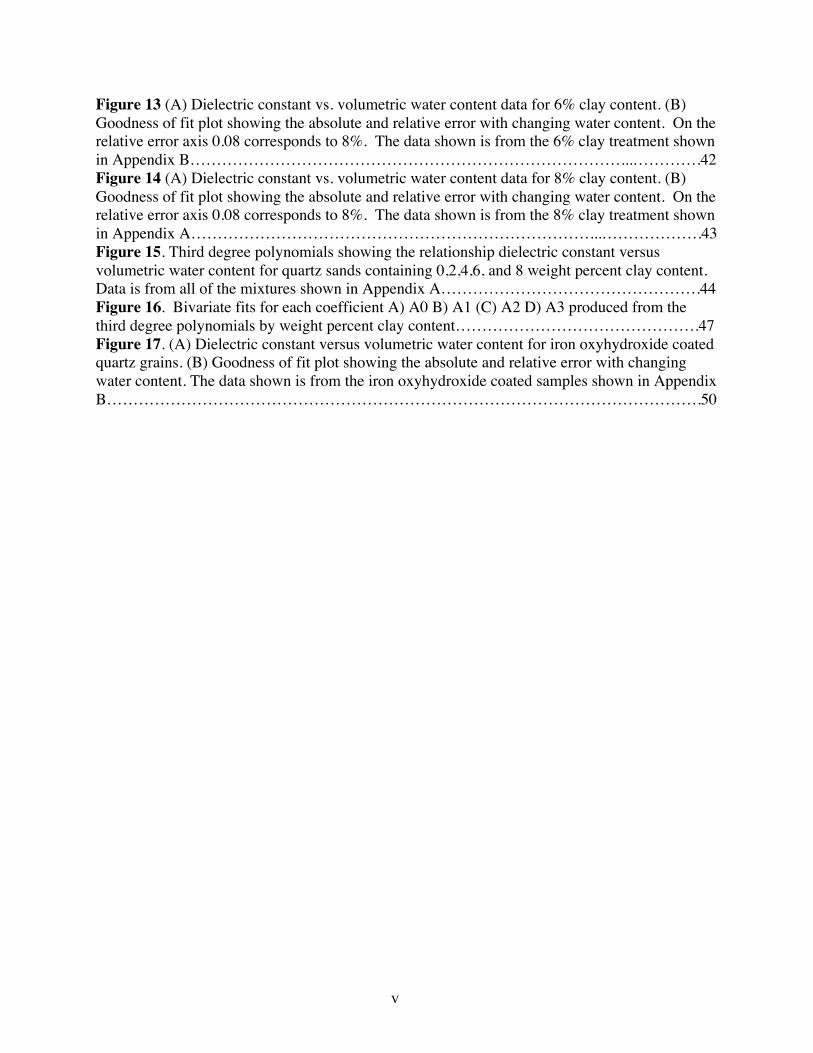
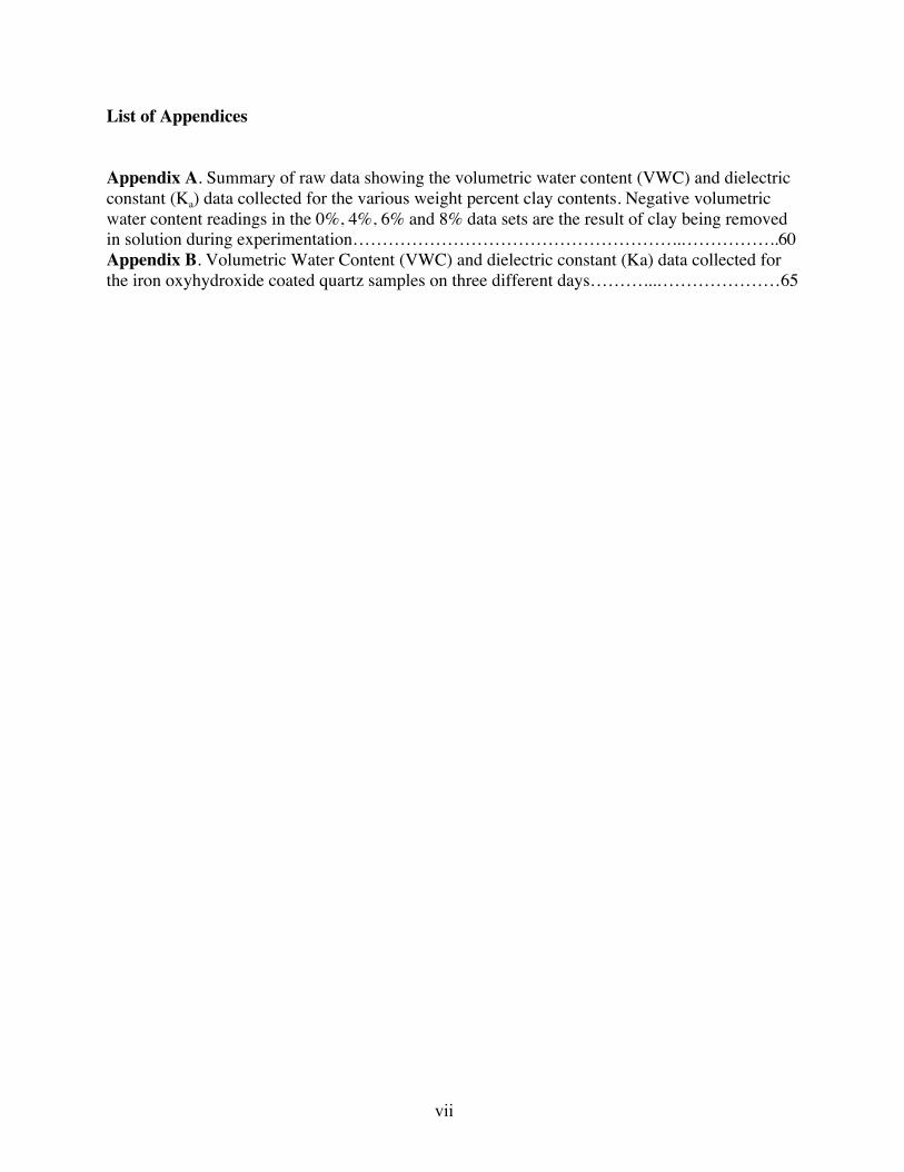
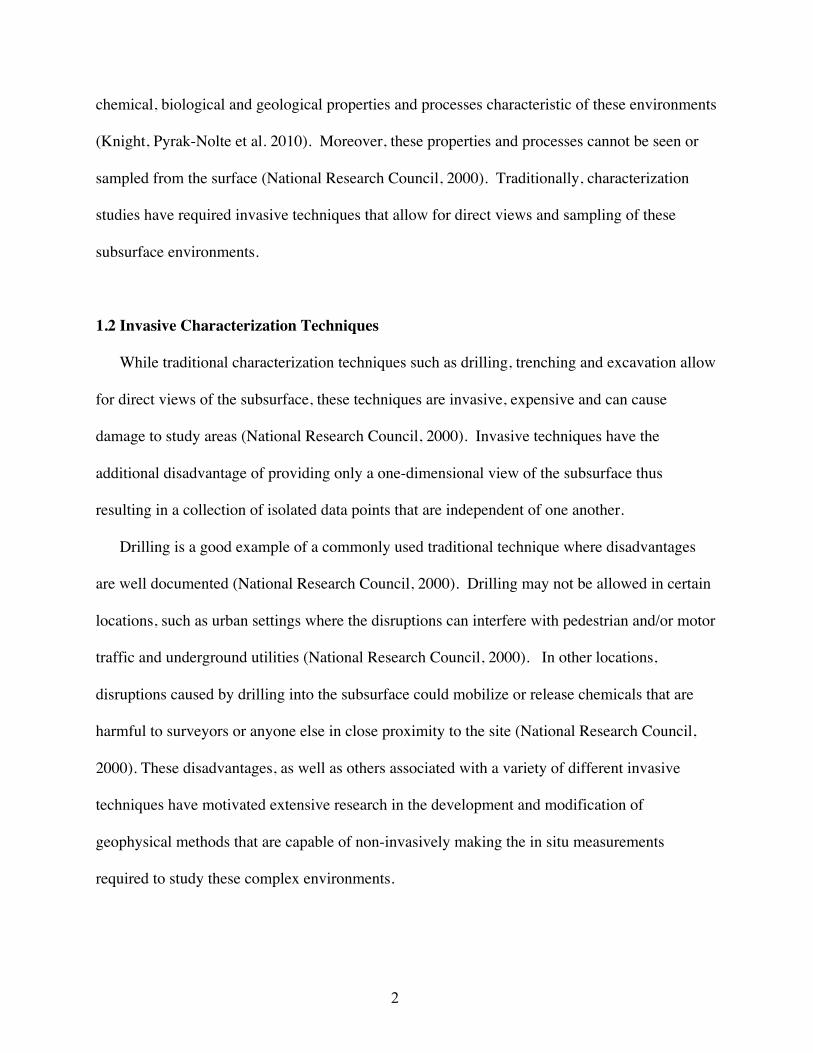
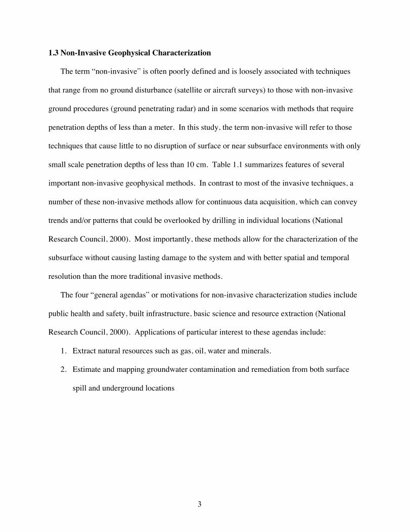
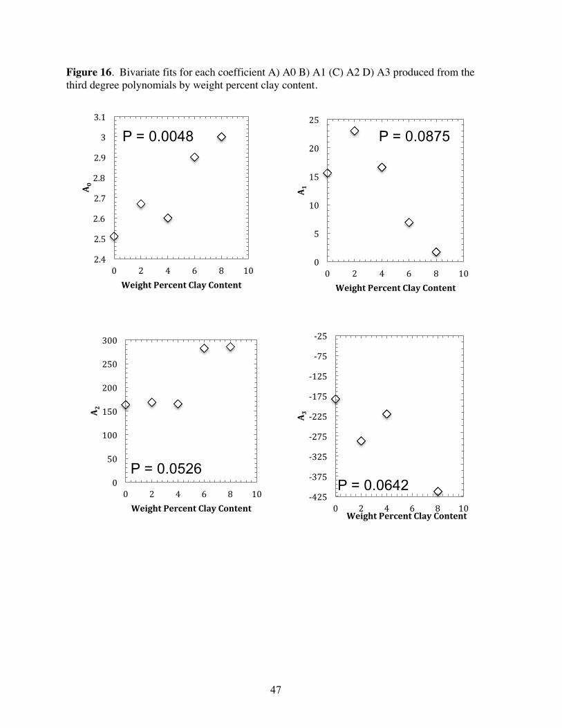
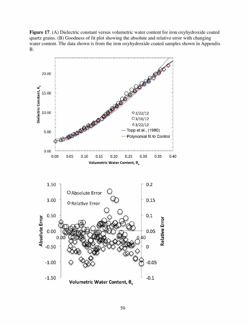
Figure 13 (A) Dielectric constant vs. volumetric water content data for 6% clay content. (B) Goodness of fit plot showing the absolute and relative error with changing water content. On the relative error axis 0.08 corresponds to 8%. The data shown is from the 6% clay treatment shown in Appendix B………………………………………………………………………...………….42 Figure 14 (A) Dielectric constant vs. volumetric water content data for 8% clay content. (B) Goodness of fit plot showing the absolute and relative error with changing water content. On the relative error axis 0.08 corresponds to 8%. The data shown is from the 8% clay treatment shown in Appendix A…………………………………………………………………...……………….43 Figure 15. Third degree polynomials showing the relationship dielectric constant versus volumetric water content for quartz sands containing 0,2,4,6, and 8 weight percent clay content. Data is from all of the mixtures shown in Appendix A………………………………………….44 Figure 16. Bivariate fits for each coefficient A) A0 B) A1 (C) A2 D) A3 produced from the third degree polynomials by weight percent clay content……………………………………….47 Figure 17. (A) Dielectric constant versus volumetric water content for iron oxyhydroxide coated quartz grains. (B) Goodness of fit plot showing the absolute and relative error with changing water content. The data shown is from the iron oxyhydroxide coated samples shown in Appendix B………………………………………………………………………………………………….50

vi

List of Tables Table 1 Summary of non-invasive geophysical techniques used for subsurface characterization (adapted from National Research Council, 2000)……………………………………………..…..4 Table 2. Dielectric Constants of major soil constituents (Davis et al., 1989; Lucius et al., 1989; Olhoeft et al., 1989; Atkins, P.W., 1979)…………………………………………………………7 Table 3. Summary of the geochemical index properties for the Kaolin clay used in the quartz sand/kaolin clay mixtures. Activity (A) = PI (%) divided by the % clay fraction, where PI is the plasticity index from an Atterberg limits test. % Clay fraction is the percentage of the whole sample that is smaller than 2 microns (Dove, pers. comm., 2012)…………...32 Table 4. Summary of the polynomials produced from least square regressions for collected dielectric constant versus volumetric water content data at 0-8 weight percent clay contents. Polynomials are shown in the form Ka = A0 + A1θ + A2 θ2 +A3θ3……………………………....38

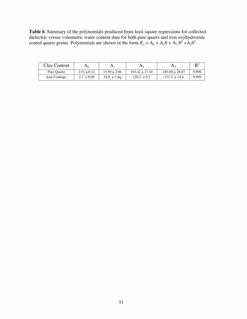
Table 5. P-values from T-tests used to evaluate the statistical significance of weight percent clay on each coefficient in the third degree polynomials that quantify the relationship between dielectric constant and volumetric water content………………………………………………...46 Table 6. Summary of the polynomials produced from least square regressions for collected dielectric versus volumetric water content data for both pure quartz and iron oxyhydroxide coated quartz grains. Polynomials are shown in the form Ka = A0 + A1θ + A2 θ2 +A3θ3………..51

vii

List of Appendices Appendix A. Summary of raw data showing the volumetric water content (VWC) and dielectric constant (Ka) data collected for the various weight percent clay contents. Negative volumetric water content readings in the 0%, 4%, 6% and 8% data sets are the result of clay being removed in solution during experimentation………………………………………………..……………..60 Appendix B. Volumetric Water Content (VWC) and dielectric constant (Ka) data collected for the iron oxyhydroxide coated quartz samples on three different days………...…………………65

1

1. Introduction to Near Subsurface Characterization and Dielectric Behavior Models

1.1 The Critical Zone and Subsurface Characterization

The Critical Zone, as defined by the National Research Council, consists of the surface and

near subsurface environments that is home to almost all terrestrial forms of life (National

Research Council, 2000). This zone, extending from “the upper limits of growing vegetation

down to lowest limits of groundwater”, is the “reactor” that houses the chemical reactions

required to provide the nutrients and energy necessary to sustain terrestrial life on earth

(Brantley, 2007). The population relies on the critical zone for more resources than just those

required for basic survival such as food and water. Societies are reliant on the critical zone for

the mineral and energy resources that are critical to economies, for the support of built

infrastructures, and for the storage of nearly every type of human waste (National Research

Council, 2000). Increased populations and expanding economies continue to increase the

demands that are put on the critical zone and are thus motivating the growing efforts to

understand the properties, behavior and responses of this zone to human perturbations. One of

the ways to meet these challenges is through proper characterization techniques. These allow us

to gather information that establishes a baseline about the critical zone and predicts responses to

human perturbations over time.

The terrestrial subsurface is a heterogeneous environment composed of the porous and

consolidated earth materials that include soil, sediments and rock. Each of these medias exhibit

a number of different properties and undergo environment-specific processes that vary across

spatial and temporal scales (National Research Council, 2000). One reason the characterization

of these complex environments is extremely difficult is because of the inter-dependent physical,

2

chemical, biological and geological properties and processes characteristic of these environments

(Knight, Pyrak-Nolte et al. 2010). Moreover, these properties and processes cannot be seen or

sampled from the surface (National Research Council, 2000). Traditionally, characterization

studies have required invasive techniques that allow for direct views and sampling of these

subsurface environments.

1.2 Invasive Characterization Techniques

While traditional characterization techniques such as drilling, trenching and excavation allow

for direct views of the subsurface, these techniques are invasive, expensive and can cause

damage to study areas (National Research Council, 2000). Invasive techniques have the

additional disadvantage of providing only a one-dimensional view of the subsurface thus

resulting in a collection of isolated data points that are independent of one another.

Drilling is a good example of a commonly used traditional technique where disadvantages

are well documented (National Research Council, 2000). Drilling may not be allowed in certain

locations, such as urban settings where the disruptions can interfere with pedestrian and/or motor

traffic and underground utilities (National Research Council, 2000). In other locations,

disruptions caused by drilling into the subsurface could mobilize or release chemicals that are

harmful to surveyors or anyone else in close proximity to the site (National Research Council,

2000). These disadvantages, as well as others associated with a variety of different invasive

techniques have motivated extensive research in the development and modification of

geophysical methods that are capable of non-invasively making the in situ measurements

required to study these complex environments.

3

1.3 Non-Invasive Geophysical Characterization

The term “non-invasive” is often poorly defined and is loosely associated with techniques

that range from no ground disturbance (satellite or aircraft surveys) to those with non-invasive

ground procedures (ground penetrating radar) and in some scenarios with methods that require

penetration depths of less than a meter. In this study, the term non-invasive will refer to those

techniques that cause little to no disruption of surface or near subsurface environments with only

small scale penetration depths of less than 10 cm. Table 1.1 summarizes features of several

important non-invasive geophysical methods. In contrast to most of the invasive techniques, a

number of these non-invasive methods allow for continuous data acquisition, which can convey

trends and/or patterns that could be overlooked by drilling in individual locations (National

Research Council, 2000). Most importantly, these methods allow for the characterization of the

subsurface without causing lasting damage to the system and with better spatial and temporal

resolution than the more traditional invasive methods.

The four “general agendas” or motivations for non-invasive characterization studies include

public health and safety, built infrastructure, basic science and resource extraction (National

Research Council, 2000). Applications of particular interest to these agendas include:

1. Extract natural resources such as gas, oil, water and minerals.

2. Estimate and mapping groundwater contamination and remediation from both surface

spill and underground locations

4

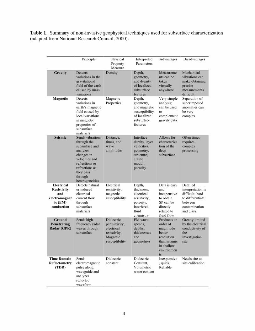
Table 1. Summary of non-invasive geophysical techniques used for subsurface characterization (adapted from National Research Council, 2000).

Principle Physical Property Measure

Interpreted Parameters

Advantages Disadvantages

Gravity Detects variations in the gravitational field of the earth caused by mass variations

Density Depth, geometry, and density of localized subsurface features

Measurements can be taken virtually anywhere

Mechanical vibrations can make obtaining precise measurements difficult

Magnetic Detects variations in earth’s magnetic field caused by local variations in magnetic properties of subsurface materials

Magnetic Properties

Depth, geometry, and magnetic susceptibility of localized subsurface features

Very simple analysis; can be used to complement gravity data

Separation of superimposed anomalies can be very complex

Seismic Sends vibrations through the subsurface and analyzes changes in velocities and reflections or refractions as they pass through heterogeneities

Distance, times, and wave amplitudes

Interface depths, layer velocities, geometry, structure, elastic moduli, porosity

Allows for characterization of the deep subsurface

Often times requires complex processing

Electrical Resistivity

and electromagnet

ic (EM) conduction

Detects natural or induced electrical current flow through subsurface materials

Electrical resistivity, magnetic susceptibility

Depth, thickness, electrical resistivity, porosity, interfered fluid chemistry

Data is easy and inexpensive to obtain, SP can be directly related to fluid flow

Detailed interpretation is difficult; hard to differentiate between contamination and clays

Ground Penetrating

Radar (GPR)

Sends high-frequency radar waves through subsurface

Dielectric permittivity, electrical resistivity, Magnetic susceptibility

EM wave speeds, depths, thicknesses and geometries

Produces an order of magnitude better resolution than seismic in shallow environments

Greatly limited by the electrical conductivity of the investigation site

Time Domain Reflectometry

(TDR)

Sends electromagnetic pulse along waveguide and analyzes reflected waveform

Dielectric constant

Dielectric Constant, Volumetric water content

Inexpensive, quick, Reliable

Needs site to site calibration

5

3. Locate land mines and unexploded ordnance

4. Identify underground instabilities that could lead to hazards such as earthquakes and

landslides

5. Identify buried objects or buried disturbed ground in archaeology studies

6. Identify geologic materials’ distribution and properties for basic science inquiry.

(National Research Council, 2000).

Some characterizations studies are less complex than others. For example, a comprehensive

geologic characterization must consider the inter-related lithology, stratigraphy, structure,

fractures, fluids, heterogeneities and fluid composition. In other scenarios the characterization

may only require resolving a buried object from its surrounding materials.

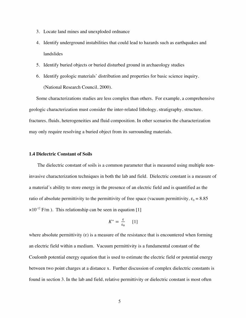
1.4 Dielectric Constant of Soils

The dielectric constant of soils is a common parameter that is measured using multiple non-

invasive characterization techniques in both the lab and field. Dielectric constant is a measure of

a material’s ability to store energy in the presence of an electric field and is quantified as the

ratio of absolute permittivity to the permittivity of free space (vacuum permittivity, ε0 = 8.85

×10-12 F/m ). This relationship can be seen in equation [1]

!∗ =   !!!

[1]

where absolute permittivity (ε) is a measure of the resistance that is encountered when forming

an electric field within a medium. Vacuum permittivity is a fundamental constant of the

Coulomb potential energy equation that is used to estimate the electric field or potential energy

between two point charges at a distance x. Further discussion of complex dielectric constants is

found in section 3. In the lab and field, relative permittivity or dielectric constant is most often

6

measured by placing a material between the two plates of a capacitor and measuring the ratio of

capacitance of the material to free space. It can also be measured by packing material around a

coaxial transmission line and measuring the resulting impedance or impedance changes due to

the application of an electric field (Fellner-Feldegg 1969). GPR is another technique that can be

used in the field and estimates the dielectric constant of subsurface environments as a function of

electromagnetic wave speed. The goal of this study was to increase the understanding of

dielectric behavior in porous materials through the use of Time Domain reflectometry, a non-

invasive geophysical technique that is believed to “hold promise for rapid, low-impact and

relatively inexpensive characterization of the heterogeneous subsurface” (National Research

Council, 2000).

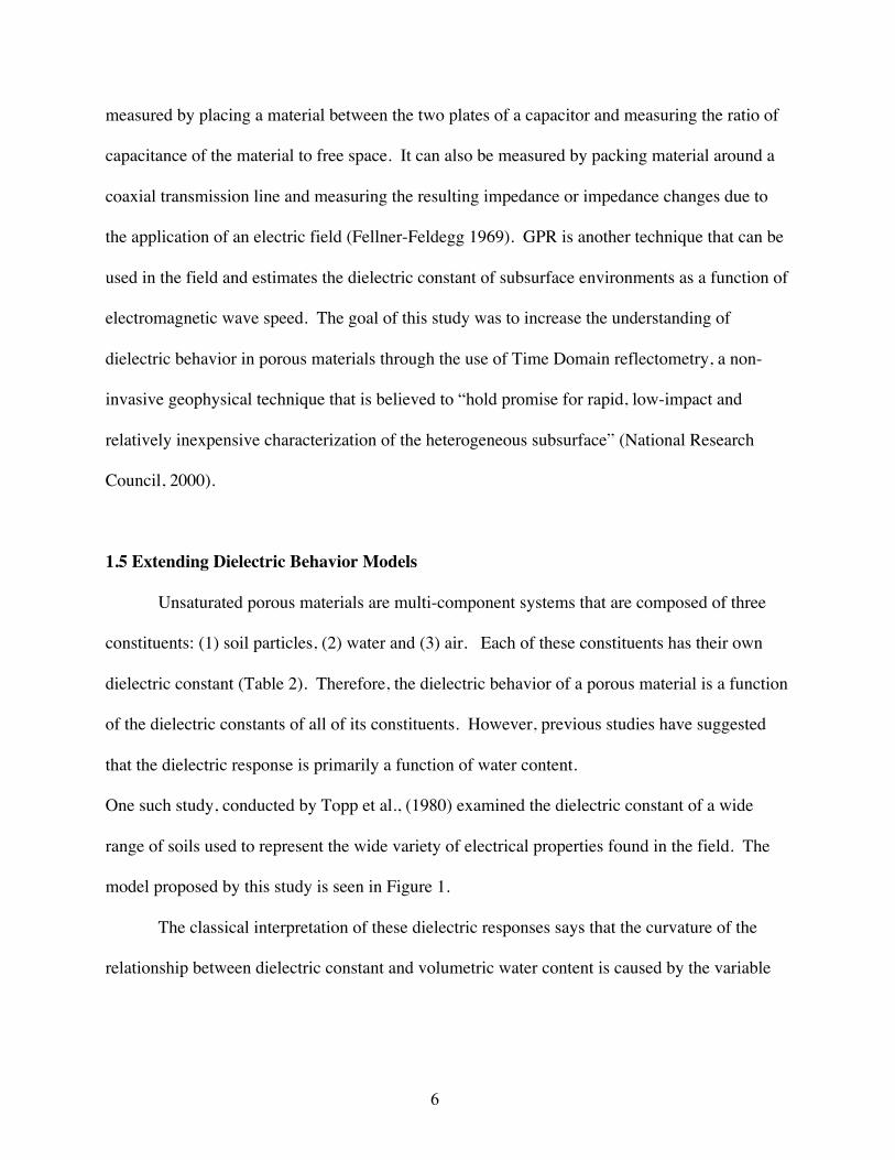
1.5 Extending Dielectric Behavior Models

Unsaturated porous materials are multi-component systems that are composed of three

constituents: (1) soil particles, (2) water and (3) air. Each of these constituents has their own

dielectric constant (Table 2). Therefore, the dielectric behavior of a porous material is a function

of the dielectric constants of all of its constituents. However, previous studies have suggested

that the dielectric response is primarily a function of water content.

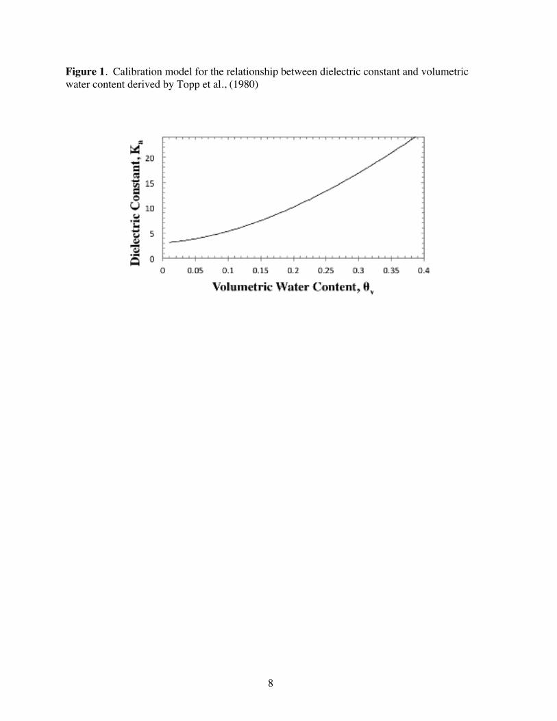
One such study, conducted by Topp et al., (1980) examined the dielectric constant of a wide

range of soils used to represent the wide variety of electrical properties found in the field. The

model proposed by this study is seen in Figure 1.

The classical interpretation of these dielectric responses says that the curvature of the

relationship between dielectric constant and volumetric water content is caused by the variable

7

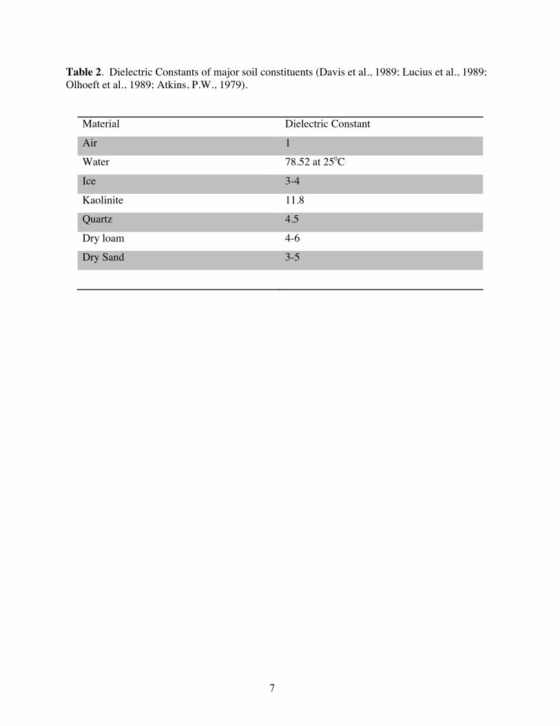
Table 2. Dielectric Constants of major soil constituents (Davis et al., 1989; Lucius et al., 1989; Olhoeft et al., 1989; Atkins, P.W., 1979).

Material Dielectric Constant

Air 1

Water 78.52 at 250C

Ice 3-4

Kaolinite 11.8

Quartz 4.5

Dry loam 4-6

Dry Sand 3-5

8

Figure 1. Calibration model for the relationship between dielectric constant and volumetric water content derived by Topp et al., (1980)

9

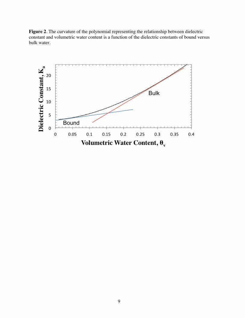
Figure 2. The curvature of the polynomial representing the relationship between dielectric constant and volumetric water content is a function of the dielectric constants of bound versus bulk water.

Bound

Bulk

10

contributions of bound versus bulk water (Hallaikainen et al., 1985; Topp et al., 1980; Wang et

al., 1986) (Figure 2). Figure 3 illustrates bound versus bulk water where bound water is defined

as the first three molecular layers of water along grain boundaries that exhibit a dielectric

constant similar to that of water contained in various ice structures, approximately 3 (Knight,

per. comm., 2012; Topp et al., 1980). Bulk fluid is not limited by interactions with the grain

surface and as a result has the high dielectric constant typically characteristic of water,

approximately 80 (Topp et al., 1980). The classical interpretation stated above suggests that

current models could be extended by accounting for different types of mineral constituents that

affect the ratio and properties of bound water. Therefore the hypothesis of this study was that the

dielectric responses of porous materials are mineral specific through differences in surface area

and chemistry.

A Control experiment was first developed with pure quartz sand and deionized water.

The Control established a baseline for the pure quartz-water system. Quartz sand/kaolin clay

mixtures were then used to vary the total surface area and mineralogy using clay that cannot

acquire interlayer water. Finally, iron oxyhydroxide coated quartz sand was used to change the

surface chemistry and charge on the quartz grain surfaces.

11

Figure 3. Quantitative illustration of bound versus bulk water in the pore space of porous materials. Wilting point is defined as the water content at which the soil tension is approximately 15 bars and it becomes difficult for plants to remove water. Field capacity is defined as the water content at which the soil tension is about 1/3 bars and water is able to flow with gravity.

Bound Bulk

Wilting  Point Field  Capacity

15  bars 1/3  barMineral  Grain

12

2. Background: Modeling the Dielectric Behavior of Unsaturated Soils

2.1 Traditional Dielectric Behavior Models for Soils

The previous discussion demonstrated that soils represent multi-component systems

consisting of mineral particles, air, free, and bound water. There is a consensus in the literature

that the dielectric response of a soil is a function of all four of these components (Halliainen, eta

l., 1985; Ledieu et al., 1986; Topp et al., 1989). The distribution of free and bound water is

directly proportional to the specific surface area of the material, which is controlled by texture.

The dielectric constant of these two components is dependent on frequency, temperature and

salinity. Therefore, the dielectric response of a soil is a function of (Hallikainen, Ulaby et al.

1985):

1. Frequency

2. Temperature

3. Salinity

4. Total water volume

5. Distribution of free and bound water (controlled by texture)

6. Mineral particles

7. Air

Although all of these factors are recognized, there are inconsistencies in the literature regarding

the degree to which each of these parameters influences the dielectric response and the

importance of including them into dielectric behavior models. This chapter discusses a number

of the more widely accepted models that have been proposed for estimating the effective

dielectric constant of multi-component systems. The differences between these models often

relates to their intended application. Two of the common applications with very different goals

13

include models used to estimate volumetric water content in the field and models used to

quantitatively better understand the dielectric behavior of soils. Although differences between

models often relates to application, fundamental differences exist in the understanding of

dielectric behavior in porous materials.

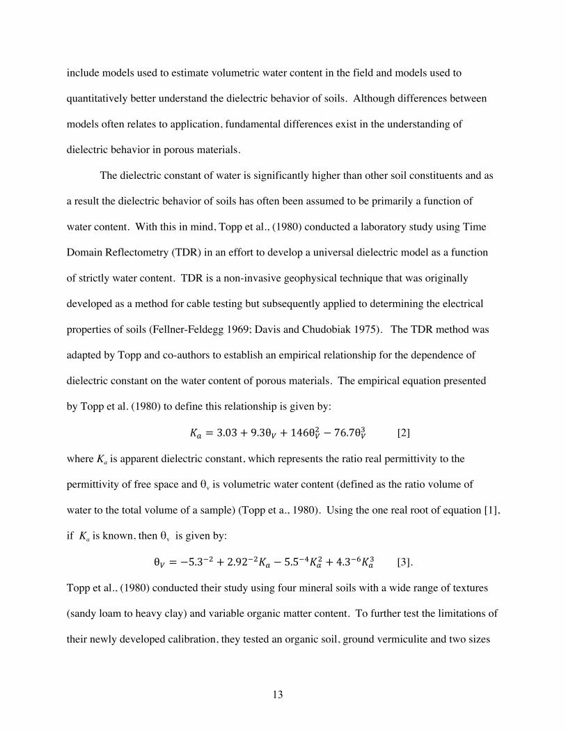
The dielectric constant of water is significantly higher than other soil constituents and as

a result the dielectric behavior of soils has often been assumed to be primarily a function of

water content. With this in mind, Topp et al., (1980) conducted a laboratory study using Time

Domain Reflectometry (TDR) in an effort to develop a universal dielectric model as a function

of strictly water content. TDR is a non-invasive geophysical technique that was originally

developed as a method for cable testing but subsequently applied to determining the electrical

properties of soils (Fellner-Feldegg 1969; Davis and Chudobiak 1975). The TDR method was

adapted by Topp and co-authors to establish an empirical relationship for the dependence of

dielectric constant on the water content of porous materials. The empirical equation presented

by Topp et al. (1980) to define this relationship is given by:

!! = 3.03+ 9.3θ! + 146θ!! − 76.7θ!! [2]

where Ka is apparent dielectric constant, which represents the ratio real permittivity to the

permittivity of free space and θv is volumetric water content (defined as the ratio volume of

water to the total volume of a sample) (Topp et a., 1980). Using the one real root of equation [1],

if Ka is known, then θv is given by:

θ! = −5.3!! + 2.92!!!! − 5.5!!!!! + 4.3!!!!! [3].

Topp et al., (1980) conducted their study using four mineral soils with a wide range of textures

(sandy loam to heavy clay) and variable organic matter content. To further test the limitations of

their newly developed calibration, they tested an organic soil, ground vermiculite and two sizes

14

of glass beads. It was assumed that these materials represented the wide variety of electrical

properties found in common soils (Topp et al., 1980). In their study, Topp et al. (1980)

concluded there is an empirical relationship between dielectric constant and water content (Eq. 2)

and that for the frequency range of 1 MHz to 1 GHz this relationship is independent of

frequency, soil type, soil density, soil temperature and soluble salt content. In the study, any

variation in soil type was reported to lead to an error of less than 1.3%.

Six years later, Ledieu et al., (1986) conducted a similar experiment using field samples

within the lab to model dielectric responses using water contents. The compositions of the field

samples used by Ledieu and others were not sufficiently described in the paper. Samples were

referred to as “loams” without any characterization of whether the loams referred to clay loams,

sand loams or a range of both. The term “loam” is a quantitative description of soil texture that

refers to variable proportions of clay, silt and sand. The relationship proposed by Ledieu et al.,

(1986) is seen in equation [4].

!! =  !!!!.!"#$!.!!"#

! [4]

If Ka is known, θv is given by:

θ! = 0.1138 !! − 0.1758 [5]

Similar to Topp et al., (1980), Ledieu et al., (1986) concluded that dielectric constant values were

almost entirely a function of water content alone. According to Ledieu and others, any effects

arising from the nature of the soil and its constituents on the dominant relationship between

dielectric constant and volumetric water content are negligible. The study showed that variations

in soil type produced an error of less than 1%.

15

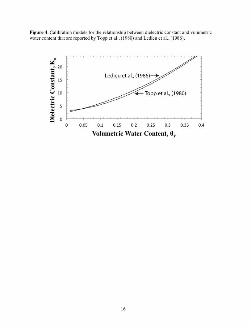
This calibration, as well as the one presented by Topp et al., (1986) is shown in Figure 4.

Although these two experiments had very different setups and the samples used by Ledieu et al.,

(1986) are poorly characterized, the results show that the two plots fall within the

16

Topp et al., (1980)

Ledieu et al., (1986)

Figure 4. Calibration models for the relationship between dielectric constant and volumetric water content that are reported by Topp et al., (1980) and Ledieu et al., (1986).

17

error ranges in water content reported for each study. For this reason, these two calibrations are

often cited and provide what many believe to be sufficient evidence that the dielectric constant of

a soil is almost entirely a simple function of water content.

Despite their conclusions, Topp et al., (1980) noticed that texture affected the shape of

their polynomial through the influence of surface area, suggesting that additional factors may

play a role in the dielectric response of soils. Other studies (Wang et al., 1980; Hallikainen,

Ulaby et al. 1985) suggest this is indeed true and show inconsistencies between the dielectric

constants of different soil types at the same water contents.

Recognizing the potential for these additional influences to affect the dielectric response

of a soil, some studies avoid the Topp et al. (1980) and Ledieu et al. (1986) models. Instead,

they use field site-specific models that inherently account for the texture of the local soil

(Jacobsen 1993; Chandler 2004). There are two ways to develop these site-specific models. First,

soils can be collected from the site of interest and returned to the lab to develop a new empirical

relationship between dielectric constant and volumetric water content in a way that is similar to

the techniques used by Topp et al. (1980) and Ledieu et al. (1986). The advantage of this

technique is that the new model is site-specific, making it particularly advantageous for use in

areas with soils that are laterally and vertically homogeneous. There are also disadvantages.

First, large heterogeneities within the site will create problems similar to the application of the

Topp et al. (1980) and Ledieu et al. (1986) models. Second, this site-specific technique is time

consuming and expensive because the cost of developing a new calibration increases rapidly

when deeper soils need to be investigated. Most importantly, this technique still does not

quantitatively assess the effects of specific soil parameters on the dielectric response of a soil.

18

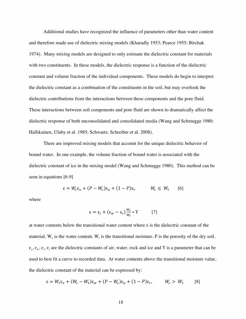
Additional studies have recognized the influence of parameters other than water content

and therefore made use of dielectric mixing models (Kharadly 1953; Pearce 1955; Birchak

1974). Many mixing models are designed to only estimate the dielectric constant for materials

with two constituents. In these models, the dielectric response is a function of the dielectric

constant and volume fraction of the individual components. These models do begin to interpret

the dielectric constant as a combination of the constituents in the soil, but may overlook the

dielectric contributions from the interactions between these components and the pore fluid.

These interactions between soil components and pore fluid are shown to dramatically affect the

dielectric response of both unconsolidated and consolidated media (Wang and Schmugge 1980;

Hallikainen, Ulaby et al. 1985; Schwartz, Schreiber et al. 2008).

There are improved mixing models that account for the unique dielectric behavior of

bound water. In one example, the volume fraction of bound water is associated with the

dielectric constant of ice in the mixing model (Wang and Schmugge 1980). This method can be

seen in equations [6-9]

ε =!!ε! + ! −!! ε! + 1− ! ε!                            !! ≤  !! [6]

where

ε = ε! + ε! − ε!!!!!∗ Υ [7]

at water contents below the transitional water content where ε is the dielectric constant of the

material, Wc is the water content, Wt is the transitional moisture, P is the porosity of the dry soil,

εa, εw, εr, εi are the dielectric constants of air, water, rock and ice and Υ is a parameter that can be

used to best fit a curve to recorded data. At water contents above the transitional moisture value,

the dielectric constant of the material can be expressed by:

ε =!!ε! + !! −!! ε! + ! −!! ε! + 1− ! ε! ,                        !! >  !! [8]

19

where

ε! = ε! + ε! − ε! ∗ Υ [9]

The disadvantage of this type of technique is that it can also be extremely difficult to implement

in areas that are highly complex and heterogeneous.

Many of the models derived to estimate the dielectric constant of multi-component

systems and specifically the ones associated with TDR (Topp et al., (1980) and Ledieu et al.,

(1986)) do not account for the dielectric contributions of soil constituents other than water.

These overlooked constituents that contribute to the behavior of these multi-component systems

have been shown to have a large impact on the dielectric response of a soil. It is believed that

the dielectric contribution of these other components is related to their interactions with pore

fluid at the solid-fluid interface (Wang and Schmugge 1980; Hallikainen, Ulaby et al. 1985;

Schwartz, Schreiber et al. 2008). Clearly, there is a need for dielectric behavior models that have

the ability to account for the significant dielectric contributions of these interactions. Clay

contents and mineral coatings are two soil parameters investigated in this study which I believe

to have unique interactions with pore fluid and therefore have the potential to contribute to the

overall dielectric response of a soil.

20

3. Background: Dielectrics and Porous Media

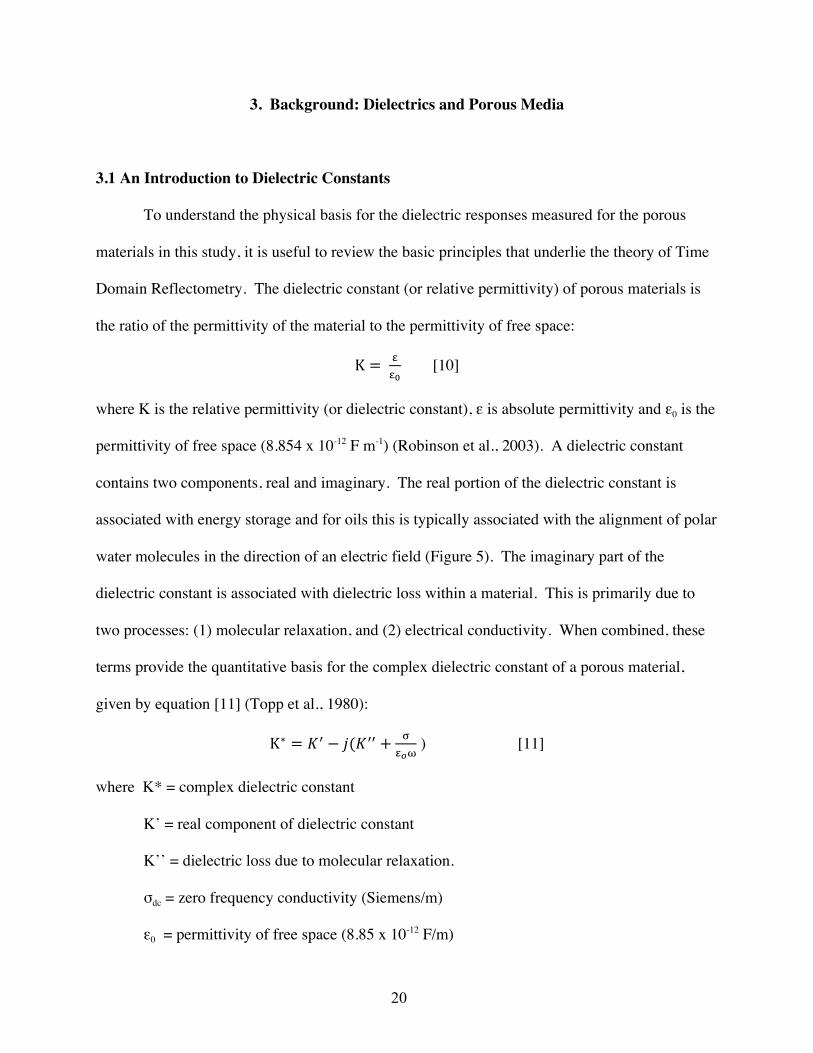
3.1 An Introduction to Dielectric Constants

To understand the physical basis for the dielectric responses measured for the porous

materials in this study, it is useful to review the basic principles that underlie the theory of Time

Domain Reflectometry. The dielectric constant (or relative permittivity) of porous materials is

the ratio of the permittivity of the material to the permittivity of free space:

K =   !!!

[10]

where K is the relative permittivity (or dielectric constant), ε is absolute permittivity and ε0 is the

permittivity of free space (8.854 x 10-12 F m-1) (Robinson et al., 2003). A dielectric constant

contains two components, real and imaginary. The real portion of the dielectric constant is

associated with energy storage and for oils this is typically associated with the alignment of polar

water molecules in the direction of an electric field (Figure 5). The imaginary part of the

dielectric constant is associated with dielectric loss within a material. This is primarily due to

two processes: (1) molecular relaxation, and (2) electrical conductivity. When combined, these

terms provide the quantitative basis for the complex dielectric constant of a porous material,

given by equation [11] (Topp et al., 1980):

K∗ = !! − !(!!! + !!!!

) [11]

where K* = complex dielectric constant

K’ = real component of dielectric constant

K’’ = dielectric loss due to molecular relaxation.

σdc = zero frequency conductivity (Siemens/m)

ε0 = permittivity of free space (8.85 x 10-12 F/m)

21

Figure 5. Water molecules with no orientation (left) due to thermal motion and (right) the organization of water molecules in the presence of an electric field. Figure after Robinson et al., (2003).

Thermal motion causes random

orientation of water molecules

Organization of water

molecules in the presence

of an electric field

22

ω = angular frequency (radians/sec)

j = (-1)^1/2

At high frequencies of 100 MHz-4 GHz, K’ is independent of frequency (Ledieu et al., 1986).

Therefore, there are no relaxation mechanisms that would lead to dielectric loss as heat. It has

also been shown that in this frequency range, the dielectric loss due to electrical conduction is

negligible (Ledieu et al., 1986). Therefore at high frequencies, such as those used in TDR

measurements, the dielectric constant of a material is almost entirely real. Although the effect of

electrical loss exists in measurements, it is not measureable and therefore it can be assumed that

K’≈ Ka, where Ka is known as the apparent dielectric constant.

3.2 Estimating Dielectric Constant Using TDR

TDR systems are designed to obtain the apparent dielectric constant of a porous media by taking

advantage of two relationships. First, the travel time for an electromagnetic signal through earth

materials with relatively low conductivity and relative magnetic permeability is dependent on

both the velocity of a signal as well as the length of a waveguide, as given by equation [12]

∆! =   !!!

[12]

where Δt is the travel time, L is the length of the waveguide, and v is the velocity of

electromagnetic signals in the sample media (Robinson et al., 2003). Second, the velocity of the

signal is dependent upon the apparent dielectric constant of the material that surrounds the

waveguide:

! =   !!!

[13]

where V is the velocity of light in the sample media, c is the velocity of light in free space

(3x108) (ms-1), and Ka is the apparent dielectric constant of the material surrounding the

23

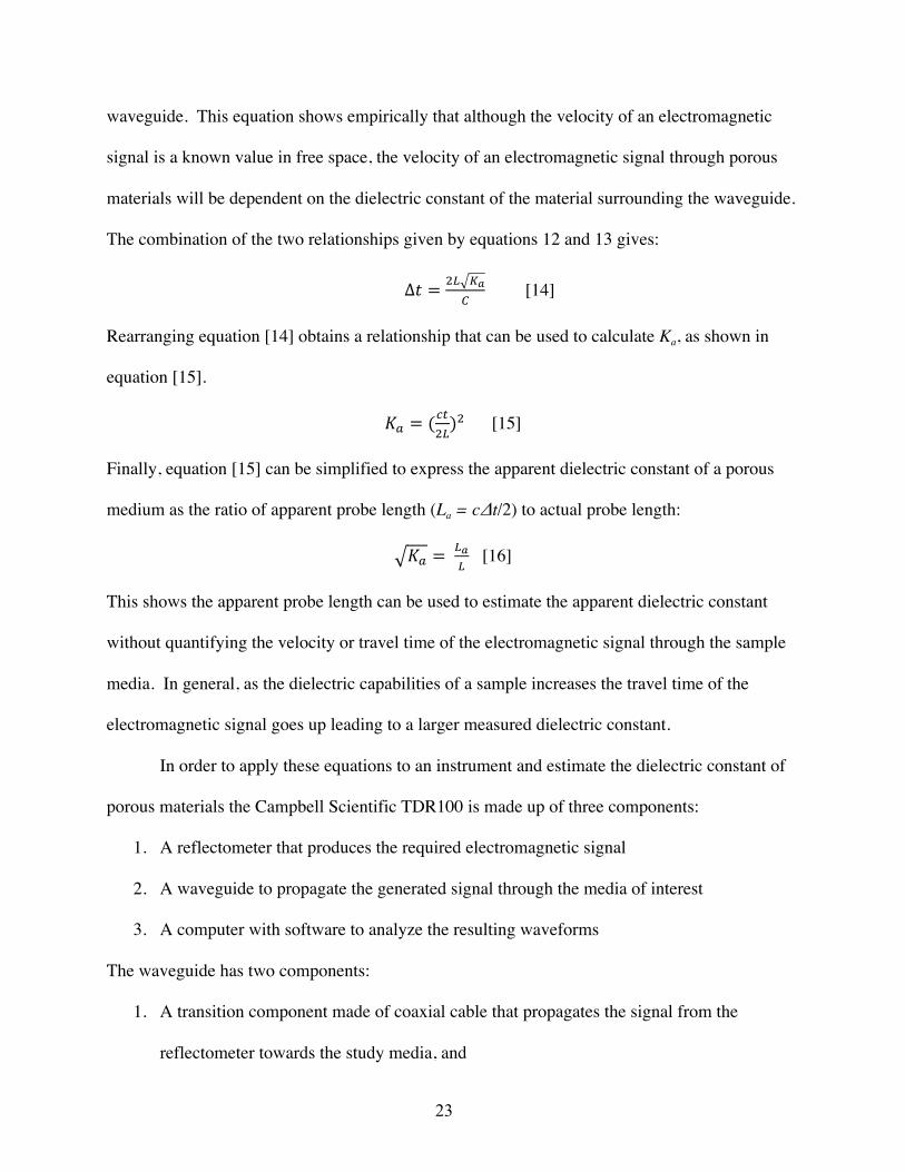
waveguide. This equation shows empirically that although the velocity of an electromagnetic

signal is a known value in free space, the velocity of an electromagnetic signal through porous

materials will be dependent on the dielectric constant of the material surrounding the waveguide.

The combination of the two relationships given by equations 12 and 13 gives:

∆! = !! !!!

[14]

Rearranging equation [14] obtains a relationship that can be used to calculate Ka, as shown in

equation [15].

!! = (!"!!)! [15]

Finally, equation [15] can be simplified to express the apparent dielectric constant of a porous

medium as the ratio of apparent probe length (La = cΔt/2) to actual probe length:

!! =  !!!

[16]

This shows the apparent probe length can be used to estimate the apparent dielectric constant

without quantifying the velocity or travel time of the electromagnetic signal through the sample

media. In general, as the dielectric capabilities of a sample increases the travel time of the

electromagnetic signal goes up leading to a larger measured dielectric constant.

In order to apply these equations to an instrument and estimate the dielectric constant of

porous materials the Campbell Scientific TDR100 is made up of three components:

1. A reflectometer that produces the required electromagnetic signal

2. A waveguide to propagate the generated signal through the media of interest

3. A computer with software to analyze the resulting waveforms

The waveguide has two components:

1. A transition component made of coaxial cable that propagates the signal from the

reflectometer towards the study media, and

24

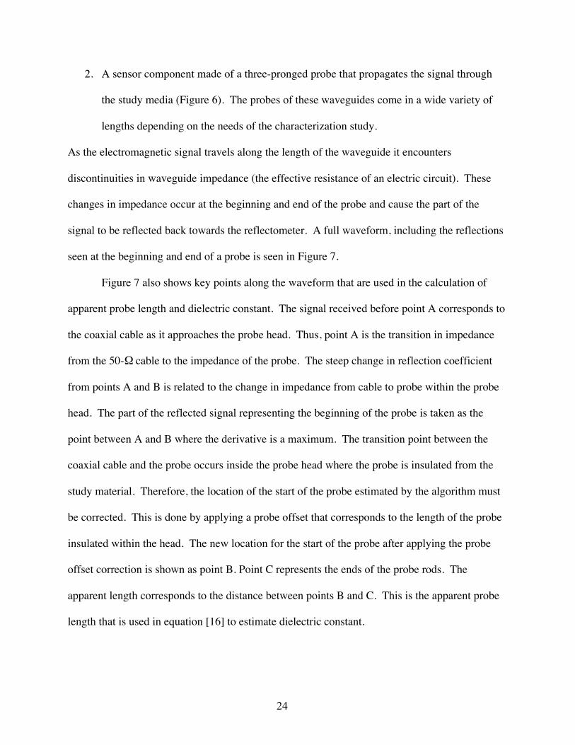
2. A sensor component made of a three-pronged probe that propagates the signal through

the study media (Figure 6). The probes of these waveguides come in a wide variety of

lengths depending on the needs of the characterization study.

As the electromagnetic signal travels along the length of the waveguide it encounters

discontinuities in waveguide impedance (the effective resistance of an electric circuit). These

changes in impedance occur at the beginning and end of the probe and cause the part of the

signal to be reflected back towards the reflectometer. A full waveform, including the reflections

seen at the beginning and end of a probe is seen in Figure 7.

Figure 7 also shows key points along the waveform that are used in the calculation of

apparent probe length and dielectric constant. The signal received before point A corresponds to

the coaxial cable as it approaches the probe head. Thus, point A is the transition in impedance

from the 50-Ω cable to the impedance of the probe. The steep change in reflection coefficient

from points A and B is related to the change in impedance from cable to probe within the probe

head. The part of the reflected signal representing the beginning of the probe is taken as the

point between A and B where the derivative is a maximum. The transition point between the

coaxial cable and the probe occurs inside the probe head where the probe is insulated from the

study material. Therefore, the location of the start of the probe estimated by the algorithm must

be corrected. This is done by applying a probe offset that corresponds to the length of the probe

insulated within the head. The new location for the start of the probe after applying the probe

offset correction is shown as point B. Point C represents the ends of the probe rods. The

apparent length corresponds to the distance between points B and C. This is the apparent probe

length that is used in equation [16] to estimate dielectric constant.

25

Figure 6. Illustration of the probe component of the TDR100 waveguide that is inserted into the study media for electromagnetic wave propagation. Figure is not to scale.

Coaxial Cable

Vp = 0.67

Resistance = 50 ohms

Probe Head

Length = 5.75 cm

Width = 4.0 cm

Thickness = 1.25 cm

Proble Prongs

Lenth = 15.0 cm

Diameter = 0.318 cm

15.0 cm

5.75 cm 4.0  cm

152.4 cm

26

Figure 7. Schematic of a typical waveform recorded analyzed by the TDR100 with three key points labeled A, B and C (figure adapted from TDR100 instructional manual, Campbell Scientific). The waveform before point A represents the coaxial cable before the probe head. Point A represents the transition from the coaxial cable to the probe. The rapid change in reflection coefficient after point A is due to the change in impedance from the coaxial cable to the probe. Point B represents the point where the probe is no longer insulated by the probe head and makes contact with the study media. Point C represents the end of the probe. Apparent Length (La), the parameter calculated from the waveform and used to calculate the apparent dielectric constant, is the distance between points B and C.

A

B

C

0.1

0

-0.1

-0.2

-0.3

re!e

ctio

n co

e"ci

ent (

rho)

Distance (meters)

La

2 3 4 5

27

4. Materials and Methods

4.1 Introduction

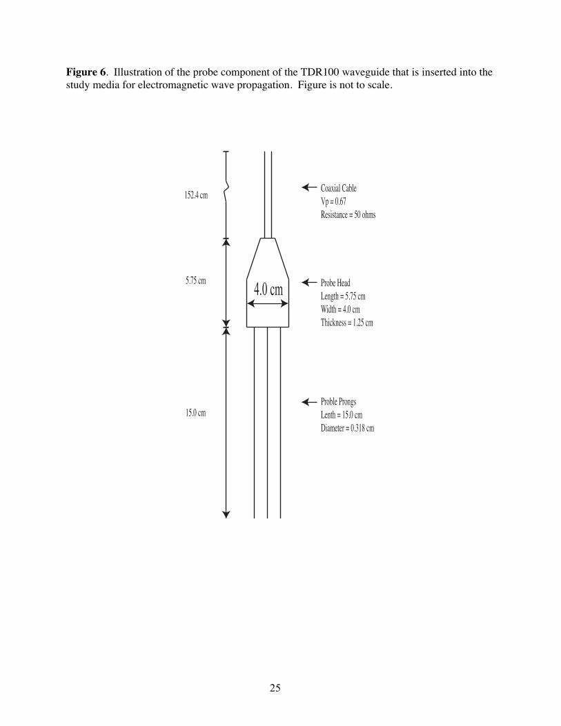
The experimental setup is shown in Figure 8. To conduct the experiments the sample

apparatus was filled with one of three types of media:

1. Pure quartz sand (Control)

2. Iron oxyhydroxide coated quartz sand

3. Quartz sand/ kaolin clay mixtures with clay contents that vary from zero (Control) to

eight weight percent

The sample apparatus was connected to the Campbell Scientific TDR100 system that was used to

estimate the dielectric constant, an air bubbler to maintain the humidity within the sample

apparatus and a vacuum pump to accelerate the draining of the initially saturated sample. To

make measurements, the pumping was stopped to collect a dielectric constant value from the

TDR100 and a volumetric water content value. To obtain the water content, the sample

apparatus was placed on a scale to measure the difference in “wet” and “dry” weights. This

method produced data that showed:

1. The relationship between dielectric constant, volumetric water content, and weight

percent clay content

2. The effect of iron oxyhydroxide on the relationship between dielectric constant and

volumetric content.

28

Figure 8. Illustration of the experimental design. The TDR probe is connected to the TDR100, power source and computer running PCTDR software. The sample apparatus is connected to the solution trap flask and vacuum pump as well as an air bubbler to control humidity.

BatteryCampbell Scienti!cTDR100

Computer with PCTDR Software

Vacuum Pump

Solution Trap Flask

Sample Appartatus

Air Intake

Air Bubbler

Deionized Water TDR probe

29

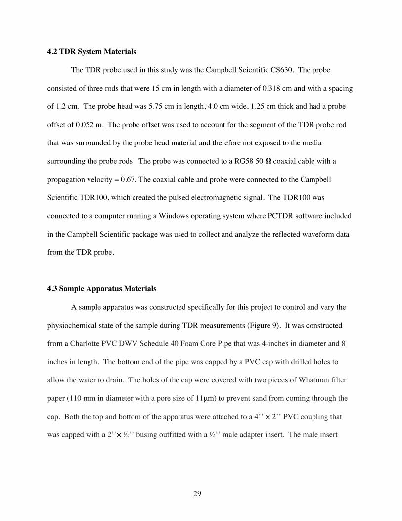
4.2 TDR System Materials

The TDR probe used in this study was the Campbell Scientific CS630. The probe

consisted of three rods that were 15 cm in length with a diameter of 0.318 cm and with a spacing

of 1.2 cm. The probe head was 5.75 cm in length, 4.0 cm wide, 1.25 cm thick and had a probe

offset of 0.052 m. The probe offset was used to account for the segment of the TDR probe rod

that was surrounded by the probe head material and therefore not exposed to the media

surrounding the probe rods. The probe was connected to a RG58 50 Ω coaxial cable with a

propagation velocity = 0.67. The coaxial cable and probe were connected to the Campbell

Scientific TDR100, which created the pulsed electromagnetic signal. The TDR100 was

connected to a computer running a Windows operating system where PCTDR software included

in the Campbell Scientific package was used to collect and analyze the reflected waveform data

from the TDR probe.

4.3 Sample Apparatus Materials

A sample apparatus was constructed specifically for this project to control and vary the

physiochemical state of the sample during TDR measurements (Figure 9). It was constructed

from a Charlotte PVC DWV Schedule 40 Foam Core Pipe that was 4-inches in diameter and 8

inches in length. The bottom end of the pipe was capped by a PVC cap with drilled holes to

allow the water to drain. The holes of the cap were covered with two pieces of Whatman filter

paper (110 mm in diameter with a pore size of 11μm) to prevent sand from coming through the

cap. Both the top and bottom of the apparatus were attached to a 4’’ × 2’’ PVC coupling that

was capped with a 2’’× ½’’ busing outfitted with a ½’’ male adapter insert. The male insert

30

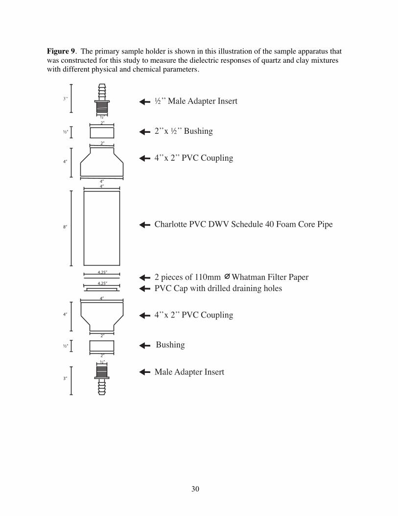
Figure 9. The primary sample holder is shown in this illustration of the sample apparatus that was constructed for this study to measure the dielectric responses of quartz and clay mixtures with different physical and chemical parameters.

Charlotte PVC DWV Schedule 40 Foam Core Pipe

2 pieces of 110mm Whatman Filter Paper

PVC Cap with drilled draining holes

4’’x 2’’ PVC Coupling

Bushing

Male Adapter Insert

2’’x ½’’ Bushing

½’’ Male Adapter Insert

4’’x 2’’ PVC Coupling

8’’

4’’4’’

2’’

2’’

4.25’’

4.25’’

4’’

2’’

2’’!’’

!’’

!’’

!’’

4’’

4’’

3’’

3’’

31

projecting from the top of the sample apparatus connected to vinyl tubing that led to the air

bubbler used to control the humidity within the sample apparatus. The air bubbler created 100%

humidity within the sample apparatus. This insured the water loss from the media was the result

of physical separation between the grains and the pore water by draining rather than by

evaporation, which would lead to a heterogeneous water distribution. The male insert coming

from the bottom of the sample apparatus connected to vinyl tubing that to led to the vacuum

pump, which was used to accelerate draining of the various samples.

4.4 Experimental Procedure for the Control and kaolin Clay/Quartz Sand Mixtures

All of the quartz material used in the experiments consisted of pure ASTM 20-30 Ottawa

silica sand (median grain diameter of 0.6 mm, 90% passes #20 sieve, 95% retained on #30

sieve). Pure quartz sand was first saturated with deionized water and served as the Control for

the clay and iron treatments. This mineral/fluid composition was used to develop a baseline for

the relationship between dielectric constant and volumetric water content. Controlled amounts

of kaolin clay, purchased from Minnesota Clay (2960 Niagara Lane, Plymouth, Minnesota), was

added to the quartz sand in order to test the textural effects of porous media on dielectric

constants. Table 3 summarizes the properties of kaolin clay (Dove, In preparation). The

experiment was run using 0, 2, 4, 6 and 8 weight percent clay contents. The pumping times for

the different clay treated samples were expected to increase dramatically and observations of this

behavior are described in the results and discussion section. The experimental procedure for the

kaolin clay mixtures was as follows:

1. Wash any unused ASTM 20-30 Ottawa Silica Sand in a deionized water bath five (5) times to remove small particulates

2. Oven dry the quartz sand overnight

32

Table 3. Summary of the geochemical index properties for the Kaolin clay used in the quartz sand/kaolin clay mixtures. Activity (A) = PI (%) divided by the % clay fraction, where PI is the plasticity index from an Atterberg limits test. % Clay fraction is the percentage of the whole sample that is smaller than 2 microns (Dove, pers. comm., 2012).

Soil pH (In water)

CEC (cmol(+)/kg)

BET Specific Surface Area

(m2/g)

Activity

Kaolin Clay 6.46 2.1 22.45 0.77

33

3. Weigh the sample apparatus including the top and bottom couplings as well as the TDR probe. This weight, added to the weight of the sample media, was the dry weight that was used to calculate volumetric water content

4. Remove the top coupling and probe and suspend the apparatus on a ring stand. Make sure that the apparatus is attached to the bottom coupling and bushing that leads to the vacuum pump.

5. Measure 550 grams of combined dry sand and clay, varying the proportions of each to achieve the desired weight percent clay for each trial.

6. Mix the clay and sand together using a small amount of water. The clay should stick to the sand grains without aggregating.

7. Add the mixture to the sample apparatus and saturate to achieve regular grain packing 8. Repeat steps 5-7 three times to obtain four lifts and a sample that has a total weight of

2.2 kg and fills the sample apparatus. 9. Ensure that the sample is fully saturated 10. Insert the probe into the saturated media while attaching the top coupling that leads to

the air bubbler. 11. Secure both the top and bottom couplings to the PVC pipe with electrical tape to

ensure no air leaks. 12. Begin pumping. 13. Halt pumping when a small amount of water comes out of the apparatus. Pumping

times were very short at first and then increased exponentially as volumetric water content decreased. Pumping times also increased significantly with increased clay content.

14. Remove top and bottom bushings and place sample apparatus on a scale to get a wet weight measurement.

15. While sample apparatus is on the scale, use PCTDR to estimate the dielectric constant.

16. Place sample apparatus back on the ring stand and re-attach top and bottom bushings. 17. Repeat steps 11-15 until the weight of the apparatus is constant with continued

pumping. 18. Plot the dielectric constant vs. water content to evaluate the effect of the treatment.

By comparing the baseline curve (measured for the Control) with the relationships found

in clay treated samples, the experiments were able to evaluate the effect of low clay contents on

the relationship between dielectric constant and volumetric water content.

4.5 Experimental Procedure for Iron Oxyhydroxide Coated Quartz Grains

The method used to prepare the quartz sand samples with ferric oxyhydroxide mineral

coatings was modified after the procedure described in Grantham and Dove, (1997) (Grantham,

34

1997). The quantity of materials was scaled up due to the larger amount of coated quartz sand

required for these experiments. Coatings were prepared using FeSO4 oxidation and precipitation

processes. The procedure began by mixing 40 drops of 30% H2O2 in 1000 ml of a 0.1 M FeSO4

solution. The solution was poured into a container containing the clean quartz surfaces, and left

overnight to allow the FeSO4 to oxidize. The resulting ferric-oxyhydroxide coated quartz grains

were removed from the solution, rinsed and dried overnight. The grains were then washed five

times in deionized water (15 minutes per cycle), dried over night at 100 degrees Celsius and used

for experiment. The experimental procedure for testing the iron oxyhydroxide coated quartz

samples was as follows:

1. Weigh the sample apparatus including the top and bottom couplings as well as the TDR probe. This weight, added to the weight of the sample media, was the dry weight that was used to calculate volumetric water content.

2. Remove the top coupling and probe and fill the sample apparatus with 2.2 kg of iron oxyhydroxide coated ASTM 20-30 Ottawa Silica Sand (median grain diameter of 0.6 mm, 90% passes #20 sieve, 95% is retained on #30 sieve) grains by raining from a constant height to obtain regular grain packing

3. Place the sample apparatus on the ring stand, attach the bottom bushing that leads to the vacuum pump and saturate the sample apparatus.

4. Insert the probe into the study media while attaching the top coupling and bushing that lead to the air bubbler.

5. Begin pumping 6. Stop pumping when a small amount of water comes out of the apparatus. Pumping times

were very short at first and then increased exponentially as volumetric water content decreased.

7. Remove top and bottom bushings and place sample apparatus on the center of the scale to get a wet weight measurement.

8. While sample apparatus is on the scale, use PCTDR to estimate the dielectric constant. 9. Place sample apparatus back on the ring stand and re-attach top and bottom bushings. 10. Repeat steps 11-15 until the weight of the apparatus is constant with continued pumping. 11. Plot dielectric constant vs. volumetric water content to evaluate the effect of the treatment

Using this experimental procedure, this study quantified how iron coatings along the surface

of the quartz grains affect the relationship dielectric constant versus volumetric water content.

35

5. Results and Discussion

5.1 Quartz Sand/kaolin Clay Observations Aggregation of the sample was a common occurrence during preparation when

attempting to bind the clay to the quartz sand with small amounts of water. It appears that fully

saturating the samples before each trial eliminated any difference in packing that might have led

to inconsistencies between trials. It was noticed that each sample subsided or settled with the

addition of water, which was observed to be consistent between trials. The effluent of the fully

saturated samples at the beginning of each trial was typically a cloudy white color indicating that

a small portion of the clay from the initial sample was being removed during the experiment. A

dry initial and final weight for the trap flask that captured solution removed from the apparatus

was recorded during each trial to quantify the amount of clay that was removed in solution.

These measurements showed that the changes in clay content due to clay being removed were

negligible.

At high water contents, the pumping times between data points for each trial were very

short, typically a few seconds. As water contents decreased the pumping times between data

points for each trial grew significantly. The pumping times also increased with increasing clay

content. In the control experiment, the collection of all the data points across the full range of

water contents typically lasted 24 hours. In comparison, the collection time for the 8 weight

percent clay sample required 120 hours (5 days). Once fully dry, all of the clay samples became

a consolidated media that was cemented by the clay between the quartz grains.

36

5.2 Quartz Sand Control Analysis

The raw data collected for this analysis is listed in Appendix A. A third degree

polynomial (Equation 17) describing the relationship between dielectric constant and volumetric

water content was first fit to the 0% clay Control data collected on two different days using the

least squares method (Figure 10).

!! = !! + !!θ+  !!!! +  !!θ! [17]

As mentioned previously, the Control experiments using quartz sand and deionized water

established the baseline for dielectric response in single mineral-water system. The high R2

value of 0.998 (Table 4) indicates that this model explains essentially all of the relationship

between dielectric constant and volumetric water content for the quartz-deionized water system.

A comparison between the Control polynomial and the model proposed by Topp et al. (1980)

shows good qualitative agreement between the two functions across all water contents (Figure

10). This led us to conclude that the Topp et al. (1980) model provides a good means of

estimating the dielectric constant of pure quartz-deionized water systems across water contents.

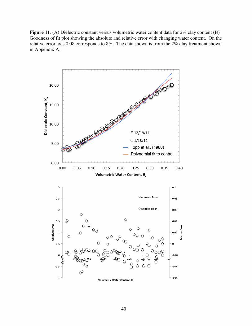
5.3 Quartz Sand/kaolin Clay Analysis

The raw data collected for this analysis is listed in Appendix A. A third degree

polynomial describing the relationship between dielectric constant and volumetric water content

was subsequently fit to the data for experiments conducted at each clay content, again using the

least squares method (Figures 11-14). These figures show the collected data points from two

different days, the polynomial fit to those data points as well as the Topp et al., (1980) model and

the polynomial fit to the Control data. The polynomials for each clay content data set are

summarized in Table 4. R2 values were >0.98 for each clay content, indicating that these models

37

explain essentially all of the relationship between Ka and θ at a given clay content. The

polynomials fit to the individual clay treatments show similar qualitative agreement to the Topp

et al., (1980) model as the polynomial fit to the Control data. Plotting all of the polynomials

from the individual clay treatments shows that the dielectric response of the quartz clay mixtures

do not suggest a changing contribution of bound versus bulk water (Figure 15).

38

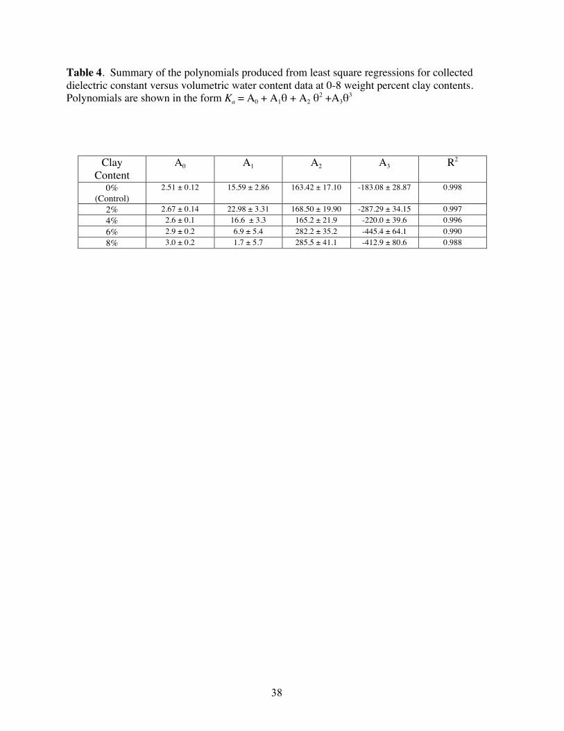
Table 4. Summary of the polynomials produced from least square regressions for collected dielectric constant versus volumetric water content data at 0-8 weight percent clay contents. Polynomials are shown in the form Ka = A0 + A1θ + A2 θ2 +A3θ3

Clay Content

A0 A1 A2 A3 R2

0% (Control)

2.51 ± 0.12 15.59 ± 2.86 163.42 ± 17.10 -183.08 ± 28.87 0.998

2% 2.67 ± 0.14 22.98 ± 3.31 168.50 ± 19.90 -287.29 ± 34.15 0.997 4% 2.6 ± 0.1 16.6 ± 3.3 165.2 ± 21.9 -220.0 ± 39.6 0.996 6% 2.9 ± 0.2 6.9 ± 5.4 282.2 ± 35.2 -445.4 ± 64.1 0.990 8% 3.0 ± 0.2 1.7 ± 5.7 285.5 ± 41.1 -412.9 ± 80.6 0.988

39

Figure 10. (A) Dielectric constant versus volumetric water content data for 0% clay content (Control) (B) Goodness of fit plot showing the absolute and relative error with changing water content. On the relative error axis 0.08 corresponds to 8%. The data shown is from the 0% clay treatment shown in Appendix A.

40

Figure 11. (A) Dielectric constant versus volumetric water content data for 2% clay content (B) Goodness of fit plot showing the absolute and relative error with changing water content. On the relative error axis 0.08 corresponds to 8%. The data shown is from the 2% clay treatment shown in Appendix A.

41

Figure 12. (A) Dielectric constant versus volumetric water content data for 4% clay content (B) Goodness of fit plot showing the absolute and relative error with changing water content. On the relative error axis 0.08 corresponds to 8%. The data shown is from the 4% clay treatment shown in Appendix A.

42

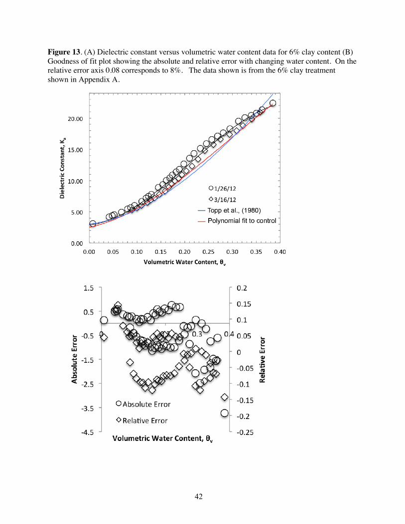
Figure 13. (A) Dielectric constant versus volumetric water content data for 6% clay content (B) Goodness of fit plot showing the absolute and relative error with changing water content. On the relative error axis 0.08 corresponds to 8%. The data shown is from the 6% clay treatment shown in Appendix A.

43

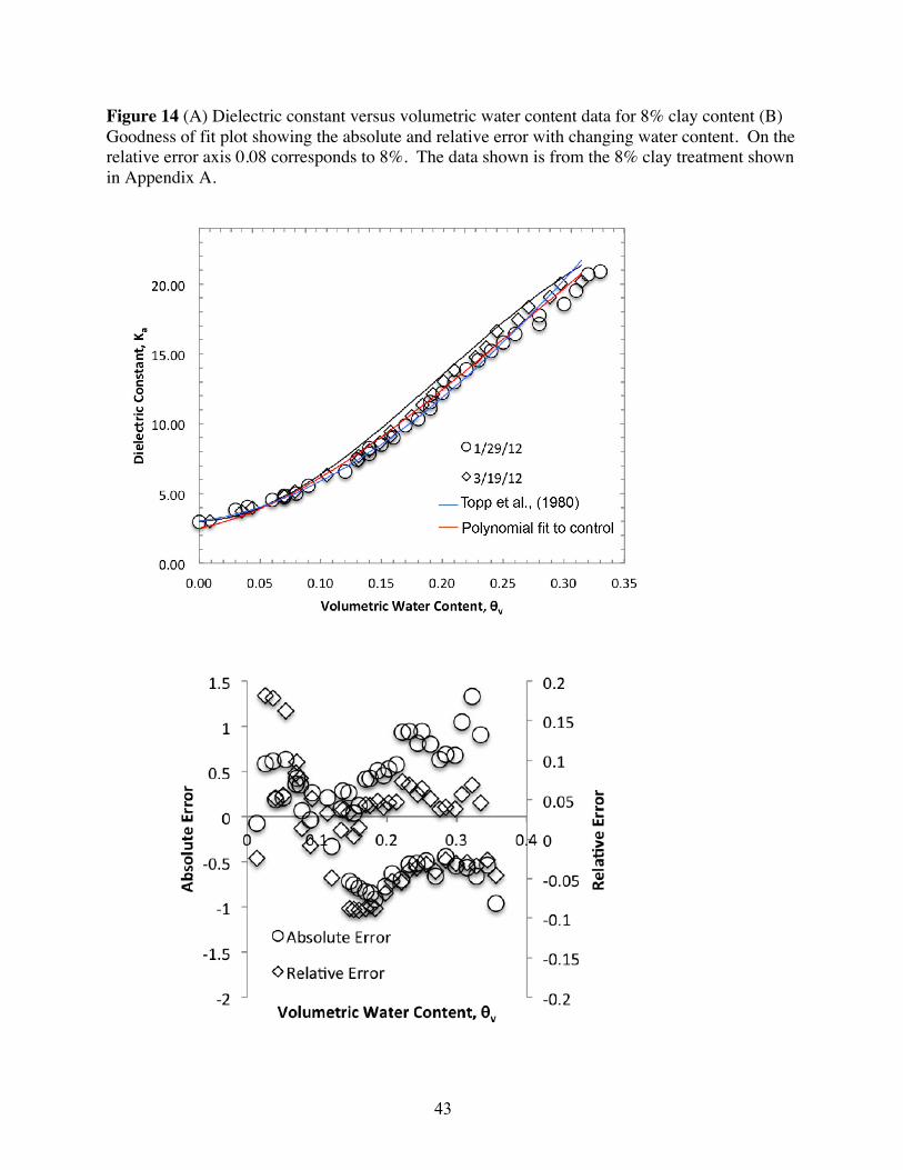
Figure 14 (A) Dielectric constant versus volumetric water content data for 8% clay content (B) Goodness of fit plot showing the absolute and relative error with changing water content. On the relative error axis 0.08 corresponds to 8%. The data shown is from the 8% clay treatment shown in Appendix A.

44

Figure 15. Third degree polynomials showing the relationship dielectric constant versus volumetric water content for quartz sands containing 0,2,4,6, and 8 weight percent clay content. Data is from all of the mixtures shown in Appendix A.

45

It has been suggested in previous studies that bound water controls the curvature of the

polynomials at low water contents. Bound water is a function of surface area, which is

controlled predominately by clay content and mineralogy. Therefore, it was expected that

increasing clay contents would lead to an increased contribution of bound water, leading to a

noticeable shift in the low slope region of the polynomials to the right (towards higher water

contents). The lack of a noticeable shift in the curves suggests that unknown factors, other than

bound water, are affecting the curvature of these polynomials at low water contents. The nature

of these factors is unknown.

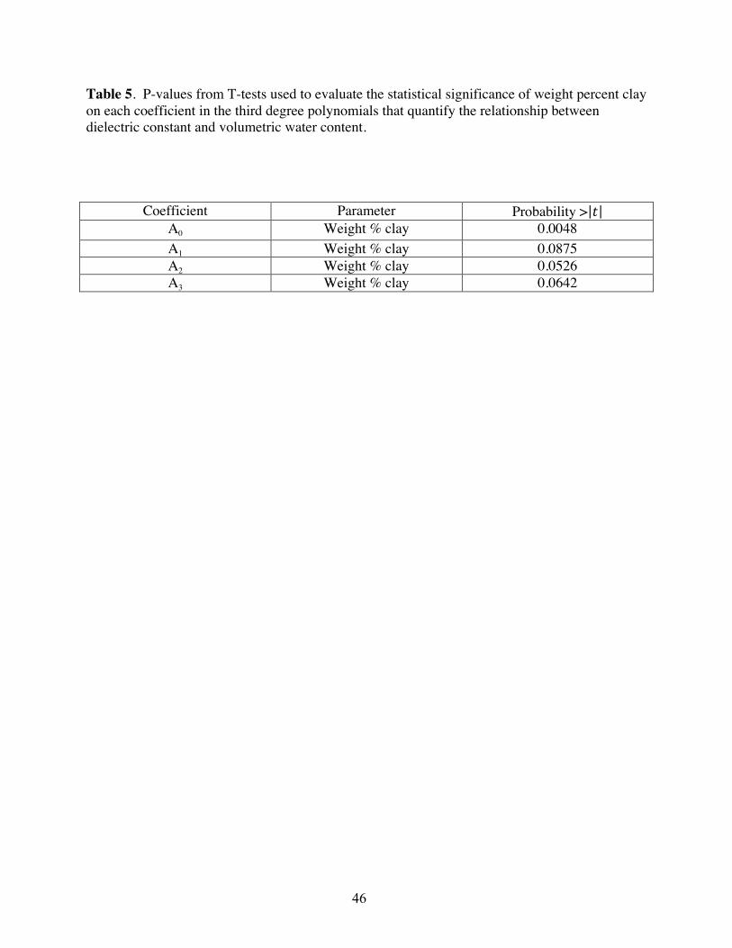
Previous studies have suggested the need for a parameter within dielectric models that

accounts for the contribution of clay. Thus, data from the clay content treatments were further

analyzed to take a more quantitative look at the differences between the polynomials fit to the

individual clay treatments. Bivariate fits were performed for each of the coefficients that make

up the individual polynomials versus clay content. The results of this analysis can be seen in

Figure 16 and Table 5. The bivariate fit results show that the clay content has a small but

statistically significant effect on the A0 coefficient of the polynomials fit to the data of the

quartz-clay mixtures. P values for the A1, A2 and A3 analysis show that there is a greater than 5

percent chance that there is no relationship between these parameters and clay content. These

results lead us to conclude that clay content has no effect on the curvature of the individual

polynomials. However, the results of the A0 analysis indicate that increasing clay content does

lead to small positive vertical displacement of the polynomials. In other words, clay content

affects the dielectric behavior of a material by contributing to the dielectric response at zero

water content. This result is not surprising considering the kaolin clay has a dielectric constant

of approximately 11 compared to the dielectric constant of the quartz sand, approximately four.

46

Table 5. P-values from T-tests used to evaluate the statistical significance of weight percent clay on each coefficient in the third degree polynomials that quantify the relationship between dielectric constant and volumetric water content.

Coefficient Parameter Probability > ! A0 Weight % clay 0.0048 A1 Weight % clay 0.0875 A2 Weight % clay 0.0526 A3 Weight % clay 0.0642

47

2.4  

2.5  

2.6  

2.7  

2.8  

2.9  

3  

3.1  

0   2   4   6   8   10  

A 0  

Weight  Percent  Clay  Content  

0  

5  

10  

15  

20  

25  

0   2   4   6   8   10  

A 1  

Weight  Percent  Clay  Content  

0  

50  

100  

150  

200  

250  

300  

0   2   4   6   8   10  

A 2  

Weight  Percent  Clay  Content  -­‐425  

-­‐375  

-­‐325  

-­‐275  

-­‐225  

-­‐175  

-­‐125  

-­‐75  

-­‐25  

0   2   4   6   8   10  Weight  Percent  Clay  Content  

A 3  

Figure 16. Bivariate fits for each coefficient A) A0 B) A1 (C) A2 D) A3 produced from the third degree polynomials by weight percent clay content.

P = 0.0048 P = 0.0875

P = 0.0526

P = 0.0642

48

Before evaluating the effect that clay content had on the A0 coefficient, a polynomial was

fit to all of the clay data (equation 18). The fit produced an R2 value of 0.985.

!! =   2.82   ± 0.13 + 10.72   ± 3.11 θ +   230.88   ± 19.74 θ! − (347.41   ± 35.24)θ! [18]

This R2 value indicates that the regression plot shows good correlation and explains essentially

all of the relationship between dielectric constant and water content. However, the bivariate fit

did indicate that clay content had a statistically significant effect on the vertical displacement of

the curves.

Following the bivariate analysis, all of the data for Ka versus both weight percent clay

content and volumetric water content were combined and regressed to produce a new third

degree polynomial that also accounted for weight percent clay content:

!! = 2.48   ± 0.14 + 12.12   ± 2.95   θ +   217.61   ± 18.80 θ! −   319.90   ± 33.66 θ! + 0.08(% clay) [19]

By including the weight percent clay content in the equation, the R2 value increased from 0.985

to 0.986.

5.4 Iron Oxyhydroxide Observations

The procedure for iron coating the sand grains produced grains with visible coatings and

a bright orange characteristic color of abundant ferric iron oxyhydroxide. The coatings change

the surface charge to produce a new solid-fluid interface that is typically a function of both the

underlying mineral grains and the coatings themselves (Hendershot, 1983). For example, the

point of zero charge (PZC) of pure quartz mineral surfaces is 2.2 (Parks, 1965). Conversely, the

PZC of iron oxyhydroxide coatings is 7.5-8.5 (Hendershot, 1983). In the rare case that there is

enough coverage to completely isolate the underlying quartz grains from the aqueous

environment we would expect the grain to act physically and chemically as an iron oxyhydroxide

solid (Iler, 1979). Scanning electron micrographs have shown that quartz surfaces usually have

49

contact with pore fluids through cracks and other imperfections in the mineral coatings

(Hendershot, 1983). Micrographs were not collected of the iron oxyhydroxide coated quartz

surfaces in this study, but would have been beneficial to show the extent of coatings and confirm

the contribution of the quartz and iron oxyhydroxide coatings to the overall surface charge. Here

we assumed that the surface coatings were not all encompassing and therefore expected the

surface charge behavior of the iron oxyhydroxide coated quartz sample, described by its PZC, to

be some intermediate between both the underlying quartz grains and overlying coatings.

The coatings produced for this study were stable and did not appear to separate from the

quartz grains during handling. However, trace amounts of iron usually came out of solution

during pumping as evidenced by a characteristic orange tint to the solution in the solution trap

flask. As with the clay treatments, initial subsidence of the sample was a common occurrence

when the samples were fully saturated. Again, any effect caused by the subsidence was assumed

to be constant between trials. In contrast to the clay treatments, there was no difference in

pumping time between the iron oxyhydroxide coated samples and the Control (pure quartz).

Hence, the iron data was collected more much more quickly than the clay content data in the

previous experiment.

5.5 Iron Oxyhydroxide Results The raw data collected for this analysis are provided in Appendix B. A third degree

polynomial (Figure 17) describing the relationship between dielectric constant and volumetric

water content was fit to the iron coated quartz sand data using the least squares regression

method. An R2 value of > 0.999 was obtained, indicating that this model explained essentially

all of the relationship between Ka and θ in the presence of iron coatings (Table 6).

50

Figure 17. (A) Dielectric constant versus volumetric water content for iron oxyhydroxide coated quartz grains. (B) Goodness of fit plot showing the absolute and relative error with changing water content. The data shown is from the iron oxyhydroxide coated samples shown in Appendix B.

51

Table 6. Summary of the polynomials produced from least square regressions for collected dielectric versus volumetric water content data for both pure quartz and iron oxyhydroxide coated quartz grains. Polynomials are shown in the form Ka = A0 + A1θ + A2 θ2 +A3θ3

Clay Content A0 A1 A2 A3 R2 Pure Quartz 2.51 ± 0.12 15.59 ± 2.86 163.42 ± 17.10 -183.08 ± 28.87 0.998

Iron Coatings 2.3 ± 0.00 24.8 ± 1.6q 120.2 ± 9.3 -131.4 ± 14.6 0.999

52

This study was focused less on quantifying the effect of iron coatings on the surface

charge of quartz grains than on how the surfaces charges of these new solid-fluid interfaces

affect the dielectric response of a iron oxyhydroxide coated quartz sand. As discussed above in

section 5.2, the Control data shows the two distinct regions in the polynomial that are believed to

represent the difference in the physical properties between bound and free pore fluid. At the pH

of most natural waters, and the pH of the samples measured in this study (6.25) pristine quartz

surfaces have a net negative charge and therefore are assumed to have the surface charge

conditions necessary to lead to this biphase distribution of water. However, the iron

oxyhydroxide coated quartz samples were expected to have a neutral to slightly positive charge

at the pH values measured in this study (≈4.3). This low net surface charge was expected to limit

the interactions of the mineral grain and pore fluid thereby limiting the effect that any bound

water would have on the dielectric response of the sample. However, from the graphs, we can

see that the Control and iron oxyhydroxide coated samples show similar behaviors across all

water contents. This suggests the coatings had little effect on the presence or contribution of

bound water compared to the effects that would be expected for pure quartz sands. Unlike the

clay treatments, if iron coatings had had an effect on the dielectric behavior of the quartz sands,

an extensive amount of additional investigation would be required to include a parameter within

the dielectric models to account for the iron oxyhydroxide coatings.

An examination of the results indicates that the dielectric responses of quartz-clay and

iron oxyhydroxide coated samples do not show the expected differences from the pure quartz

Control. This led the investigator of this study to revisit the assumptions that underlay the

hypothesis of this study. The original assumption of this investigation, as in previous studies,

was that the curvature of dielectric responses was influenced by the variable contributions of

53

bound versus bulk water. However, the clay and iron oxyhydroxide treatments, the two

parameters that we postulated to affect the contribution of bound water in porous materials had

no qualitative or quantitative effect on the curvature of the polynomials. Our observations and

the analysis of the Ka versus θv data suggest the classical explanation for the curvature of

dielectric responses may be incorrect. It appears that the shape of the curve is not dependent

upon bound water and thus, must be dependent on other unknown factors.

The interpretation that bound water does not control curvature at low water contents is

supported by four lines of evidence from the experimental conditions used in the experiments for

the Control, clay and iron oxyhydroxide treatments. Taking a closer look at the experimental

procedure, recall that that the addition of the air bubbler to the experimental design maintained a

film of bulk water that would have masked any contribution of bound water. Nonetheless, the

relationship between dielectric constant and water content in the Control is nonlinear. It is also

notable that the series of experiments that increased the clay content also increased the surface

area, which should have increased the proportion of bound versus bulk water, yet there is no

evidence for an extension in the low slope, “bound water,” region of the curves toward higher

water contents. The iron oxyhydroxide coatings have a higher PZC that should change the

structure of the bound water and the interactions with the surfaces of the quartz sand. However,

there was no significant change in dependence Ka versus θv. Finally, the responses from our

experiments and the relations reported in Topp et al. (1980) are not significantly different.

A calculation was performed to estimate the thickness of a monolayer of water and how

much a monolayer of water would add to the overall θv. The geometric surface area of a perfect

sphere was used in the calculation. It is believed that using the surface area of real grains would

increase the surface areas and therefore the water estimates by no more than one order of

54

magnitude. It was also believed that any effects coming from interference at the grain contacts

would lead to an error of less than one percent. The results of the calculation show that one

monolayer of water would be 3.1 Angstroms thick. Three monolayers of water would lead to a

water content of 5.57 x 10-6. Therefore at a volumetric water content of 0.01, there would be

approximately 5400 monolayers of water along the grain surfaces. The interpretation of these

results is that the presence of bound water at three monolayers is immeasurably small and could

not be the explanation for the shallow initial slope in the relationship dielectric constant versus

water content.

55

6. Summary

The results and interpretations of the study can be summarized in four points.

1. The experimental design maintained a film of bulk water that masked any contributions

from bound water. Despite this realization, the dielectric responses of the experiments do

not show a linear response. The behavior is similar to that reported in Topp et al., (1980).

2. The classical interpretation that the curvature of the dielectric responses is influenced by

the different contributions of bound versus bulk water appears to be incorrect. This

interpretation was used in three papers that are widely accepted and cited often

throughout the literature

a. Topp et al., (1980) Water Resources Research

“curve shapes gave qualitative confirmation of the hypothesis that the active surface area of the soil controls the dielectric properties of the first few molecular layers of water added to the soil.”

b. Wang et al., (1980), IEEE Trans. Geosci. Remote Sens.

“It is necessary to take into account the reduced dielectric behavior of the initially absorbed water.” “…for moisture contents below the transition moisture, the water in soils is thought to behave like ice and, consequently the dielectric constant for ice is used in the mixing [models].”

c. Hallikainen et al., (1985), IEEE Trans. Geosci. Remote Sens.

“…the dielectric constant of a soil mixture is, in general, a function of……the relative fractions of bound and free water….”

3. A properly designed study of bound water effects on dielectric response has not been

conducted. The proper design of such a study would require significant heating/drying to

remove bulk water as well as other specialized experimental techniques.

56

4. Most importantly, the classical interpretation of the nonlinear dielectric response of

porous media with changing water content needs to be revisited. This behavior cannot be

explained by a transition between contributions from bound versus bulk water. Further

investigation is needed to identify the physical basis for this behavior.

57

References: Atkins, P. W., 1978, Physical Chemistry, New York, New York, W.H. Freeman and Company. Birchak, J. R. (1974). "High dielectric constant microwave probes for sensing soil moisture." Proceedings of the IEEE 62(1): 93-98. Brantley, S.L. (2007). “Crossing Disciplines and Scales to Understand the Crtical Zone.” Elements (Quebec) 3 (5): 307-314 Chandler, D. G. (2004). "Field Calibration of Water Content Reflectometers." Soil Science Society of America Journal 68(5): 1501. Curtis, H.L., Defandorf, F.M. (1929). “Dieletric constant and dielectric strength of elementary substances, pure inorganic compounds, and air.” Washburn, E.D. (ed.), International Critical Tables of Numerical Data, Physics, Chemistry and Technology 6: 73-107 Davis, J. L., and Annan, A. P., 1989, Ground-penetrating radar for high-resolution mapping of soil and rock stratigraphy: Geophysical Prospecting 37, p. 531–551. Davis, J. L. and W. J. Chudobiak (1975). "In-Situ meter for measuring relative permittivity of soils." pp. 75-79. Dove, J.E., E.L. Haun, J.P. Seltzer, P.M. Dove. (In Preparatoin). “Silicification of Fine-Grained Soils.” Fellner-Feldegg, H. (1969). "Measurement of dielectrics in the time domain." Journal of physical chemistry (1952) 73(3): 616-623. Grantham, M.C., P.M. Dove, T.J. DiChristina (1997). “Microbially catalyzed dissolutoin of iron and aluminum oxyhyroxide mineral surface coatings.” Geochemica et Cosmochimica Acta 61 (21): 4467-4477 Hallikainen, M. T., F. T. Ulaby, et al. (1985). "Microwave Dielectric Behavior of Wet Soil-Part 1: Empirical Models and Experimental Observations." Geoscience and Remote Sensing, IEEE Transactions on GE-23(1): 25-34. Hendershot, W.H. (1983). “Effect of Sesquioxide Coatings on the Surface Charge of Standard Mineral and Soil Samples.” Soil Science Society of America Journal 47 (6): 1252. Hoekstra, P. and A. Delaney (1974). “Dielectric Properties of Soils at UHF and Microwave Frequencies.” Journal of Geophysical Research 79 (11): 1699-1708. Iler, R.K. (1979). The Chemistry of Silica Solubility, Polymerization, Colloid and Surface Properites and Biochemistry. Toronto, Canada, John Wiley and Sons.

58

Jacobsen, O. H. (1993). "A laboratory calibration of time domain reflectometry for soil water measurement including effects of bulk density and texture." Journal of Hydrology (Amsterdam) 151(2-4): 147. Kharadly, M. M. Z. (1953). "The properties of artificial dielectrics comprising arrays of conducting elements." Proceedings of the IEE - Part III: Radio and Communication Engineering 100(66): 199. Knight, R. A. Abad (1995). “Rock Water Interaction in Dielectric-Properties – Experiments with Hydrophobic Sandstones.” Geophysics 60 (2): 431-436 Night, R.A., L.J. Pyrak-Nolte, L. Slater, E. Atekwana, A. Endres, J. Geller, D. Lesmes, S. Nakagawa, A. Revil, M.M. Sharma, C. Staley (2010). “Geophysics at the Interface: Response of Geophysical Properties to Solid-Fluid, Fluid-Fluid, and Solid-Solid Interfaces.” Reviews of Geophysics Ledieu, J., P. Deridder, P. Clerck and S. Dautrebande (1986). “A Method of Measuring Soil-Moisture by Time Domain Reflectometry.” Journal of Hydrology 88 (3-4): 319-328 National Research Council (2000). Seeing into the Earth: noninvasive characterization of the shallow subsurface for environmental and engineering applications. Washington, D.C., National Academy Press. Olhoeft, G. R., 1989, Electrical properties of rocks; in, Physical Properties of Rocks and Minerals, Y. S. Touloukian, W. R. Judd, and R. F. Roy, eds.: New York, New York, Hemisphere Publishing Corporation, p. 257–329. Parks, G.A. (1965). “The isoelectric Points of Solid Oxides, Solid Hydroxides, and Aqeous Hyroxo Complex Systems.” Chemical Reviews 65 (2): 177-198 Pearce, C. A. R. (1955). "The permittivity of two phase mixtures." British Journal of Applied Physics 6(10): 358-361. Peplinski, N.R., F.T. Ulaby, M. Dobson (1995). “Dielectric properties of soils in the 0.3 – 1.3 – GHz range.” IEEE Transactions on Geoscience and Remote Sensing 35 (3): 784-787 Robinson, D.A., S.B. Jones, D. Wraith, S.P. Friedman (2003). “ A Review of Advances in Dielectric and Electrical Conductivity Measurements in Soils using Time Domain Reflectometry.” Vadose Zone Journal 2 (4): 444-475 Sabburg, J., J.A.R. Ball, N.H. Hancock (1997). “Dielectric behavior of moist swelling clay soils at microwave frequencies.” IEEE Transactions on Geoscience and Remote Sensing 35 (3): 784-787

59

Schwartz, B. F., M. E. Schreiber, et al. (2008). "Calibrating access-tube time domain reflectometry soil water measurements in deep heterogeneous soils." Soil Science Society of America Journal 72(4): 917-930. Schneider, J.M. (2009). “ Time Domain Reflectometry – Parametric study for the evaluation of physical properties in soils.” Canadian Geotechnical Journal 46 (7): 753-767 Topp, G. C., J. L. Davis, et al. (1980). "Electromagnetic Determination of Soil-Water Content - Measurements in Coaxial Transmission-Lines." Water Resources Research 16(3): 574-582. Wang, J. R. and T. J. Schmugge (1980). "An Empirical Model for the Complex Dielectric Permittivity of Soils as a Function of Water Content." Geoscience and Remote Sensing, IEEE Transactions on GE-18(4): 288-295.

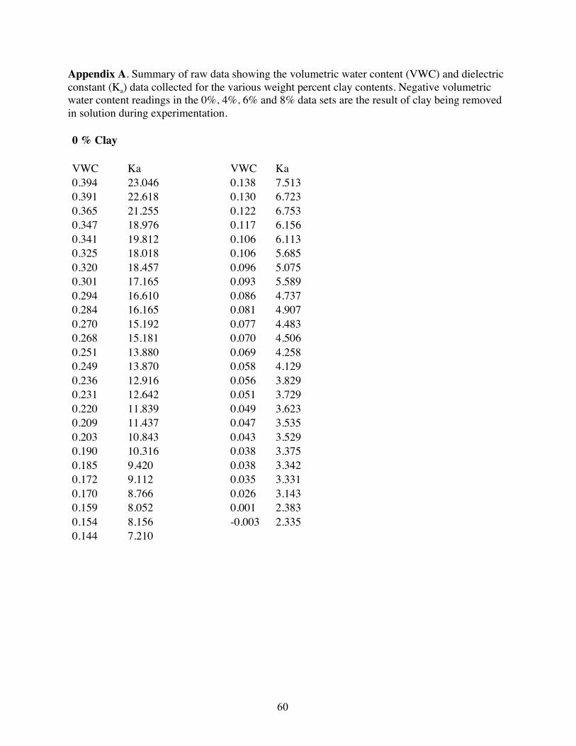
60

Appendix A. Summary of raw data showing the volumetric water content (VWC) and dielectric constant (Ka) data collected for the various weight percent clay contents. Negative volumetric water content readings in the 0%, 4%, 6% and 8% data sets are the result of clay being removed in solution during experimentation. 0 % Clay

VWC Ka

VWC Ka

0.394 23.046

0.138 7.513 0.391 22.618

0.130 6.723

0.365 21.255

0.122 6.753 0.347 18.976

0.117 6.156

0.341 19.812

0.106 6.113 0.325 18.018

0.106 5.685

0.320 18.457

0.096 5.075 0.301 17.165

0.093 5.589

0.294 16.610

0.086 4.737 0.284 16.165

0.081 4.907

0.270 15.192

0.077 4.483 0.268 15.181

0.070 4.506

0.251 13.880

0.069 4.258 0.249 13.870

0.058 4.129

0.236 12.916

0.056 3.829 0.231 12.642

0.051 3.729

0.220 11.839

0.049 3.623 0.209 11.437

0.047 3.535

0.203 10.843

0.043 3.529 0.190 10.316

0.038 3.375

0.185 9.420

0.038 3.342 0.172 9.112

0.035 3.331

0.170 8.766

0.026 3.143 0.159 8.052

0.001 2.383

0.154 8.156

-0.003 2.335 0.144 7.210

61

2% Clay

VWC Ka

VWC Ka

0.374 19.983

0.170 10.008 0.374 19.796

0.169 10.068

0.362 19.558

0.159 9.309 0.352 19.013

0.153 8.927

0.349 18.697

0.149 8.642 0.336 18.694

0.134 8.103

0.324 18.447

0.128 7.965 0.323 17.521

0.117 7.379

0.316 17.685

0.115 7.290 0.303 16.624

0.099 6.532

0.299 17.146

0.091 5.726 0.283 16.570

0.091 6.155

0.280 15.522

0.080 5.251 0.279 16.184

0.079 5.549

0.268 15.667

0.074 4.929 0.257 14.292

0.070 5.274

0.254 15.041

0.067 4.982 0.237 14.315

0.067 4.637

0.231 13.148

0.056 4.298 0.229 13.381

0.051 4.183

0.215 12.690

0.049 4.100 0.211 12.102

0.024 3.369

0.206 12.158

0.018 3.273 0.202 11.623

0.015 3.169

0.193 11.201

0.002 2.616 0.183 10.912

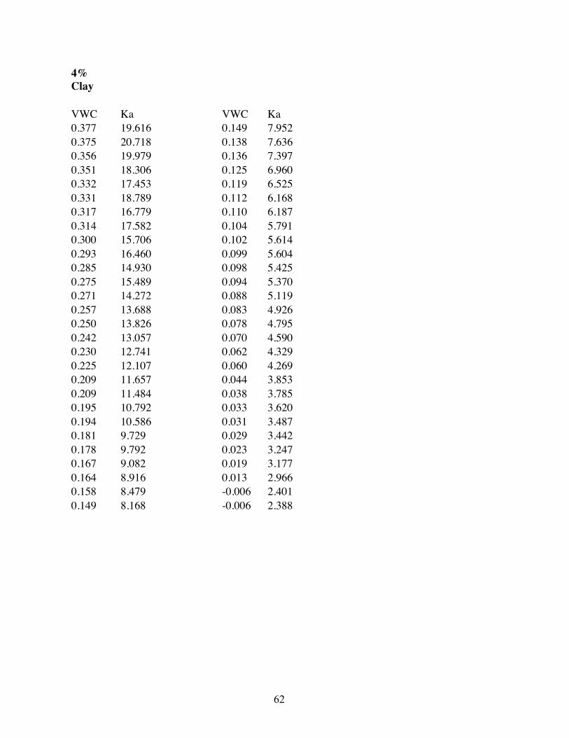
62

4% Clay

VWC Ka

VWC Ka

0.377 19.616

0.149 7.952 0.375 20.718

0.138 7.636

0.356 19.979

0.136 7.397 0.351 18.306

0.125 6.960

0.332 17.453

0.119 6.525 0.331 18.789

0.112 6.168

0.317 16.779

0.110 6.187 0.314 17.582

0.104 5.791

0.300 15.706

0.102 5.614 0.293 16.460

0.099 5.604

0.285 14.930

0.098 5.425 0.275 15.489

0.094 5.370

0.271 14.272

0.088 5.119 0.257 13.688

0.083 4.926

0.250 13.826

0.078 4.795 0.242 13.057

0.070 4.590

0.230 12.741

0.062 4.329 0.225 12.107

0.060 4.269

0.209 11.657

0.044 3.853 0.209 11.484

0.038 3.785

0.195 10.792

0.033 3.620 0.194 10.586

0.031 3.487

0.181 9.729

0.029 3.442 0.178 9.792

0.023 3.247

0.167 9.082

0.019 3.177 0.164 8.916

0.013 2.966

0.158 8.479

-0.006 2.401 0.149 8.168

-0.006 2.388

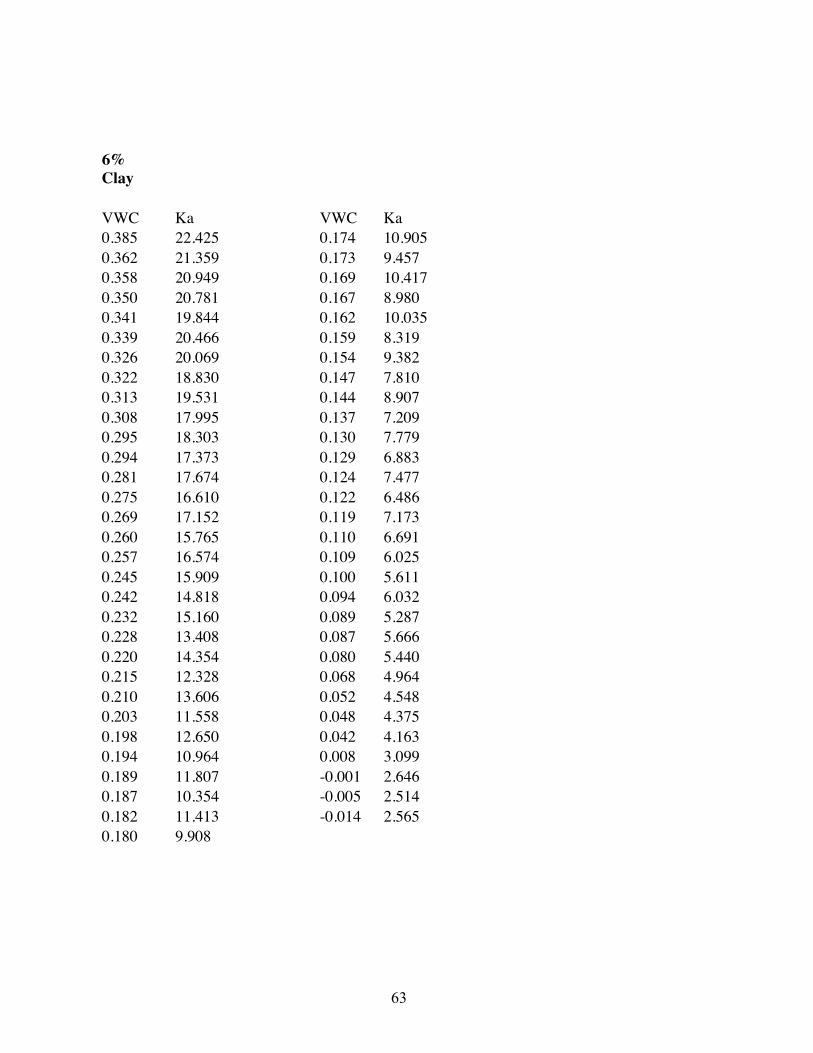
63

6% Clay

VWC Ka

VWC Ka 0.385 22.425

0.174 10.905

0.362 21.359

0.173 9.457 0.358 20.949

0.169 10.417

0.350 20.781

0.167 8.980 0.341 19.844

0.162 10.035

0.339 20.466

0.159 8.319 0.326 20.069

0.154 9.382

0.322 18.830

0.147 7.810 0.313 19.531

0.144 8.907

0.308 17.995

0.137 7.209 0.295 18.303

0.130 7.779

0.294 17.373

0.129 6.883 0.281 17.674

0.124 7.477

0.275 16.610

0.122 6.486 0.269 17.152

0.119 7.173

0.260 15.765

0.110 6.691 0.257 16.574

0.109 6.025

0.245 15.909

0.100 5.611 0.242 14.818

0.094 6.032

0.232 15.160

0.089 5.287 0.228 13.408

0.087 5.666

0.220 14.354

0.080 5.440 0.215 12.328

0.068 4.964

0.210 13.606

0.052 4.548 0.203 11.558

0.048 4.375

0.198 12.650

0.042 4.163 0.194 10.964

0.008 3.099

0.189 11.807

-0.001 2.646 0.187 10.354

-0.005 2.514

0.182 11.413

-0.014 2.565 0.180 9.908

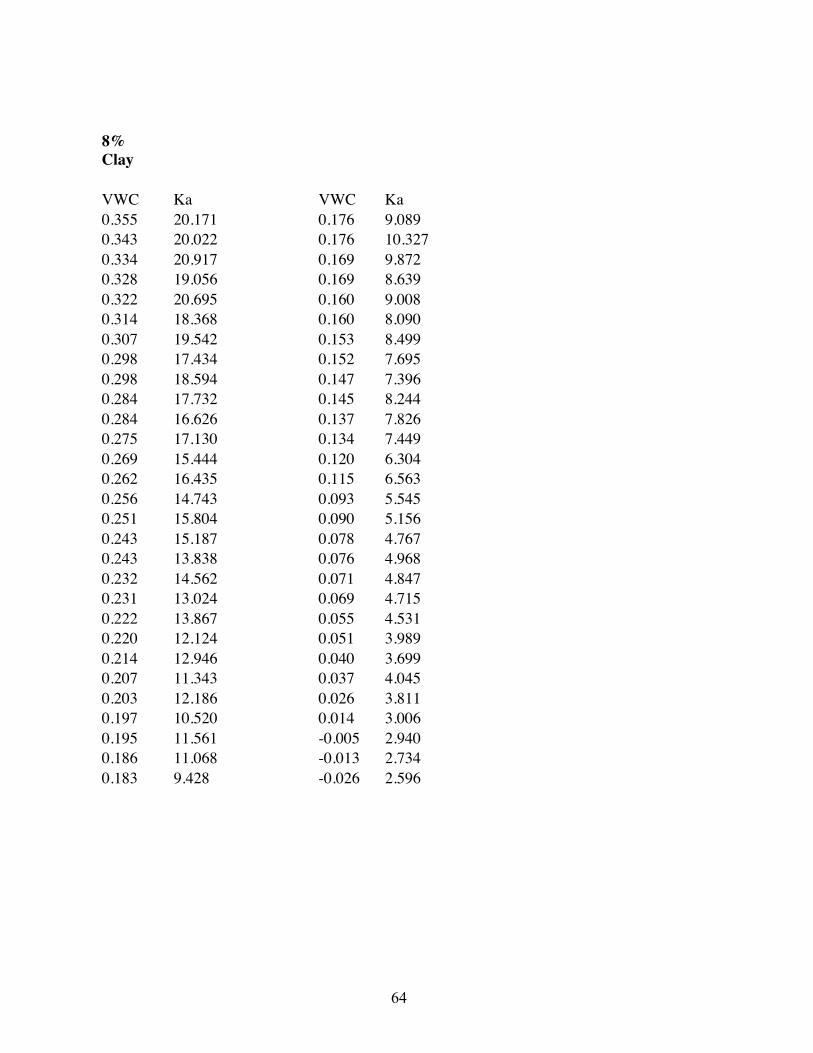
64

8% Clay

VWC Ka

VWC Ka

0.355 20.171

0.176 9.089 0.343 20.022

0.176 10.327

0.334 20.917

0.169 9.872 0.328 19.056

0.169 8.639

0.322 20.695

0.160 9.008 0.314 18.368

0.160 8.090

0.307 19.542

0.153 8.499 0.298 17.434

0.152 7.695

0.298 18.594

0.147 7.396 0.284 17.732

0.145 8.244

0.284 16.626

0.137 7.826 0.275 17.130

0.134 7.449

0.269 15.444

0.120 6.304 0.262 16.435

0.115 6.563

0.256 14.743

0.093 5.545 0.251 15.804

0.090 5.156

0.243 15.187

0.078 4.767 0.243 13.838

0.076 4.968

0.232 14.562

0.071 4.847 0.231 13.024

0.069 4.715

0.222 13.867

0.055 4.531 0.220 12.124

0.051 3.989

0.214 12.946

0.040 3.699 0.207 11.343

0.037 4.045

0.203 12.186

0.026 3.811 0.197 10.520

0.014 3.006

0.195 11.561

-0.005 2.940 0.186 11.068

-0.013 2.734

0.183 9.428

-0.026 2.596

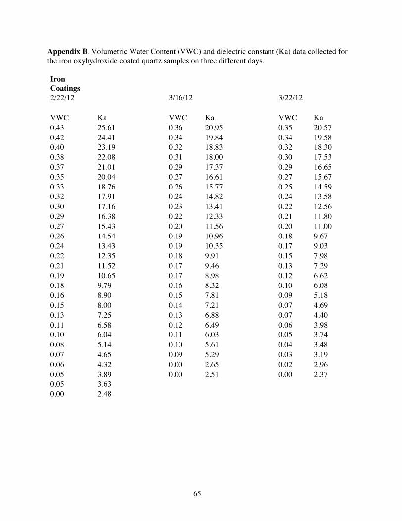
65

Appendix B. Volumetric Water Content (VWC) and dielectric constant (Ka) data collected for the iron oxyhydroxide coated quartz samples on three different days. Iron Coatings

2/22/12

3/16/12

3/22/12

VWC Ka

VWC Ka

VWC Ka 0.43 25.61

0.36 20.95

0.35 20.57

0.42 24.41

0.34 19.84

0.34 19.58 0.40 23.19

0.32 18.83

0.32 18.30

0.38 22.08

0.31 18.00

0.30 17.53 0.37 21.01

0.29 17.37

0.29 16.65

0.35 20.04

0.27 16.61

0.27 15.67 0.33 18.76

0.26 15.77

0.25 14.59

0.32 17.91

0.24 14.82

0.24 13.58 0.30 17.16

0.23 13.41

0.22 12.56

0.29 16.38

0.22 12.33

0.21 11.80 0.27 15.43

0.20 11.56

0.20 11.00

0.26 14.54

0.19 10.96

0.18 9.67 0.24 13.43

0.19 10.35

0.17 9.03

0.22 12.35

0.18 9.91

0.15 7.98 0.21 11.52

0.17 9.46

0.13 7.29

0.19 10.65

0.17 8.98

0.12 6.62 0.18 9.79

0.16 8.32

0.10 6.08

0.16 8.90

0.15 7.81

0.09 5.18 0.15 8.00

0.14 7.21

0.07 4.69

0.13 7.25

0.13 6.88

0.07 4.40 0.11 6.58

0.12 6.49

0.06 3.98

0.10 6.04

0.11 6.03

0.05 3.74 0.08 5.14

0.10 5.61

0.04 3.48

0.07 4.65

0.09 5.29

0.03 3.19 0.06 4.32

0.00 2.65

0.02 2.96

0.05 3.89

0.00 2.51

0.00 2.37 0.05 3.63

0.00 2.48