1

The Effect of Car Ownership on Employment:

Evidence from State Insurance Rate Regulation

[Job Market Paper – Preliminary and Incomplete]

C. Adam Bee*

University of Notre Dame

Department of Economics

ABSTRACT

Various economic theories suggest that one reason for low rates of

employment among low-skill, inner-city residents is that they are

spatially separated from jobs that have moved out to the suburbs. This

implies that if more low-skill urban dwellers owned cars, gaps in

employment rates would shrink. I exploit variation in state ―prior

approval‖ insurance rate regulation which has been shown to suppress

auto insurance prices, thereby decreasing the cost of owning a car. I find

that prior approval laws increase the proportion of multi-car households

among married couples with children. In those households, I find that

the additional car in the household encourages mothers to decrease their

labor supply while their husbands increase their labor supply. One

possible explanation of this result is that cars are stronger complements

to time spent in home production (and especially childrearing) than they

are to time spent in the labor market.

JEL Classifications: R23, R41, R49, J61, J64, J68

Keywords: Car ownership; Employment; Labor supply; Household time

allocation

* Department of Economics, University of Notre Dame, 434 Flanner Hall, Notre Dame, IN 46556. E-mail

cbee@nd.edu. I thank Bill Evans, Jim Sullivan, and the applied microeconomics faculty and seminar participants at

the University of Notre Dame. I also thank Jordan Theaker for excellent research assistance. This research has been

supported by an NSF IGERT-GLOBES Fellowship. I thank Robin Messina at AIPSO for providing residual market

data.

2

I. Introduction

A commonly cited barrier to employment among the urban poor is a lack of reliable transportation.

Previous attempts to test this conjecture have either focused on a small portion of the population (raising

concerns regarding external validity) or have used methods that are subject to reverse causality (raising

concerns about internal validity). Prior work has also ignored the role of intra-household allocations of

time and car access [so what? How is this a limitation?]. In this paper I address those limitations and

measure the effect of household car ownership on the employment of its members by exploiting a

previously overlooked source of exogenous variation in the cost of car ownership: changes in state-level

insurance rate regulation.

Studies of insurance regulation show that insurance rates tend to be lower in states that require

insurers to obtain ―prior approval‖ from the state insurance commissioner before implementing rate

changes. Using Consumer Expenditure Interview (CE) Survey data from the period 1984-2006, I find

that while rate-suppressing insurance regulation has no impact on whether a family owns a car, regulation

generates a two-percentage-point increase in second-car ownership rates. This effect is concentrated

among married parents of young children.

Although the CE Survey is the largest survey of car ownership available over a long period of time,

it is still too small to identify a reduced-form relationship between rate regulation and labor supply, so I

utilize data from the March Current Population Survey (CPS) to construct a two-sample instrumental

variables (2SIV) estimate of the effect of car ownership on labor supply.

Just as the effect of rate regulation on car ownership is driven by married couples with children in the CE

Survey, the association between rate regulation and employment is strongest among married couples with

children in the CPS.

Interestingly, I find that the ownership of the second car in the household has divergent effects on labor

supply within these households. I find that the second car increases the father‘s probability of

employment, while it decreases the employment of mothers. This result stands in contrast to the previous

literature on urban labor markets, which uniformly predicts that easing spatial frictions will increase labor

supply.

Since the effect is driven by parents of young children, one potential explanation of this result is that

cars are not only useful for getting to work, but they also increase the productivity of time spent in

household production. As I demonstrate below, mothers are disproportionately responsible for family-

3

related vehicle trips related to family activities, especially for child care purposes, and this disparity is

larger in families that own a second car.

This paper is part of a larger literature linking transportation to job market success. This literature

began with Kain‘s (1968) seminal work on the ―spatial mismatch hypothesis,‖ which argued that

persistent inner-city unemployment is a result of racial discrimination in housing markets, effectively

separating minorities from fast-growing employment opportunities in the suburbs. In the mid-1990s an

offshoot of this work called the ―automobile mismatch‖ claimed that insufficient access to a private

automobile is also an important spatial barrier to employment, especially for minorities.

It is easy to motivate the automobile mismatch hypothesis in that employment rates are much lower

for those who do not own a car. Some proponents of this hypothesis have called for programs to

subsidize car ownership in order to increase labor supply.1 Despite these claims, the basic correlation that

motivates the hypothesis is potentially contaminated by reverse causation. Employed individuals have

more income and are thus more able to afford a car than the unemployed.

For this reason, a subset of the automobile mismatch literature examines whether exogenous changes

in the cost of car ownership also alter employment. I contribute to this subset of the literature in the

following two ways. First, given the difficulty in finding exogenous variation in car ownership to identify

the models, many studies are forced to restrict their analysis to case studies with potentially limited

generalizability. I address those concerns and measure the effect of car ownership on employment in a

nationally representative sample by exploiting a previously overlooked source of exogenous variation in

the cost of car ownership: changes in state-level insurance rate regulation.

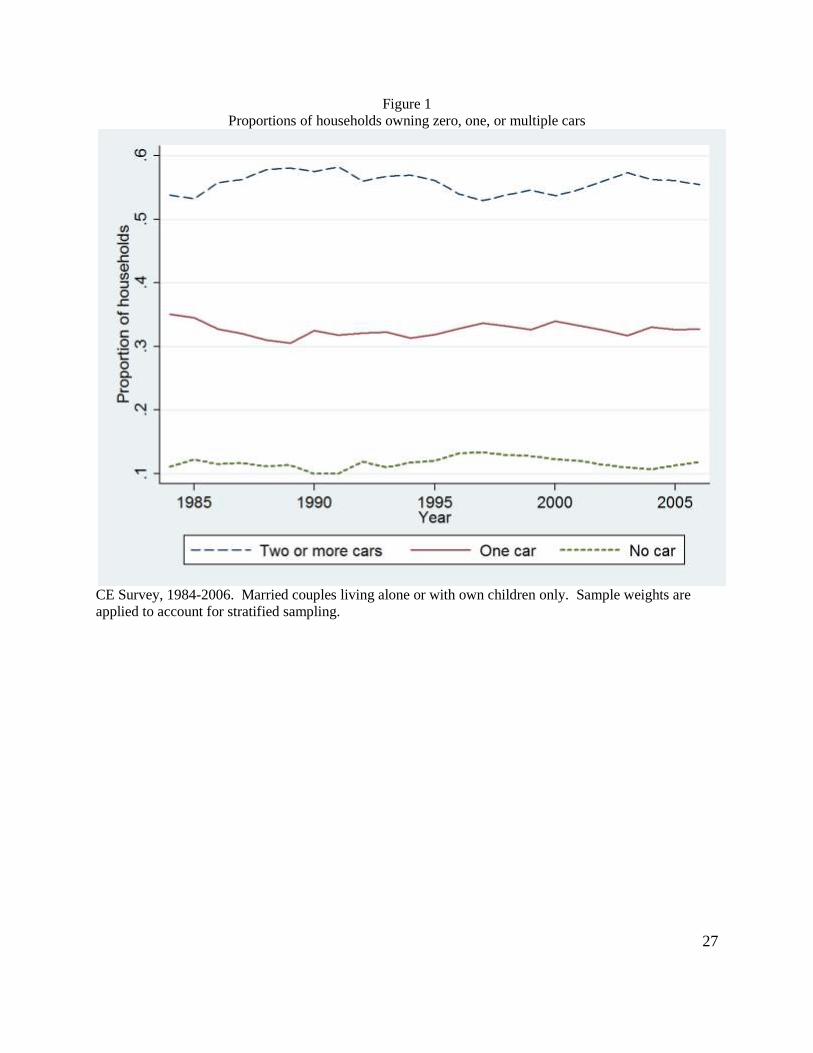
Second, previous studies have focused only on individual employment and primary car ownership,

presuming that the main effects of reducing the costs of car ownership will be to reduce the prevalence of

carlessness and to increase labor supply. The price elasticity of cars is greater at the second car than at

the first, however, and the proportion of households without a car is small and relatively stable over time,

as shown in Figure 1. The labor supply of secondary earners is also more elastic than that of primary

earners.

This paper‘s focus on how the second automobile impacts intra-household allocation of time is

unique in this literature. Since multiple-car ownership and secondary labor supply are both more elastic

to price, policies that change the costs of owning cars (e.g. environmental policies, infrastructure

investment, tort reform, etc.) will have their largest effect on these margins. Cars are generally shared

1 These include Smeeding (1993), Ong (1996), O‘Regan and Quigley (1998), Ong and Blumenberg

(1998), and Raphael and Stoll (2001), among others.

4

within households, but not equally across members; the second car reduces spatial frictions for secondary

earners by more than the first car does. Since secondary earners in low-income households can account

for a significant proportion of their households‘ wage earnings (Cattan, 1998), policies affecting

secondary car ownership may be particularly important to the well-being of families in poverty. Even if

one is only interested in primary labor force participation, estimates can be biased in specifications

neglecting the simultaneity of intra-household allocations of car access and time.

The literature‘s focus on how vehicles lower the spatial barriers to employment overlooks the

usefulness of vehicles in home production, and thereby misses an avenue through which car ownership

can alter labor supply. Much of home production is now accomplished outside the home, so a private

vehicle can dramatically increase the productivity of time spent in household production, encouraging exit

from the workforce. If policies affecting car ownership have their largest effects on secondary cars and

secondary earners, a consideration of household production may be crucial in understanding the effects of

those policies.

The rest of the paper is organized as follows. The following Section II provides some background

on the previous literature concerning transportation barrier to work, as well as the relevance of multiple-

car ownership for household time allocation. Section III describes the data used in this study, and

proposes a new source of exogenous variation in the cost of car ownership. State auto insurance rate

regulation lowers the cost of car ownership by suppressing insurance premiums. If car ownership rates

improve access to employment, then in reduced-form models we should see an increase in employment in

states after cost-reducing auto insurance legislation is passed. Section IV presents the results of the

analysis. Section V discusses other sources of exogenous variation, some of which have been previously

used in previous studies on this question. I find that they are unfortunately too weak to be useful as

instruments in the context of the CE Survey. Section VI concludes.

II. Background

II.A. Previous Literature Linking Transportation to Work

A commonly cited barrier to employment among the urban poor is a lack of reliable transportation.

The argument suggests that as metropolitan areas continue to sprawl outward, inner-city residents find

themselves more spatially isolated from high-growth areas because the transit systems they rely on are

increasingly unable to connect inner-city low-skill labor with vacancies scattered throughout low-density

suburbia.

5

This is not a new concern. Kain (1968) was the first to propose this ―spatial mismatch hypothesis‖

which suggested that a major explanation for low rates of employment among low-skill, inner-city black

residents in Chicago and Detroit is that racial discrimination in housing markets restricted them from

changing residential location to match the outward movement in the spatial distribution of low-skill labor

demand from the central cities to the suburbs.

Since Kain‘s seminal work, the hypothesis has been generalized to attribute residential concentration

of Hispanics as well as blacks to housing discrimination in US cities at large rather than just Chicago and

Detroit (e.g. Raphael and Stoll, 2001). Kain (1968) documents the shift in the location of manufacturing

establishments, but low-skill labor demand has shifted from manufacturing to the service and retail

sectors, which have grown faster in the suburbs than in central cities (e.g. Stoll et al., 2000). A large

literature developed that is dedicated to testing this more generalized spatial mismatch hypothesis, and

more generally whether spatial frictions can help explain persistently high unemployment in US central

cities.

From the beginning authors in this literature noted that spatial separations must be mediated by mode

of transportation—the implied mechanisms regard distance as relevant only insofar as it affects time,

whether spent searching or commuting. It was not until the mid-1990s, though, after consensus had not

been reached regarding the relevance of housing discrimination, that authors began to focus on mode as a

distinct explanation. Raphael and Stoll (2001) document wide disparities in car ownership across racial

and ethnic groups, comparable in magnitude to gaps in home ownership rates. Taylor and Ong (1995)

note that commuting distances were similar across races, compared to the wide dispersion in commuting

times associated with differences in transport mode.

Given the dearth of clear evidence regarding the special mismatch hypothesis, the academic

discussion has moved towards an analysis of mode choice. The offshoot ―automobile mismatch‖ 2

hypothesis emphasizes that the low densities of suburbs imply every residence is far from every

2 Automobile mismatch is also sometimes known as modal mismatch or transportation mismatch. Some

authors regard the automobile mismatch concept as a subset of the spatial mismatch hypothesis,

interpreting the spatial mismatch hypothesis to be the idea that commuting costs cause unfavorable labor

market outcomes. Blumenberg and Manville (2004) and Grengs (2010) provide extensive surveys, both

with this view. Taylor and Ong (1995) coin the phrase ―automobile mismatch‖, and they regard it to be

mutually exclusive of the spatial mismatch hypothesis, finding that the commuting patterns of blacks and

Hispanics in segregated neighborhoods are similar to those of suburban whites, conditional on car

ownership. In this paper I adopt the moderate view of Raphael and Rice (2002), among others, treating

the two conjectures as independent apart from their mutual concern with spatial frictions in urban labor

markets.

6

workplace; no matter where one lives in a metropolitan area, a car is essential for finding and keeping a

job.

Anecdotal evidence supports the idea that cars are necessary whether a family lives in the suburbs or

in the city. As part of the Moving to Opportunity (MTO) demonstration program, public housing resident

were experimentally relocated to lower-poverty area. Evaluations find no impact on the employment

levels of experimental households (Kling et al., 2005; Kling, Liebman, and Katz, 2007).3 In subsequent

interviews with relocated households, lack of personal transportation is a commonly cited impediment to

employment (Turney et al., 2006)4:

―Terry, a 33-year-old experimental, discusses how transportation issues often

result in her being late to her job as a school nurse at an elementary school in

Baltimore. ‗The bus driver, she was late one day and then the next day she

didn't come at all. … I am at the point where I am ready to buy a car,‘ she

says, but gets depressed because she cannot afford car insurance.‖

Many policies change the cost of driving; if car ownership is a key missing ingredient to economic

success, such policies may have unintended effects on labor markets. For example, many means-tested

transfer programs assess personal automobile assets when determining eligibility, including TANF and

SNAP5 (Sullivan, 2006; Bansak, Mattson, and Rice, 2010; Baum, 2009; Super and Dean, 2001), possibly

decreasing the incentive to own a car and hence, reducing employment prospects. Likewise, emissions

regulations, fuel efficiency requirements, and gasoline formulation standards all make owning an older

used car more expensive. Even the government‘s recent involvement in the auto industry itself can have

effects on car ownership, as the ―Cash for Clunkers‖6 program may have increased the prices of used cars

by requiring that cars traded in for credit be permanently disabled, reducing the supply of such vehicles.7

3 Quigley and Raphael (2008) reassess this assessment. Estimating a structural model of spatial mismatch

for comparison, they argue the experimental variation in neighborhood characteristics effected by MTO

was too small to generate enough statistical power to reject small or moderate effects on employment

levels. 4 The interviews were conducted in Baltimore, however, and the authors report that the health care jobs in

which half the employed experimentals reported working were more likely to be located in the city of

Baltimore than in the surrounding counties. 5 Temporary Assistance to Needy Families (TANF) was the replacement for the Aid to Families with

Dependent Children (AFDC) welfare program. Supplemental Nutrition Assistance Program (SNAP) is

the new name for the Food Stamps Program. 6 ―Cash for Clunkers‖ was renamed the Car Allowance Rebate System. From July 27 to August 25, 2009

vehicles under 25 years old getting <18 miles per gallon (or heavy trucks of any fuel economy older than

2001) could be traded in for scrap value and a $3,500-$4,500 voucher towards a new vehicle with a base

price under $45,000 and with a minimum fuel economy (22 mpg for passenger automobiles). 677,842

vehicles were scrapped and $2.85 billion was paid in credits. Other countries as well as Texas and

7

The most direct policy intervention, perhaps, is in the form of subsidies for highways and transit,

which change the relative prices faced by households choosing between private and public transportation.

Glaeser, Kahn, and Rappaport (2008) provide evidence from the 1980, 1990, and 2000 Censuses that new

mass transit stations induce the relocation of low-income, low-skill residents to its neighborhood.8 This

suggests that for many poor households, the cost of relocating can be lower than the cost of car

ownership, so disparities in car ownership are an important source of the residential segregation observed

by Kain and others. Holzer, Quigley, and Raphael (2003) document that when the heavy rail system was

expanded east of Oakland to high-growth, predominantly white suburbs, firms located near new stations

soon increased their hiring of minorities. These results can be interpreted as evidence against the

residential location choice frictions required by the spatial mismatch hypothesis in favor of the

importance of disparities in car ownership rates for explaining the persistent unemployment of urban,

low-skilled workers.

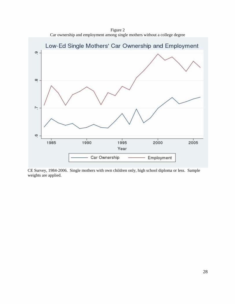
Early studies documented strong, positive, robust correlations between employment and car

ownership, showing that those who own cars are much more likely to be employed. Figure 2

demonstrates that for single mothers with less than a college degree, the time-series of car ownership and

employment are highly correlated. Interpreting this relationship is difficult because car owners are not

randomly selected in the population. Employed individuals have more income and are thus more able to

afford a car, so the correlation between the two variables may be due to causation in the opposite

direction—i.e., perhaps employment allows one to buy a car. This possibility is likely reflected in Figure

2 in that the enactment of welfare reform in the mid-1990s increased work for low-educated single

mothers. Alternatively, a third unobserved variable could affect both car ownership and employment in

the same direction, leading to a spurious correlation. For example, documentation of legal immigration

status may help one both in buying and financing a car and in obtaining employment.

Policy tools for ameliorating spatial mismatch can vary along three dimensions: community

development (moving jobs to inner city), residential mobility (relocating low-skill workers out to jobs),

and transportation programs (decreasing the reverse commuting costs of inner-city workers). The third of

California had previously implemented similar programs (http://www.cars.gov/files/official-

information/CARS-Report-to-Congress.pdf). 7 Anecdotally, recent news reports claim that prices for used cars have jumped as much as 30% year-on-

year in 2010, especially among low-mileage trucks and SUVs. A portion of this increase is probably due

to the recession‘s effect on household income, as used cars are inferior goods. 8 Turney et al. (2006) also report that many MTO experimental interviewed soon moved out of their

restricted, low-poverty, placement neighborhoods into poorer neighborhoods in order to be closer to bus

and train lines that ran more frequently.

8

these can be split further divided between mass transit subsidies and subsidies for car-centered

development. Connecting workers to jobs has long been a goal of transit, but many authors have claimed

that the nature of sprawl requires personal transportation. On the basis of ordinary least squares (OLS)

estimates, several authors have called for subsidies for car ownership among the poor (Ong, 1996; Ong

and Blumenberg, 1998; O‘Regan and Quigley, 1998). Smeeding (1993) suggests ―car stamps,‖ vouchers

that recipients can put toward the price of a car. TANF regulations explicitly allow for local authorities to

use TANF funds for ―Wheels to Work‖ programs, and such programs are now operating in a majority of

states (Goldberg, 2001).

Several studies focus on the causes and consequences of car ownership for welfare recipients, as the

shift from AFDC to TANF put greater emphasis on increasing recipients‘ labor force participation. In a

survey of TANF recipients in Los Angeles County, Ong (2002) finds that insurance premiums vary

substantially across geographic regions. He then demonstrates that car ownership is lower and

joblessness higher in high premium areas. Other papers exploit plausibly exogenous state-by-state

slackening of the vehicle asset tests in the AFDC and TANF welfare programs, a strategy that potentially

identifies a treatment effect of car ownership. Sullivan (2006) finds in the Survey of Income and Program

Participation (SIPP) that vehicle asset exemptions had a measurable effect on the probability of welfare

recipients owning a car, and Bansak, Mattson, and Rice (2010) find little evidence that it increased their

probability of employment. Baum (2009) uses the same methods in the National Longitudinal Survey of

Youth to identify a positive effect of car ownership on labor supply.

Raphael and Stoll (2001) use panel data from the 1991, 1992, and 1993 SIPP to estimate the

employment effects of moving to car ownership. They showed in a difference-in-difference framework

that the correlation between car ownership and employment was strongest for Blacks, moderate for

Latinos, and weakest for Whites, which mirrors the relative spatial isolation of these groups. They also

demonstrated that the correlation was strongest in cities with the highest indices of segregation. They

concluded that differences in car ownership rates may explain differences in employment rates across

racial and ethnic groups.

Raphael and Rice (2002) is the only national study (beyond those aforementioned restricted to

welfare recipients) that attempted to isolate the impact of car ownership on employment using plausibly

exogenous variation in car ownership. The authors documented that states with lower insurance

premiums had higher rates of car ownership and higher employment rates, suggesting a causal

relationship between car ownership and employment. Unfortunately that paper utilized only cross-state

variation in premiums and car ownership rates to identify the model, possibly subjecting the model to an

omitted variable bias: states with high car ownership rates had lower insurance premiums.

9

II.B. Cars and Home Production

More than 80 percent of all vehicle trips taken are for non-work purposes, but most of the literature

on car ownership (and especially its effect on labor supply) has focused on the impact of car ownership

for commuting. Such a narrow focus on journey to work misses the important role of the automobile in

home production. Expanding the model of time allocation to include home production changes the

prediction of the impact of a decline in the cost of car ownership on labor force participation from being

unambiguously positive to being ambiguous. The sign of the effect instead depends on how much car

access reduces the fixed time cost of going to work compared to how much it increases the marginal

productivity of time spent in home production.

II.B.1 Motivating Conceptual Framework

A unitary model of household decision making, with identical workers and diminishing marginal

utility in consumption and leisure, will imply that the optimal time allocation is identical between

household members.

Suppose that the household pays a fixed time cost for each member that works, in order to represent

time lost commuting. If both members work, the household pays a higher cost than if one household

member works. This fixed cost creates a non-convexity in the household‘s budget set, such that for some

preferences it is optimal for one worker to incur the commuting cost and work outside the home, and for

the other to avoid the commuting cost by withdrawing from the labor market. For any given set of

preferences, higher commuting costs have an unambiguously non-positive effect on the extensive margin

of labor supply (although for the remaining worker the effect on hours is ambiguous).

As is typical in home production models, suppose that the final consumption good is produced by

combining two intermediate goods: market wage earnings and home production. The first of these

intermediate goods is income collected from time spent in the labor market. The other intermediate good

is produced with time spent in home production, combined with household capital inputs like housing,

appliances, tools, and cars.

Mode choice can be introduced by allowing the household to exchange some of the market

intermediate good to buy a car, which enters into the household‘s production function in two ways. The

first way is that is decreases the fixed time cost of labor force participation. The second way is that it

increases the marginal productivity of time spent in home production. A change in the price of cars

10

affects the optimal time allocation through both channels, but the sign of that impact is ambiguous.9 The

key implication is this: If cars‘ elasticity of substitution with time spent in home production is sufficiently

small, and the factor by which cars reduce commuting time is also small, then lower car ownership costs

can increase the specialization of workers within a household.10

This view of car ownership fits into a large and growing literature on household time allocation and

the household production function.11

Some of these studies model capital inputs to the household

production function, but almost all of these assume capital is a substitute for time spent in home

production.12

The only paper I know of that explicitly allows for capital inputs to be complementary to

home production is Baxter and Rotz (2009). They examine the differential expenditure patterns of one-

and two-earner married couples to identify which roles different goods play in the household production

function. The authors note that a priori the theoretical effect of labor supply on car ownership is

ambiguous since the elasticity of substitution is unknown.

II.B.2 Empirical Facts

Women‘s access to reliable transportation may increase more with a family‘s second car than its

first. Noble (2004) measures the probabilities that each spouse will report being a ―main driver‖ of a

household vehicle, and finds that the difference between one- and two-car households in wives‘

drivership is 62 percentage points, an increase approximately equal to that between zero- and one-car

households for husbands‘ drivership.

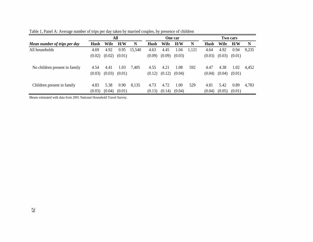
Table 1 illustrates a number of key points about the importance of cars as an input to both labor

supply and home production. This table reports results from the 2001 National Household Travel Survey

(NHTS). Conducted periodically by the U.S. Department of Transportation over the past 40 years, the

NHTS is the ―nation‘s inventory of personal travel.‖ Survey respondents provide data on all trips taken in

one 24-hour period in 2001, including the purpose of the trip, mode, time, place, and distance. If the trip

occurs in a personal automobile, data is also collected about all the occupants and vehicle characteristics.

9 As I document below, home production is now increasingly performed outside the home. Buying

groceries, picking up children from school, shopping, transporting children to doctors or activities, dining

at restaurants, etc., are all non-market activities which are often easier with a private automobile.

Splitting time spent in home production into two subcategories (inside home and away from home) yields

an unambiguous, testable hypothesis that a decrease in the price of a second car should increase the home

production done outside the home. Data availability prevents me from testing that hypothesis in this

paper. 10

This also depends on home goods being substitutes for market goods in the production of the final

consumption good (Jones, Manuelli, and McGrattan, 2003). 11

Aguiar and Hurst (2007) provide a survey of this literature. 12

Greenwood, Seshadri, and Yorukoglu (2005); Coen-Pirani, Leon, and Lugauer (2010); Cowan (1983).

11

Data is collected from 69,817 households and 160,758 people. I report results in Table 1 for married

couples living alone or with their own children only. Each column reports the mean number of trips by

car per day. In separate columns I generate results for three subsamples: all families, families with one

car, and families with two cars. For all subsamples I report separate estimates for husbands and wives

and I report the ratio of these two values and its standard error, which is calculated using the delta

method.

The numbers in the table generate the two key stylized facts about car travel outlined in the previous

section. The first fact is that a second car is correlated with wives‘ increased mobility while the second

fact is that the increased mobility afforded by the second car is associated with differential responsibility

for home production, and in particular differential responsibility for childrearing. When no children are

present, an extra car has no impact on the number of trips taken, whether by men or by women.

In Panel A of Table 1, I report average trips for families with and without children. Wives take 12%

more trips in multi-car families than in single-car, whereas husbands‘ trips are unchanged. In one-car

families without children males take 8 percent more trips than females, but in one-car families with

children there is no difference between genders. The basic results are unchanged in two-car families

without children, but note that in two-car families with children the number of trips for women increases

considerably to 5.4 trips per day and men are making 11 percent fewer trips per day, a difference that is

statistically significant at conventional levels.

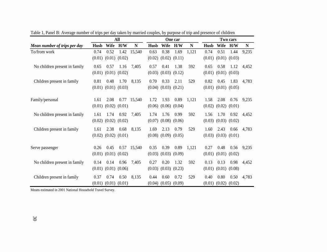
In Panel B I report the average number of car trips per day by purpose. I report results for three broad

purposes: driving to and from work, for family or personal reasons, and for serving particular passengers

in the car. This last group is a subset of family/personal reasons trips, and it includes trips like taking

children to soccer practice, doctor‘s appointments, or picking children up from school. Not surprisingly,

men are taking more car trips for work purposes in all family types and in one- and two-car families.

Among one-car families without children, there is no difference between husbands and wives in the

number of trips made for household care. However, this changes considerably by adding children or a

second car. In families with children and one car, husbands make 21 percent fewer trips for

family/personal reasons. In two-car families, husbands make 8 percent fewer trips without children in the

household but 34 percent fewer trips in households with kids.

Note that moving from one- to two-car families, wives without children are actually driving slightly

less (1.76 versus 1.70 trips per day). In contrast, wives with children are making 14 percent more trips in

households with a second car than wives in households with only one car. The second car only makes a

difference if children are in the house.

12

A large fraction of the family trips taken by both husbands and wives are serving a passenger in the

car. If no children are present, husbands and wives make similar numbers of these trips. With children,

however, wives are making many more of these trips. In households with both a second car and children,

wives serve as chauffeurs at double the rate of their husbands.

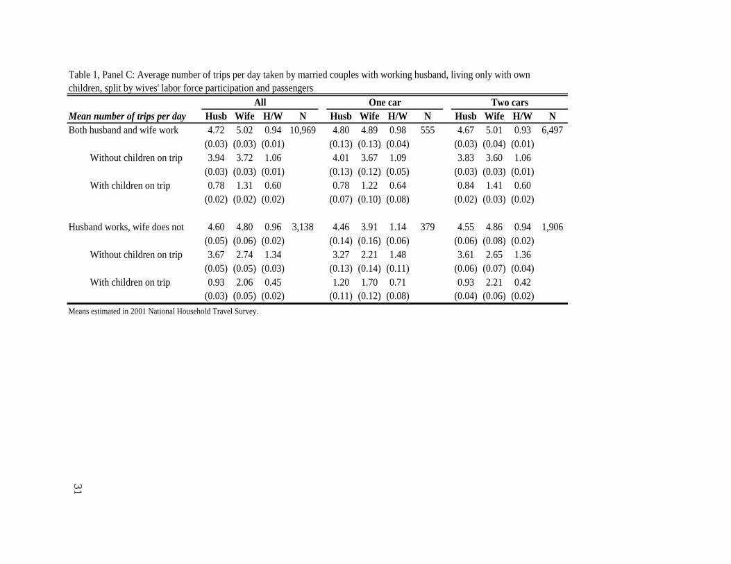
The importance of the second car for married mothers is most easily demonstrated in Panel C, where

I report estimates by the labor force status of the wife and by whether children are present in the car. In

this group of results, I include only households with children and in which the husband is employed. In

families where both parents work, the numbers of trips without children in the car are very similar for

both one- and two-car families. Notice however that in both one- and two-car families, men take about 40

percent fewer trips with children in the car than women take. For working mothers, the addition of the

second car is associated with a 16 percent increase in the number of trips with children (1.41 versus 1.22).

In households where the mother does not work, the addition of the second car is associated with a 30

percent increase in trips with children (2.21 versus 1.70). In households where both parents work, a

second car shifts both men‘s and women‘s trips toward children.

These results in Table 1 show that the positive association between multi-car ownership and

women‘s travel is much stronger when children are in the house. This interaction suggests that a second

car may be a complement to home production and may increase specialization in the household division

of labor. A decline in the cost of car ownership can reduce the cost of home production and encourage

exit from the workforce.

III. Methods and Data

In this section I examine the impact of car ownership on labor supply using arguably exogenous

variation in car ownership generated by state regulation of insurance rates. As I outline below, the

primary data set for car ownership is the Consumer Expenditure Interview Survey (CE Survey). This

sample has a number of distinct advantages, but it is a relatively small data set compared to many others,

and the fundamental cost of any two-step estimation procedure is a large reduction in precision. As a

result, I employ the two-sample instrumental variables method developed by Angrist and Krueger (1992,

1995) to augment the CE Survey with a much larger sample from the March Current Population Survey

(CPS).

III.A. Background on Auto Insurance Rate Regulation

Every state has an elected or appointed insurance commissioner whose job is to oversee regulation of

the insurance industry in that state. This devolution of regulation to the state level is the result of the

13

McCarron-Ferguson Act of 1945, which protected insurance cartels (―rating bureaus‖) from anti-trust

enforcement in exchange for increased regulation of the industry by the states. Over time states diverged

substantially in their chosen forms of regulation, ranging from direct, explicit price setting to near-total

deregulation.

Previous literature studying the impacts of these regulatory regimes has focused on one variable in

particular as a reliable measure of regulatory strictness. Whether or not a state requires each insurer to

obtain ―prior approval‖ from the state insurance commissioner before changing its rate structure

monotonically indicates the intensity of state regulation (Harrington, 2002). Szewczyk and Varma (1990)

show California‘s 1988 passage of a referendum enacting rate regulation was associated with significant

adverse effects on the share prices of firms with substantial exposure to the California market. Harrington

(1992) argues that state-specific, illiquid investments by insurers can be appropriated by state insurance

commissioners, such that exit by insurers will be too slow to deter rate suppression. D‘Arcy (2002) finds

that ―prior approval‖ is associated with larger assigned risk markets and more insurer insolvencies. Litan

(2001) surveys these and other analyses, concluding that the preponderance of the evidence supports the

hypothesis that ―prior approval‖ laws suppress rates below their competitive levels.

Table 2 shows the states in my sample that enact or repeal such rate-regulating legislation during the

sample period. These states are located in every area of the country, and the law changes are similarly

scattered across time periods. Some states enact ―prior approval‖ regulation while other states deregulate,

while still others have multiple regime changes. There does not seem to be any pattern to which states

change their regulatory regime in which years.

There are other aspects of state insurance laws that can potentially be used as variation in the cost of

car ownership. One is whether a state has a no-fault insurance system. Under no-fault, drivers and their

passengers are covered by the driver‘s own insurance regardless of who is at fault, and drivers have

limited ability to recover damages from other insured drivers. Previous research has demonstrated that

no-fault insurance changes the cost of insurance, but few states changed their compensation regimes over

the sample period, and preliminary investigations for this paper found that no-fault laws did not generate

enough variation in car ownership to identify the first stage.13

Rate regulation laws, on the other hand, may be more promising instruments. Although we cannot

rule out the possibility of the enactment of such laws depending on the macroeconomic condition of the

state, the inclusion of time effects would remove all but idiosyncratic shocks to the state, not shared by

the rest of the states in the sample for that year.

13 I further discuss no-fault laws and other potential sources of variation in Section VI.

14

III.B. Two-Sample IV Method

The goal of the paper is to examine the impact of car ownership on labor supply. As I outline below,

the data are repeated cross sections that vary over time and states, and the unit of observation is a

household. Therefore, the basic equation of interest can be described by a linear probability model of the

form

(1) Ehst = Ohst β1 + Xhst β2 + u1s + v1t + ε1hst ,

where Ehst is an indicator for the employment status of the head (or spouse, in some specifications) of

household h in state s responding in year t, Ohst is an indicator for whether the household owns a car, Xhst

is a vector of household characteristics (some of which are themselves member characteristics, such as

education of the head or age of oldest child). The three-part error structure captures fixed state (u1s ) and

year effects (v1t ) plus an idiosyncratic error (ε1hst).

OLS estimates of equation (1) are unlikely to produce consistent estimates of the impact of car

ownership on labor supply. One problem is omitted variable bias, in that some characteristics correlated

with both Ohst and Ehst are unobserved and thus omitted from Xhst.

Some of these omitted variables are obvious. For example, health and physical conditions such as

poor eyesight may make it difficult for an individual to obtain a driver‘s license and to work. Most

nationally representative data sets have limited ability to measure such covariates, and although I do have

a panel data set, the short time frame of the panel means there is not enough variation in car ownership

within the panel to exploit this dimension of the data.14

I can, however, control for any variables which are constant for all households within each state over

the time period by adding state fixed effects. This includes fixed attributes like the climate and

topography of the state, as well as the within-state averages of variables which do change over the period,

like average total highway lane-miles built or the typical political environment. I similarly control for any

unobserved macroeconomic shock within a given year, to the extent that it affects all states equally, using

year fixed effects.

Simultaneity bias, or reverse causality, is another potential problem. For example, having a job

provides one the income and access to credit necessary for buying and maintaining an automobile. These

14 I have at most four observations for each household. Each household is interviewed for consecutive

five quarters then rotated out, but the first interview is intended to set a baseline and is not reported.

Many households are interviewed for fewer than four quarters if they decline to continue to participate, if

they move to a new residence without informing the BLS, or if they leave the sample for any other

reason.

15

problems are essentially impossible to solve by adding covariates to the model. The only way to isolate

the causal effect of car ownership on employment is to either manipulate car ownership directly or to

isolate some variation in car ownership which is plausibly uncorrelated with the error.

Rate regulation laws may reduce the costs of car ownership, thus increasing ownership rates in states

that enact such laws. If rate regulation is to be a good instrument for identifying the effect of car

ownership on employment, it must only affect employment through car ownership itself. Since lower

prices increase the purchasing power of nominal wages, regulation may have an independent effect by

increasing real wages. Wage increases have an unambiguously positive effect on LFP in most models.

Motor vehicle insurance, however, represents 2.49 percent of the average household‘s expenditures,15

so

the average regulation-induced 11.23 percent decrease in annual premiums represents a 0.28 percent

increase in real wages. Such a small increase in overall price levels is unlikely to explain the observed

results.

Political endogeneity is another concern of this type. For example, states with unusually high rates

of unemployment may be more likely to enact a populist legislature willing to expand the scope of

government intervention in markets. If that state‘s unemployment time series has mean-reversion, then

such a political mechanism could yield spurious results. Political endogeneity could also occur if rate

regulation is enacted in response to particularly high insurance premiums, which themselves may have

been a result of a booming state economy (with high levels of employment, car ownership, vehicle miles

traveled, congestion, medical and repair prices, etc.)

Very few datasets contain each of the three variables (car ownership, employment status, and state-

year identifiers defining rate regulation) required for IV estimation. As mentioned above, the SIPP is one

of the few that do, but it covers a limited period of time. The CE Survey also measures all three, but even

across twenty years its sample is too small to detect an employment effect.

To solve this data availability limitation, I use the two-sample instrumental variables strategy (2SIV)

first developed by Angrist and Krueger (1992, 1995). The idea is to use one dataset to estimate the first-

stage effect of the instrument on the endogenous regressor, and use another dataset to estimate the

reduced-form effect of the instrument on the outcome of interest, which is assumed to work only through

the instrumented endogenous covariate. In this case, the first-stage equation is of the form

(2) Ohst = Rst π1 + Xhst π2 + u2s + v2t + ε2hst ,

15 In the December 2009 Consumer Price Index for Urban Consumers, the weight on motor vehicle

insurance is 2.492 percent. ftp://ftp.bls.gov/pub/special.requests/cpi/cpiri2009.txt

16

where all variables are defined as above and Rst is a dummy variable that equals unity if state s in year t

has prior approval legislation and zero otherwise. This equation will be estimated with data from the CE

Survey. The reduced form equation is defined as

(3) Ehst = Rst θ1 + Xhst θ2 + u3s + v3t + ε3hst ,

and the equation will be estimated with data from the March Current Population Survey. Finally, since

the model is exactly identified, the two-sample instrumental variables estimate is simply the ratio of the

reduced form estimate to that of the first-stage on the instrument Rst, or

(4) 1 1 1ˆ ˆ ˆ/ .

I derive standard errors for the 2SIV estimate by using a delta method technique developed by Dee and

Evans (2003).

III.C. Data

The CE Survey is a nationally representative, rotating panel survey administered quarterly by the

Bureau of Labor Statistics. Its main purpose is to provide the consumption bundle over which the

Consumer Price Index is computed to measure inflation. Each of approximately 7,600 addresses of

―consumer units‖, defined broadly as individuals who pool their incomes and make expenditure decisions

jointly, are interviewed for five consecutive quarters and then replaced. The first of the five surveys is a

reference survey so that new purchases are assigned to the correct quarter.16

The CE Survey data include expenditures that respondents could be expected to recall for three

months or more, household assets, and demographic characteristics of household members. Although

each household is interviewed on several occasions, I treat each year as a repeated cross-section of

households. Each observation represents one household‘s response in one quarter, so the number of

observations per household is equal to the number of interview responses.17

Since observations for each

household are likely to be highly correlated across time, unadjusted OLS standard errors would under-

estimate the variance of the distribution of the coefficient estimates. Accordingly, I adjust the standard

errors to allow for arbitrary correlation across observations within each state.

I combine data from survey years 1984 to 2006, generating panels of repeated cross-sections that

vary across consumer units, states, and years. I account for sample frame changes in 1986, 1996, and

16 Excellent descriptions of the CE Survey can be found in Meyer and Sullivan (2007), (2004), and

(2003). 17

Typically each household provides four responses, but a sizable fraction of households do not complete

all four surveys (after the initial baseline survey).

17

2006.18

Sampling weights were used in all regressions, although all of the results in this paper are

qualitatively similar when they are not used.

The CE Survey recodes state identifiers for some observations in order to protect respondent

anonymity. I drop any household with a recoded state identifier. In any state-year cell where recoded

state identifiers are not specifically flagged as such, all observations are dropped. About a quarter of the

sample (136,036 households out of 553,749) is dropped in this way. Table 11 shows the remaining

observations in each state-year cell.

Cars and market wage earnings are often shared within each household,19

so there is potential for

simultaneous determination of the labor supply of the primary and secondary earners within each

household. To capture these intra-household dynamics I focus on households consisting only of married

couples living alone or with only their own children.20

I count an individual as employed if he or she has been working for pay in the past twelve months. I

count personal vehicles for the purposes of household car ownership as cars, trucks, minivans, vans, or

sport-utility vehicles: motorcycles and mopeds do not count. Race and ethnicity variables assign ―white‖

and ―black‖ categories as non-Hispanic white and non-Hispanic black. Education variables have slight

changes at 1996. Before 1996, ―less than high school‖ is defined as anyone attending 11 years of school

or less; ―high school graduates‖ are anyone who has attended the 12th grade through three years of

college; and ―college graduates‖ are those who have attended four or more years of college. From 1996

onward, those who attended 12th grade but did not receive a diploma are categorized as ―less than high

school‖; ―high school graduates‖ include respondents with some college education but no degree and

anyone with an Associate‘s degree, and ―college graduates‖ are holders of Bachelor‘s degrees.

There are a few possibilities for reporting bias in the CE Survey. For example, when premiums

increase, many poor households may let their insurance coverage lapse and drive uninsured. Since this is

illegal in most states, these households may be reluctant to report that they own an automobile but will

have no such reluctance reporting their employment status. This effect will upwardly bias (in magnitude)

18 Specifically, the first quarter of each year‘s survey overlaps with the fifth quarter released in the

previous year. For example, the data for 1992 includes the four quarters of 1992 in addition to the first

quarter of 1993. Usually these overlapped quarters are identical, but in years in which the sampling frame

was changed, the two quarters can include different observations. I solve this by extracting all quarters

(including overlapping first quarters) and removing duplicated observations. 19

Indeed, the BLS defines a ―consumer unit‖ as a set of individuals sharing a substantial proportion of

household expenditures. 20

―Own children‖ include stepchildren and adopted children. Earlier versions of this paper did not

include this restriction, and the resulting estimates were similar to those produced here, though with

smaller confidence intervals. Those results are available from the author by request.

18

estimates of the effect of premiums on car ownership, and IV regressions of employment on car

ownership will be biased downward.

The Integrated Public Use Microdata Series - March Annual Demographic File and Income

Supplement of the Current Population Survey consists of 48 years (of which I use 23) of the Current

Population Survey (CPS), with its variable definitions harmonized across years. The CPS is collected

monthly by the Census Bureau and the Bureau of Labor Statistics, but the March Supplement is only

collected each March. Table 3 shows sample means for both the CE Survey and the CPS. Note that most

of the variables measured in both datasets have similar means.

The variable defining rate regulation laws in each state-year is drawn from the appendix of Grace

and Phillips (2008), who extend Harrington (2002). They categorize laws into eight categories of

regulatory strictness. Following Harrington (2002) I separate those into two categories, ―prior approval‖

and ―competitive rating‖. Prior approval laws range from the state explicitly setting insurance rates to

insurers at least needing the state insurance commissioner to have an option of disallowing rate changes

for some period between when the rates are filed with the state and when they are allowed to be used.

Competitive rating regimes, on the other hand, require insurers to file rate changes but then allow insurers

to use those rates without getting the approval of the state.

IV. Results: The Effect of Car Ownership on Employment

The incentives created by prior approval laws for households to buy their first car (or sell their last,

in the case of repeals) are too weak for prior approval to be a suitable instrument on the zero- to one-car

margin. Table 4 demonstrates that households appear unwilling or unable to buy their first car upon the

enactment of prior approval legislation. Across all groups, no first-stage estimate is statistically

significant.

This result is consistent with a few plausible explanations. One explanation is that cars are a

―lumpy‖ investment in that there are increasing returns to expenditures on a car at low levels of

expenditure, in part because there are sizable fixed costs to car ownership. Another possibility is that

there may be sizable transaction costs associated with changing one‘s level of consumption of cars (as in

Chetty and Szeidl, 2007). Whatever the reason, it appears that few households are sufficiently close to

the margin of car ownership to be induced by mildly cost-reducing policies to change their car ownership

status.

Married couples living alone are also shown in Table 4 to be just as unresponsive regarding their

decision to buy a second car as they are in the decision to buy a first car. Table 5, however, shows that

married couples living only with their own children buy an additional car when rate regulation goes into

19

effect. The first entry of the first column indicates that a ―prior approval‖ rate regulatory regime in a

given state and year is associated with a 2.4 percentage point increase in the proportion of households

owning two or more cars.

Rate regulation affects employment through its effect on car ownership. One might expect that this

effect is heterogeneous among different demographic subgroups, but the surprising result is that the effect

of rate regulation (through car ownership) is opposite for members of the same household. Following

along the first row, we find that rate regulation is associated with a 1.5 percentage point increase in male

labor supply and a 1.7 percentage point reduction in female labor supply. Without taking these offsetting

intra-household adjustments into account, the effects of car ownership on employment is obscured.

The 2SIV estimate indicates that a second car increases a husband‘s labor supply by 62 percentage

points. Given the sample mean, this implies a probability of employment well over 100 percent. The

corresponding effect of a second car on female labor supply is to reduce it by 70 percentage points. These

impossibly large estimates may be an artifact of the linear probability model specification, or they may

represent a deeper problem with the analysis.

The 2SIV results for women are consistently negative across suggest that car ownership reduces their

labor supply, but the adjusted standard errors are large enough that the null hypothesis cannot be rejected.

Table 5 also presents results for several subgroups. The effects appear to be widespread and

robust—it does not appear that one subgroup is driving the car ownership estimate while another group is

pushing the employment numbers. Although the 2SIV estimates for women in most subgroups are

lacking enough power to reject the null hypothesis at conventional confidence levels, they are consistently

negative.

Strikingly, the strongest results are among married couples with children under 16, as shown in

Table 6. This suggests that the gains from increased specialization may be partially due to the ability to

shuttle children to various activities. Once children can drive themselves (or the oldest child can partially

assume that role), the labor market effects of a second car are substantially diminished.

V. Alternate Specifications

The labor market effects implications of car ownership have been difficult to gauge, at least partially

because many events or factors which influence an individual‘s decision to purchase a car also affect an

individual‘s decision to work. For example, many states have reasonably strict emissions testing laws

that impose significant costs on owners of old, inexpensive cars. This may seem like a potential

candidate for exogenous variation in car ownership, especially since owners of such vehicles are likely to

be marginal car owners. Unfortunately state or local emissions testing laws are often a portion of a

20

package of air quality laws. These simultaneous policies can change the industrial composition of the area

and impact the skill distribution of labor demand.21

Other potential instruments, though, may plausibly satisfy the exclusion restriction but fail to have

any first-stage effect on car ownership. Tables 7 and 8 present first-stage results from several plausibly

exogenous determinants of car ownership, as estimated in the CE Survey with state and year fixed effects

and individual covariates. Columns (1) and (2) examines the role of compulsory insurance and no-fault

laws, respectively, using data from Cohen and Dehejia (2004).

Column (3) exploits variation in the proportion of car-years insured in the ―residual‖ or ―assigned

risk‖ markets for drivers who have been rejected at least twice on the private ―voluntary‖ market. Claims

in this assigned risk market are shared by all insurers operating in the state, and its size has been

consistently found to vary positively with regulatory strictness (e.g. Grabowski, Viscusi, and Evans,

1989). In that sense, it can be thought of as a continuous, ordinal index of the degree of regulatory

intervention, potentially providing more variation both across and within states.

The last four Columns (4) – (7) follow the method of Raphael and Rice (2002), the only previous

national study that addresses endogeneity. Gas taxes are obtained from the Department of Energy‘s

Petroleum Marketing Monthly, and measures of average premium expenditures are obtained from the

National Association of Insurance Commissioners. Unfortunately, I find no evidence of a first-stage

effect on car ownership at either the extensive or intensive margins. Together, these suggest an extremely

low price elasticity of demand for vehicles.22

VI. Conclusion

This study examines whether increased access to reliable transportation has an impact on the labor

supply of low-income, urban households. In particular, I focus on the potential implications of policies

altering the cost of driving for labor-market outcomes for the decision to buy a second car, and for the

decision of secondary earners to participate in the labor market. These secondary, intensive intra-

household margins have been previously overlooked in the related literature, but I argue that they are

important because these decisions are especially sensitive to policy choices.

21 Henderson (1996), Becker and Henderson (2000), and Greenstone (2002) are examples of relatively

recent work documenting the effect of the Clean Air Act on industrial composition. 22

Other possible instruments which I have investigated but do not report here include personal property

―wheel‖ taxes, presence of a 16-year-old age-eligible driver (compared to households with 15-year-olds),

and graduated driver licensing laws among households with teenaged children.

21

A concern with previous attempts using variation in the cost of car ownership to measure the impact

of car access on economic self-sufficiency is that costs are likely to be higher in areas with booming local

labor markets. In light of these reservations I assess one prominent variant of this approach, which uses

variation in the premiums paid for auto insurance. I find that this approach is almost entirely driven by

permanent cross-state differences, which raises the concern that unobserved permanent geographic

differences could cause this method to yield a spurious estimate.

To address this concern I explain some of these cross-state differences in premiums as a function of

insurance price regulation imposed by state governments. Eleven states substantially change the

strictness of their regulatory regimes in the study period, and I exploit these changes to isolate plausibly

exogenous variation in car ownership rates. In particular, I find that the proportion of households owning

two or more vehicles increases in states and years in which insurers are required to submit any proposed

rate changes to the state insurance commissioner for approval before instituting them in the market. This

result has potentially important policy implications in itself, as these laws are generally not directly

intended to change car ownership rates.

I find in the reduced form that these stricter regulatory regimes are also associated with an increase

in men‘s labor supply and a decrease in women‘s labor supply. Since insurance regulatory regimes could

only affect employment through its effect on car ownership, I interpret the ratio of these estimates as the

effect of car ownership on labor supply.

When I estimate these relationships separately for different subsamples, I find that one group in

particular is driving these results. Married couples with children are the only subgroup that changes its

level of car ownership. They are also the only group with the aforementioned labor market responses.

This suggests that childrearing may be an important component in understanding the divergent labor

market responses within a household. I propose that one possible explanation consistent with the

observed relationships is that a second car substantially increases the productivity of non-market

production, particularly non-market production associated with childrearing.

Although there is a growing various literature exploring the role of household capital inputs (e.g.,

Coen-Pirani, Leon, and Lugauer, 2008; Greenwood, Seshadri, and Yorukoglu, 2003; Jones, Manueli, and

McGrattan, 2003), most of this literature regards such capital as a substitute for household labor, as in the

form of increased availability of household appliances. Automobiles differ from most other types of

household capital in that they also decrease the fixed costs of labor market participation, but also in that it

appears to increase the marginal productivity of labor inputs to household production.

Cowan (1983), an early entrant into the household capital literature, documents the rapid change in

the early 20th century from home production of food, clothing, and health care to consumption of market

22

substitutes for those goods; and from door-to-door home delivery of market goods that were close

substitutes for home goods (e.g. milkmen, mail order, doctor house calls) to self-service, centralized

distribution (e.g. department stores, supermarkets). Over time, automobiles became more essential for

intra-urban travel (Kahn and Glaeser, 2003), and ―home production‖ moved increasingly outside the

home itself. Cowan concludes that automobiles probably increased the burden of housework on

American women, anticipating the above results: ―The automobile had become, to the American

housewife of the middle classes, what the cast-iron stove in the kitchen would have been to her

counterpart of 1850—the vehicle through which she did much of her most significant work, and the work

locale where she could most often be found.‖

23

References

Aguiar, Mark, and Erik Hurst. 2007. ―Measuring Trends in Leisure: The Allocation of Time over Five

Decades.‖ Quarterly Journal of Economics 122(3): 969-1006.

Angrist, Joshua D., and Alan B. Krueger. 1992. ―The Effect of Age at School Entry on Educational

Attainment: An Application of Instrumental Variables with Moments from Two Samples.‖

Journal of the American Statistical Association 87(418): 328-36.

———. 1995. "Split-Sample Instrumental Variables Estimates of the Return to Schooling." Journal of

Business and Economic Statistics 13(2): 225-35.

Automobile Insurance Plans Service Office. 1980-2007. Facts. Johnston, RI: AIPSO.

Bansak, Cynthia A., Heather Mattson, and Lorien Rice. 2010. ―Cars, Employment, and Single Mothers:

The Effect of Welfare Asset Restrictions.‖ Industrial Relations 49(3): 321-45.

Baum, Charles L. 2009. ―The Effects of Vehicle Ownership on Employment.‖ Journal of Urban

Economics 66(3): 151-63.

Baxter, Marianne, and Dana Rotz. 2009. ―Detecting Household Production.‖ Paper presented at

Rogerson Wright Shimer NBER Group Macro Perspectives on Labor Market, Minneapolis,

Minnesota, November 19-20.

Becker, Randy, and Vernon Henderson. 2000. ―Effects of Air Quality Regulations on Polluting

Industries.‖ Journal of Political Economy 108(2): 379-421.

Blumenberg, Evelyn, and Michael Manville. 2004. ―Beyond the Spatial Mismatch: Welfare Recipients

and Transportation Policy‖ Journal of Planning Literature 19(2): 182-205.

Cattan, Peter. 1998. ―The Effect of Working Wives on the Incidence of Poverty.‖ Monthly Labor Review

121(3): 22-9.

Chetty, Raj, and Adam Szeidl. 2005. ―Consumption Commitments and Risk Preferences.‖ Quarterly

Journal of Economics 122(2): 831-77.

Coen-Pirani, Daniele, Alexis León, and Steven Lugauer. 2010. ―The Effect of Household Appliances on

Female Labor Force Participation: Evidence from Micro Data.‖ Labour Economics 17(3): 503-

13.

Cohen, Alma, and Rajeev Dehejia. 2004. ― The Effect of Automobile Insurance and Accident Liability

Laws on Traffic Fatalities.‖ Journal of Law and Economics 47: 357-93.

Cowan, Ruth. 1983. More Work for Mother: The Ironies of Household Technology from the Open Hearth

to the Microwave. New York: Basic Books.

D‘Arcy, Stephen P. 2002. ―Insurance Price Deregulation: The Illinois Experience.‖ In Deregulating

Property-Liability Insurance: Restoring Competition and Increasing Market Efficiency, edited by

J. David Bradford, 285-314. Washington, DC: AEI-Brookings Joint Center for Regulatory

Studies.

24

Dee, Thomas S., and William N. Evans. 2003. ―Teen Drinking and Educational Attainment: Evidence

from Two-Sample Instrumental Variable Estimates.‖ Journal of Labor Economics 21(1): 178-

209.

Fitzpatrick, Katie, and Michele Ver Ploeg. 2010. ―On the Road to Food Security? Vehicle Ownership and

Access to Food. ‖ Paper presented at Conference on SES and Health Across Generations and

Over the Life Course, Ann Arbor, Michigan, September 23-24.

Gautier, Pieter A., and Yves Zenou. 2010. ―Car Ownership and the Labor Market of Ethnic Minorities.‖

Journal of Urban Economics 67(3): 392-403.

Glaeser, Edward L., and Matthew E. Kahn. 2004. ―Sprawl and Urban Growth.‖ In Vol. 4 of Handbook of

Regional and Urban Economics, edited by J. Vernon Henderson and Jacques-François Thisse,

2481-2527. Elsevier.

Glaeser, Edward L., Matthew E. Kahn, and Jordan Rappaport. 2008. ―Why Do the Poor Live in Cities?

The Role of Public Transportation.‖ Journal of Urban Economics 63(1): 1-24.

Goldberg, Heidi. 2001. ―State and County Supported Car Ownership Programs Can Help Low-income

Families Secure and Keep Jobs.‖ Center on Budget and Policy Priorities working paper/policy

brief. Nov 28.

Grace, Martin F., and Richard D. Phillips. 2008. ―Regulator Performance, Regulatory Environment and

Outcomes: An Examination of Insurance Regulator Career Incentives on State Insurance

Markets.‖ Journal of Banking and Finance 32: 116-33.

Grengs, Joe. 2010. ―Job Accessibility and the Modal Mismatch in Detroit.‖ Journal of Transport

Geography 18: 42-54.

Greenstone, Michael. 2002. ―The Impacts of Environmental Regulations on Industrial Activity: Evidence

from the 1970 and 1977 Clean Air Act Amendments and the Census of Manufactures.‖ Journal of

Political Economy 110(6): 1175-1219.

Greenwood, Jeremy, Ananth Seshadri, and Mehmet Yorukoglu. 2005. ―Engines of Liberation.‖ Review of

Economic Studies 72(1): 109-33.

Harrington, Scott E. 1992. ―Presidential Address: Rate Suppression.‖ Journal of Risk and Insurance

59(2): 185-202.

———. 2002. ―Effects of Prior Approval Rate Regulation of Auto Insurance.‖ In Deregulating

Property-Liability Insurance: Restoring Competition and Increasing Market Efficiency, edited by

J. David Bradford, 285-314. Washington, DC: AEI-Brookings Joint Center for Regulatory

Studies.

Henderson, J. Vernon. 1996. ―Effects of Air Quality Regulation.‖ American Economic Review 86(4): 789-

813.

25

Holzer, Harry J., Steven Raphael, and John Quigley. 2003. ―Public Transit and the Spatial Distribution of

Minority Employment: Evidence from a Natural Experiment.‖ Journal of Policy Analysis and

Management 22(3): 415-41.

Grabowski, Henry, W. Kip Viscusi, and William N. Evans. 1989. ―Price and Availability Tradeoffs on

Automobile Insurance Regulation.‖ Journal of Risk and Insurance 56(2): 275-99.

Jones, Larry E., Rodolfo E. Manuelli, and Ellen R. McGrattan. 2003. ―Why Are Married Women

Working So Much?‖ Staff Report 317, Federal Reserve Bank of Minneapolis.

Kain, John F. 1968. ―Housing Segregation, Negro Employment, and Metropolitan Decentralization.‖

Quarterly Journal of Economics 82(2): 175-97.

Litan, Robert E. 2001. ―Deregulating Auto Insurance.‖ Testimony to the House Committee on Financial

Services, Subcommittee on Oversight and Investigations, August 1.

McGuckin, Nancy. 2009. ―Driving Miss Daisy: Women as Passengers.‖ Paper presented at Fourth

International Conference on Women’s Issues in Transportation, Irvine, CA, October 27-30.

Meyer, Bruce D., and James X. Sullivan. 2003. ―Measuring the Well-Being of the Poor Using Income

and Consumption.‖ Journal of Human Resources 38 Supplement, 1180-1220.

———. 2004. ―The Effects of Welfare and Tax Reform: The Material Well-Being of Single Mothers in

the 1980s and 1990s.‖ Journal of Public Economics 88: 1387-1420.

———. 2008. ―Changes in the Consumption, Income, and Well-Being of Single Mother Headed

Families.‖ American Economic Review 98(5): 2221-41.

National Association of Insurance Commissioners. Auto Insurance Database Report, various years.

National Household Travel Survey. ―Congestion: Non-Work Trips in Peak Travel Times.‖ Brief, April

2007.

Noble, Barbara. 2005. ―Women‘s Travel: Can the Circle Be Squared?‖ in Research on Women’s Issues in

Transportation, Volume 2: Technical Papers, 196-209

Ong, Paul M. ―Work and Automobile Ownership among Welfare Recipients.‖ Social Work Research 20:

255–62.

______. (2002) ―Car Ownership and Welfare-to-Work.‖ Journal of Policy Analysis and Management,

21(2): 239-52.

Ong, Paul M., and Evelyn Blumenberg. 1998. ―Job Access, Commute and Travel Burden among Welfare

Recipients.‖ Urban Studies 35: 77–94.

O‘Regan, Katharine M., and John M. Quigley. 1998. ―Cars for the Poor.‖ Access 12: 20-5.

Raphael, Steven, and Lorien Rice. 2002. ―Car Ownership, Employment, and Earnings.‖ Journal of Urban

Economics 52: 109-30.

26

Raphael, Steven, and Michael A. Stoll. 2001. ―Can Boosting Minority Car-Ownership Rates Narrow

Inter-Racial Employment Gaps?‖ Brookings-Wharton Papers on Urban Affairs 2001: 99-145.

Smeeding, Timothy M. 1993. ―Car stamps: Mobility for the Geographically Challenged.‖ Center for

Policy Research. Syracuse, NY.

Stoll, Michael A., Harry J. Holzer, and Keith R. Ihlanfeldt. 2000. ―Within Cities and Suburbs: Racial

Residential Concentration and the Spatial Distribution of Employment Opportunities across Sub-

Metropolitan Areas.‖ Journal of Policy Analysis and Management 19(2): 207-231.

Sullivan, James X. 2006. ―Welfare Reform, Saving, and Vehicle Ownership: Do Asset Limits and

Vehicle Exemptions Matter?‖ Journal of Human Resources 41(1): 72-105.

Super, David and Stacy Dean. 2001. ―New State Options to Improve the Food Stamp Vehicle Rule.‖

Policy brief for Center on Budget and Policy Priorities.

Szewczyk, Samuel H., and Raj Varma. 1990. ―The Effect of Proposition 103 on Insurers: Evidence from

the Capital Market.‖ The Journal of Risk and Insurance 57(4): 671-681.

Taylor, Brian D., and Paul M. Ong. 1995. ―Spatial Mismatch or Automobile Mismatch: An Examination

of Race, Residence, and Commuting in US Metropolitan Areas.‖ Urban Studies 32(9): 1453-

1473.

Turney, Kristin, Susan Clampet-Lundquist, Kathryn Edin, Jeffrey R. Kling, and Greg J Duncan. 2006.

―Neighborhood Effects on Barriers to Employment: Results from a Randomized Housing

Mobility Experiment in Baltimore.‖ Brookings-Wharton Papers on Urban Affairs 2006: 137-187.

Quigley, John M., and Steven Raphael. 2008. ―Neighborhoods, Economic Self-Sufficiency, and the MTO

Program.‖ Brookings-Wharton Papers on Urban Affairs 2008: 1-49.

Appendix A. Observations by year, state

[Table 9]

27

Figure 1

Proportions of households owning zero, one, or multiple cars

CE Survey, 1984-2006. Married couples living alone or with own children only. Sample weights are

applied to account for stratified sampling.

28

Figure 2

Car ownership and employment among single mothers without a college degree

CE Survey, 1984-2006. Single mothers with own children only, high school diploma or less. Sample

weights are applied.

29

Table 1, Panel A: Average number of trips per day taken by married couples, by presence of children

Mean number of trips per day Husb Wife H/W N Husb Wife H/W N Husb Wife H/W N

All households 4.69 4.92 0.95 15,540 4.63 4.45 1.04 1,121 4.64 4.92 0.94 9,235

(0.02) (0.02) (0.01) (0.09) (0.09) (0.03) (0.03) (0.03) (0.01)

No children present in family 4.54 4.41 1.03 7,405 4.55 4.21 1.08 592 4.47 4.38 1.02 4,452

(0.03) (0.03) (0.01) (0.12) (0.12) (0.04) (0.04) (0.04) (0.01)

Children present in family 4.83 5.38 0.90 8,135 4.73 4.72 1.00 529 4.81 5.42 0.89 4,783

(0.03) (0.04) (0.01) (0.13) (0.14) (0.04) (0.04) (0.05) (0.01)

Means estimated with data from 2001 National Household Travel Survey.

All One car Two cars

30

Table 1, Panel B: Average number of trips per day taken by married couples, by purpose of trip and presence of children

Mean number of trips per day Husb Wife H/W N Husb Wife H/W N Husb Wife H/W N

To/from work 0.74 0.52 1.42 15,540 0.63 0.38 1.69 1,121 0.74 0.51 1.44 9,235

(0.01) (0.01) (0.02) (0.02) (0.02) (0.11) (0.01) (0.01) (0.03)

No children present in family 0.65 0.57 1.16 7,405 0.57 0.41 1.38 592 0.65 0.58 1.12 4,452

(0.01) (0.01) (0.02) (0.03) (0.03) (0.12) (0.01) (0.01) (0.03)

Children present in family 0.81 0.48 1.70 8,135 0.70 0.33 2.11 529 0.82 0.45 1.83 4,783

(0.01) (0.01) (0.03) (0.04) (0.03) (0.21) (0.01) (0.01) (0.05)

Family/personal 1.61 2.08 0.77 15,540 1.72 1.93 0.89 1,121 1.58 2.08 0.76 9,235

(0.01) (0.02) (0.01) (0.06) (0.06) (0.04) (0.02) (0.02) (0.01)

No children present in family 1.61 1.74 0.92 7,405 1.74 1.76 0.99 592 1.56 1.70 0.92 4,452

(0.02) (0.02) (0.02) (0.07) (0.08) (0.06) (0.03) (0.03) (0.02)

Children present in family 1.61 2.38 0.68 8,135 1.69 2.13 0.79 529 1.60 2.43 0.66 4,783

(0.02) (0.02) (0.01) (0.08) (0.09) (0.05) (0.03) (0.03) (0.01)

Serve passenger 0.26 0.45 0.57 15,540 0.35 0.39 0.89 1,121 0.27 0.48 0.56 9,235

(0.01) (0.01) (0.02) (0.03) (0.03) (0.09) (0.01) (0.01) (0.02)

No children present in family 0.14 0.14 0.96 7,405 0.27 0.20 1.32 592 0.13 0.13 0.98 4,452

(0.01) (0.01) (0.06) (0.03) (0.03) (0.23) (0.01) (0.01) (0.08)

Children present in family 0.37 0.74 0.50 8,135 0.44 0.60 0.72 529 0.40 0.80 0.50 4,783

(0.01) (0.01) (0.01) (0.04) (0.05) (0.09) (0.01) (0.02) (0.02)

Means estimated in 2001 National Household Travel Survey.

All One car Two cars

31

Mean number of trips per day Husb Wife H/W N Husb Wife H/W N Husb Wife H/W N

Both husband and wife work 4.72 5.02 0.94 10,969 4.80 4.89 0.98 555 4.67 5.01 0.93 6,497

(0.03) (0.03) (0.01) (0.13) (0.13) (0.04) (0.03) (0.04) (0.01)

Without children on trip 3.94 3.72 1.06 4.01 3.67 1.09 3.83 3.60 1.06

(0.03) (0.03) (0.01) (0.13) (0.12) (0.05) (0.03) (0.03) (0.01)

With children on trip 0.78 1.31 0.60 0.78 1.22 0.64 0.84 1.41 0.60

(0.02) (0.02) (0.02) (0.07) (0.10) (0.08) (0.02) (0.03) (0.02)

Husband works, wife does not 4.60 4.80 0.96 3,138 4.46 3.91 1.14 379 4.55 4.86 0.94 1,906

(0.05) (0.06) (0.02) (0.14) (0.16) (0.06) (0.06) (0.08) (0.02)

Without children on trip 3.67 2.74 1.34 3.27 2.21 1.48 3.61 2.65 1.36

(0.05) (0.05) (0.03) (0.13) (0.14) (0.11) (0.06) (0.07) (0.04)

With children on trip 0.93 2.06 0.45 1.20 1.70 0.71 0.93 2.21 0.42

(0.03) (0.05) (0.02) (0.11) (0.12) (0.08) (0.04) (0.06) (0.02)

Means estimated in 2001 National Household Travel Survey.

All One car Two cars

Table 1, Panel C: Average number of trips per day taken by married couples with working husband, living only with own

children, split by wives' labor force participation and passengers

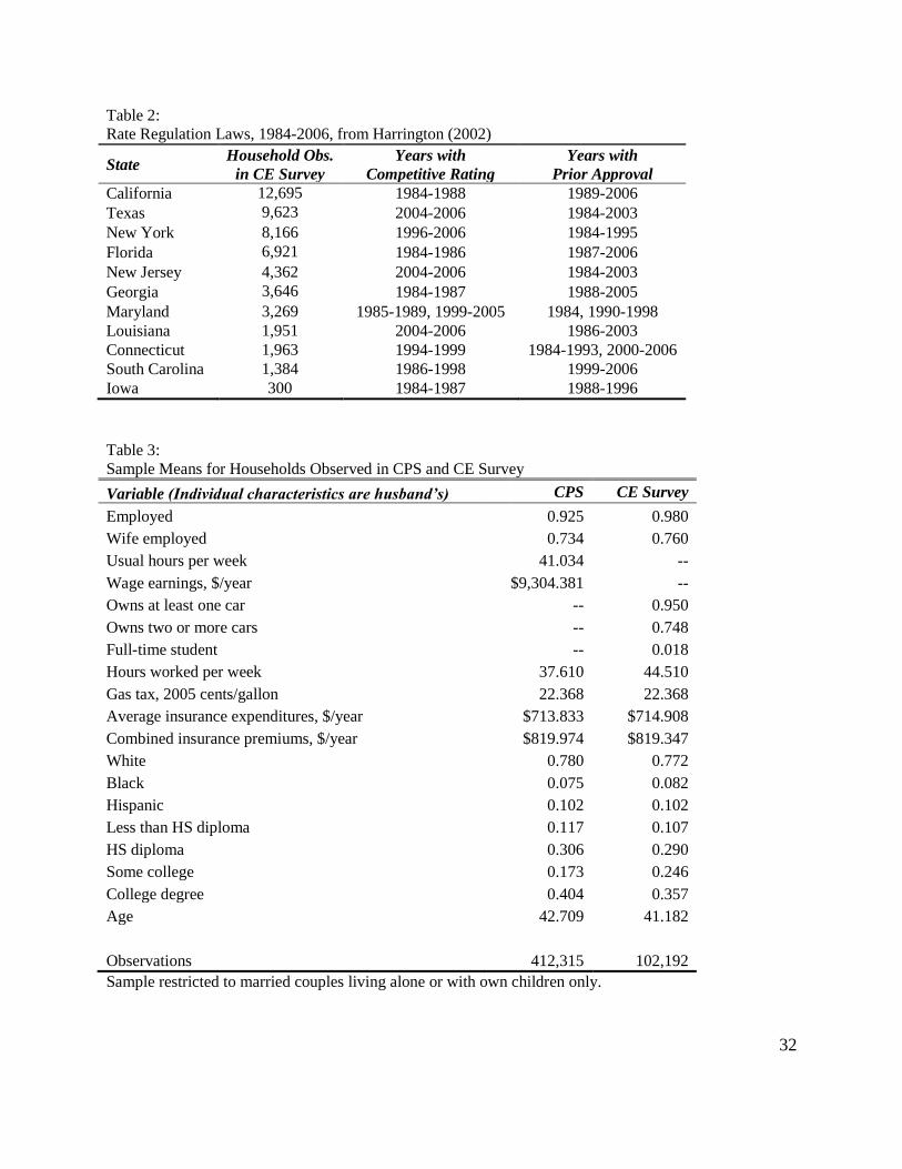
32

Table 2:

Rate Regulation Laws, 1984-2006, from Harrington (2002)

State Household Obs.

in CE Survey

Years with

Competitive Rating

Years with

Prior Approval

California 12,695 1984-1988 1989-2006

Texas 9,623 2004-2006 1984-2003

New York 8,166 1996-2006 1984-1995

Florida 6,921 1984-1986 1987-2006

New Jersey 4,362 2004-2006 1984-2003

Georgia 3,646 1984-1987 1988-2005

Maryland 3,269 1985-1989, 1999-2005 1984, 1990-1998

Louisiana 1,951 2004-2006 1986-2003

Connecticut 1,963 1994-1999 1984-1993, 2000-2006

South Carolina 1,384 1986-1998 1999-2006

Iowa 300 1984-1987 1988-1996

Table 3:

Sample Means for Households Observed in CPS and CE Survey

Sample restricted to married couples living alone or with own children only.

Variable (Individual characteristics are husband’s) CPS CE Survey

Employed 0.925 0.980

Wife employed 0.734 0.760

Usual hours per week 41.034 --

Wage earnings, $/year $9,304.381 --

Owns at least one car -- 0.950

Owns two or more cars -- 0.748

Full-time student -- 0.018

Hours worked per week 37.610 44.510

Gas tax, 2005 cents/gallon 22.368 22.368

Average insurance expenditures, $/year $713.833 $714.908

Combined insurance premiums, $/year $819.974 $819.347

White 0.780 0.772

Black 0.075 0.082

Hispanic 0.102 0.102

Less than HS diploma 0.117 0.107

HS diploma 0.306 0.290

Some college 0.173 0.246

College degree 0.404 0.357

Age 42.709 41.182

Observations 412,315 102,192

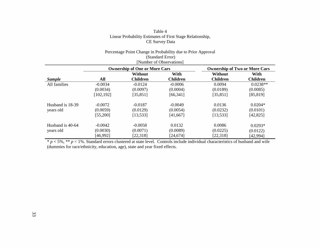
33

Table 4

Linear Probability Estimates of First Stage Relationship,

CE Survey Data

Percentage Point Change in Probability due to Prior Approval

(Standard Error)

[Number of Observations]

Ownership of One or More Cars Ownership of Two or More Cars

Sample

All

Without

Children

With

Children

Without

Children

With

Children

All families -0.0034

(0.0034)

[102,192]

-0.0124

(0.0097)

[35,851]

-0.0006

(0.0004)

[66,341]

0.0094

(0.0189)

[35,851]

0.0238**

(0.0085)

[85,819]

Husband is 18-39

years old

-0.0072

(0.0059)

[55,200]

-0.0187

(0.0129)

[13,533]

-0.0049

(0.0054)

[41,667]

0.0136

(0.0232)

[13,533]

0.0204*

(0.0101)

[42,825]

Husband is 40-64

years old

-0.0042

(0.0030)

[46,992]

-0.0058

(0.0071)

[22,318]

0.0132

(0.0089)

[24,674]

0.0086

(0.0225)

[22,318]

0.0293*

(0.0122)

[42,994]

* p < 5%, ** p < 1%. Standard errors clustered at state level. Controls include individual characteristics of husband and wife

(dummies for race/ethnicity, education, age), state and year fixed effects.

34

Table 5

First-Stage, Reduced-Form, and 2SIV Results from Instrumenting for Two-Car Ownership‘s Effect on

Household Labor Supply with ―Prior Approval‖ Rate Regulation,

among Married Couples with Children

Percentage Point Change in Probability due to Prior Approval

(Standard Error)

[Number of Observations]

1st Stage

(CEX)

Reduced Form (CPS)

Two-Sample IV

Sample consists of households in which:

Husband

Employed

Wife

Employed

Husband

Employed

Wife

Employed

Full sample (i.e. all married couples with

children) 0.024**

0.015** -0.017*

0.617* -0.693

(0.008)

(0.002) (0.007)

(0.243) (0.383)

[85,819] [192,841]

Husband is 18-39 years old 0.020*

0.019** -0.018*

0.922 -0.885

(0.010)

(0.003) (0.007)

(0.481) (0.559)

[42,825] [117,446]

Husband is 40-64 years old 0.029*

0.007* -0.010

0.236 -0.356

(0.012)

(0.003) (0.006)

(0.135) (0.258)

[42,994] [192,841]

Wife is 18-39 years old 0.026*

0.019** -0.017*

0.720* -0.637

(0.012)

(0.003) (0.007)

(0.340) (0.392)

[50,564] [139,364]

Wife is 40-64 years old 0.025*

0.003 -0.010

0.116 -0.391

(0.011)

(0.005) (0.005)

(0.189) (0.276)

[35,255] [53,477]

Husband is older than wife 0.019*

0.014** -0.018**

0.763* -0.936

(0.008)

(0.004) (0.007)

(0.368) (0.541)

[56,899] [130,559]

Wife is at least as old as husband 0.031*

0.013** -0.015

0.409 -0.471

(0.015)

(0.003) (0.009)

(0.215) (0.361)

[28,920] [62,282]

Instrument is indicator for whether ―prior approval‖ rate regulation is in effect in a given state-year. Endogenous

variable is ownership of two or more cars. Sample is restricted to married couples with children.

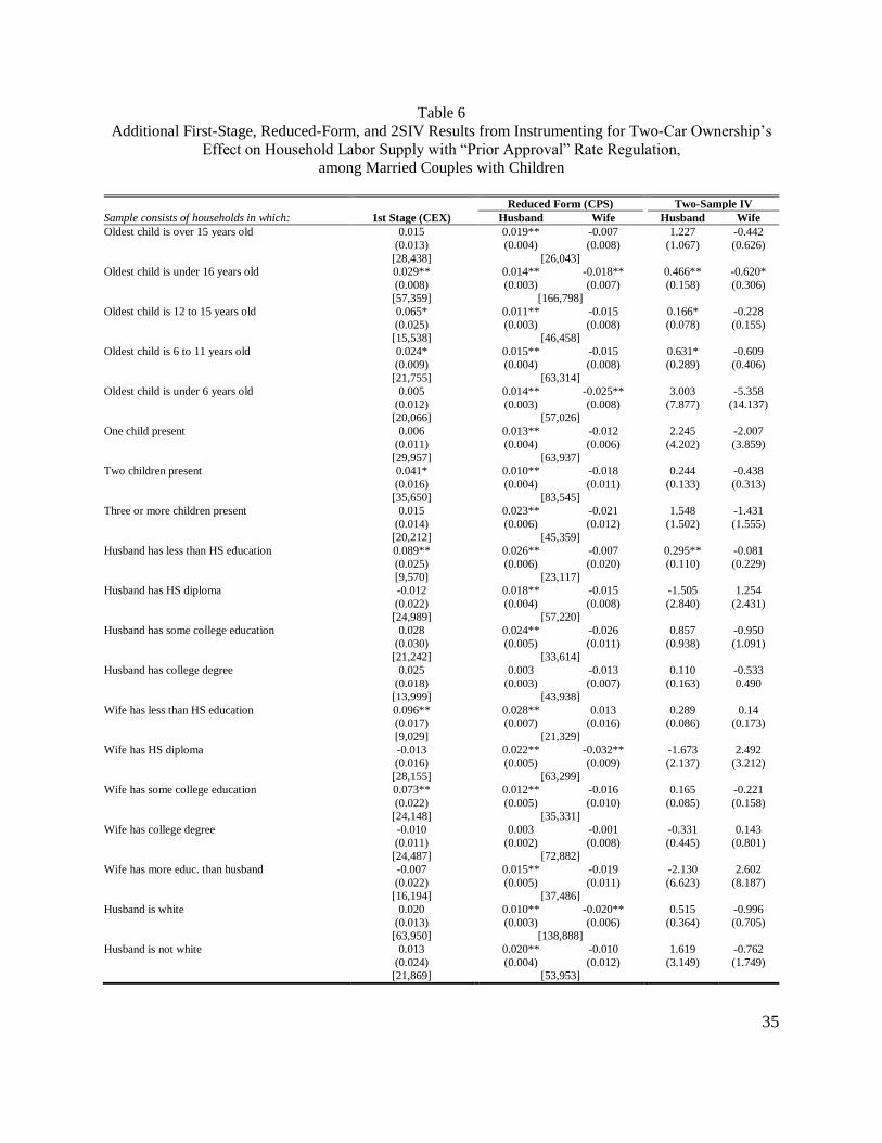
35

Table 6

Additional First-Stage, Reduced-Form, and 2SIV Results from Instrumenting for Two-Car Ownership‘s

Effect on Household Labor Supply with ―Prior Approval‖ Rate Regulation,

among Married Couples with Children

Reduced Form (CPS)

Two-Sample IV

Sample consists of households in which: 1st Stage (CEX)

Husband Wife

Husband Wife

Oldest child is over 15 years old 0.015

0.019** -0.007

1.227 -0.442

(0.013)

(0.004) (0.008)

(1.067) (0.626)

[28,438] [26,043] Oldest child is under 16 years old 0.029**

0.014** -0.018**

0.466** -0.620*

(0.008)

(0.003) (0.007)

(0.158) (0.306) [57,359] [166,798]

Oldest child is 12 to 15 years old 0.065*

0.011** -0.015

0.166* -0.228

(0.025)

(0.003) (0.008)

(0.078) (0.155) [15,538] [46,458]

Oldest child is 6 to 11 years old 0.024*

0.015** -0.015

0.631* -0.609

(0.009)

(0.004) (0.008)

(0.289) (0.406)

[21,755] [63,314]

Oldest child is under 6 years old 0.005

0.014** -0.025**

3.003 -5.358

(0.012)

(0.003) (0.008)

(7.877) (14.137) [20,066] [57,026]

One child present 0.006

0.013** -0.012

2.245 -2.007

(0.011)

(0.004) (0.006)

(4.202) (3.859) [29,957] [63,937]

Two children present 0.041*

0.010** -0.018

0.244 -0.438

(0.016)

(0.004) (0.011)

(0.133) (0.313) [35,650] [83,545]

Three or more children present 0.015

0.023** -0.021

1.548 -1.431

(0.014)

(0.006) (0.012)

(1.502) (1.555) [20,212] [45,359]

Husband has less than HS education 0.089**

0.026** -0.007

0.295** -0.081

(0.025)

(0.006) (0.020)

(0.110) (0.229) [9,570] [23,117]

Husband has HS diploma -0.012

0.018** -0.015

-1.505 1.254

(0.022)

(0.004) (0.008)

(2.840) (2.431) [24,989] [57,220]

Husband has some college education 0.028

0.024** -0.026

0.857 -0.950

(0.030)

(0.005) (0.011)

(0.938) (1.091) [21,242] [33,614]

Husband has college degree 0.025

0.003 -0.013

0.110 -0.533

(0.018)

(0.003) (0.007)

(0.163) 0.490 [13,999] [43,938]

Wife has less than HS education 0.096**

0.028** 0.013

0.289 0.14

(0.017)

(0.007) (0.016)

(0.086) (0.173) [9,029] [21,329]

Wife has HS diploma -0.013

0.022** -0.032**

-1.673 2.492

(0.016)

(0.005) (0.009)

(2.137) (3.212) [28,155] [63,299]

Wife has some college education 0.073**

0.012** -0.016

0.165 -0.221

(0.022)

(0.005) (0.010)

(0.085) (0.158) [24,148] [35,331]

Wife has college degree -0.010

0.003 -0.001

-0.331 0.143

(0.011)

(0.002) (0.008)

(0.445) (0.801) [24,487] [72,882]

Wife has more educ. than husband -0.007

0.015** -0.019

-2.130 2.602

(0.022)

(0.005) (0.011)

(6.623) (8.187) [16,194] [37,486]

Husband is white 0.020

0.010** -0.020**

0.515 -0.996

(0.013)

(0.003) (0.006)

(0.364) (0.705) [63,950] [138,888]

Husband is not white 0.013

0.020** -0.010

1.619 -0.762

(0.024)

(0.004) (0.012)

(3.149) (1.749) [21,869] [53,953]

36

* p < 5%, ** p < 1%. Standard errors clustered at state level. Controls include individual characteristics of husband and wife (dummies for

race/ethnicity, education, age), size of family, state and year fixed effects.

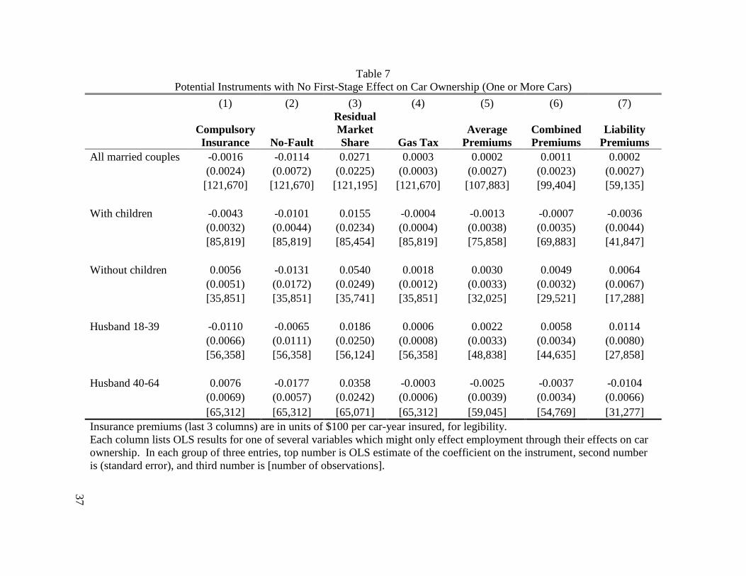
37

Table 7

Potential Instruments with No First-Stage Effect on Car Ownership (One or More Cars)

(1) (2) (3) (4) (5) (6) (7)

Compulsory

Insurance No-Fault

Residual

Market

Share Gas Tax

Average

Premiums

Combined

Premiums

Liability

Premiums

All married couples -0.0016 -0.0114 0.0271 0.0003 0.0002 0.0011 0.0002

(0.0024) (0.0072) (0.0225) (0.0003) (0.0027) (0.0023) (0.0027)

[121,670] [121,670] [121,195] [121,670] [107,883] [99,404] [59,135]

With children -0.0043 -0.0101 0.0155 -0.0004 -0.0013 -0.0007 -0.0036

(0.0032) (0.0044) (0.0234) (0.0004) (0.0038) (0.0035) (0.0044)

[85,819] [85,819] [85,454] [85,819] [75,858] [69,883] [41,847]

Without children 0.0056 -0.0131 0.0540 0.0018 0.0030 0.0049 0.0064

(0.0051) (0.0172) (0.0249) (0.0012) (0.0033) (0.0032) (0.0067)

[35,851] [35,851] [35,741] [35,851] [32,025] [29,521] [17,288]

Husband 18-39 -0.0110 -0.0065 0.0186 0.0006 0.0022 0.0058 0.0114

(0.0066) (0.0111) (0.0250) (0.0008) (0.0033) (0.0034) (0.0080)

[56,358] [56,358] [56,124] [56,358] [48,838] [44,635] [27,858]

Husband 40-64 0.0076 -0.0177 0.0358 -0.0003 -0.0025 -0.0037 -0.0104

(0.0069) (0.0057) (0.0242) (0.0006) (0.0039) (0.0034) (0.0066)

[65,312] [65,312] [65,071] [65,312] [59,045] [54,769] [31,277]

Insurance premiums (last 3 columns) are in units of $100 per car-year insured, for legibility.

Each column lists OLS results for one of several variables which might only effect employment through their effects on car

ownership. In each group of three entries, top number is OLS estimate of the coefficient on the instrument, second number

is (standard error), and third number is [number of observations].

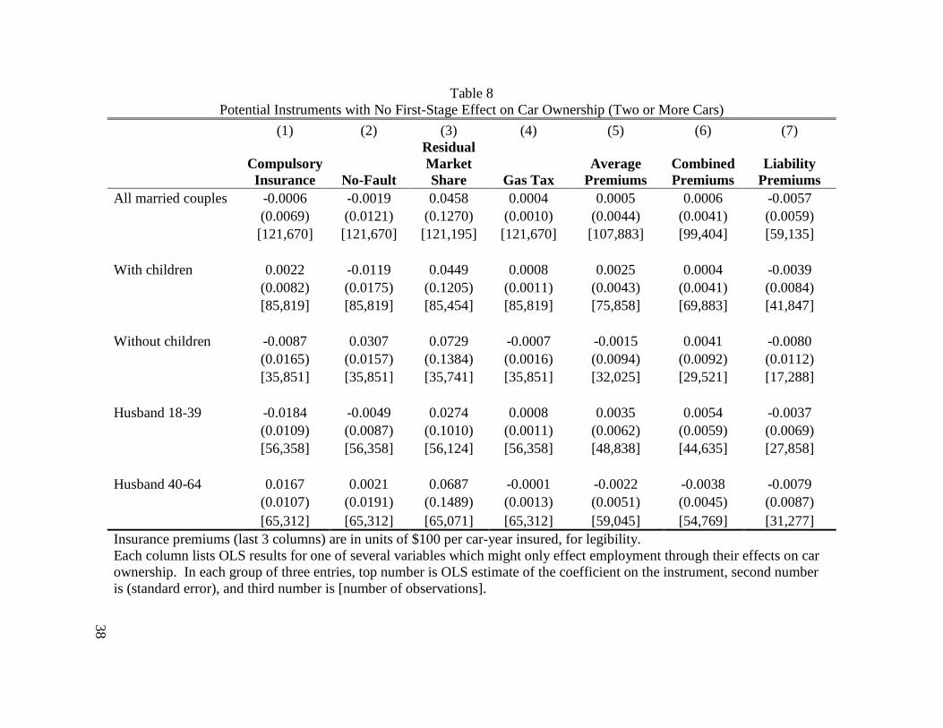
38

Table 8

Potential Instruments with No First-Stage Effect on Car Ownership (Two or More Cars)

(1) (2) (3) (4) (5) (6) (7)

Compulsory

Insurance No-Fault

Residual

Market

Share Gas Tax

Average

Premiums

Combined

Premiums

Liability

Premiums

All married couples -0.0006 -0.0019 0.0458 0.0004 0.0005 0.0006 -0.0057

(0.0069) (0.0121) (0.1270) (0.0010) (0.0044) (0.0041) (0.0059)

[121,670] [121,670] [121,195] [121,670] [107,883] [99,404] [59,135]

With children 0.0022 -0.0119 0.0449 0.0008 0.0025 0.0004 -0.0039

(0.0082) (0.0175) (0.1205) (0.0011) (0.0043) (0.0041) (0.0084)

[85,819] [85,819] [85,454] [85,819] [75,858] [69,883] [41,847]

Without children -0.0087 0.0307 0.0729 -0.0007 -0.0015 0.0041 -0.0080

(0.0165) (0.0157) (0.1384) (0.0016) (0.0094) (0.0092) (0.0112)

[35,851] [35,851] [35,741] [35,851] [32,025] [29,521] [17,288]

Husband 18-39 -0.0184 -0.0049 0.0274 0.0008 0.0035 0.0054 -0.0037

(0.0109) (0.0087) (0.1010) (0.0011) (0.0062) (0.0059) (0.0069)

[56,358] [56,358] [56,124] [56,358] [48,838] [44,635] [27,858]

Husband 40-64 0.0167 0.0021 0.0687 -0.0001 -0.0022 -0.0038 -0.0079

(0.0107) (0.0191) (0.1489) (0.0013) (0.0051) (0.0045) (0.0087)

[65,312] [65,312] [65,071] [65,312] [59,045] [54,769] [31,277]

Insurance premiums (last 3 columns) are in units of $100 per car-year insured, for legibility.

Each column lists OLS results for one of several variables which might only effect employment through their effects on car

ownership. In each group of three entries, top number is OLS estimate of the coefficient on the instrument, second number

is (standard error), and third number is [number of observations].

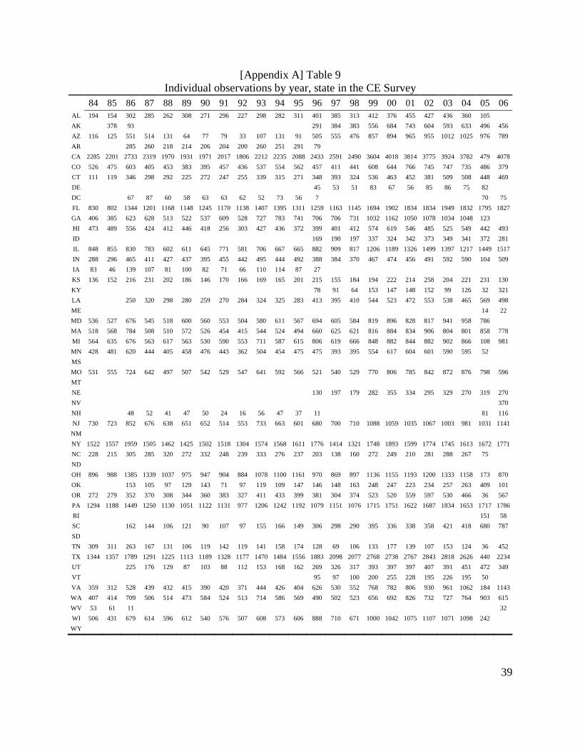
39

[Appendix A] Table 9

Individual observations by year, state in the CE Survey

84 85 86 87 88 89 90 91 92 93 94 95 96 97 98 99 00 01 02 03 04 05 06

AL 194 154 302 285 262 308 271 296 227 298 282 311 401 385 313 412 376 455 427 436 360 105

AK

378 93

291 384 383 556 684 743 604 593 633 496 456

AZ 116 125 551 514 131 64 77 79 33 107 131 91 505 555 476 857 894 965 955 1012 1025 976 789

AR

285 260 218 214 206 204 200 260 251 291 79

CA 2285 2201 2733 2319 1970 1931 1971 2017 1806 2212 2235 2088 2433 2591 2490 3604 4018 3814 3775 3924 3782 479 4078

CO 526 475 603 405 453 383 395 457 436 537 554 562 457 411 441 608 644 766 745 747 735 486 379

CT 111 119 346 298 292 225 272 247 255 339 315 271 348 393 324 536 463 452 381 509 508 448 469

DE

45 53 51 83 67 56 85 86 75 82

DC

67 87 60 58 63 63 62 52 73 56 7

70 75

FL 830 802 1344 1201 1168 1148 1245 1170 1138 1407 1395 1311 1259 1163 1145 1694 1902 1834 1834 1949 1832 1795 1827

GA 406 385 623 628 513 522 537 609 528 727 783 741 706 706 731 1032 1162 1050 1078 1034 1048 123

HI 473 489 556 424 412 446 418 256 303 427 436 372 399 401 412 574 619 546 485 525 549 442 493

ID

169 190 197 337 324 342 373 349 341 372 281

IL 848 855 830 783 602 611 645 771 581 706 667 665 882 909 817 1206 1189 1326 1499 1397 1217 1449 1517

IN 288 296 465 411 427 437 395 455 442 495 444 492 388 384 370 467 474 456 491 592 590 104 509

IA 83 46 139 107 81 100 82 71 66 110 114 87 27

KS 136 152 216 231 202 186 146 170 166 169 165 201 215 155 184 194 222 214 258 204 221 231 130

KY

78 91 64 153 147 148 152 99 126 32 321

LA

250 320 298 280 259 270 284 324 325 283 413 395 410 544 523 472 553 538 465 569 498

ME

14 22

MD 536 527 676 545 518 600 560 553 504 580 611 567 694 605 584 819 896 828 817 941 958 786

MA 518 568 784 508 510 572 526 454 415 544 524 494 660 625 621 816 884 834 906 804 801 858 778

MI 564 635 676 563 617 563 530 590 553 711 587 615 806 619 666 848 882 844 882 902 866 108 981

MN 428 481 620 444 405 458 476 443 362 504 454 475 475 393 395 554 617 604 601 590 595 52

MS

MO 531 555 724 642 497 507 542 529 547 641 592 566 521 540 529 770 806 785 842 872 876 798 596

MT

NE

130 197 179 282 355 334 295 329 270 319 270

NV

370

NH

48 52 41 47 50 24 16 56 47 37 11

81 116

NJ 730 723 852 676 638 651 652 514 553 733 663 601 680 700 710 1088 1059 1035 1067 1003 981 1031 1141

NM

NY 1522 1557 1959 1505 1462 1425 1502 1518 1304 1574 1568 1611 1776 1414 1321 1748 1893 1599 1774 1745 1613 1672 1771

NC 228 215 305 285 320 272 332 248 239 333 276 237 203 138 160 272 249 210 281 288 267 75

ND

OH 896 988 1385 1339 1037 975 947 904 884 1078 1100 1161 970 869 897 1136 1155 1193 1200 1333 1158 173 870

OK

153 105 97 129 143 71 97 119 109 147 146 148 163 248 247 223 234 257 263 409 101

OR 272 279 352 370 308 344 360 383 327 411 433 399 381 304 374 523 520 559 597 530 466 36 567

PA 1294 1188 1449 1250 1130 1051 1122 1131 977 1206 1242 1192 1079 1151 1076 1715 1751 1622 1687 1834 1653 1717 1786

RI

151 58

SC

162 144 106 121 90 107 97 155 166 149 306 298 290 395 336 338 358 421 418 680 787

SD

TN 309 311 263 167 131 106 119 142 119 141 158 174 128 69 106 133 177 139 107 153 124 36 452

TX 1344 1357 1789 1291 1225 1113 1189 1328 1177 1470 1484 1556 1883 2098 2077 2768 2738 2767 2843 2818 2626 440 2234

UT

225 176 129 87 103 88 112 153 168 162 269 326 317 393 397 397 407 391 451 472 349

VT

95 97 100 200 255 228 195 226 195 50

VA 359 312 528 439 432 415 390 420 371 444 426 404 626 530 552 768 782 806 930 961 1062 184 1143

WA 407 414 709 506 514 473 584 524 513 714 586 569 490 502 523 656 692 826 732 727 764 903 615

WV 53 61 11

32

WI 506 431 679 614 596 612 540 576 507 608 573 606 888 710 671 1000 1042 1075 1107 1071 1098 242

WY