The effect of baroclinicity on the wind in the planetary

Quarterly Journal of the Royal Meteorological Society Q. J. R. Meteorol. Soc. 00: 1–16 (2011)

The effect of baroclinicity on the wind in the planetaryboundary layer

R. Floors1∗A. Peña1 and S-E. Gryning1

1 DTU Wind Energy, Technical University of Denmark, Roskilde, Denmark∗Correspondence to: DTU Wind Energy, Risø Campus, Technical University of Denmark, P.O. Box 49, Frederiksborgvej

399, 4000, Roskilde, DenmarkE-mail: [email protected]

The influence of baroclinicity on wind within the planetary boundary layeris investigated using two years of wind lidar measurements collected at asuburban site in northern Germany (Hamburg) and a rural-coastal site inwestern Denmark (Høvsøre). Measurements are made up to a height of950 m. The surface geostrophic wind, the surface gradient wind and thegradient wind are estimated using the pressure and geopotential fields from amesoscale model. At both sites the atmospheric flow was typically baroclinic.The distribution of the geostrophic wind shear was approximately Gaussianwith a mean close to zero and a standard deviation of approximately 3 m s−1

km−1. The geostrophic wind shear had a strong seasonal dependence becauseof temperature differences between land and sea. The mean wind profile inHamburg, observed during an intensive campaign using radio sounding andduring the whole year using the wind lidar, was influenced by baroclinicity.For easterly winds at Høvsøre, the estimated gradient wind decreased rapidlywith height, resulting in a mean low-level jet. The cross-isobaric angle, theboundary-layer height and the empirical constants in the geostrophic drag lawwere found to be dependent on baroclinicity for neutral conditions.

Copyright © 2011 Royal Meteorological Society

Key Words: baroclinicity, Geostrophic Wind, Gradient Wind, Wind Profile, Wind Lidar, Weather Researchand Forecasting

Received . . .

Citation: . . .

1. Introduction

Knowledge of the wind speed in the planetary boundarylayer (PBL) is required for a wide range of applicationssuch as numerical weather prediction (NWP) and airpollution modelling, and is of great importance to the5

wind energy industry. With the emergence of tall windturbines that operate above the surface layer, therehas been an increased interest in the processes thatinfluence winds higher up in the PBL. The logarithmicwind profile and Monin-Obukhov similarity theory10

(MOST) have been succesfully used to describe thewind profile in the surface layer (Holtslag 1984). Above

the PBL, the pressure gradient and Coriolis forces arenearly in equilibrium with each other, and the flowcan be approximated as geostrophic. Baroclinicity is a15

phenomenon that influences the wind profile throughoutthe atmosphere, but its influence on the wind in thePBL has not received much attention. In a baroclinicatmosphere, horizontal temperature gradients, such asthose found along fronts or formed by differential20

heating, cause the geostrophic wind to change with height(geostrophic wind shear). In this paper, we investigate theimpact of the estimated geostrophic wind shear on windspeed observations within the PBL.

Copyright © 2011 Royal Meteorological SocietyPrepared using qjrms4.cls [Version: 2011/05/18 v1.02]

2 R. Floors et al.

The geostrophic wind is an important boundary25

condition in many boundary-layer experiments andmodelling studies. Because the variation in geostrophicwind is relatively small over horizontal distances lessthan tens of kilometers, the geostrophic wind can beassumed to be independent of microscale features of30

the flow and the geostrophic drag law can be applied(Blackadar and Tennekes 1968). This assumption isutilised, for example, in the Wind Atlas Analysis andApplication Program (WAsP) (Troen and Petersen 1989).Zilitinkevich and Esau (2005) showed that part of the35

scatter in the empirical coefficients of the geostrophicdrag law is caused by baroclinicity. Erroneous predictionof geostrophic wind shear can furthermore have a largeimpact on how the wind profile is represented in single-column models, which are used to study the performance40

of NWP models. Baas et al. (2010) varied the geostrophicwind speed and geostrophic wind shear used to force asingle-column model during a low-level jet case study,and found that it had a large impact on the modelled windprofile above 100 m.45

The effect of baroclinicity on the wind profile inthe boundary layer was recognized a long time agoand in the last decades, large-eddy simulation (LES)model output has been used to study the impact ofgeostrophic wind shear on the PBL structure. Brown50

(1996) compared the results from two first-order closureschemes with the model output from LES in neutral andunstable conditions, and found that their performanceswere not degraded by the introduction of geostrophicwind shear. Brown (1999) also investigated the effect of55

a range of geostrophic wind shear intensities on cumulus-cloud parametrization, but found that these had onlya minor impact on entrainment and cloud geometry.Sorbjan (2004) performed more realistic simulations ofthe convective baroclinic boundary layer by taking into60

account the effect of temperature advection and theeffect of baroclinicity on the inversion layer. All ofthese simulations indicated that the first and second-order moments of wind and temperature in the PBL wereinfluenced by baroclinicity.65

There are, however, few experimental studies on theeffect of baroclinicity on flow within the PBL. Firstly,it is difficult to obtain estimates of the thermal windusing near-surface temperature observations, which arestrongly influenced by local conditions (Hess et al. 1981).70

Secondly, temperature profiles derived from radio sondesare often available at just a few locations and launchedtoo infrequently. Finally, many simultaneously varyingparameters influence the wind in the upper part of theboundary layer and, therefore, it is difficult to isolate75

the effect baroclinicity. One of the few studies in whichhorizontal temperature gradients were measured, wasperformed by Lenschow et al. (1980), who investigatedthe turbulent quantities of the baroclinic convective PBL.Hoxit (1974) and Joffre (1982) averaged the results of80

many radiosondes in order to study basic features ofthe baroclinic PBL, and found that the thermal windhad a strong effect on the change of wind directionwith height. Arya and Wyngaard (1975) studied theeffect of baroclinicity on the geostrophic drag law, but85

experimental verification of their model was difficult. Thesmall number of experimental studies shows that moreaccurate observations of the baroclinic PBL are valuable.

In this study, we are able to advance understanding ofthe effects of baroclinicity on winds within the PBL by90

utilising two recent developments. Firstly, the accuracyand range of wind lidars has recently been improved, andthe continuous measurement of wind speed profiles up toheights of around 1000 m is now possible (Floors et al.2013). Secondly, more detailed knowledge of horizontal95

pressure and temperature gradients can nowadays beobtained from mesoscale model output. Here we use theAdvanced Research Weather Research and Forecasting(WRF-ARW) model version 3.4 (hereafter the WRFmodel), a mesoscale model developed by the National100

Center of Atmospheric Research (NCAR) that uses state-of-the-art numerical schemes (Skamarock et al. 2008).The WRF model can accurately describe wind andtemperature fields up to scales of around a few kilometres(Hu et al. 2010; Xie et al. 2012; Gryning et al. 2013b).105

Here, we use data from a wind lidar operatingfor 1 year at a coastal site in Denmark and afterthat for 1 year at a suburban site in Hamburg. Atboth sites a meteorological mast or television tower isavailable to provide mean wind speeds and turbulence110

statistics. In addition, radiosondes, launched during anintensive campaign, are used. Combining the novelwind lidar measurements with the large-scale parametersestimated from the mesoscale model output can give acomprehensive overview of the role of baroclinicity on115

winds in the PBL.The study is presented as follows. First, an overview

of the theory describing the flow in the baroclinic PBLis given in (Section 2). In Section 3, descriptions of thestudy sites and methods for data processing, estimation120

of geostrophic wind based on mesoscale model outputand filtering are presented. In Section 4.1 a comparisonof wind speeds obtained from the different instrumentsis given. The impact of baroclinicity on the wind speedclimatologies of both sites, is investigated in Section 4.2.125

Next, a study of the influence of baroclinicity on the windprofile in the PBL using the wind profile measurementsfrom the wind lidar and the radiosondes is presented(Section 4.3). The effect of baroclinicity on the windveer in the PBL, and on the constants in the geostrophic130

drag law, is discussed in Section 4.4. Finally, we presentconcluding remarks in Section 5.

2. Theory

Using Reynolds decomposition, and in a Cartesiancoordinate system, the wind can be decomposed into the135

mean velocities U , V and W and their correspondingturbulent parts u�, v� and w�. In a left-handed geographiccoordinate system, x corresponds to the east-westdirection, y to the north-south direction and z to theheight above the surface. Assuming a horizontally140

homogeneous, stationary flow where the mean verticalvelocity is zero, the equations of motion in the PBL aregiven by a balance between the friction force, the pressuregradient force and the Coriolis force,

∂∂ z

u�w� = f (V −Vg), (1)

145∂∂ z

v�w� = f (Ug −U), (2)

Copyright © 2011 Royal Meteorological Society Q. J. R. Meteorol. Soc. 00: 1–16 (2011)Prepared using qjrms4.cls

The effect of baroclinicity on the wind in the planetary boundary layer 3

where f is the Coriolis parameter and Ug and Vg are thegeostrophic wind speed components,

Ug =−1/( f ρ0)∂P/∂y, (3)

Vg = 1/( f ρ0)∂P/∂x, (4)

where ρ0 is the background air density and P is theatmospheric pressure. It is convenient to analyze the wind150

profile in a coordinate system that is aligned with thewind direction at the surface; we use a left-handedcoordinate system. From now on, we use the capitalletters U and V to denote the components of windspeed in the directions parallel with the axes of the155

geographic coordinate system and the letters u and v forthe components that are aligned and perpendicular withrespect to the surface-layer wind, respectively.

The geostrophic flow is parallel to the isobars, withthe low pressure to the left on the Northern hemisphere.160

Because there is little friction above the PBL height, onecan assume the flow can be described as an equilibriumbetween the pressure gradient and the Coriolis force. Ifthe pressure gradient is measured at the surface or if it isreduced to the pressure at mean sea level, it is denoted165

as the surface geostrophic wind with components Ug0and Vg0. In barotropic conditions, the geostrophic windat any height is equal to the surface geostrophic wind, i.e.Ug = Ug0.

When horizontal temperature gradients are present,170

the atmosphere becomes baroclinic and Ug changes withheight. The vector difference between the geostrophicwind at two heights is referred to as the thermal wind;its components, UT and VT , can be expressed in termsof the horizontal gradients of the geopotential difference175

between two layers (Holton and Hakim 2004),

UT =− 1f

∂ (Φz −Φ0)

∂y, (5)

VT =1f

∂ (Φz −Φ0)

∂x, (6)

where Φz and Φ0 are the geopotentials at the top and atthe bottom of the layer, respectively. The thermal windvector is parallel to the isotherms with the cold air to the180

left.When the pressure gradient is estimated over some

finite area, one has to assume that the pressure fieldvaries linearly with x and y. However, when there is acyclonic or anti-cyclonic flow, the second derivatives of185

the pressure field are not zero, i.e. the isobars cannotbe considered to be straight. The radius of curvature Rof the isobars is positive around a low pressure systemand negative around a high pressure system. When theisobars are curved, the centrifugal acceleration becomes190

important and the atmospheric forcing can be estimatedby assuming it is well described by the gradient windGgr. The flow is then described by a balance between thecentrifugal force, the Coriolis force and the pressure force(Holton and Hakim 2004),195

G2gr

R+ f Ggr − f G = 0. (7)

Dividing Eq. 7 by f G, and solving for Ggr/G, the resultis one physically meaningful solution,

Ggr

G=

−1+�

1+4G/( f R)2G/ f R

. (8)

Generally, the difference between the gradient andgeostrophic wind is less than 10-20% at midlatitudes(Holton and Hakim 2004). Furthermore, it follows from200

Eq. (7) that,

Ggr =G

1+Rogr, (9)

where the gradient Rossby number is given by Rogr =Ggr/ f R. The assumption ∂Ggr/∂ z ∼ ∂G/∂ z can beevaluated by taking the vertical derivative of Eq. (9)(Section 3.3). Assuming ∂Ggr/∂ z ∼ ∂G/∂ z and because205

the direction of the gradient and geostrophic wind vectorsare the same, the gradient wind at a certain height can beestimated by adding the thermal wind components to thegradient wind near the surface,

Ugr =Ugr0 +UT , (10)

210

Vgr =Vgr0 +VT . (11)

Kristensen and Jensen (1999) assumed that the pressurefield in a certain area can be described by,

p(x,y) = p0 + px + py +0.5(p2xx +2pxy + p2

yy), (12)

where p0 is a reference pressure and the subscript denotesfirst (one letter) and second derivatives (two letters) withrespect to the differentiated dimension. From this field the215

curvature can be estimated as,

R =(p2

x + p2y)

3/2

pyy p2x −2pxy px py + pxx p2

y. (13)

In order to introduce the terminology used in previouswork on baroclinic effects in the PBL (Hoxit 1974) andadopted in this paper, Figures 1a and 1b show a vector220

plot and the wind speed profile for a situation withpositive geostrophic wind shear and veer. The figure isvalid for a situation when R → ∞, but for a finite Rthe surface geostrophic wind and the geostrophic windcan be substituted with the surface gradient wind and225

the gradient wind, respectively. β is defined as the anglemeasured clockwise between Ug0 and UT at the PBLheight h. When 0◦ < β < 180◦, warm air advection occursand when 180◦ < β < 360◦, cold air advection occurs.U0 is defined as the surface-layer wind, and α is defined230

as the angle measured clockwise between U0 and Ug0.α ≈ 20◦ in a neutral PBL at mid-latitudes due to the effectof friction near the surface (Hess and Garratt 2002a). φis defined as the angle between U0 and Ug at the PBLheight.235

Equations (1) and (2), in a coordinate system alignedwith the surface-layer wind, are the starting point forthe derivation of the geostrophic drag law, which can beobtained by using the scaling relations for the inner andouter layer, u/u∗ = Fi(z/z0) and (u− ug)/u∗ = Fo(z/h),240

respectively, where u∗ is the friction velocity, z0 is thesurface roughness length and Fi and Fo are functions


4 R. Floors et al.

Ug0

U0

UgUT

α

φ

β

Hei

ght

Wind speedU0 G0

G

a) b)

h

Figure 1. Behaviour of the wind vector looking upwards through thePBL when R → ∞ in baroclinic conditions (left panel), and the windprofile under conditions of positive geostrophic wind shear (right panel).U0, Ug0, Ug and UT denote the surface-layer wind, surface-geostropicwind, geostrophic wind at PBL height h and thermal wind between thesurface and h, respectively. U0, G0 and G denote the magnitude of thesevectors. α , β and φ denote the angle between U0 and Ug0, between Ug0and UT and between U0 and Ug, respectively.

relating to the inner and outer layers, respectively.Blackadar and Tennekes (1968) used the asymptoticbehaviour of the vertical derivatives of the velocity245

profiles in the inner and outer layer to show that in neutral,barotropic conditions,

ug

u∗=

1κ

�ln� h

z0−A

��, (14)

vg

u∗=

Bκ, (15)

where κ is the von Kármán constant (≈ 0.4) and h ≡u∗/ f . Combining the two components ug and vg results in250

a relationship between the magnitude of the geostrophicwind G =

�u2

g + v2g, φ = arctan(vg/ug), u∗ and the two

integration constants A and B, which can be written as,

A = ln�

u∗f z0

�− (κG/u∗)cosφ , (16)

B =±κG/u∗ sinφ , (17)

where, on the right hand side of Eq. (17), a plus and a255

minus sign are applied for the Northern and SouthernHemisphere, respectively. It should be noted that therehas been some confusion in literature over the form ofthe geostrophic drag law, for example, in some workthe constants A and B are reversed whilst Hess and260

Garratt (2002a) showed positive cross-isobaric angles,contradicting what was stated in their Eq. (2).

Even in neutral and barotropic conditions, the scatterin the constants A and B is very large, when determinedfrom experimental data. This is attributed to violations of265

the assumptions in Eqs. (1) and (2). Eqs. (16) and (17),however, are still used to estimate the geostrophic windin a simple way based on variables that can be observednear the surface (Troen and Petersen 1989). An extensiveoverview of the numerous field experiments aimed at270

determining A and B for the neutral, barotropic PBL isgiven in Hess and Garratt (2002a,b).

Zilitinkevich (1975) and Zilitinkevich and Esau (2005)showed that in non-neutral, non-barotropic conditions theinternal stability parameter, baroclinicity and the free-275

flow stability all influence A and B. When these effectswere taken into account in a new formulation of A and B,LES simulations agreed better with the geostrophic draglaw (Zilitinkevich and Esau 2005).

3. Methodology280

For this study, a new long-range, pulsed wind lidar(WLS70) from the company Leosphere was used.Technical details of this instrument can be found inCariou and Boquet (2013). The wind lidar was operatedat two sites equipped with tall meteorological masts.285

First, we will introduce the geographical and micro-meteorological characteristics of the rural-coastal site inDenmark and the suburban site in Hamburg (Section3.1). The data processing is presented in Section 3.2 andin Section 3.3 we present the method used to estimate290

atmospheric forcing from the mesoscale model output.Finally, the filtering of the data sets is presented in Section3.4.

3.1. Sites

3.1.1. Høvsøre295

The first experimental site is the National Test Station ofWind Turbines at Høvsøre in the west of Denmark (56◦26’ 00” N 8◦ 09’ 00” E, figure 2). From 23 April 2010to 29 March 2011, the wind lidar was operating at thissite. The wind lidar was placed 10 m west of a 116.5300

m high meteorological mast. The terrain around the siteconsists of grasslands and the North Sea is located ≈ 1.7km to the west. Wind speed is measured with Risø cupanemometers on booms mounted on the southern side ofthe mast at heights of 10, 60, and 100 m. Wind direction305

is measured at 100 m.Turbulent fluxes are measured with a METEK

Scientific USA-1 sonic anemometer at 10 m on a boomdirected to the north. With westerly winds, the flow atthe site is influenced by the internal boundary layer that310

forms after the smooth-to-rough surface change at theshoreline of Denmark (Floors et al. 2011). For northerlyflow, there is influence from the wakes of the mast and thewind turbines and, therefore, only data from the easterlysector were used. The wind direction for the easterly315

sector ranged between 30◦–140◦. It is assumed that u∗and w�θ � at 10 m are representative of the surface-layervalues u∗0 and w�θ �0, respectively. In Floors et al. (2013)it was shown that the blending height for the easterlysector is ≈ 10 m. The wind profiles from the lidar were320

rotated such that the wind direction at 100 m was the sameas measured by the wind vane. An exponent idealizedprofile method was used to obtain the PBL height froma ceilometer (CL31) from the company Väisälä operatingat the site (Steyn et al. 1999; Hannesdóttir 2013).325

3.1.2. Hamburg

The wind lidar was running at the Hamburg site from4 April 2011 to 24 March 2012. There were problemswith the cooling system from the 13th of June and it wastherefore temporarily replaced with a similar device. On330



the 25th of November, the original device was reinstalledand ran without any problems until the 23rd of March2012. The wind lidar was installed on a grass field, 170m to the north-east of a 300 m high television towerand 8 km south-east of downtown Hamburg (53◦ 31’335

11,7” N, 10◦ 06’ 18,5” E, Figure 2). The television towerhas booms mounted on the southern side, where thewind speed, wind direction and turbulence parameterswere measured with METEK Scientific USA-1 sonicanemometers at 50, 110, 175 and 250 m. The wind lidar340

profiles were rotated such that the wind direction at 250m agreed with the wind direction measured by the sonicanemometer at 250 m. Furthermore, a Väisälä ceilometer(CL51) measured atmospheric backscatter profiles, fromwhich h was derived using the algorithm described in345

Münkel et al. (2011).The buildings around the television tower are generally

less than 10 m high and, in an urban environment,the blending height can be estimated as approximately1.5 to 5 times the mean obstacle height (Rotach350

et al. 2005; Batchvarova and Gryning 2005). Therefore,measurements taken at 50 meters height were assumedto equate to surface-layer measurements. For winddirections between 130◦–320◦, the upstream area is theheavily build-up area of the city center of Hamburg, and355

for wind directions between 40◦–130◦, the upstream areais a residential area with a combination of fields, trees andbuildings.

In addition to the tower and wind lidar measurements,two intensive measurement campaigns were performed360

in Hamburg during two 5-day periods in 2011. Thefirst campaign began at 0800 UTC, 15 June 2011 andended at 0800 UTC, 20 June 2011. During this period,60 radiosondes were released, i.e. approximately onesounding every two hours. Two radiosondes did not reach365

an altitude of 5 km and were therefore not used. A secondintensive campaign was performed from 0800 UTC, 4October 2011 until 0700 UTC, 9 October 2011. Alsoduring this period radiosondes were released every twohours, except for the last day when a sounding was370

released every hour. A total of 74 radiosondes werereleased, all of which reached an altitude of 5 km. Themeasurements from the radiosondes were cut into 50-mintervals to compare them with the wind lidar and towerdata. For example, the mean wind speed at 250 m was375

computed by averaging all samples taken between 225and 275 m.

3.2. Data processing

The wind lidar measured the wind speed and the winddirection every 50 m from 100 m up to a maximum of 2380

km, depending on the aerosol content of the atmosphere.The radial wind speed was retrieved at four azimuthalpositions that were separated by 90◦, and the inclinationangle of the beam relative to the zenith was 15◦. Fromthe four radial wind speeds, the three dimensional wind385

vector was constructed assuming horizontal homogeneityof the wind field. One 360◦ full scan (rotation) wasperformed every 30 s. The resulting time series were thenaveraged over a period of 10 minutes.

The 20 Hz signal of the sonic anemometers was390

retrieved and processed with the ECPACK software (VanDijk et al. 2004). Spikes in the raw data signal were

��

��

��

��

��

��

��

��

��

��

��

��

��

��

��

��

��

��

��

��

��

��

Figure 2. Map of the North Sea area. The black squares indicate theareas in which the pressure and geopotential gradients were derived.

removed with the despiking algorithm of Højstrup (1993).When using the eddy-covariance method, it is commonto perform a coordinate rotation to align the mean wind395

vector with the mean stress vector. Here, the planar-fit method was used (Wilczak et al. 2001), where aglobal rotation matrix is calculated based on the meanwind vectors of all 10-minute runs from one month.The resulting tilt angles were then used to rotate all 10-400

minute runs in the direction of the mean streamlinesand an additional rotation was performed such that themean transverse wind component was zero. After linearlydetrending the timeseries, the along-wind (u�w�) andtransversal (v�w�) kinematic stresses can be obtained.405

Similarly, the kinematic heat flux w�θ � can be obtainedusing fluctuations in the potential temperature θ . Across-wind correction was applied for the kinematic heatflux (Schotanus et al. 1983). The friction velocity u∗was calculated as u∗ = (u�w�2 + v�w�2)1/4. The Obukhov410

length L was then estimated as,

L =− u∗03

κ(g/T0)(w�θ �v)0

. (18)

where g is the gravitational acceleration and T0 is thereference temperature, i.e. the temperature measured at2 m at Høvsøre and at 50 m in Hamburg.

3.3. Estimation of the atmospheric forcing415

Many authors have used surface pressure to estimategeostrophic winds, but the effects of thermal wind haveseldom been taken into account (Kristensen and Jensen1999; Baas et al. 2009; Larsén and Mann 2009). Whenbaroclinicity has been taken into account, geostrophic420

wind shear has often been estimated from the gradientof the measured wind speed at or near the top of thePBL (Joffre 1982; Garratt 1985). However, in unstableconditions, the strongest wind shear is present in theentrainment zone, so the measured wind shear near425

the top of the PBL height does not correspond togeostrophic wind shear. Furthermore, the PBL heightitself is inherently uncertain (Seibert et al. 2000).


6 R. Floors et al.

Here, we therefore used the WRF model to estimatethe large-scale winds and the PBL height. The following430

physical parametrization schemes are used:

• Yonsei University PBL scheme (Hong et al. 2006)• MOST based surface-layer scheme (Chen and

Dudhia 2001)• NOAH land-surface scheme (Chen and Dudhia435

2001)• Thompson microphysics scheme (Thompson

et al. 2004)• RRTM longwave radiation (Mlawer et al. 1997)• Dudhia shortwave radiation (Dudhia 1989)440

A coding error in the YSU scheme, that gave too muchmixing for stable conditions in previous versions ofWRF, was removed. The model was run from April 2010until April 2011 for Høvsøre and for April 2011 untilApril 2012 for Hamburg in analysis mode, viz. it was445

started every 10 days at 00 UTC for a period of 264hours. There were two model domains that used two-way nesting and had a horizontal resolution of 18 and 6km. There were 41 levels in the vertical and 10 of thosewere located below 1000 m. After removing the first 24450

hours of spin-up time, 10-minute instantaneous modeloutput from the innermost domain was used. The outerand inner model domains had a time step of 120 and 40s, respectively. The boundary and initial conditions camefrom the NCEP FNL analysis and from the NCEP real-455

time global sea-surface temperature analysis. Nudgingtowards the atmospheric analysis data of the specifichumidity, the potential temperature and U and V , wasapplied in the outermost domain above the 10th modellevel (which corresponds to a height of ∼ 1400 m) and460

only outside the PBL.The described set-up was chosen based on several

sensitivity studies; a one month period in autumn2010 was modelled using two vertical resolutions, tworoughness descriptions, two analysis forcings and two465

PBL schemes. These different set-up choices had animpact on the representation of the wind profile, butnone of them simulated wind speeds significantly betterwhen compared to observations (Floors et al. 2013).Because of the rather long simulation period, it was470

finally decided that the relatively fast first-order YSUPBL scheme and the relatively lower vertical resolutionwould be used. The FNL analyses were chosen basedon its real-time availability, which allowed starting thesimulations immediatly after the wind lidar data became475

available. Nudging of simulations was shown to improvethe representation of the wind speed Weibull-distributionparameters at Høvsøre (Gryning et al. 2013a).

The surface geostrophic wind can be estimated usingEqs. (3) and (4). The mean sea level pressure gradient480

can be readily obtained from the model output, by usingsimple linear regression between the north-south andeast-west grid distances and the mean sea-level pressurefield. The thermal wind can be estimated using Eqs. (5)and (6), with the gradients obtained in a similar fashion485

as those from the pressure field, by performing simplelinear regression between the north-south and east-westgrid distance and the difference between the geopotentialat a specified model level and the surface. ρ0 and f in Eqs.(3), (4), (5) and (6) were obtained from the nearest model490

grid point.

The gradients of geopotential and pressure wereestimated from the model output with squares centred onthe two sites (see Figure 2). The size of these squareswere chosen such that they were sufficiently large to495

determine the radius of curvature of typical mid-latitudeatmospheric systems (∼ 1000 km), but so small that thederived gradients actually represented geostrophic flowat the point of interest. Gradients were calculated for anumber of square grids between 36–360 km, and a value500

of 300 km was chosen based on good agreement betweenthe estimated geostrophic wind and the measurements at950 m.

When the isobars are curved within the square grids,Eq. (7) describes the flow in these squares better than Eqs.505

(3) and (4). Therefore, the obtained surface geostrophicwind is mulitplied by the ratio between the gradientand the geostrophic wind (Eq. (8)). To use Eq. (8),the mean R for the square grids has to be known. Thealgorithm described in Shary (1995) was used to estimate510

all derivatives in Eq. (13) for a set of 3 by 3 grid points.A curvature was then computed for all grid points andspatially averaged over the 300 km squares surroundingthe site.

Our estimation of the gradient wind does not515

include the effect of local accelerations, decelerationsor advection, but these effects will be present in theobservations. If we use a sufficiently large number ofobservations, we assume that most of these effects willcancel out because the long-term mean acceleration or520

advection is negligible.

3.4. Filtering

Data filtering was performed using eight criteria, whichare described below, and the resulting data sets aresummarized in Table 1. In section 4.2, a data set525

that consists of only the WRF model output (‘W’) isused, because climatological features of baroclinicity arediscussed and we included as much data as possible.Therefore, only the following filtering was used:

1. All 10-minute data from the WRF simulations for530

the full period when the lidar was operating at therespective sites.

In section 4.3, the mean wind profiles require thefollowing filtering:

2. 10-minute means were included when all individ-535

ual wind lidar scans in that 10-minute period hada carrier-to-noise ratio CNR larger than −35 dB,and a mean CNR larger than −22 dB. The thresh-old of −22 dB was chosen based on agreementchecks between the lidar and the cup anemometer540

at 100 m. The height where the CNR is largerthan −22 dB is also a good proxy for the meanPBL height (Peña et al. 2013b; Floors et al. 2013).Profiles where the lidar wind speed magnitudeincreased or decreased more than 5 m s−1 per 50545

m were removed as spiky profiles.3. Wind profiles up to 950 m height were selected

where the surface-layer fluxes, the wind speedsfrom the cup anemometers at all heights and thosefrom the wind lidar in the range 100–950 m were550

concurrently available.



4. To prevent strong effects from the wake of thetower, data from the northerly sector ranging from320◦–40◦ were removed in Hamburg. At Høvsøre,only data from the easterly sector were used (30◦–555

140◦).5. To ensure that the wind speed at 950 m

approximately corresponds to geostrophic windspeed, we include only the profiles where thesimulated PBL height from the WRF model is560

lower than 1000 m.6. To exclude unsteady, weak-wind or sea-breeze

conditions, the data where Ggr < 5 m s−1 at 966m (the tenth model level; see section 3.3) wereexcluded. In conditions with Ggr > 5 m s−1, it565

is unlikely that a sea-breeze circulation develops(Tijm et al. 1999).

The data set produced by merging the data from theWRF model, the wind lidar and the mast and performingthe filtering described in the items 1–6 is referred to as570

‘WML’.Finally, in Section 4.4 we present an estimation

of the geostrophic drag law constants in the neutral,baroclinic PBL. We aim to determine A and B fromthe observations and show their dependency on the575

baroclinicity parameter β . However, the coefficients Aand B are dependent on other variables and it is difficultto isolate these dependencies in experimental data. Toclearly discriminate the effect of baroclinicity, A and Bshould ideally be determined from measured variables580

only, because the model output is inherently less accurate.u∗ in Eqs. (16) and (17) is measured at both sites withsonic anemometers, while we assume that the wind speedmeasured by the wind lidar at the PBL height is equalto the geostrophic wind, i.e. Uh = Ug. Then, G and585

φ are estimated from the measured wind lidar profiles.The observed PBL height from the ceilometer is used toestimate the height where the wind vector measured bythe wind lidar is equal to the geostrophic wind vector.The disadvantage of using the PBL height derived from590

the ceilometer is that the amount of profiles available foranalysis is reduced, since it was not always possible toget a reliable estimate for example due to the presence ofclouds (Hannesdóttir 2013).

7. Only profiles where the PBL height could be595

determined from the ceilometers were used.

Finally, z0 can be easily obtained from the measure-ments in the surface layer. The roughness length for theeasterly sector at Høvsøre was determined by applyingthe logarithmic wind profile to the 10-m mean data where600

|L| > 1000 m and inserting the measured u∗ and windspeed at 10 m, which gave z0 ≈ 0.03 m. The roughnesslength for both sectors in Hamburg was computed in asimilar manner, but using the data at 50 m. This results inz0 ≈ 0.52 m for the built-up sector and z0 ≈ 0.39 m for605

the rural sector.The effect of atmospheric stability is known to cause

large scatter in the determination of the coefficients(Zilitinkevich 1975), as well as the Brunt-Väisäläfrequency (Zilitinkevich and Esau 2002). Unfortunately,610

measurements of the Brunt-Väisälä frequency were notavailable, but stability was observed by means of L andso we make use of neutrally stratified data only:

Table 1. Number of profiles N and the percentage of all the 10-minintervals available after applying the filtering (see correspondent textin Section 3.4).

Høvsøre HamburgData set (filter) N Perc. N Perc.W (1) 48816 100 51114 100WML (1–6) 528 1.1 2753 5.4WMLC (1–8) 52 0.11 563 1.1WMR (1,4,6) - - 112 0.22

8. It was assumed that the PBL was neutral when|L| > 1000 m, and only those profiles were615

selected.

The data set obtained by merging data from the WRFmodel, the wind lidar, the mast and the ceilometer andapplying the filtering from items 1–8 is abbreviatedas ‘WMLC’. Finally, a data set from the radio sondes620

(‘WMR’) is obtained by applying the filtering of items1,4 and 6.

4. Results

4.1. Comparison of the instruments

To evaluate the accuracy of the wind speeds obtained625

from the mast, wind lidar and radiosondes, data fromthe various sources at both sites were compared witheach other. The number of 10-min averaged profilesavailable for analysis is given in Table 1. At Høvsøre, theagreement between the wind speed measured by the cup630

Uc and that measured by the wind lidar Ul at 100 m wasvery high, with a squared Pearson correlation coefficientr2 = (cov(Uc,Ul)/σUcσUl )

2 = 0.97 and a mean biasb = 1/N ∑n

i=1(Uli −Uci) = −0.38 m s−1 (−4%). Furtherinformation on the agreement between wind speed and635

wind direction obtained from the mast and the wind lidarcan be found in Peña et al. (2013a).

In Hamburg, the mean wind speed was measuredwith sonic anemometers, and because the televisiontower is rather bulky, it distorts the flow around the640

instrumentation. In addition, the television tower and thewind lidar were located 170 m away from each other,which due to spatial differences increases the scatterbetween the measured wind speeds of both instruments.Still, the combined time series of the two different wind645

lidars and the sonic anemometer at the tower showedgood agreement for the wind speeds at a height of 250m, with r2 = 0.92 and b =−0.22 m s−1 (−2.1 %).

Despite the fact that data from the radiosondes is notavailable in the 10-min means produced by the sonic650

anemometer, the wind speeds obtained from the 112radiosondes agreed fairly well with the mast data at 250m, r2 = 0.84 and b =−0.18 m s−1 (−1.8 %). To evaluatethe accuracy of the wind speed as measured by the windlidar at high altitudes, the wind speeds were compared655

to those measured by the radiosondes at 950 m, but dueto the filtering criteria the number of comparable profileswas limited to 20. At this height the agreement was alsogood, r2 = 0.79 and b =−0.21 m s−1 (−1.3 %).


8 R. Floors et al.

4.2. A climatology of baroclinicity660

In this section, we study the estimates of the atmosphericforcing derived from the WRF simulations. Thedifferences between the estimated surface gradient andsurface geostrophic wind were small, on average atHøvsøre for a whole year Ggr0/G0 ≈ 0.98 with a standard665

deviation of 0.05. In Eq. 10 and 11, we used theassumption that the gradient wind shear is approximatelyequal to the geostrophic wind shear. This can be justifiedby taking the vertical derivative of Eq. (9),

∂Ggr

∂ z=

∂G∂ z

11+Rogr

− G(1+Rogr)2

∂Rogr

∂ z, (19)

and showing that the first term on the right hand side670

is much larger than the second term on the right handside even for relatively large values of Rogr. In thatcase, ∂Ggr/∂ z ≈ ∂G/∂ z. Equation (19) was evaluatedfor 18 August 2010, when a low-pressure system passedDenmark and there was a relatively large curvature675

of the isobars and therefore Rogr was relatively large,Rogr0 ≈ 0.01. There was ∼ 5% difference between themagnitude of the surface gradient wind and the surfacegeostrophic wind. ∂G/∂ z ≈ UT/Δz and ∂Rogr/∂ z ≈ΔRogr/Δz were estimated between the first and tenth680

model level, correspending to heights of 14 and 966 m,respectively. Rogr at 14 m was estimated using the surfacegeostrophic wind and the curvature at that height, whileRogr at 966 m was estimated using the curvature and theWRF model wind speed at that height, assuming that685

in the WRF model U ≈ Ugr. On 18 August 2010, thefirst term on the right hand side of Eq. 19 was nearlytwo orders of magnitude larger than the second term onthe right hand side. Using Rogr and G from either 14 or966 m did not change this result. Therefore, ∂Ggr/∂ z ≈690

∂G/∂ z and we can use Eqs. (10) and (11) to estimatethe gradient wind at any height from the model output.Because the geostrophic wind shear and the gradientwind shear are approximately the same, from now on weuse ‘geostrophic wind shear’ to express both ∂G/∂ z and695

∂Ggr/∂ z.Quantitative descriptions of geostrophic wind shear

are rare. The WRF simulated thermal wind distributionat a specific height are therefore interesting, as theycan illustrate the effect of the thermal wind on the700

wind speed. A histogram of the derived thermal windspeed components in the west-east (UT ) and north-south (VT ) directions is shown for the tenth model level,corresponding to a height of 966 m for Høvsøre and 976m for Hamburg (Figure 3). Because of the filtering of705

the wind lidar profiles, two data sets are studied here:W and WML. The frequency of occurrence in each binis normalized by the total number of available 10-minuteprofiles (table 1).

The UT component of the thermal wind depends on710

the north-south temperature gradient: from Eq. (5), itfollows that a positive UT is caused by a geopotentialdifference that is decreasing towards the north. Thissituation corresponds to the mean climatological state ofthe atmosphere at northern mid-latitudes, because it is715

usually colder in the north. VT is related to the east-westtemperature gradient and is positive for a temperature thatis increasing towards the east. In Figure 3, VT at Høvsøreis on average negative, which corresponds to a situation

0.0

0.1

0.2

0.3

-10 -5 0 5 10UT [m s−1]

Prob

abili

ty

-10 -5 0 5 10VT [m s−1]

0.0

0.1

0.2

0.3

-10 -5 0 5 10UT [m s−1]

Prob

abili

ty

-10 -5 0 5 10VT [m s−1]

Data set W Data set WML

Figure 3. Probability histogram of UT and VT from the surface upto ≈970 m at Høvsøre (top) and in Hamburg (bottom). The blackhistograms represent all 10-minute values derived from the modelsimulations (data set W) and the red histograms represent the model-derived values where concurrent measurements from the wind lidar andthe mast were available (data set WML). The number of correspondingprofiles for both data sets are given in Table 1.

where it is colder to the east. In the filtered data, VT720

becomes significantly more negative; this is because thefiltered data are from the easterly sector, which containsmany profiles from the period between February andMarch, when the temperature was very low over thesnow-covered land but higher over sea. In Hamburg, the725

sector used for filtering the profiles is larger than that atHøvsøre and, therefore, the distribution of the filtered datais similar to the yearly distribution.

In Figure 3, the large spread in thermal winds isevident, and sometimes has the same order of magnitude730

as the mean surface gradient wind at both locations,Ggr0 ≈ 11.7 m s−1 at Høvsøre and Ggr0 ≈ 11.2 ms−1 in Hamburg. At Høvsøre, the distribution of landand sea in the square that was used to derive thepressure and temperature gradients is oriented north-735

south (Fig. 2), so one expects VT to be largely affectedby temperature contrasts between sea and land. Indeedin Figure 3, the distribution of VT is slightly wider atHøvsøre than at Hamburg. In Hamburg, the distributionof land and sea in the square is oriented more east-740

west and, therefore, the distribution of UT is slightlywider than that at Høvsøre. This can be easily seen bycalculating the standard deviation of the thermal windcomponents, which gives σUT = 2.4 m s−1 and σVT = 3m s−1 at Høvsøre and σUT = 2.6 m s−1 and σVT = 2.6 m745

s−1 at Hamburg. The observed thermal wind values aregenerally consistent with the values of geostrophic windshear (UT/Δz and VT/Δz) from previous experiments.Garratt (1985) used observations in northern Australia toestimate the geostrophic wind shear and found that its750

components ranged from 0–6 m s−1 km−1. Joffre (1982)



Jan Feb Mar Apr May Jun Jul Aug Sep Oct Nov Dec Year

-10

0

10

-10

0

10

Ham

burgH

øvsøre

0 10 0 10 0 10 0 10 0 10 0 10 0 10 0 10 0 10 0 10 0 10 0 10 0 10U [m s−1]

V[m

s−1 ]

Ugr UT

Figure 4. The monthly and yearly means of the surface gradient (dashed) and thermal wind (solid) vectors up to 976 m at Hamburg (top) and up to 966m at Høvsøre (bottom) derived from the model simulations (data set W, see table 1).

used pilot-balloon observations, launched from an islandin the Baltic at a latitude similar to our study, and foundvalues of 0–4 m s−1 km−1.

To investigate whether the sea-land distribution is in755

fact partly responsible for the variation in geostrophicwind shear, we study the yearly cycle of the thermal andsurface gradient winds. In winter, the land is generallycolder than the sea, because the days are short and there islittle shortwave radiation from the sun to heat the surface,760

while in the summer the situation is the opposite. Thesea generally has a much slower response to the input ofradiation due to its high specific heat capacity. In Figure 4,the mean vectors Ugr0 and UT are shown for each monthand for the whole year.765

At both sites in most months the surface gradientwind is from westerly directions, and has a speed ofapproximately 10–15 m s−1. The yearly mean winddirection is westerly for Hamburg and slightly morenorthwesterly for Høvsøre. This is in accordance with770

the multi-year mean wind rose found for similar latitudesin Denmark and the Netherlands by Sathe et al. (2011).There is a strong yearly cycle in the direction of thethermal wind vector. At both sites, the thermal wind isdirected towards the south from December to March,775

corresponding to a situation when the continent is coldand the North Sea relatively mild. During the period Juneto August, the thermal wind vector is usually pointing tothe northeast, which corresponds to a situation where thewarmest air is to the southeast.780

4.3. Evaluation of the estimated atmospheric forcing

In this section, we present profiles of the u, v andU components and vector plots to see the effect ofthe geostrophic wind shear on the observations fromthe radiosondes and the lidar. Furthermore, the method785

used to estimate Ugr (from the model) is evaluated,by comparing the gradient wind estimations with windmeasurements above the PBL.

The measuring height of the wind lidar is limited bythe aerosol content of the atmosphere and the strength790

of the lidar signal, while radiosondes can measure windspeeds at altitudes much greater than the PBL height.Therefore, the estimated gradient wind is first comparedwith wind speeds from the radiosondes collected duringthe two intensive campaigns. In Figure 5, all 10-minute795

mean observed wind profiles and simulated gradient windprofiles are rotated such that u and v are the wind

speed components aligned with and perpendicular to thesurface-layer wind.

The mean wind vector plot (Fig. 5, panel 1a) shows800

that the observed wind veers ≈ 25◦ from the surfaceto the PBL height due to the effect of friction. At950 m, it approaches Ugr0 and Ugr estimated fromthe model simulations. The maximum PBL height isindicated in panels 1b–1d, and was derived from the WRF805

simulations. It indicates the height at which frictionaleffects are not expected, and where the estimated gradientand observed wind speeds should be approximately thesame. The PBL height estimated with the ceilometer wasnot used here because the number of available profiles810

was then significantly reduced. It can be seen in panel 1athat both the mean estimated Ugr0 and Ugr vectors arein fair agreement with the mean observed wind vector ataround 950 m. From the direction of thermal wind vector,pointing from Ugr0 to Ugr with the cold air to the left815

(Figure 1), it is seen that the temperature is decreasingtowards the northeast during the intensive campaign.

In panel 1c, the v component of the gradient windincreases with height up to ≈ 1100 m and then decreaseswith height. This agrees better with the observations820

than the estimated surface geostrophic or surface gradientwinds. The magnitude of the estimated gradient windincreases strongly with height (panel 1d), particularlyabove the mean PBL height and it is nearly 3 m s−1

higher than the estimated surface gradient wind at 4000825

m. The estimated surface gradient wind speed is slightlylower than the estimated surface geostrophic wind,because there was on average a positive isobar curvaturecorresponding to a cyclonic pressure field during theintensive campaigns.830

In row 2 of Figure 5, the mean vectors and windprofiles from the wind lidar in Hamburg that wereavailable up to 950 m height are shown. The estimatedsurface geostrophic and surface gradient winds bothoverpredict the u-component of the wind at 950 m,835

whereas including the baroclinic components results inan estimated gradient wind closer to the observations. Forthe v-component, inclusion of the baroclinic componentsclearly shows how the observations approach theestimated gradient wind at greater heights. The net effect840

on the magnitude of the wind speed is that Ggr is closerto the observations, while Gg0 and Ggr0 have lower valuesthan those observed at 950 m.

Finally, in Figure 5 panels 3a–3d, the mean windvectors and profiles for the easterly sector at Høvsøre845


10 R. Floors et al.

Radiosondes Hamburg

UgrUg

U0

U950

S

NE

W

1a) x

y

1b) 1c) 1d)

100

1000

4000

5.0 7.5 10.0 12.5Wind speed [m s−1]

Hei

ght[

m]

u-component

0 2 4 6Wind speed [m s−1]

v-component

5 10Wind speed [m s−1]

Magnitude

Lidar Hamburg

Ugr

Ug

U0

U950

S

NEW

2a) x

y

2b) 2c) 2d)

100

1000

5.0 7.5 10.0Wind speed [m s−1]

Hei

ght[

m]

u-component

0.0 2.5 5.0 7.5Wind speed [m s−1]

v-component

6 10 14Wind speed [m s−1]

Magnitude

Lidar Høvsøre

Ugr

Ug

U0

U950

S

N

E W

3a) x

y

3b) 3c) 3d)

10

100

1000

2.5 5.0 7.5 10.0 12.5Wind speed [m s−1]

Hei

ght[

m]

u-component

0 2 4 6 8Wind speed [m s−1]

v-component

7.5 10.0 12.5 15.0Wind speed [m s−1]

Magnitude

Ugr

Ug0

Cup

Ugr0

Lidar

Max. h

Mean h

Sonic

Radiosondes

Figure 5. The observations from the radiosondes launched during the intensive campaign (top panels, data set WMR, table 1), from the wind lidar inHamburg (middle panels, data set WML, table 1) and from the wind lidar for the easterly sector at Høvsøre (bottom panels, data set WML, table 1)are shown. Panel a) shows the mean observed wind vectors from surface-layer up to 950 m (black arrows) in a coordinate system aligned with thesurface-layer wind (i.e. the u-component is on the x-axis). The surface geostrophic wind (blue dashed line), the surface gradient wind (green dotted line)and the gradient wind (red line) derived from the model simulations are shown and a compass rose is indicated. The panels b)–d) show the profiles of theu and v components and the magnitude of the wind speed. Markers and shaded areas denote the mean and the standard error of mean (±σ/

√N) from

the observations. The mean and maximum height of the modelled PBL height from the WRF simulations are indicated with a pink solid line and a pinkdotted line, respectively.

are shown. The flow from the east is highly baroclinicwith a strong decrease in both the observed u and vcomponents and, consequently, also in the magnitude ofthe wind speed above the PBL height. The thermal windvector is pointing from North to South, so the coldest air850

in data set WML at Høvsøre is on average to the east. Because the mean surface gradient wind direction is

from the southeast, the gradient wind decreases and backswith height (Figure 5a). Consequently, the wind speedis overestimated by the estimated surface geostrophic855

and surface gradient winds, but approach the estimatedgradient wind.

It is interesting to note that both the mean observed u-component and the magnitude of the wind speed show a



wind maximum at the mean PBL height of around 500860

m. This mean low-level jet was also observed in Floorset al. (2013) for the easterly sector at the same site. Bystudying the distributions of thermal winds at Høvsøreand Hamburg, it was observed that conditions with anegative geostrophic wind shear occur more frequently865

when the wind direction is between south and east (notshown). In a study on the frequency of occurrence of low-level jets, Baas et al. (2009) found that low-level jets inthe Netherlands most frequently occurred for the samesector. This indicates that the abundance of low-level870

jets for south-easterly winds are partly a consequence ofbaroclinicity.

To quantify the accuracy of the estimations of Ug0,Ugr0 or Ugr near the top of the PBL, the root mean-square error (RMSE) between the observed magnitude of875

the wind speed at 1000 m from the radiosondes and theestimated G0, Ggr0 and Ggr was calculated. This resultsin 3.39, 3.47 and 3.13 m s−1, respectively. Calculatingthe RMSEs between Uz at a height of 950 m (as observedby the wind lidar in Hamburg) and the estimated G0, Ggr0880

and Ggr results in 2.86, 2.82 and 2.51 m s−1, respectively.The RMSEs between Uz at 950 m at Høvsøre and G0, Ggr0and Ggr were 4.94, 4.65 and 2.44 m s−1, respectively.These results show that taking into account the effect ofthe thermal wind improves the estimation of the gradient885

wind. Using the surface gradient wind instead of thesurface geostrophic wind to estimate the wind above thePBL only had a small impact on the RMSEs betweenmodel and observations.

4.4. Integral PBL measures890

The impact of baroclinicity on the geostrophic drag lawcan be isolated by analysing the neutral data set WMLConly. In Figure, 6 the behaviour of the angle φ from thisdata set in Hamburg is shown. At Høvsøre there were fewdata available, and these results are therefore not shown.895

For 0◦ < β < 180◦, the geostrophic wind is veeringwith height, i.e. away from the surface geostrophic wind,whereas for 180◦ < β < 360◦ the geostrophic wind isbacking with height, i.e. towards the surface geostrophicwind. It can be seen that in the range between 45◦–180◦,900

φ is larger than in the range between 180◦–315◦ and at 0◦.The cross-isobaric angle shows the opposite behaviourwith a maximum near 270◦ (not shown), since the surfacegeostrophic wind forms a larger angle with the surface-layer wind when 180◦ < β < 360◦ (cf. panel 3a in Figure905

1, where β ≈ 225◦). The behaviour of α was similar to theresults of a study based on long-term climatological dataon the baroclinic boundary layer (Hoxit 1974), althoughin his study α was slightly phase shifted to the left and theamplitude of the dependency on β is much larger. This910

can be due to the neutral conditions used here; in Hoxit(1974), all stability conditions were included.

Apart from the effect of geostrophic wind shear on theangle between the surface wind and the wind at the PBLheight, it has also been recognized that baroclinicity can915

generate additional turbulence and therefore a higher PBLheight (Zilitinkevich and Esau 2003). This hypothesisis evaluated by selecting neutrally stratified data fromHøvsøre and Hamburg, where the geostrophic wind shearis aligned with the surface gradient wind, i.e. 337.5 <920

β < 22.5 or 157.5 < β < 202.5. The mean PBL height

10

20

30

0 90 180 270 360β [◦]

φ[◦

]

Figure 6. The mean of the observations of φ in Hamburg in neutralconditions (data set WMLC, Table 1) separated according to 45◦ binsof β (Figure 1). The bins are plotted in the middle of their data range,e.g. the bin of 0◦ contains data with angles between 337.5 – 22.5 ◦. Theerror bars denote the standard error of mean, ±σ/

√N.

500

600

700

800

900

-5.0 -2.5 0.0 2.5cos(β )|UT | (m s−1)

PBL

heig

ht(m

)

Hamburg

Høvsøre

Figure 7. The mean observed PBL height in Høvsøre and Hamburg inneutral conditions (data set WMLC, Table 1) for different magnitudesof geostrophic wind shear (Figure 1). The error bars denote the standarderror of mean, ±σ/

√N.

for these data obtained from the ceilometer versus thecomponent of the thermal wind that is aligned with thesurface gradient wind, cosβ |UT |, is shown in Fig. 7. ThePBL height has a minimum when cosβ |UT |≈−2 m s−1925

and reaches about 900 m for both higher and lower valuesof cosβ |UT |. It should be noted that data where the PBLheight was higher than 1000 m, were excluded (Sect. 3.4).The variation of the PBL height can be partly relatedto climatological variation in the air masses associated930

with certain geostrophic shears, but the dependence ofthe PBL height on the geostrophic wind direction wasgenerally smaller than the dependence on the magnitudeof geostrophic wind shear (not shown).

In addition, we investigated the effect of baroclinicity935

on u∗, although according to the analysis in Zilitinkevichand Esau (2003) these effects should be negligible.Indeed, no significant variation of u∗ with either β orcosβ |UT | was found (not shown). Because of the strong


12 R. Floors et al.

dependence of both φ and h on baroclinicity, there will940

be large scatter in the values of A and B derived fromobservations in baroclinic conditions using Eqs. 16 and17.

In Figure 8, the integration constants are shown asa function of the geostrophic wind veer in the neutral945

PBL at both Hamburg and Høvsøre. The mean valuesof B at Hamburg show a similar trend to φ in Figure 6,with a maximum around β = 90◦ and minimum aroundβ = 270◦. The values of B for the two bins where datawere available at Høvsøre, was similar to the values950

obtained in Hamburg, with the lower value of B aroundβ = 270◦. In Hamburg, the variation of A as a function ofβ is the opposite of B with a minimum around 90◦. Notethat at Høvsøre, the available data lie in the range 180◦–270◦, corresponding well with β ≈ 225◦ in Figure 5,955

panel 3a, which shows that for the easterly sector negativegeostrophic wind shear is common.

From Figures 6 and 8, it is seen that observed windsat the PBL height are influenced by baroclinicity, so byassuming Uh = Ug, the angle φ is used instead of α960

and G �= G0 (Figure 1). Therefore, baroclinicity is fromour analysis a source of the variability observed in Aand B in the overview of experiments given in Hess andGarratt (2002a), because most of the related referencesstate that during the experiments there were no accurate965

measurements of the thermal winds, (e.g. Clarke and Hess1974). The shaded area in Figure 8 shows the values ofA and B from many experiments at mid-latitudes fromthe seventies until the nineties (Hess and Garratt 2002a).Generally they fall very well within the distribution of970

observed values of A and B in Hamburg (right panel).The systematic behaviour of the A and B coefficients withrespect to β shows that some of the variability in previousestimates is caused by baroclinicity.

In Table 2, several mean variables of the observed975

neutral and baroclinic boundary layer are summarized.Hess and Garratt (2002a) concluded that a best estimatefor the neutral, barotropic PBL was A ≈ 1.3 and B ≈ 4.4.These values are well within the range of values foundhere including all baroclinicity conditions. Kristensen980

and Jensen (1999) did a similar study as ours, butusing atmospheric pressure observations to derive thegeostrophic wind without accounting for baroclinicityand found A ≈ 0.8 and B ≈ 4.1. They also reported thestandard deviations σA and σB, which were 2.9 and 2.9,985

respectively. These values are slightly higher than thosefound here (Table 2). This indicates that even using veryaccurately measured wind speeds from a wind lidar thespread in A and B is still considerable.

Parametrizing the effects of the thermal wind can be990

useful for a more robust application of the geostrophicdrag law. Combining large-scale parameters derived frommesoscale models with the wind lidar profiles providesa good basis for analysis of boundary-layer profiles. Forfuture research, other relevant parameters, such as the995

Brunt-Vaisala frequency, could be estimated from meso-scale model output. The method presented here is usedin Peña et al. (2013a) to provide modellers with windand turbulence observations, where the effects of stabilityand baroclinicity are accurately estimated. This enables1000

future modelling studies, to better explain discrepanciesbetween measurements and models. To encourage oth-ers to use these high-quality wind lidar data, we made

-4

-2

0

2

4

6

0 90 180 270 360β [◦]

Con

stan

ts[-

]

-4

-2

0

2

4

6

20 40N

A [-] B [-]

A [-] Hamburg

A [-] Høvsøre

B [-] Hamburg

B [-] Høvsøre

Figure 8. In the left panel the mean A and B versus 45◦ bins of theangle β for neutral profiles from Hamburg and Høvsore are shown (dataset WMLC, table 1). The bins are plotted in the middle of their datarange, e.g. the bin of 0◦ contains data with angles between 337.5 – 22.5◦. The error bars denote the standard error of the mean in each bin.The blue and red shaded areas correspond to the range of values thatwas summarized in (Hess and Garratt 2002a). The right panel shows thebinned distributions of the observed A and B in Hamburg.

the data sets described in Table 1 available online athttp://veaonline.risoe.dk/tallwind/tallwindcases.html.1005

5. Conclusions

The influence of baroclinicity on the structure of the PBLwas investigated for a coastal site in Denmark and a urbansite in Germany, using two years of lidar measurementsand radiosondes from a two-week intensive campaign.1010

A method for deriving the surface geostrophic, surfacegradient and gradient wind (accounting for baroclinicity)was developed by using output from the mesoscale modelWRF. The gradients of the pressure and temperaturefields were obtained from a 300-km square of the1015

innermost model domain.At both sites, the atmosphere was often baroclinic. The

north-south and east-west component of the estimatedgeostrophic wind shear had approximately gaussiandistributions with a standard deviation of ≈3 m s−1 km−11020

at both sites. The variation of the north-south componentof geostrophic wind shear was slightly larger at Høvsøre,which was related to the distribution of land and sea in thegrid box used to estimate the thermal wind. The thermalwind vector showed a strong seasonal dependence in both1025

locations, and was orientated southeastwards during thewinter months. This agrees with the climatological meantemperature gradient during winter with the coldest air tothe northeast. During summer, the thermal wind vectorwas on average directed to the north, corresponding with1030

the highest temperatures towards the east.The mean wind profiles measured by the wind lidar

agreed well with the estimated surface gradient windabove PBL height, but there was an even lower biasand RMSE between the measurements and the estimated1035

gradient wind when the thermal wind was taken into



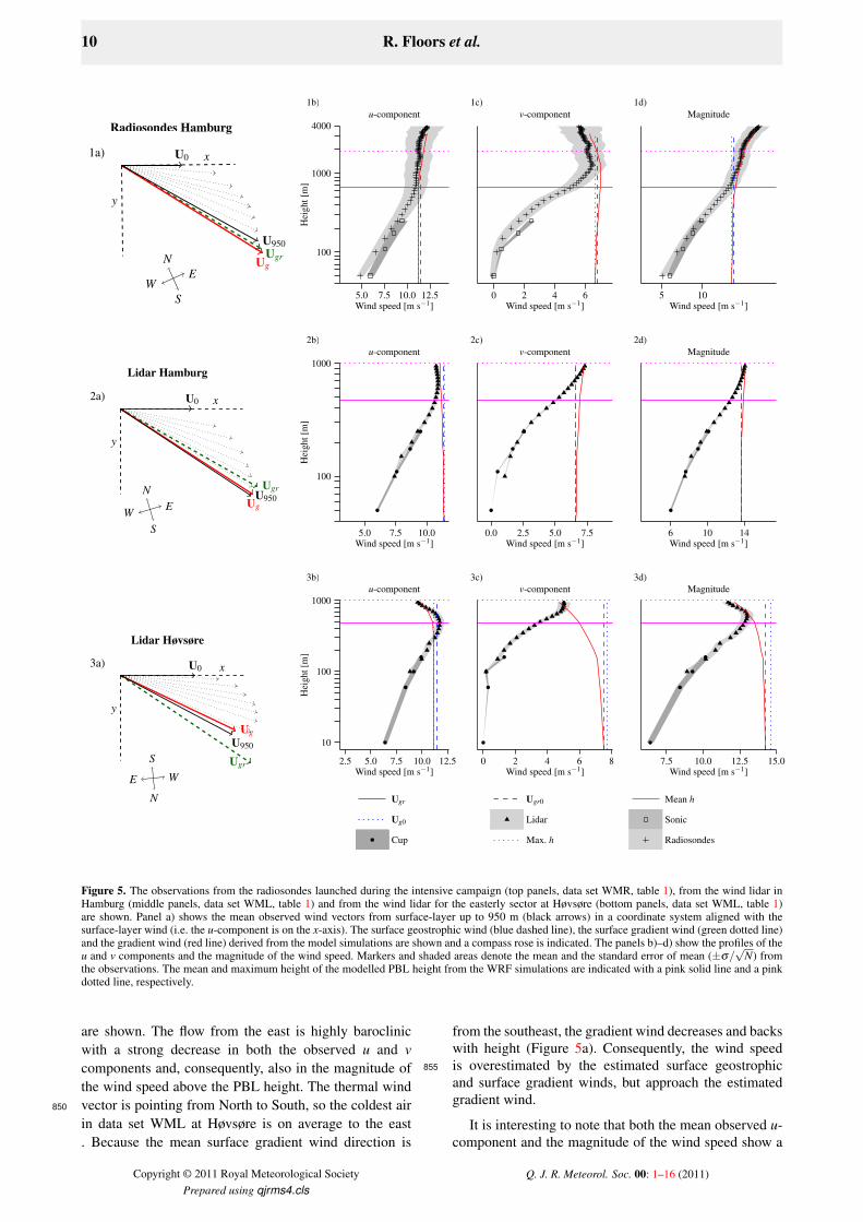
Table 2. Mean of the parameters of the geostrophic drag law using the neutral wind lidar profiles at Hamburg and Høvsøre (using data set WMLC,see Table 1).

Location N (-) A (-) σA (-) B (-) σB (-) φ (◦) h (m) u∗0 (m s−1) |UT | (m s−1) |Uh| (m s−1)Hamburg 563 0.00 2.27 4.03 2.50 22.49 663.93 0.67 1.78 16.56Høvsøre 52 1.54 2.84 4.84 2.68 25.86 683.57 0.55 3.28 16.53

account. During an intensive radio sounding campaign,the magnitude of the estimated gradient wind was foundto increase with height, which was also observed for theyearly mean wind profiles at Hamburg. At Høvsøre, the1040

wind aligned and perpendicular to the surface wind weredecreasing with height. This led to a wind profile stronglydecreasing in magnitude with height and, therefore, a jetformed with a wind speed maximum at around 500 m. Abaroclinic atmosphere, with suitably aligned gradient and1045

thermal winds can therefore generate frequent low-leveljets.

The observed wind veer from the surface up to thePBL height was shown to be a function of the anglebetween the surface gradient and the thermal wind. The1050

integration constants A and B from the geostrophic draglaw were derived using the surface-layer observations andthe observed wind at the PBL height. The mean valuesof A and B for the neutral PBL agreed well with earlierfield experiments on the neutral barotropic boundary1055

layer. However, the values of the constants were stronglydependent on the angle between the surface gradientwind and the thermal wind, a factor rarely considered inprevious studies of the geostrophic drag law.

Acknowledgements1060

We would like to thank three anonymous reviewers forconstructive comments and Robert Peel for help with theEnglish language. The study is supported by the DanishResearch Agency Strategic Research Council (Sagsnr.2104-08-0025) “Tall wind” project and the Nordic Centre1065

of Excellence programme CRAICC. The TEM section atDTU Wind Energy is acknowledged for maintenance ofthe data base for all measurements from the Høvsøre site.

References

Arya SPS, Wyngaard JC. 1975. Effect of Baroclinicity on Wind1070

Profiles and the Geostrophic Drag Law for the ConvectivePlanetary Boundary Layer. J. Atmos. Sci. 32(4): 767–778,doi: 10.1175/1520-0469(1975)032<0767:EOBOWP>2.0.CO;2,URL http://journals.ametsoc.org/doi/abs/10.1175/1520-0469(1975)032<0767:EOBOWP>2.0.CO;1075

2.Baas P, Bosveld F, Lenderink G, van Meijgaard E, Holtslag

AAM. 2010. How to design single-column model experimentsfor comparison with observed nocturnal low-level jets. Q. J.R. Meteorol. Soc. 136(648): 671–684, doi: http://doi.wiley.com/1080

10.1002/qj.592, URL http://doi.wiley.com/10.1002/qj.592.

Baas P, Bosveld FC, Klein Baltink H, Holtslag AAM.2009. A Climatology of Nocturnal Low-Level Jets atCabauw. J. Appl. Meteorol. Clim. 48(8): 1627–1642, doi:1085

10.1175/2009JAMC1965.1, URL http://journals.ametsoc.org/doi/abs/10.1175/2009JAMC1965.1.

Batchvarova E, Gryning SE. 2005. Progress in urban dispersionstudies. Theor. Appl. Climatol. 84(1-3): 57–67, doi: 10.1007/s00704-005-0144-1, URL http://link.springer.com/1090

10.1007/s00704-005-0144-1.

Blackadar AK, Tennekes H. 1968. Asymptotic Similarity in NeutralBarotropic Planetary Boundary Layers. J. Atmos. Sci. 25(6):1015–1020, doi: 10.1175/1520-0469(1968)025<1015:ASINBP>2.0.CO;2, URL http://journals.ametsoc.org/1095

doi/abs/10.1175/1520-0469(1968)025<1015:ASINBP>2.0.CO;2.

Brown A. 1996. Large-eddy simulation and parametrization of thebaroclinic boundary-layer. Q. J. R. Meteorol. Soc. 122(536):1779–1798, doi: 10.1256/smsqj.53602, URL http://www.1100

ingentaselect.com/rpsv/cgi-bin/cgi?ini=xref&body=linker&reqdoi=10.1256/smsqj.53602.

Brown AR. 1999. Large-eddy simulation and parametrization of theeffects of shear on shallow cumulus convection. Boundary-LayerMeteorol. 91(1): 65–80, doi: 10.1023/A:1001836612775.1105

Cariou JP, Boquet M. 2013. Leosphere Pulsed Lidar Principles.Technical report, Leosphere, 32 pp. Orsay, France.

Chen F, Dudhia J. 2001. Coupling an Advanced LandSurface–Hydrology Model with the Penn State–NCARMM5 Modeling System. Part I: Model Implementation1110

and Sensitivity. Mon. Weather. Rev. 129(4): 569–585, doi:10.1175/1520-0493(2001)129<0569:CAALSH>2.0.CO;2,URL http://journals.ametsoc.org/doi/abs/10.1175/1520-0493(2001)129<0587:CAALSH>2.0.CO;2.1115

Clarke RH, Hess GD. 1974. Geostrophic departure and the functionsA and B of Rossby-number similarity theory. Boundary-LayerMeteorol. 7(3): 267–287, doi: 10.1007/BF00240832, URL http://link.springer.com/10.1007/BF00240832.

Dudhia J. 1989. Numerical Study of Convection Observed during1120

the Winter Monsoon Experiment Using a Mesoscale Two-Dimensional Model. J. Atmos. Sci. 46(20): 3077–3107, doi:10.1175/1520-0469(1989)046<3077:NSOCOD>2.0.CO;2,URL http://journals.ametsoc.org/doi/abs/10.1175/1520-0469(1989)046<3077:NSOCOD>2.0.CO;1125

2.Floors R, Gryning SE, Peña A, Batchvarova E. 2011. Analysis

of diabatic flow modification in the internal boundary layer.Meteorol. Zeitschrift 20(6): 649–659, doi: 10.1127/0941-2948/2011/0290, URL http://dx.doi.org/10.1127/0941?1130

2948/2011/0290.Floors R, Vincent CL, Gryning SE, Peña A, Batchvarova E. 2013.

The Wind Profile in the Coastal Boundary Layer: Wind LidarMeasurements and Numerical Modelling. Boundary-LayerMeteorol. 147(3): 469–491, doi: 10.1007/s10546-012-9791-9,1135

URL http://link.springer.com/10.1007/s10546-012-9791-9.

Garratt JR. 1985. The inland boundary layer at low lati-tudes. Boundary-Layer Meteorol. 32(4): 307–327, doi: 10.1007/BF00121997, URL http://link.springer.com/1140

10.1007/BF00121997.Gryning SE, Batchvarova E, Floors R. 2013a. A study on the

effect of nudging on long-term boundary-layer profiles of windand Weibull distribution parameters in a rural coastal area.J. Appl. Meteorol. Climatol. 52(5): 1201–1207, doi: 10.1175/1145

JAMC-D-12-0319.1, URL http://journals.ametsoc.org/doi/abs/10.1175/JAMC-D-12-0319.1.

Gryning SE, Batchvarova E, Floors R, Peña A, Brümmer B, Hah-mann AN, Mikkelsen T. 2013b. Long-Term Profiles of Wind andWeibull Distribution Parameters up to 600 m in a Rural Coastal1150

and an Inland Suburban Area. Boundary-Layer Meteorol. 150(2):167–184, doi: 10.1007/s10546-013-9857-3, URL http://link.springer.com/10.1007/s10546-013-9857-3.

Hannesdóttir A. 2013. Boundary-layer height detection with aceilometer at a coastal site in western Denmark. Master thesis1155

m-0039, DTU Wind Energy, Roskilde, Denmark, Roskilde,


14 R. Floors et al.

Denmark, URL http://orbit.dtu.dk/services/downloadRegister/55566287/Boundary_layer_height.pdf.

Hess GD, Garratt JR. 2002a. Evaluating Models of The Neutral,1160

Barotropic Planetary Boundary Layer using Integral Measures:Part I. Overview. Boundary-Layer Meteorol. 104(3): 333–358,doi: 10.1023/A:1016521215844.

Hess GD, Garratt JR. 2002b. Evaluating Models Of The Neu-tral, Barotropic Planetary Boundary Layer Using Integral Mea-1165

sures: Part II. Modelling Observed Conditions. Boundary-LayerMeteorol. 104(3): 333–358, doi: 10.1023/A:1016521215844.

Hess GD, Hicks BB, Yamada T. 1981. The impact of theWangara experiment. Boundary-Layer Meteorol. 20(2): 135–174,doi: 10.1007/BF00119899, URL http://link.springer.1170

com/10.1007/BF00119899.Højstrup J. 1993. A statistical data screening procedure.

Meas. Sci. Technol. 4(2): 153–157, doi: 10.1088/0957-0233/4/2/003, URL http://stacks.iop.org/0957-0233/4/i=2/a=003?key=crossref.1175

967a06f9925c1959af7a8fa5e0afed8b.Holton JR, Hakim GJ. 2004. An introduction to dynamic meteorology.

Elsevier Academic press, 4th edn.Holtslag AAM. 1984. Estimates of diabatic wind speed profiles from

near-surface weather observations. Boundary-Layer Meteorol.1180

29(3): 225–250, doi: 10.1007/BF00119790, URL http://www.springerlink.com/index/10.1007/BF00119790.

Hong SY, Noh Y, Dudhia J. 2006. A New Vertical Diffusion Packagewith an Explicit Treatment of Entrainment Processes. Mon.Weather. Rev. 134(9): 2318–2341, doi: 10.1175/MWR3199.1,1185

URL http://journals.ametsoc.org/doi/abs/10.1175/MWR3199.1.

Hoxit LR. 1974. Planetary Boundary Layer Winds inBaroclinic Conditions. J. Atmos. Sci. 31(4): 1003–1020, doi:10.1175/1520-0469(1974)031<1003:PBLWIB>2.0.CO;2, URL1190

http://journals.ametsoc.org/doi/abs/10.1175/1520-0469(1974)031<1003:PBLWIB>2.0.CO;2.

Hu XM, Nielsen-Gammon JW, Zhang F. 2010. Evaluation ofThree Planetary Boundary Layer Schemes in the WRF1195

Model. J. Appl. Meteorol. Clim. 49(9): 1831–1844, doi:10.1175/2010JAMC2432.1, URL http://journals.ametsoc.org/doi/abs/10.1175/2010JAMC2432.1.

Joffre SM. 1982. Assessment of the separate effects of baroclinicityand thermal stability in the atmospheric boundary layer over1200

the sea. Tellus 34(6): 567–578, doi: 10.1111/j.2153-3490.1982.tb01845.x, URL http://doi.wiley.com/10.1111/j.2153-3490.1982.tb01845.x.

Kristensen L, Jensen G. 1999. Geostrophic Winds in Denmark: apreliminary study. Technical Report November, Risø National1205

Laboratory, Roskilde, Denmark.Larsén XG, Mann J. 2009. Extreme winds from the NCEP/NCAR

reanalysis data. Wind Energy 12(6): 556–573, doi: 10.1002/we.318, URL http://doi.wiley.com/10.1002/we.318.

Lenschow DH, Wyngaard JC, Pennell WT. 1980. Mean-Field1210

and Second-Moment Budgets in a Baroclinic, ConvectiveBoundary Layer. J. Atmos. Sci. 37(6): 1313–1326, doi:10.1175/1520-0469(1980)037<1313:MFASMB>2.0.CO;2,URL http://journals.ametsoc.org/doi/abs/10.1175/1520-0469%281980%29037%3C1313%1215

3AMFASMB%3E2.0.CO%3B2.Mlawer EJ, Taubman SJ, Brown PD, Iacono MJ, Clough SA. 1997.

Radiative transfer for inhomogeneous atmospheres: RRTM,a validated correlated-k model for the longwave. J. Geophys.Res. 102(D14): 16 663–16 682, doi: 10.1029/97JD00237,1220

URL http://www.agu.org/pubs/crossref/1997/97JD00237.shtml.

Münkel C, Schäfer K, Emeis S. 2011. Adding confidence levelsand error bars to mixing layer heights detected by ceilometer. In:Rem. Sens. Cl. Atmos. XVI, vol. 8177, Kassianov EI, Comeron1225

A, Picard RH, Schäfer K (eds). pp. 1–9, doi: 10.1117/12.898122,URL http://proceedings.spiedigitallibrary.org/proceeding.aspx?articleid=1269784.

Peña A, Floors R, Gryning SE. 2013a. The Høvsøre Tall Wind-ProfileExperiment: A Description of Wind Profile Observations in the1230

Atmospheric Boundary Layer. Boundary-Layer Meteorol. 150(1):69–89, doi: 10.1007/s10546-013-9856-4, URL http://link.springer.com/10.1007/s10546-013-9856-4.

Peña A, Gryning SE, Hahmann A. 2013b. Observations of theatmospheric boundary layer height under marine upstream flow1235

conditions at a coastal site. J. Geophys. Res. Atmos. 118(4): 1924–1940, doi: 10.1002/jgrd.50175, URL http://doi.wiley.com/10.1002/jgrd.50175.

Rotach MW, Vogt R, Bernhofer C, Batchvarova E, Christen A,Clappier A, Feddersen B, Gryning SE, Martucci G, Mayer1240

H, Mitev V, Oke TR, Parlow E, Richner H, Roth M, RouletYA, Ruffieux D, Salmond JA, Schatzmann M, Voogt JA.2005. BUBBLE – an Urban Boundary Layer MeteorologyProject. Theor. Appl. Climatol. 81(3-4): 231–261, doi: 10.1007/s00704-004-0117-9, URL http://link.springer.com/1245

10.1007/s00704-004-0117-9.Sathe A, Gryning SE, Peña A. 2011. Comparison of the atmospheric

stability and wind profiles at two wind farm sites over a longmarine fetch in the North Sea. Wind Energy 14(6): 767–780,doi: 10.1002/we.456, URL http://doi.wiley.com/10.1250

1002/we.456.Schotanus P, Nieuwstadt F, Bruin H. 1983. Temperature measurement

with a sonic anemometer and its application to heat andmoisture fluxes. Boundary-Layer Meteorol. 26(1): 81–93, doi:10.1007/BF00164332, URL http://www.springerlink.1255

com/index/10.1007/BF00164332.Seibert P, Beyrich F, Gryning SE, Joffre S, Rasmussen A,

Tercier P. 2000. Review and intercomparison of operationalmethods for the determination of the mixing height. Atmos.Env. 34(7): 1001–1027, doi: 10.1016/S1352-2310(99)00349-0,1260

URL http://linkinghub.elsevier.com/retrieve/pii/S1352231099003490.

Shary PA. 1995. Land surface in gravity points classification bya complete system of curvatures. Mat. Geol. 27(3): 373–390,doi: 10.1007/BF02084608, URL http://link.springer.1265

com/10.1007/BF02084608.Skamarock WC, Klemp JB, Dudhia J, Gill DO, Barker DM, Duda

MG, Huang XY, Wang W, Powers JG. 2008. A description of theAdvanced Research WRF version 3. Technical report, NCAR/TN-475+ STR, 113 pp. Mesoscale and Microscale Meteorology1270

Division, National Center for Atmospheric Research, Boulder.Sorbjan Z. 2004. Large-Eddy Simulations of the Baroclinic

Mixed Layer. Boundary-Layer Meteorol. 112(1): 57–80,doi: 10.1023/B:BOUN.0000020161.99887.b3, URL http://www.springerlink.com/openurl.asp?id=doi:1275

10.1023/B:BOUN.0000020161.99887.b3.Steyn DG, Baldi M, Hoff RM. 1999. The Detection of Mixed

Layer Depth and Entrainment Zone Thickness from LidarBackscatter Profiles. J. Atmos. Ocean. Tech. 16(7): 953–959,doi: 10.1175/1520-0426(1999)016<0953:TDOMLD>2.0.CO;2,1280

URL http://journals.ametsoc.org/doi/abs/10.1175/1520-0426(1999)016<0953:TDOMLD>2.0.CO;2http://journals.ametsoc.org/doi/abs/10.1175/1520-0426%281999%29016%3C0953%3ATDOMLD%3E2.0.CO%3B2.1285

Thompson G, Rasmussen RM, Manning K. 2004. ExplicitForecasts of Winter Precipitation Using an Improved BulkMicrophysics Scheme. Part I: Description and SensitivityAnalysis. Mon. Weather Rev. 132(2): 519–542, doi:10.1175/1520-0493(2004)132<0519:EFOWPU>2.0.CO;2,1290

URL http://journals.ametsoc.org/doi/abs/10.1175/1520-0493(2004)132<0519:EFOWPU>2.0.CO;2.

Tijm ABC, Van Delden AJ, Holtslag AAM. 1999. The inlandpenetration of sea breezes. Contr. Atmos. Phys. 72: 317–328, URL1295

http://ci.nii.ac.jp/naid/10013127286/en/.Troen I, Petersen EL. 1989. European Wind Atlas. Risø National

Laboratory: Roskilde, Denmark.Van Dijk A, Moene AF, De Bruin HAR. 2004. The principles

of surface flux physics: theory, practice and description of the1300

ECPACK library. Technical report, 99 pp. Meteorology andAir Quality Group, Wageningen University, Wageningen, theNetherlands.



Wilczak JM, Oncley SP, Stage SA. 2001. Sonic anemometer tiltcorrection algorithms. Boundary-Layer Meteorol. 99(1): 127–150,1305

doi: 10.1023/A:1018966204465.Xie B, Fung JCH, Chan A, Lau AKH. 2012. Evaluation of

nonlocal and local planetary boundary layer schemes in theWRF model. J. Geophys. Res. 117(May): 1–26, doi: 10.1029/2011JD017080, URL http://www.agu.org/pubs/1310

crossref/pip/2011JD017080.shtml.Zilitinkevich SS. 1975. Resistance Laws and Prediction Equations for

the Depth of the Planetary Boundary Layer. J. Atmos. Sci. 32(4):741–752, doi: 10.1175/1520-0469(1975)032<0741:RLAPEF>2.0.CO;2, URL http://journals.ametsoc.org/1315

doi/abs/10.1175/1520-0469(1975)032<0741:RLAPEF>2.0.CO;2.

Zilitinkevich SS, Esau IN. 2002. On integral measures of the neutralbarotropic planetary boundary layer. Boundary-Layer Meteorol.104(3): 371–379.1320

Zilitinkevich SS, Esau IN. 2003. The effect of baroclinicity on theequilibrium depth of neutral and stable planetary boundary layers.Q. J. R. Meteorol. Soc. 129(595): 3339–3356, doi: 10.1256/qj.02.94, URL http://doi.wiley.com/10.1256/qj.02.94.

Zilitinkevich SS, Esau IN. 2005. Resistance and heat-transfer laws for1325

stable and neutral planetary boundary layers: Old theory advancedand re-evaluated. Q. J. R. Meteorol. Soc. 131(609): 1863–1892,doi: 10.1256/qj.04.143, URL http://doi.wiley.com/10.1256/qj.04.143.


Documents

The effect of baroclinicity on the wind in the planetary