The Eï¬€ects of Government Ownership on Bank Lending

The Effects of Government Ownership

on Bank Lending

Paola Sapienza∗

Northwestern University & CEPR

This Draft: October 2002

Forthcoming: Journal of Financial Economics

Abstract

This paper studies the effects of government ownership on bank lending behavior.

Using information on individual loan contracts, I compare the interest rate charged to

two sets of companies with identical characteristics borrowing respectively from state-

owned and privately owned banks. State-owned banks charge lower interest rates than

do privately owned banks to similar or identical firms, even if the company is able to

borrow more from privately owned banks. State-owned banks mostly favor firms located

in depressed areas and large firms. The lending behavior of state-owned banks is affected

by the electoral results of the party affiliated with the bank: the stronger the political

party in the area where the firm is borrowing, the lower the interest rates charged. This

result is robust to including bank and firm fixed effects.

∗I am indebted to Andrei Shleifer for guidance and encouragement. I also thank Alberto Alesina, Paul

Armstrong-Taylor, Richard Caves, Riccardo DeBonis, Xavier Freixas, Anil Kashyap, Randy Kroszner, Patri-

cia Ledesma, Anna Paulson, Luigi Zingales, an anonymous referee, and seminar participants at 1999 European

Symposium in Financial Markets, NBER Universities Research Conference on Macroeconomic Effects of Cor-

porate Finance, American Finance Association, and the Federal Reserve of New York for helpful comments

and suggestions. Laura Pisani provided excellent research assistantship. All remaining errors are my respon-

sibility.

La Porta et al. (2002) document that worldwide, there is a large, pervasive government

ownership of banks. In 1995 the average percentage of state ownership in the banking

industry around the world was about 41.6 percent, and somewhat lower (38.5 percent) if we

exclude former socialist countries. Mayer (1990) shows that bank financing is the main source

of outside financing in all countries. Despite the prevalence of government-owned banks in

many countries, the prominent role of banks in financing enterprises, and the importance of

efficient financial markets for growth, there is very little evidence of the effects of government

ownership on bank lending.

In this paper I use a unique dataset on state-owned banks in Italy, where lending by

state-owned banks represents more than half of the total. By using data on interest rates

charged on individual loans, the paper studies the efficiency in the allocation of credit of

state-owned banks. Furthermore, I combine data on lending with the political affiliation

of the bank and results in recent elections to study the impact of political power on bank

lending behavior.

The debate concerning the role of ownership in banking is framed along the three al-

ternative theories of state-ownership, social, political, and agency views. The social view

(Atkinson and Stiglitz (1980)), which is based on the economic theory of institutions, sug-

gests that state-owned enterprises (SOEs) are created to address market failures whenever

the social benefits of SOEs exceed the costs. According to this view, government-owned

banks contribute to economic development and improve general welfare (Stiglitz (1993)).

In contrast, recent theories on the politics of government ownership (Shleifer and Vishny

(1994a)) suggest that SOEs are a mechanism for pursuing the individual goals of politicians,

such as maximizing employment or financing favored enterprises. The political view is that

SOEs are inefficient because of the politicians’ deliberate policy to transfer resources to their

supporters (Shleifer (1998)).

The agency view shares with the social view the idea that SOEs may be created to

maximize social welfare, but may generate corruption and misallocation (Banerjee (1997)

and Hart, Shleifer, and Vishny (1997)). Agency costs within government bureaucracy may

result in weak managerial incentives in SOEs. According to this view, the ultimate efficiency

1

of SOEs depends on the trade-off between internal and allocative efficiency (Tirole (1994)).

These theories cannot be disentangled by looking at bank profitability: it is not clear

whether government owned banks are less profitable because they maximize broader social

objectives, because they have lower incentives, or because they inefficiently cater to politi-

cians’ wishes. The empirical strategy I use in this paper addresses these problems. Instead of

looking at overall bank performance, where the mix of activities performed by banks might

change under government ownership, I focus on the lending relations of the banks. The data

I use include information on the balance sheets and income statements of a panel of over

37,000 Italian firms. The data are collected by Centrale dei Bilanci (CdB), an institution

created to provide its members, mainly banks, with economic and financial information for

screening Italian companies. For a large subset of the 37,000 companies, CdB members re-

ceive a numerical score, which CdB obtains by using traditional linear discriminant analysis,

to identify the risk profile of the companies (Altman, 1968). I merge this information with

data on the credit relations of the firms surveyed in the CdB database.

The information in this database is available to all the banks prior to lending and has

proven to be very accurate in predicting the success or failure of a company (see Altman

et al. (1994)). Since both privately owned and state-owned banks have access to the same

information, I can use this system to check the differences in the credit policies of the various

banks.

I look at the individual loan contracts of the two types of banks. I compare the interest

rate charged to two sets of companies with identical scores which are borrowing either from

state- or privately owned banks, or both. My main result is that, all else equal, state-owned

banks charge lower interest rates than do privately owned banks. On average, the difference

is about 44 basis points.

I claim that this difference can best be explained by the political view of state-owned

firms. First, my results show that even companies that are able to access private funds

benefit from cheaper loans from state-owned banks. Second, companies located in the south

of Italy benefit more than companies located in the north from borrowing from state-owned

banks, consistent with the view that political patronage is more widespread in the south

2

(Ginsborg (1990)). This result remains true controlling for the presence of credit constraints.

Finally, contrary to the social welfare maximizing view, state-owned banks are more inclined

to favor large enterprises. Overall, my results support the political view of government

ownership. However, I note that some of these results can also be consistent with some

versions of the social view and the agency view. For example, one could argue that firms

located in the south receive cheaper funds because a socially maximizing government wants

to channel funds in depressed areas of the country. My findings that larger firms get cheaper

funds may be also consistent with the agency view.

To further distinguish among the different theories, I analyze the relation between interest

rates, the political affiliation of the bank, and electoral results. I find that the lending

behavior of state-owned banks is affected by the electoral results of the party affiliated with

the bank: the stronger the political party in the area where the firm is borrowing, the

lower the interest rates charged. This result is not driven by omitted banks’ and firms’

characteristics, since I show that it is robust to including both bank and firm fixed effects.

Overall, my results support the political view of SOEs and suggest that state-owned

banks serve as a mechanism to supply political patronage. These results relate to important

policy debates. My finding show that government ownership of banks has distorting effects

on financial allocation of resources. This is consistent with findings that widespread state

ownership of banks is correlated with poor financial development (Barth, Caprio and Levine,

2000). In turn, a highly politicized allocation of financial resources may have deleterious

effects on productivity and growth, as recent research by La Porta, Lopez-de-Silanes, and

Shleifer (2002) shows.

The paper is organized as follows. The next section briefly outlines the theories of SOEs

and their predictions. Section 2 provides a description of the institutional environment.

Section 3 describes the data, the sample, and the methodology. Section 4 presents the

empirical evidence. Section 5 concludes.

3

I Theoretical issues

The three main views of SOEs – social, agency, and political – have different implications for

both the existence and the role of state-owned banks. The social view sees SOEs as institu-

tions created by social welfare maximizing governments to cure market failures. According

to this view, state- and privately owned enterprises differ because the first maximizes profits

and the latter maximizes broader social objectives. In this literature, the reason for creating

public financial institutions is the existence of market failures in financial and credit markets

(Stiglitz and Weiss (1981), Greenwald and Stiglitz (1986)). Thus, creating state-owned banks

or programs of direct credit has often been justified on the ground that private banks fail

to take social returns into account. For example, private banks may not allocate funds to

projects with high social returns or to firms located in specific industries (Stiglitz (1993)).

Under the social theory, the objective function of state-owned banks should be to channel

resources to socially profitable projects or to firms that do not have access to other funds.

The agency view shares with the social theory the idea that governments seek to max-

imize social welfare. Under the agency hypothesis, governments design public financial in-

stitutions to cure market failures. However, since SOEs maximize multiple nonmeasurable

objectives, managers of SOEs have low-powered incentives (Tirole (1994)).1 Given the incen-

tive problems associated with the control of SOEs, the agency view concludes that decisions

on government in-house provision of public goods should depend on the trade-off between in-

ternal and allocative efficiency. Under this hypothesis, state-owned banks channel resources

to socially profitable activities, but public managers may exert less effort (or divert more

resources) than would their private counterparts. The agency view predicts that in general

state-owned banks serve social objectives and allocate resources where private markets fail.

However, public managers of state-owned banks may exert low effort or divert resources for

personal benefits, for example, for career concerns, with an eye towards future job prospects

in the private sector.

According to both the social and the agency view, the government role in the economy

1Low powered incentives are not always bad. Laffont and Tirole (1993) show that, under some circum-

stances, a concern for quality calls for low powered incentives.

4

emerges and evolves to perform the economic functions that markets either cannot handle or

cannot perform well. Fundamentally different, the political view is based on the assumption

that politicians are self-interested individuals who pursue personal, political, and economic

objectives rather than maximizing social welfare. The main objective of politicians is to

maintain voting support. Hence, SOEs provide jobs for political supporters, and direct

resources to friends and supporters (Shleifer and Vishny (1998)). According to this view,

politicians create and maintain state-owned banks not to channel funds to economically

efficient uses, but rather to maximize politicians’ personal objectives.

Though the agency and the political views make very different assumptions about gov-

ernment’s objectives, the difference in the empirical implications is not so clearly defined.

The merit of the agency view is to show that misgovernance can exist even when the govern-

ment has the best of intentions (see Banerjee (1997)). Under both views, we would observe

some misallocation of resources, but for different reasons. The agency view claims that the

misallocation takes place because managers shirk or divert resources for their private use, but

under the political view, the misallocation of resources is the objective of politicians, rather

than due to the lack of incentives. State-owned banks will divert resources to areas where

there is more political patronage, will finance friends and supporters of politicians, and will

maximize political support, e.g., maximize employment at the bank level or at other firms.

II State ownership of banks in Italy

Though there are more privately owned banks than state-owned banks in Italy (864 compared

to 117), in 1995 the percentage of total assets held by state-owned Italian banks was 58

percent, among the highest in the industrialized world.2 But, Italy is not unique in this

dimension: most Continental European countries are similar (e.g., in Germany the proportion

is 50 percent, in France, 36 percent). Latin American countries also show a very high

percentage of state ownership. In fact, in a recent paper La Porta et al. (2002) show that

worldwide, there is a large, pervasive government ownership of banks. In 1995 the average

percentage of state ownership in the banking industry around the world was about 41.6

2I consider foreign banks operating in Italy as being privately owned.

5

percent, and somewhat lower (38.5 percent) if we exclude former socialist countries.

Data on Italian state-owned banks suggest that, in general, they have a different lending

focus from privately owned banks. De Bonis (1998) shows that state-owned banks make more

than 11 percent of their loans to state or local authorities (compared to 1.6 percent loaned by

private banks). The percentage loaned to companies is similar between state- and privately

owned banks (55.1 and 57.5, respectively), but no analysis has investigated the differences

within each class of borrowers for the two groups of banks. De Bonis (1998) also finds that

state-owned banks are less profitable in making loans than are privately owned banks. In

1995, the percentage of bad loans on bank capital for state-owned banks was 57.2, almost

double of that of private institutions (30.2 percent).

The degree of political influence on state-owned banks is evident in the procedure used to

appoint the chairpersons and top executives in state-owned banks. Until 1993, the appoint-

ments of the directors and management of the banks was made by a specific Parliamentary

commission.3 For example, in 1992, this commission met three times: on October 30th

they appointed 72 of chairpersons, vice-chairpersons, and CEO of state-owned banks; on

December 1st they appointed other 26, and on December 30th an additional 33.

Over time there could have been differences in the level of political interference. Some

authors (e.g., Barca and Trento (1994) and Ginsborg (1990)) claim that close personal ties be-

tween party leaders and the managers of SOEs were introduced after the mid 1950s. De Bonis

(1998) claims that the management of state-owned banks became independent from the cen-

tral government after 1993, when the public entities that previously owned the banks directly

were transformed into foundations. Nonetheless, some observers believe that the practice of

political appointments of top executives in state-owned banks has survived (e.g.,Visentini,

2000).

3Specifically, the Comitato Interministeriale per il Credito e il Risparmio (CICR), a permanent Parlia-

mentary commission, in which the political groups are represented according to their relative strength in

Parliament.

6

III Data and Methodology

In this study, I rely on several data sources. The two main databases come from Company

Accounts Dataset (CAD) and the Credit Register (CR). CAD reports balance sheet and

income statements for more than 50,000 Italian companies. CR collects information about

any individual loan contracts over 80 million lire (about 41,300 Euro) granted by banks to

any customer. This information is readily available to the CdB membership, which is mainly

comprised of banks. Starting in 1991, CdB also developed what it called the Diagnostic

System, which was designed to provide banks with a tool for quickly identifying the soundness

of the companies included in the database. This system applies traditional linear discriminant

analysis based on two samples of businesses of healthy and unsound companies. A numerical

score is obtained from two discriminant functions. This score summarizes the “risk profile” of

the business. This system has proven to be very successful: it correctly classified in the year

immediately prior to distress 87.6 percent of healthy companies and 92.6 percent of unsound

companies (see Altman et al. (1994)). Appendix I provides more details on the numerical

score.

For each firm, the CR reports the amount of credit granted by each bank, together with

the amount used (outstanding balance). In addition, 90 banks (accounting for over 80 percent

of total bank lending) agreed to file detailed information about the interest rates charged on

each loan. These data, collected for monitoring purposes, are highly confidential.

A subset of CR data includes all the companies that were surveyed for at least one year in

CAD. Data on loan contracts are quarterly, but data on balance sheets and income statements

are annual. Aggregate information on bank balance sheets and income statements comes

from the prudential supervision statistical data, where it is reported on a quarterly basis. I

constructed the data on the bank ownership by using the Bank of Italy legal classification

prior to 1990.4

I obtain local election results for three national elections, 1989, 1992, and 1994 from the

4Prior to 1990 all state-owned banks had a different legal status from private banks (either corporations

and cooperatives). After 1990, all the state-owned banks’ charters were modified by law and banks were

transformed into corporations.

7

archives of the Interior ministry. The local unit is the province (similar to U.S. counties).

The archives provide the total valid votes and the votes collected by all the parties running

the elections in each of Italy’s 95 provinces.

I collect the data on political affiliation of the top management of the bank from newspa-

pers. For 36 state-owned banks I am able to identify the political affiliation of the chairperson.

Appendix II provides additional details about these data and the electoral data.

A Privately owned and state-owned banks

The data on loan contracts come from the subset of the CR and CAD datasets previously

described. The sample period begins in 1991 and ends in 1995, because 1991 is the first year

in which CAD distributed the information on the score to its members. I restrict my attention

to privately owned and state-owned banks that file information about interest payments and

are members of the CdB.

This criterion introduces a potential sample selection, since the banks that file interest

rate information are generally larger than the average Italian bank. However, it turns out

that this is not a problem for the sample of state-owned banks: the sample represents more

than 90 percent of state-owned loans. I exclude small state-owned banks from the sample, but

they are not the typical state-owned bank. Privately owned banks selected with these criteria

are larger than the average privately owned bank, but because I use them as benchmark for

comparing the behavior of state-owned banks, it is important that they are similar in size to

the state-owned banks.

These selection criteria restrict the total number of banks to 85: 40 have always been

privately owned; 43 are state-owned banks; and two are privatized during the period of

observation.

Table 1 shows descriptive statistics of the banks in the sample. The median state-owned

bank has a ratio of non-performing loans to total loans of 6.91 percent, as opposed to 5.25

percent for privately owned banks. The mean for the two sub samples is statistically different

at 1 percent level of significance. State-owned banks also have a lower return on assets

(0.34 for the median state-owned bank, as opposed to 0.51 for the median privately owned

8

bank) and higher operating costs over assets (3.05 for the median state-owned bank, as

opposed to 2.87 for the median privately owned bank). These differences in the sample

reflect differences between state-owned and privately owned banks and represent a potential

problem in comparing credit policies of these two sub-samples of banks.

B Companies borrowing from privately owned and state-owned banks

Ideally, I would like to compare the entire loan portfolio of state-owned and privately owned

banks and, using the balance sheet and income statement information for the companies,

compare the credit decisions of these two types of banks. Unfortunately, the information on

the firms’ characteristics is available only for a subset of the companies that receive credit

from the banks.

To deal with this lack of information, I take a different approach. Instead of comparing

the entire loan portfolio of state-owned and privately owned banks, I compare two matching

samples of companies that borrow from state and privately owned banks, respectively. The

advantage of using this approach is that I can compare the interest rate charged in the

same period to the same company, or to very similar companies, by state- and privately

owned banks (many firms have credit ties with both types of banks). Since state- and

privately owned banks have access to the same information for evaluating these companies,

any difference in the price of the loan is likely to reflect differences in the objective of the

bank, rather than differences in the evaluation skills of the banks’ loan officers.

To select the sample of companies in this study, I use the following criteria: from the

sample of companies included in CdB, I select a subsample of companies that have a loan with

at least one bank in the sample for at least one period and for which there is a numerical score.

Because loan characteristics (collateral, etc...) may have an impact on loan rates (Petersen

and Rajan, 1994, and Berger and Udell, 1994) I focus on homogenous loan contracts. I

analyze credit line contracts, the most common loan contract in Italy in which banks set

the amount of loan money granted and an interest rate. The loans analyzed here exclude

long-term loans, collateralized, and subsidized loans.5.

5There are other characteristics of the relationship between banks and borrowers that I cannot control

9

From this data I select the subset of companies that have been borrowing from state-

owned banks. For each observation in this sample (company-bank-year) I identify a matching

company that borrows from a privately owned bank in the same period. Whenever the

company borrows in the same year from both state- and privately owned banks, I match the

company with itself. If a company borrows only from state-owned banks, I choose a similar

firm that borrows from privately owned banks in the same year. In these cases, I identify the

matching company as a firm operating in the same industry and in the same geographical

area (north, center, and south), with an identical risk profile (Altman’s z-score (Altman,

1968, 1993)), and similar size (measured by sales). I also require that if the company that

receives loans from state-owned banks is state-owned (privately owned), then the matching

company is state-owned (privately owned) as well.

These selection criteria reduce the sample to a total of 6,968 companies, corresponding

to 110,786 company-bank-year observations. 55,393 observations refer to borrowers of state-

owned banks and 55,393 to borrowers of privately owned banks.

By construction, the companies that borrow from state- and privately owned banks have

identical scores, operate in identical industries, and are located in the same geographical

area. Table 2 shows the sample scores for the two sub-samples of companies.

The summary statistics on the two sub-samples of firms (Table 3) also show that the

selected companies borrowing from state- and privately owned banks are very similar. None

of the differences in the means of the relevant variables is statistically significant. In both

sub-samples, the median firm has 58 employees, 21 billion lire in sales, 18 billion lire in

assets and a coverage, interest expenses divided by EBITDA, of 1.47. The median firm has

a leverage of 71 percent. I define leverage as the book value of short plus long term debt

divided by sum of the book value of short plus long term debt and the book value of equity.

Return on sales is slightly below 8 percent. The majority of the companies are privately

for. Although the loan contracts included in the sample have homogenous characteristics, borrowers might

have contemporaneous contracts with the bank (deposits, collateralized loans) that might affect the cost of

the loan. Also, the quality of service or the probability of the loan to be revoked can vary across banks.

Unfortunately, I cannot rule out any of these possibilities; therefore my results should be interpreted with

these caveats in mind

10

held. Seventy are state-owned companies.

IV Empirical analysis

A Differences in interest rates

To learn whether state- and privately owned banks behave differently, I examine the interest

rate charged to similar companies by these two types of banks. I first compare the average

interest rates charged by both types of banks and then present a regression analysis that

controls for banks’ and firms’ characteristics.

Table 3 reports the average interest rate minus prime rate charged by both types of banks.

I define the interest rate as the ratio of the quarterly payments made by the firm to its bank

(interest plus fixed fees) to the firm’s quarterly loan balance. Of course, this measure of

interest rate overestimates the interest rate of a firm with a small average balance. For this

reason, I eliminate the rates linked to credit lines with less than 50 million lire in average

daily balance. The same criterion has been used by Pagano et al. (1998) and Sapienza

(2002).

Column 3, table 3 presents the differences in the interest rates minus the prime rate for

the two subsets of banks (i.e. column 2 minus column 1). For the overall sample, these

comparisons show that for similar companies, the average interest rate charged by state-

owned banks is lower than that charged by private banks. The differences are statistically

significant in a t-test.

Table 3 also presents the differences in interest rates for various risk profiles of the compa-

nies, demonstrating that these differences are not driven by few outliers. Also, to make sure

that the differences are not driven by any incorrect matching, panel B of Table 3 presents

the same statistics for the subsample of firms that borrow from both state- and privately

owned banks during the same year (the matching firm is self).

My main finding is that for any risk profile, the interest rate charged by state-owned

banks is lower than that charged by privately owned banks. The difference in interest rates

is statistically significant at 1 percent level.

11

The average difference between the interest rates charged by private and state-owned

banks is 23 basis points. However, the comparisons presented above are not conditioned on

other characteristics of the banks, such as differences in size and riskiness of the portfolio.

Table 1 shows that state- and privately owned banks are different in size, profitability, and

riskiness. To address this issue, I use a regression model to estimate the difference in interest

rates charged by the two types of banks.

I regress rikt, the relative interest rate charged at time t by bank k to company i (defined

as the interest rate minus the prime rate) on a dummy variable, STATEk,t, that equals

one if at time t bank k is a state-owned bank. The coefficient measures the impact of state

ownership on interest rates. A negative (positive) value means that state-owned banks charge

a lower (higher) interest rate than do privately owned banks. I also include several regressors

to control for firms’, market’s, and banks’ characteristics. Finally, I include a vector of time

fixed effects and a vector of firm fixed effects. By using a firm fixed effect, I compare the

interest rate charged by various banks to the same company.

Panel A, Table 4, reports the regression results. Heteroskedasticity-robust standard errors

are shown in parentheses. I also adjust standard errors for within-year clustering. Column

1 reports the estimates of the interest rate regressed on the STATEk,t dummy and time

and firm fixed-effects. These results are directly comparable to the simple differences in the

last row of Table 3: state-owned banks charge interest rates 23 basis points lower than do

privately owned banks.

As mentioned before, the coefficients measuring state ownership may capture specific

characteristics of state-owned banks and local market structure. To overcome this problem,

in columns 2 to 5 of Table 4, I include several other controls.

In column 2 I introduce a proxy for the size of the bank, measured by logarithm of bank’s

total assets. Aside for the part size plays in determining market concentration measures,

a bank’s size should affect prices according to the theoretical literature. For example, in a

standard Cournot model with capacity constraints (increasing returns to scale), one can show

that the bank with lower capacity would supply loans equal to capacity at a lower price than

the other bank with higher capacity (see Tirole, 1989). Size may also reflect some implicit

12

characteristics of the loan. Loans from large banks may carry an implicit guarantee of not

being revoked, if large banks are perceived to be less likely to fail. Empirically, Sapienza

(2002) finds that bank’s size has a positive and significant effect on loan rates for a sample

of privately-owned banks, after controlling for firms’ characteristics. Column 2 of Table 4

confirm this result. All else equal, a one-standard-deviation increase in the logarithm of

banks’ assets leads to an increase of nearly 14 basis points in the interest rate. Since state-

owned banks are generally larger than privately owned banks, the size of the coefficient of

STATEk,t increases from .23 to.46 after I control for banks’ size, suggesting that the mean

differences in Table 3 underestimate the impact of state ownership.

In column 3 of Table 4 I include two other controls in the regression. First, I include a

measure of market concentration (the Herfindahl-Hirschman Index on loans) as many studies

have identified a positive relationship between market concentration and prices (Berger and

Hannan (1989) and Hannan (1991). Another potential problem in my basic regression is that

the state-ownership dummy captures the fact that banks with a higher proportion of non-

performing loans charge lower rates. For example, riskier banks may offer loans of inferior

quality, with higher probability of being revoked. For this reason, I include a measure of the

riskiness of the bank (the percentage of non-performing loans).

The Herfindahl-Hirschman Index (HHI) on loans has the predicted effect. One standard

deviation increase in HHI increases interest rates by 7 basis points. Surprisingly, the effect of

the percentage of non performing loans is positive and significant. A one standard deviation

increase in the percentage of non-performing loans causes a 13 basis points increase in interest

rates. The regression predicts that, other else equal, a firm would save 50 basis points on

loans from state-owned banks.

Consistent with the benign view of government, state-owned banks may forego exploiting

market power when they possess it, while private ones will not. In fact, in column 4 I consider

this possibility and re-estimate the regression, interacting the state-ownership dummy with

the HHI. The results show that state-owned banks do in fact exploit market concentration

less than otherwise similar private banks. Moving from the area with the lowest HHI to the

area with the highest HHI private banks increase rates by 63 basis points, while state-owned

13

banks increase rates by 44 basis points. This difference in behavior does not explain the

systematic difference found between private and state-owned banks rates. First, the results

show that state-owned banks exploit market power, only to a lesser extent than private

banks. Second, the difference is small, in the province with the median HHI, everything else

being equal, state-owned banks rates are lower than private banks rates by 6 basis points.

Finally, the coefficient of the state-ownership dummy remains statistically and economically

significant. After controlling for differences in market power exploitation, I find a difference

of 44 basis points in rates charged between private- and state-owned banks.

As a further check for robustness, the specification in column 5 introduces the size of the

firm (measured by logarithm of sales) and score. Although both the coefficients of the size of

the firm and of the numerical score are statistically significant and have the right sign, the

size of the estimated state ownership dummy does not change.6

One potential worry is that the results may be entirely attributable to unobservable firms’

characteristics that may be changing over time. If that is the case the firm fixed effect is not

fully controlling for this. To address this point, however, I can use one important feature of

my data. I constructed the sample in such a way that a large percentage of companies in the

sample receive loans from both state- and privately owned banks during the same year. To

ensure that the results presented above hold for the companies that borrow from both types

of banks at the same time, I re-estimate the regression model for this subsample of companies

only. Panel B, Table 4, presents the results, which show a negative and significant coefficient

for the STATEk,t dummy. All else equal, firms that raise money from both state-owned

and private banks pay interest rates to state-owned banks that are lower by 44 basis points,

confirming that the results cannot be attributable to unobservable firms’ characteristics.

B Discussion

Table 4 shows that when I control for firms’ and banks’ characteristics, state-owned banks

charge interest rates that are 44 basis points lower than those charged by comparable privately

6I have also estimated some alternative specifications that include, among the regressors, other firms’

control variables (i.e. leverage and profitability). The substantive results (unreported) are unchanged.

14

owned banks.

This result supports many alternative hypotheses. First, consistent with the political

view, state-owned banks may be charging lower interest rates to some firms because this

responds to the politicians’ objectives. For example, the firms that benefit from lower rates

may be political supporters of the politicians.

Even if politicians maximize social welfare, managers of state-owned banks may lack the

ability to screen firms. If bank managers systematically make mistakes in pricing loans,

in equilibrium we observe only public loan contracts with lower interest rates, because the

entrepreneurs will choose the contracts with the lowest interest rates. Also, managers of

state-owned banks may be diverting banks’ resources to their own benefit, favoring firms

that bribe them or offer other types of benefits in exchange (e.g., future jobs). These latter

two interpretations support the predictions of the agency view.

Are the results in Table 3 and 4 consistent with the social view? One problem with

answering to this question is that the social view is pretty vague on the specific social wel-

fare maximizing tasks that a state-owned bank is likely to perform. So, in the remaining

paragraphs of this section, I will explore several potential objectives of state-owned banks

according to the social view.

One way to explain the difference in interest rates is to claim that state-owned banks

are either more efficient than privately owned banks or have lower costs, and thus are able

to charge lower interest rates. During the period of observation, regulation and tax laws

are identical for both state- and privately owned banks, so the argument that state-owned

banks are more efficient in making loans should be based on the fact that state-owned banks

are better managed organizations. The data do not confirm this hypothesis. It is well

documented in the literature that state-owned Italian banks are less efficient than their

private counterparts (see Martiny and Salleo (1997)). Table 1 confirms this fact for my

sample.

The central prediction of the social view is that to cure market failures benevolent public

banks are willing to lend to companies at lower interest rates. According to this view, state-

owned banks favor enterprises that find it difficult or too expensive to raise capital from

15

private banks. This argument assumes implicitly that state-owned banks make loans to

companies with positive net present value (NPV) that are unable to raise capital from other

sources. As it turns out, the data contradict this hypothesis.

The results in Table 4, Panel B show that state-owned banks charge lower interest rates

even if the firm is able to raise capital from alternative sources. However, one could argue

that these companies are rationed in terms of the funds they get from the private banks.

To consider this possibility, I look at the ratio of the outstanding balance to the available

amount (credit line) offered by privately owned banks. To prove that these companies are

rationed, I must show that the outstanding balance is equal to the credit line. In fact,

on average, the companies that borrow from privately owned banks have a percentage of

loan use below 14 percent, suggesting that they could borrow larger amounts from privately

owned banks. To further explore this issue, I restrict the sample to companies that borrow

from both state-owned and private banks and have unused credit lines with private banks.

The estimates (not reported) confirm the previous results. In Table 4, Panel C I also check

whether firms that use a bigger fraction of their line of credit from private banks (and thus

are more constrained) receive a bigger discount from state-owned banks. In column 1, 2, and

3 of Table 4, Panel C I report the results of the baseline regression where I add a new dummy

that is equal to one if the bank is state owned and if the firm has an average percentage

of used credit from private banks that exceeds a given threshold. As thresholds, I use 15

percent (75th percentile), 37 percent (95th percentile), and 72 percent (99 percentile). All

the reported results show that the new dummy has a positive and insignificant coefficient.

These findings suggest that the firms receiving lower rates from state-owned banks are able

to raise capital form other private banks.

An alternative scenario consistent with my findings may support the social view. The

government could wish to subsidize certain firms (e.g., firms that have difficulty accessing

capital) by reducing the firm’s average cost of capital. However, to maintain incentives, the

government might want the firm to face the market interest rate at the margin. In this case,

the government might offer a loan below the market rate for less than the full size of the

project. The initial loan granted by the state-owned bank could then trigger more loans by

16

private banks. Unfortunately, I am not able to test this hypothesis with my data because I

do not have information on when the loans are initiated.

Concluding, the results presented in Table 4 are consistent with all the three views of

SOEs.

C Sub-sample analysis: Geographic location and firm size

To further investigate the behavior of state-owned banks and distinguish among the different

theories, I study whether there is some class of borrowers that has a greater advantage in

borrowing from state-owned banks. I look at two different dimensions: geographical location

and size of the companies. I focus on the subsample of firms that receive loans from both

state-owned and private banks. By doing this, I exclude firms that may face it difficulties

obtaining loans in the private market.

As a first approximation, Table 5 presents the average interest rates charged by state-

owned and private banks to the firms that borrow from both types of banks. The first

three rows divide the sample according to the geographical location of the companies. The

differences between the interest rates charged by private banks and state-owned banks suggest

that companies located in the south of Italy benefit more than do other companies from

borrowing by state-owned banks, even when they have access to private funds.

Table 6 looks at the same issue from within a regression framework. Table 6 presents

the results of regression (1) including an interaction between companies’ location and the

STATEk,t dummy. For firms located in northern Italy (the omitted indicator), borrowing

from state-owned banks saves 44 basis points, all else equal. For firms located in the south,

a relationship with the state-owned bank would save them 75 basis points. This finding is

consistent with Alesina, Danninger, and Rostagno (1999), who find that public employment

in Italy is used as a subsidy from the north to the less wealthy south.

It is hard to reconcile this result with the incentive view. There is no particular reason

why the managers of state-owned banks should have weaker incentives when they price loans

to firms located in the south.

By contrast, both the social and the political views support the fact that state-owned

17

banks apply higher discounts to firms located in the south of the country. The south of

Italy is the poorest part of the country with an unemployment rate four times higher than

in the center-north. For at least fifty years the south has been the focus of regional devel-

opment policy, with massive capital inflows and real income transfers from the government.

Lower interest rates to southern firms are consistent with a policy of subsidization, aimed

at stimulating the southern regions.7 On the other hand, in the south the practice of po-

litical patronage is more widespread than in the north. Southern politics in Italy is largely

organized around the distribution of patronage (see Golden (2001) and Ginsborg (1990)).

This evidence suggests that there is another reason why firms located in the south are fa-

vored by the interest rate policy of state-owned banks: such favorable terms may be due to

state-owned banks pursuing political objectives.

Table 5 also reports the differences across firm size in the interest rates charged by

state- and privately owned banks. The results show that on average, the largest firms have

more advantages in borrowing from state-owned banks. The difference between the interest

rates charged by privately owned and state-owned banks is higher for the companies in the

largest quintile. The relation across quintiles is nearly monotonic, but the differences are not

statistically significant across quintiles.

Table 7 looks at the same issue in a regression framework. The results confirm that state-

owned banks favor larger enterprises. The reduction in interest rates applied to companies

in the largest quintile (the omitted indicator) by central government-owned banks is around

55 basis points. Firms in the smallest quintile that borrowing from state-owned banks save

about 41 basis points, all else equal.

This result does not support the social view. If market imperfections prevent firms

from raising money, then the benevolent state-owned banks should charge relatively lower

interest rates to small companies that are more likely to be credit rationed.8 Instead, the

7The fact that these subsidization policies have systematically failed to close the gap between the center-

north and the south raises some doubts on the rationale of the development policy for the south. Nonetheless,

perhaps ex-ante the government undertook these policies to maximize social welfare.8Other evidence against the social view is that state-owned banks do not favor any particular industry.

In another (unreported) regression I look at differences in interest-rate discounts across industries. I use the

Rajan and Zingales (1998) measure of external financial dependence and check whether firms in industries

18

results appear to support both the agency view and the politicians view. Managers of state-

owned banks who lack incentives may be more prone to favor larger enterprises because their

personal rewards are likely to be higher (e.g., a career in a larger firm is more valuable than

one in a smaller firm). At the same time, state-owned banks may favor large enterprises,

because state-owned banks are interested in maximizing a larger political consensus.

To sum up, while the social view and the incentive view alone can explain some results,

the only interpretation consistent with both results is the political view of SOEs.

D Electoral results, party affiliation, and lending behavior

To clarify the relationship between politicians’ objectives and the lending behavior of state-

owned banks, I collect data on the political affiliations of the top executives of state-owned

banks. Ideally, I would like to link the credit policy of the bank to the political affiliation

or voting behavior of the beneficiaries of the loans. Unfortunately, this information is not

publicly available. Instead, I use the voting record of the province where the borrower is

located. Although this is an approximation, it provides new insights on the influence of

politics on SOEs.

Because I am interested in the relationship between the party affiliation of state-owned

banks and lending behavior in this section I focus only on the subsample of firms that borrow

from state-owned banks. I determine the political affiliation of 36 state-owned banks in my

sample (not always for the whole sample period).9 I focus on the political affiliation of the

chairpersons. I do so because in Italian state-owned banks, the chairperson has strategic

tasks and often acts as the CEO. Overall, in my sample the affiliation of the chairperson is

linked to five different parties (See Appendix II for details). The political affiliations of the

chairperson of the state-owned banks are relatively stable over time. In only four of the 36

banks does the political affiliation change during the sample period.

I use provincial electoral results from three national elections (1987, 1992, and 1994).

that are more dependent on outside funds receive cheaper loans from state-owned banks. In contrast to the

social view, the results do not support this hypothesis.9The final sample is reduced to 108 state-owned-bank-year observations corresponding to 26,698 company-

bank(state-owned)-year observations.

19

For each observation in the dataset I create a new variable that signifies the local political

strength of the party. This variable is equal to the ratio of votes received by the party

affiliated to the bank’s chairperson in the geographical area in which the firm borrows over

the total valid votes in the same geographical area. The geographical areas are the 95 Italian

provinces. The electoral results are from the previous national election.10 For example, the

chairman of Banco di Roma in 1991 was affiliated with the Christian Democrats. In 1991,

Banco di Roma lent to 771 firms in my dataset. These firms were located in 55 different

provinces. For each of these observations, I measure the local political strength of the party

as the percentage of votes received by Christians Democrats in the province in which the

firms are borrowing.

The variation in my measure of local political strength of the party has two different

sources. First, because there are coalition governments, banks are affiliated to five different

parties over the sample period. Some banks are affiliated with stronger parties, others with

weaker parties. Second, because there is enough variation in electoral results across provinces

(see Appendix II, for sample statistics), the local political strength of the party differs across

provinces for those banks that lend in several provinces. In the example of Banco di Roma,

the average provincial party strength of Christian Democrats (based on 1987 elections) was

33 percent, with a minimum of 8 percent and a maximum of 52 percent.

Table 8 reports how interest rates charged to borrowers of state-owned banks change

according to the political strength of the party affiliated to the bank.

The dependent variable is the interest rate charged to firm i by bank k at time t minus

the prime rate at time t. The local political strength of the party is the percentage of

votes received by the party to which the chairperson of the state-owned bank is affiliated

in the province in which the firm is borrowing. The regression also includes controls at the

bank level (size and percentage of non-performing loans), the concentration of loans (HHI

on loans), size of the firm, and year and firm dummies. I correct the standard errors for

within-year clustering.

The first column of Table 8 reports the results for all the state-owned bank-firm-year

10I use 1987 electoral results for loans in year 1991, 1992 electoral results for loans in years 1992 and 1993,

and 1994 electoral results for loans in 1994 and 1995.

20

observations for which I was able to find a political affiliation for the chairperson of the

bank. The political strength of the party has a negative and significant effect on the interest

rate charged to borrowers. One standard deviation increase in the political strength of the

party decreases interest rates by an average of two basis points. The effect is small, but not

negligible. For example, the largest party in my sample has a variation in political strength

between 7 percent (Bolzano) and 52 percent (Avellino). The results imply that a borrower

in Avellino pays 9 basis point less than a borrower in Bolzano. All the other variables have

the predicted sign.

However, this effect may be underestimated for two possible reasons. First, the chairper-

son’s political affiliations in years 1994 and 1995 may be measured with noise due to changes

in the practice of appointing top executives in state-owned banks and to political scandals.

Second, the national electoral results are not a good measure of party strength for local

government owned banks.

In column 2 of Table 8, I restrict the sample to the period 1991-93. After 1993, major

political parties were beset by scandals. They underwent far-reaching changes, which resulted

in the wholesale turnover of the existing political class and the dissolution of the major

political parties. During the same period, a campaign by the judiciary made significant

inroads in uncovering major financial scandals involving several state-owned banks. In fact,

eight of the state-owned banks in my sample were involved in frauds or bribery scandals,

resulting in the resignation of several of the top executives and board members.

These changes affect my regressions in two ways. First, for the year 1994 and after, I was

not able to determine more than a very few political affiliations in the banks. Most of the

previously appointed chairpersons remained in charge, even though their party disappeared.

Some chairpersons were convicted and temporarily replaced by the vice-chairperson who was

often affiliated with a party that had also disappeared. In general, the active parties made

very few new appointments after 1993. This fact explains the relatively small size of my

sample for the years 1994 and 1995.

Second, because of the turmoil of the political parties, some authors (e.g., De Bonis, 1998)

claim that the management of the banks became slowly more independent from politics or

21

had no clear guidance from politicians in making decisions. For example, Piazza (2000)

analyzes nonvoluntary turnover in Italian state-owned banks in 1994-1999. He finds that

there is a weak link between electoral dates and chairmen turnover between 1994-96, but not

in the subsequent period. For both reasons, in column 2 of Table 8, I check whether the

results change if I drop the observations for year 1994 and beyond. I find that the results

are substantially the same.

I measure the political strength of the party using national election data. However, my

sample contains two types of state-owned banks: national government-owned banks and

local government-owned banks. In national banks, the appointments of the top executives

are influenced by the party leaders of the ruling coalition. By contrast, the appointment of

the management of local banks is decided by local bureaucracies (e.g., by the local branch

of the party, the mayor of the largest city, and other such local politicians) (see De Bonis

(1998)). If such is the case, local government banks may be affected by local elections and

the national electoral results may not be a good measure of the strength of the local political

class.

To address this issue, in column 3 of Table 8 I re-estimate the regression only for the

subsample of firms (17,671 observations) that borrow from national banks. The local strength

of the political party to which the bank is affiliated has a stronger negative effect on the

subsample of firms that borrow from national state-owned banks. A one-standard-deviation

increase in political strength decreases the interest rate by 3.5 basis points. The effect is

statistically significant at the 1 percent level. The fact that the coefficient is larger than in

columns 1 and 2, as predicted, suggests that my measure of party strength is doing a good

job of measuring the degree of influence of political parties on state-owned banks.

National banks lend in different provinces. Therefore, when I restrict the sample to

national banks, I can introduce a dummy at the bank level. By using a bank fixed effect, I

can use a bank that lends in a given province as a control for itself in a different province.

Thus, I can compare the interest rate charged by the same bank in two different provinces, and

how it changes according the political strength of the party to which the bank is affiliated. I

do this in column 4 of Table 8. The coefficient of local political strength of the party measures

22

how interest rates change according to the electoral results of the party that appointed the

chairman of the bank. For example, when I compare a bank affiliated with the Christian

Democrats I find that interest rates are reduced by 12.5 basis points in Avellino compared to

Bolzano, all else equal. This result suggests that the effect measured in Table 8 is not driven

by some omitted bank’s characteristics in the regression.

The results of this section provide strong evidence for the political view of SOEs and

suggest that state-owned banks are a mechanism for supplying political patronage. In areas

in which the political party that runs the state-owned banks is stronger, borrowers get a

higher discount than other areas. The effect is statistically significant and robust across all

regressions.

V Conclusions

The results of this paper show that state-owned banks charge systematically lower interest

rates to similar or identical firms than do privately owned banks. This result is strong and

statistically significant. Firms that borrow from state-owned banks pay an average of 44

basis points less than do firms that borrow from private banks. This finding is robust to

various specifications. It remains true even if the firms are able to borrow from, and have

unused credit lines with, private banks.

This initial finding can be explained by both the agency and political views of SOEs. To

test whether the evidence supports the social view, one has to articulate potential hypotheses

from this theory. A first hypothesis is that state-owned banks are able to charge lower rates

because either they are more efficient or have lower costs. The data do not confirm this

hypothesis. An alternative prediction from the social view is that state-owned banks lend

to firms for which raising capital from private banks is either difficult or too expensive.

Restricting the sample to firms that borrow from both state-owned banks and private banks

still results in a significant interest rate differential of 44 basis points. This result holds

controlling for the percentage of the credit lines used in private banks, thus ruling out the

possibility that state-owned banks lend to credit constrained enterprises. Thus, the data do

not seem to support the social view unless one posits that state-owned banks attempt to

23

reduce the average cost of capital of certain firms, while still allowing firms to face market

interest rates at the margin.

The next step in distinguishing among the three hypotheses was to examine interest rate

differentials across regions and firm sizes. Both the social and political views would support

the fact that state-owned banks apply higher discounts in southern Italy, which is poorer and

characterized by widespread political patronage. The agency theory cannot readily account

for this. Focusing on firm size, interest rates charged by state-owned banks are lower the

larger the firm, which counters the social view, but would be consistent with the political

and agency view.

Finally, I examine the relationship between the party affiliation of the top management

of state-owned banks, electoral results of the party, and lending behavior. I use data on the

political appointments of the chairpersons of state-owned banks to compare interest rates

across state-owned banks. I found that party affiliation of state-owned banks’ chairpersons

does have a positive impact on the interest rate discount given by state-owned banks in the

provinces where the associated party is stronger. The stronger the party controlling the

bank in the area, the lower the interest rate charged. This result provides evidence that

state-owned banks are a mechanism for supplying political patronage. In sum, while the

agency and social views explain some of the evidence, these theories cannot account for all

the results. The political view is the only interpretation consistent with all the results.

Taken as a whole, these results provide consistent, strong evidence in favor of the political

view of SOEs.

The obvious question is how generalizable these results are to other borrowers outside the

sample. The limited sample that I use in this paper requires some words of caution. Since I

do not observe the banks’ entire loan portfolio, I cannot rule out the possibility that state-

owned banks are also addressing other objectives. My results do not imply that incentives

and social goals never matter, only that the political view can explain some of the behaviors

of state-owned banks.

In a broader context, it may be argued that these results provide an explanation of

the observed negative correlations between government ownership of banks and financial

24

development (Barth et al., 2000), and economic growth and productivity (La Porta et al.,

2002). Furthermore, since political patronage may be even more prevalent in the developing

world than in Italy, the case for state ownership of banks is significantly weakened.

25

Table 1:

Summary statistics: the banks’ sample

Panel A shows summary statistics for the sample of privately owned banks (banks-years). Panel B shows

summary statistics for state-owned banks. Total Assets is the bank’s total assets. Loans include all the bank’s

loans. Return on Assets is earnings over Total Assets. Operating costs include wages and other operating

costs.

A: Privately owned banks

Variable Mean Median Std Dev. Min Max Obs.

Total assets (Bill.) 11,856 6,318 16,674 186 110,531 192

Total loans (Bill. of lire) 4,917 2,570 6,604 80 44,820 192

Percentage of loans over total assets 42.90 43.00 5.14 30.00 56.00 192

Percentage of non-performing loans over total loans 6.14 5.25 4.02 1.42 23.63 192

Return on assets .46 .51 .62 -6.47 1.28 192

Operating costs over total assets 3.04 2.87 .78 1.56 5.96 192

B: State-owned banks

Variable Mean Median Std Dev. Min Max Obs.

Total assets (Bill.) 27,314 6,070 40,192 547 188,944 199

Total loans (Bill. of lire) 12,292 2,586 18,750 218 79,011 199

Percentage of loans over total assets 41.75 42.00 7.59 24.00 70.00 199

Percentage of non-performing loans over total loans 8.41 6.91 6.23 1.63 39.55 199

Return on assets .28 .34 .73 -7.19 1.32 199

Operating costs over total assets 3.05 3.05 .65 1.73 5.65 199

26

Table 2:

Summary statistics: the companies’ sample

The table presents summary statistics for the two sub-samples of company-bank-year. Panel A

shows the summary statistics for the subsample of companies that borrow from privately owned banks

(company-bank-year). Panel B shows the summary statistics for the companies that from state-owned

banks. Total Assets is beginning of year total assets in Billions Lira. Sales is beginning of year sales

in Billions Lira. Employees is the number of employees at the beginning of the year. Return on

sales is Earning before Interest, Taxes, and Depreciation (EBITDA) over sales. Age is the number

of years since incorporation. Leverage is book value of short- plus long-term debt divided by book

value of short- plus long-term debt, plus book value of equity. Coverage is interest expenses divided

by EBITDA (I truncate values above 100 at 100 and values below zero at zero).

A: Companies borrowing from privately owned banks

Variable Mean Median Std Dev. Obs.

Total assets (Bill.) 101 18 546 55,393

Sales (Bill.) 108 21 654 55,393

Employees 231 58 928 54,782

Return on Sales 8.48 7.98 7.25 54,799

Age 25 18 36 55,168

Leverage 68.11 70.69 17.59 54,638

Coverage 1.85 1.47 2.56 55,351

27

B: Companies borrowing from state-owned banks

Variable Mean Median Std Dev. Obs.

Total assets (Bill.) 101 18 547 55,393

Sales (Bill.) 108 21 654 55,393

Employees 231 58 928 54,789

Return on Sales 8.51 7.95 7.37 54,817

Age 25 18 36 55,173

Leverage 68.12 70.71 17.60 54,646

Coverage 1.86 1.47 2.63 55,349

28

Table 3:

Difference in interest rates charged by state-owned and

privately owned banks

I define the interest rate as the ratio of the quarterly payment (interest plus fees) paid by the firm to the

bank to its quarterly average balance minus the prime rate. The numerical score describes the risk profile of

the company (see details in Appendix I). In the second column, the interest rate refers to the subsample of

companies borrowing from state-owned banks. In the third column, the interest rate refers to the companies

borrowing from privately owned banks. The difference is the average difference between the second column

(interest rates charged by state-owned banks) and the third column (interest rates charged by privately owned

banks). For the difference, I test the statistical significance using the t statistic with reference to a mean of

zero. ***indicates statistically significant at the 1-percent level, ** indicates statistically significant at the

5-percent level.

Panel A: Whole sample

SCORE: State owned banks Privately owned banks Difference Obs.

High security 2.53 2.75 -.22*** 1,420

Security 2.75 2.97 -.22*** 15,262

Vulnerability 2.84 3.25 -.41*** 409

High vulnerability 3.05 3.28 -.24*** 11,743

Uncertainty between vulnerability and risk 3.18 3.43 -.25*** 13,471

Risk of bankruptcy 3.36 3.58 -.22*** 10,472

High risk of bankruptcy 3.69 3.80 -.11** 2,616

All borrowers 3.07 3.31 -.23*** 55,393

29

B: Firms borrowing from both state-owned and privately owned banks

SCORE: State owned banks Privately owned banks Difference Obs.

High security 2.52 2.74 -.22*** 1,360

Security 2.72 2.94 -.22*** 13,373

Vulnerability 2.85 3.26 -.41*** 394

High vulnerability 3.02 3.27 -.24*** 10,248

Uncertainty between vulnerability and risk 3.15 3.40 -.25*** 11,899

Risk of bankruptcy 3.33 3.54 -.21*** 9,184

High risk of bankruptcy 3.66 3.79 -.13** 2,438

All borrowers 3.05 3.27 -.23*** 48,896

30

Table 4:

Interest rates charged by state-owned

and privately owned banks

The dependent variable is the interest rate charged to firm i by bank k at time t minus the prime

rate at time t. STATEk,t is a dummy variable equal to one if at time t bank k is a state-owned

bank. I measure the size of the bank by logarithm of total assets. The percentage of non-performing

loans is the ratio of non-performing loans over total loans. I measure market concentration at the

province level by the Herfindahl-Hirschman Index (HHI) on total banking lending. Size of the firm

is the logarithm of sales. All regressions include year and firm dummies. Heteroskedasticity robust

standard errors are in brackets. The standard errors are corrected for within-year clustering. The

table also reports the p-value of an F-test for the hypothesis that the joint effect of all the variables

equals zero. Panel A reports the results for the whole sample. Panel B and C report the results for

the subsample of firms that borrow from both state-owned and privately owned banks.

31

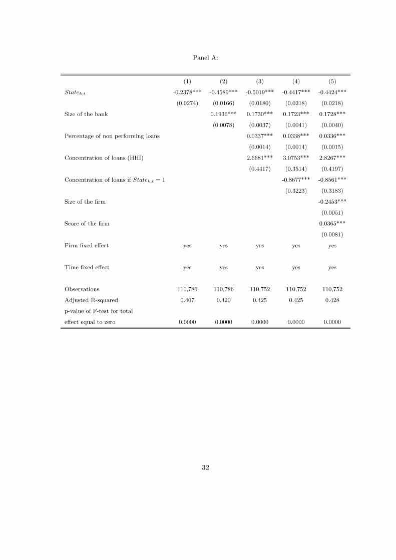
Panel A:

(1) (2) (3) (4) (5)

Statek,t -0.2378*** -0.4589*** -0.5019*** -0.4417*** -0.4424***

(0.0274) (0.0166) (0.0180) (0.0218) (0.0218)

Size of the bank 0.1936*** 0.1730*** 0.1723*** 0.1728***

(0.0078) (0.0037) (0.0041) (0.0040)

Percentage of non performing loans 0.0337*** 0.0338*** 0.0336***

(0.0014) (0.0014) (0.0015)

Concentration of loans (HHI) 2.6681*** 3.0753*** 2.8267***

(0.4417) (0.3514) (0.4197)

Concentration of loans if Statek,t = 1 -0.8677*** -0.8561***

(0.3223) (0.3183)

Size of the firm -0.2453***

(0.0051)

Score of the firm 0.0365***

(0.0081)

Firm fixed effect yes yes yes yes yes

Time fixed effect yes yes yes yes yes

Observations 110,786 110,786 110,752 110,752 110,752

Adjusted R-squared 0.407 0.420 0.425 0.425 0.428

p-value of F-test for total

effect equal to zero 0.0000 0.0000 0.0000 0.0000 0.0000

32

Panel B:

(1) (2) (3) (4) (5)

Statek,t -0.2293*** -0.4510*** -0.4980*** -0.4374*** -0.4376***

(0.0261) (0.0185) (0.0168) (0.0221) (0.0220)

Size of the bank 0.1895*** 0.1694*** 0.1689*** 0.1691***

(0.0087) (0.0042) (0.0046) (0.0045)


(0.0014) (0.0014) (0.0014)


(0.4835) (0.4297) (0.4958)


(0.3341) (0.3322)


(0.0065)


(0.0077)



Observations 97,792 97,792 97,760 97,760 97,760




33

Panel C:

(1) (2) (3)

Statek,t -0.4402*** -0.4382*** -0.4373***

(0.0220) (0.0225) (0.0220)

Size of the bank 0.1690*** 0.1691*** 0.1691***

(0.0045) (0.0045) (0.0045)


(0.0014) (0.0014) (0.0014)


(0.4914) (0.4976) (0.4946)

Concentration of loans if the bank is state-owned -0.8838*** -0.8751*** -0.8672***

(0.3284) (0.3258) (0.3323)

Size of the firm -0.2646*** -0.2647*** -0.2649***

(0.0065) (0.0066) (0.0064)

Score of the firm 0.0335*** 0.0335*** 0.0334***

(0.0076) (0.0076) (0.0077)

Statek,t = 1 if the firm has more than 8% of credit line usage 0.0150

(0.0127)

Statek,t = 1 if the firm has more than 15% of credit line usage 0.0214

(0.0303)

Statek,t = 1 if the firm has more than 37% of credit line usage -0.0364

(0.0456)

Firm fixed effect yes yes yes

Time fixed effect yes yes yes

Observations 97760 97760 97760

Adjusted R-squared 0.427 0.427 0.427


effect equal to zero 0.0000 0.0000 0.0000

34

Table 5:

Differences in interest rates charged

by state-owned and privately owned banks

I define the interest rate as the ratio of the quarterly payment (interest plus fees) paid by the firm

to the bank to its quarterly average balance minus the prime rate. In the second column, the interest

rate refers to the subsample of companies borrowing from state-owned banks; in the third column, to

the companies borrowing from privately owned banks. The difference is the average difference between

the second column (interest rates charged by state-owned banks) and the third column (interest rates

charged by privately owned banks). North includes the following regions: Piedmont, Valle d’Aosta,

Lombardy, Trentino, Veneto, Friuli Venezia Giulia, Liguria, and Emilia Romagna. Center includes

Tuscany, Umbria, Marche, and Lazio. South includes Abruzzo Molise, Campania, Puglia, Basilicata,

Calabria, Sicily, and Sardinia. For the difference, I test statistical significance using the t-statistic with

reference to a mean of zero. ***indicates statistically significant at the 1-percent level, ** indicates

statistically significant at the 5-percent level.

Interest rate-prime: State-owned banks Privately owned banks Difference Obs..

Borrowers classified by geographical location:

North 3.03 3.22 -.18*** 38,786

Center 3.02 3.41 -.39*** 6,292

South 3.20 3.65 -.45*** 3,818

Borrowers classified by size:

First quintile in sales 3.70 3.86 -.16*** 9,780

Second quintile in sales 3.34 3.55 -.21*** 9,778

Third quintile in sales 3.12 3.36 -.24*** 9,780

Fourth quintile in sales 2.84 3.10 -.25*** 9,780

Fifth quintile in sales 2.23 2.51 -.28*** 9,778

All borrowers 3.05 3.27 -.23*** 48,896

35

Table 6:

Interest rates charged by state-owned and

privately owned banks in different areas



bank. North includes the following regions: Piedmont, Valle d’Aosta, Lombardy, Trentino, Veneto,

Friuli Venezia Giulia, Liguria, and Emilia Romagna. Center includes Tuscany, Umbria, Marche, and

Lazio. South includes Abruzzo Molise, Campania, Puglia, Basilicata, Calabria, Sicily, and Sardinia.

I measure the size of the bank by logarithm of total assets. The percentage of nonperforming loans is

the ratio of nonperforming loans over total loans. I measure market concentration at the province level

by the Herfindahl-Hirschman Index (HHI) on total banking lending. Size of the firm is the logarithm

of sales. All regressions include year and firm dummies. Heteroskedasticity robust standard errors

are in brackets. The standard errors are corrected for within-year clustering. The table also reports

the p-value of an F-test for the hypothesis that the joint effect of all the variables equals zero.

36

(1) (2) (3) (4) (5)

Statek,t -0.1806*** -0.4102*** -0.4490*** -0.4562*** -0.4566***

(0.0231) (0.0195) (0.0143) (0.0203) (0.0202)

State if firm is located in the South -0.2709*** -0.2370*** -0.3097*** -0.3132*** -0.3143***

(0.0401) (0.0683) (0.0365) (0.0370) (0.0365)

State if firm is located in the North -0.2137*** -0.1501*** -0.1814*** -0.1818*** -0.1815***

(0.0112) (0.0123) (0.0145) (0.0154) (0.0154)

Size of the bank 0.1870*** 0.1655*** 0.1655*** 0.1657***

(0.0097) (0.0058) (0.0057) (0.0056)


(0.0016) (0.0016) (0.0016)


(0.4705) (0.4473) (0.5120)

Concentration of loans if Statek,t = 1 0.1093 0.1200

(0.3012) (0.2977)


(0.0064)


(0.0076)



Observations 97,792 97,792 97,760 97,760 97,760




37

Table 7:

Interest rates charged by state-owned and

privately owned banks by firms’ size



bank. I measure the size of the bank by logarithm of total assets. The percentage of nonperforming

loans is the ratio of nonperforming loans over total loans. I measure market concentration at the

province level by the Herfindahl-Hirschman Index (HHI) on total banking lending. Size of the firm is

the logarithm of sales. All the regressions include year and firm dummies. Heteroskedasticity robust

standard errors are in brackets. The standard errors are corrected for within-year clustering. The

table also reports the p-value of an F-test for the hypothesis that the joint effect of all the variables

equals zero.

38

(1) (2) (3) (4) (5)

Statek,t -0.2965*** -0.5151*** -0.5703*** -0.4937*** -0.4792***

(0.0301) (0.0427) (0.0324) (0.0321) (0.0323)

Statek,t if firm in smallest size quintile 0.1906*** 0.1868*** 0.2006*** 0.2113*** 0.1582***

(0.0366) (0.0338) (0.0380) (0.0377) (0.0391)

Statek,t if firm in second size quintile 0.0933** 0.0899** 0.1038** 0.1104** 0.0859**

(0.0419) (0.0411) (0.0443) (0.0446) (0.0417)

Statek,t if firm in third size quintile 0.0466 0.0396 0.0483 0.0536 0.0359

(0.0431) (0.0398) (0.0412) (0.0413) (0.0401)

Statek,t if firm in fourth size quintile 0.0287 0.0272 0.0320 0.0356 0.0258

(0.0253) (0.0231) (0.0241) (0.0242) (0.0237)

Size of the bank 0.1894*** 0.1692*** 0.1684*** 0.1688***

(0.0085) (0.0040) (0.0044) (0.0043)


(0.0013) (0.0013) (0.0013)


(0.4919) (0.4608) (0.5301)


(0.3375) (0.3233)


(0.0078)


(0.0076)



Observations 97,792 97,792 97,760 97,760 97,760


39

Table 8:

Electoral results, party affiliation and

interest rates charged by state-owned banks


rate at time t. I measure the local political strength of the party by the percentage of votes received

by the party to which the chairperson of the state-owned bank is affiliated in the area where the firm

is borrowing. I measure the size of the bank by logarithm of total assets. The percentage of non-

performing loans is the ratio of non-performing loans over total loans. I measure market concentration

at the province level by the Herfindahl-Hirschman Index (HHI) on total banking lending. Size of the

firm is the logarithm of sales. All the regressions include year and firm dummies. Heteroskedasticity

robust standard errors are in brackets. The standard errors are corrected for within-year clustering.

The table also reports the p-value of an F-test for the hypothesis that the joint effect of all the

variables equals zero. Column 1 sample includes all the observations (state-owned-banks-firm-year)

for which political affiliation of the president of the state-owned bank is available. Column 2 is the

same sample, excluding years 1994 and 1995. Columns 3 and 4 include only loans from national

state-owned banks.

40

(1) (2) (3) (4)

Local political strength of the party -0.2001** -0.2295*** -0.3240*** -0.2837***

(0.0806) (0.0844) (0.1239) (0.1005)

Size of the bank 0.1702*** 0.1641*** 0.1282***

(0.0065) (0.0033) (0.0237)


(0.0045) (0.0030) (0.0061)

Concentration of loans (HHI) 7.3368*** 8.0807*** 7.9113*** 7.7236***

(1.2113) (0.7930) (0.7298) (0.7004)

Size of the firm -0.3744*** -0.3277*** -0.3432*** -0.3435***

(0.0742) (0.0690) (0.0853) (0.0849)

Score of the firm 0.0321*** 0.0328** 0.0258 0.0258

(0.0087) (0.0144) (0.0167) (0.0167)

Time fixed effect yes yes yes yes

Firm fixed effect yes yes yes yes

Bank fixed effect no no no yes

Observations 26698 25049 17671 17671

Adjusted R-squared 0.4881 0.4953 0.5088 0.5087

41

References

Alesina, Alberto, Stephan Danninger, and Massimo V. Rostagno 1999, “Redistri-

bution through Public Employment: The Case of Italy”, NBER WP 6746,

Altman, Edward I., 1968, “Financial Ratios, Discriminant Analysis and the Prediction of Cor-

porate Bankruptcy”, Journal of Finance, 23: 589-609.

Altman, Edward I., 1993, Corporate financial distress and bankruptcy, John Wiley and Sons,

New York.

Altman, Edward I., Marco Giancarlo, and Varetto Franco, 1994, “Corporate dis-

tress diagnosis: Comparisons using linear discriminant analysis and neural networks (the Italian

experience)”, Journal of Banking and Finance, 18: 505-529.

Atkinson, A. B., and Joseph E. Stiglitz, 1980, Lectures on Public Economics, London, Mc-

Graw Hill..

Banerjee, Abhijit 1997, “A Theory of Misgovernance”, Quarterly Journal of Economics, 112:

1289-1332.

Barca, Fabrizio and Sandro Trento, 1996, “State-ownership and the evolution of Italian

corporate governance”, mimeo.

Barth, James R., Gerard Caprio, Jr. and Ross Levine, 2000, “Banking Systems Around

the Globe: Do Regulation and Ownership Affect Performance and Stability? ”, Working Paper

2325, World Bank.

Berger, Allen N., and Timothy H. Hannan, 1989, “The Price-Concentration Relationship

in Banking”, Review of Economics and Statistics, 71: 291-99.

De Bonis, Riccardo, 1998, “Public sector banks in Italy: past and present”, mimeo.

Detragiache, Enrica, Paolo G. Garella, and Luigi Guiso, 2000, “Multiple versus Sin-

gle Banking Relationship”, Journal of Finance, 55: 1133-1161.

42

Golden, Miriam, 2001, “The Effects of the Personal Vote on Political Patronage, Bureaucracy

and Legislation in Postwar Italy ”, working paper, Department of Political Science, UCLA.

Ginsborg, Paul, 1990, A history of contemporary Italy: society and politics, 1943-1988, Penguin

Books, London.

Greenwald, Bruce, and Joseph E. Stiglitz, 1986, “Externalities in Economies with Im-

perfect Information and Incomplete Markets”, Quarterly Journal of Economics, 101: 229-64.

Hannan, Timothy H., 1997, “Market Share Inequality, the Number of Competitors, and the

HHI: An Examination of Bank Pricing”, Review of Industrial Organization 12: 23-35.

Hart, Oliver, Andrei Shleifer, and Robert Vishny 1997, “The Proper Scope of Gov-

ernment: Theory and an Application to Prisons”, Quarterly Journal of Economics, 112: 1127-

1162.

La Porta, Rafael, Florencio Lopez-de-Silanes, Andrei Shleifer and Robert Vishny,

2002, “Government ownership of banks”, Journal of Finance, 57(1):256-301.

Laffont, Jean-Jacques, 1993, “Comments on “Public versus Regulated Enterprise”, by Willig,

Proceedings of the World Bank Annual Conference on Economic Development, Washington D.C.

International Bank for Reconstruction and Development/World Bank., 175-178

Laffont, Jean-Jacques and Jean Tirole, 1993, A Theory of Incentives in Regulation and

Procurement, MIT Press, Cambridge, MA.

Lopez-de-Silanes, Florencio, Andrei Shleifer and Robert Vishny, 1997, “Privati-

zation in the United States”, Rand Journal of Economics, 28(3):447-471.

Martiny, Mario, and Carmelo Salleo, 1997, “The Efficiency of Italian Banks: Some Em-

pirical Evidence”, mimeo.

Mayer, Colin, 2000, “Financial Systems, Corporate Finance, and Economic Development”, in

R.G. Hubbard (ed.) Asymmetric Information, Corporate Finance and Investment (pp.307-

332). Chicago:University of Chicago Press.

43

Pagano, Marco, Fabio Panetta, and Luigi Zingales, 1998, “Why Do Companies Go Pub-

lic? An Empirical Analysis”, Journal of Finance, 53: 27-64.

Rajan, Raghuram and Luigi Zingales, 1998, “Financial Dependence and Growth”, Ameri-

can Economic Review, 88(3): 559-586.

Sapienza, Paola, 2002, “The Effect of Banking Mergers on Loan Contracts”, Journal of Finance,

57(1):329-368

Shleifer, Andrei, 1998, “State versus Private Ownership”, Journal of Economic Perspectives.

Shleifer, Andrei and Robert W. Vishny, 1994, “Politicians and Firms”, Quarterly Jour-

nal of Economics, 109: 995-1025.

Shleifer, Andrei and Robert W. Vishny, 1998, The Grabbing Hand: Government Patholo-

gies and Their Cures, Harvard University Press, Cambridge, MA.

Stiglitz, Joseph E., 1993, “The role of the state in Financial Markets”, Proceedings of the World

Bank Annual Conference on Economic Development, Washington D.C. International Bank for

Reconstruction and Development/World Bank, pp. 19-56.

Stiglitz, Joseph E., and Andrew Weiss, 1981, “Credit Rationing in Markets with Imper-

fect Information”, American Economic Review, 71: 393-410.

Tirole, Jean, 1989, The Theory of Industrial Organization, The MIT Press, Cambridge, Mas-

sachusetts.

Tirole, Jean, 1994, “The Internal Organization of Governments”, Oxford Economic Papers, 46:

1-29.

Visentini, Gustavo, 2000, “Mixed and Market Oriented Economies: the Italian Situation”,

Mimeo, Universita’ Luiss Guido Carli, Rome, Italy.

44

Appendix I

Diagnostic System

The company data contain a numerical score for the firms in the sample that describes the

risk profile of the firm following Altman (1968, 1993). Both state- and privately owned banks had

access to the numerical score at the time when they lent to the firms. The score was obtained

by CB using two discriminant functions. This score express the “risk profile” of the business. A

detailed description of the methodology used by CB to calculate the numerical score is in Altman

et al. (1994). I used the score to classify the companies into seven zones: high security, security,

vulnerability, high vulnerability, uncertainty between vulnerability and risk, risk of bankruptcy; and

high risk of bankruptcy. The table below describe the risk profile of the companies contained in my

sample borrowing from state- and privately owned banks. By construction, the risk profile is identical

in the two sub-samples, thus only one table is included.

Table A.1.

SCORE Frequency Percent Cumulative Frequency

High security 1,420 2.6 1,420

Security 15,262 27.6 16,682

Vulnerability 409 .7 17,091

High vulnerability 11,743 21.2 28,834

Uncertainty between vulnerability and risk 13,471 24.3 42,305

Risk of bankruptcy 10,472 18.9 52,777

High risk of bankruptcy 2,616 4.7 55,393

45

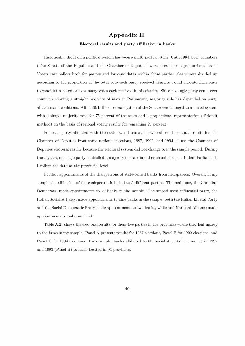
Appendix II

Electoral results and party affiliation in banks

Historically, the Italian political system has been a multi-party system. Until 1994, both chambers

(The Senate of the Republic and the Chamber of Deputies) were elected on a proportional basis.

Voters cast ballots both for parties and for candidates within those parties. Seats were divided up

according to the proportion of the total vote each party received. Parties would allocate their seats

to candidates based on how many votes each received in his district. Since no single party could ever

count on winning a straight majority of seats in Parliament, majority rule has depended on party

alliances and coalitions. After 1994, the electoral system of the Senate was changed to a mixed system

with a simple majority vote for 75 percent of the seats and a proportional representation (d’Hondt

method) on the basis of regional voting results for remaining 25 percent.

For each party affiliated with the state-owned banks, I have collected electoral results for the

Chamber of Deputies from three national elections, 1987, 1992, and 1994. I use the Chamber of

Deputies electoral results because the electoral system did not change over the sample period. During

those years, no single party controlled a majority of seats in either chamber of the Italian Parliament.

I collect the data at the provincial level.

I collect appointments of the chairpersons of state-owned banks from newspapers. Overall, in my

sample the affiliation of the chairperson is linked to 5 different parties. The main one, the Christian

Democrats, made appointments to 29 banks in the sample. The second most influential party, the

Italian Socialist Party, made appointments to nine banks in the sample, both the Italian Liberal Party

and the Social Democratic Party made appointments to two banks, while and National Alliance made

appointments to only one bank.

Table A.2. shows the electoral results for these five parties in the provinces where they lent money

to the firms in my sample. Panel A presents results for 1987 elections, Panel B for 1992 elections, and

Panel C for 1994 elections. For example, banks affiliated to the socialist party lent money in 1992

and 1993 (Panel B) to firms located in 91 provinces.

46

Table A.2.

A: 1987 election

mean sd min max Number of provinces

Christian Democrats .34565932 .08607512 .08375919 .52429986 80

Socialist Party .13883011 .028753 .06012196 .20933744 89

Italian Liberal Party .02274278 .01556027 .00539812 .09755591 52

Social Democratic Party .02849019 .01601734 .00475035 .09887846 71

B: 1992 election


Christian Democrats .30600768 .09383184 .07377624 .51638401 89

Socialist Party .13649238 .03488646 .04451371 .26654419 91

Italian Liberal Party .02806362 .01906862 .01006228 .13501064 70

Social Democratic Party .02611314 .01770669 .00560963 .07984234 76

C: 1994 election


Socialist Party .0183175 .0066557 .0094487 .0324773 33

National Alliance .1293044 .0635202 .0404381 .2955712 66

47

Documents

The Eï¬€ects of Government Ownership on Bank Lending