The E!ect of Knotting on the Shape of Polymers

Eric J. Rawdon! John C. Kern† Michael Piatek‡

Patrick Plunkett§ Andrzej Stasiak¶ Kenneth C. Millett"

August 13, 2008

Abstract

Momentary configurations of long polymers at thermal equilibriumusually deviate from spherical symmetry and can be better described, onaverage, by a prolate ellipsoid. The asphericity and nature of aspheric-ity (or prolateness) that describe these momentary ellipsoidal shapes of apolymer are determined by specific expressions involving the three princi-pal moments of inertia calculated for configurations of the polymer. Ear-lier theoretical studies and numerical simulations have established that asthe length of the polymer increases, the average shape for the statisticalensemble of random configurations asymptotically approaches a charac-teristic universal shape that depends on the solvent quality. It has beenestablished, however, that these universal shapes di!er for linear, circular,and branched chains. We investigate here the e!ect of knotting on theshape of cyclic polymers modeled as random isosegmental polygons. Weobserve that random polygons forming di!erent knot types reach asymp-totic shapes that are distinct from the ensemble average shape. For thesame chain length, more complex knots are, on average, more sphericalthan less complex knots.

1 Introduction

Ring polymer chains can be modeled as freely jointed random polygons. Thissimple representation of polymeric chains reflects their statistical properties

!Department of Mathematics, University of St. Thomas, St. Paul, MN 55105, USA,ejrawdon@stthomas.edu

†Department of Mathematics and Computer Science, Duquesne University, Pittsburgh, PA15282, USA, kern@mathcs.duq.edu

‡Department of Computer Science and Engineering, University of Washington, Seattle,WA 98195, USA, piatek@cs.washington.edu

§Department of Mathematics, University of California, Santa Barbara, Santa Barbara, CA93106, USA, plunkett@math.ucsb.edu

¶Faculty of Biology and Medicine, Center for Integrative Genomics, University of Lausanne,Lausanne CH 1015, Switzerland, corresponding author: Andrzej.Stasiak@unil.ch

"Department of Mathematics, University of California, Santa Barbara, Santa Barbara, CA93106, USA, millett@math.ucsb.edu

1

under the so-called !-conditions, where independent segments of the polymerchains neither attract nor repel each other.1 Under !!conditions, linear poly-mers behave like ideal random walks and show scaling exponent " = 0.5. Ifpolymer chains are circular the situation gets more complex as the scaling be-havior depends on whether one studies all possible configurations or just thosethat represent a given topological type like unknotted circles.2–11

It is an accepted convention in studies of shape and size of polymer chainsto characterize actual configurations adopted by the polymers by calculatingtheir inertial properties. Radius of gyration, i.e. the root mean square distancefrom the center of mass, is a standard measure of polymer size. In simulationstudies, the mass of the polymer is assumed to be equally distributed amongthe vertex points of the simulated chains. Studies of overall polymer size revealthat the radius of gyration of circular polymers for a fixed knot type scaleslike that of self-avoiding walks2–4,12,13 with an estimated scaling exponent " =0.5874±0.000214 while phantom polymers behave like neutral ideal chains withthe scaling exponent " = 0.5.

Studies of shapes of polymer chains use the three principal moments of inertiacalculated for given configuration of the chain to build an ellipsoid with thesame ratio of its principal moments of inertia as those of the given polymerconfiguration. Kuhn15 was first to propose that the overall shape of random coilsformed by polymer chains at thermodynamic equilibrium should, for entropicreasons, have the shape of a prolate ellipsoid. His proposal has been confirmedin numerical simulation studies (see e.g. Refs.9,16,17) and also in experimentalmeasurements.18,19 In the present study, we address how the shape and overallsize of polymer chains are influenced by the presence of knots in these polymers.

The ellipsoid of inertia is defined using the moment of inertia tensor,

Tij =1

2N2

N!

n=1

N!

m=1

(Xin ! Xi

m) · (Xjn ! Xj

m) (i = 1, 2, 3; j = 1, 2, 3), (1)

where Xin denotes the ith coordinate of the nth vertex and N is the number

of vertices in the polygon on which one has equally distributed the mass ofthe polymer. As Tij is a real symmetric tensor, it has three real eigenvalues#1, #2, #3 giving the three principal moments of inertia and determining thecorresponding eigenvectors providing the principal axes of inertia. The squareroots of #1, #2, #3 define the semi-axis lengths of the associated ellipsoid ofinertia.

A critical question is how to best measure the spatial extent of this ellip-soid. To accomplish this objective, in 1986 Aronovitz and Nelson20 proposed athree dimensional system, later modified by Cannon, Aronovitz and Goldbart,21

which separates the size calculation (measured by the squared radius of gyration,see Eqn. (4), which we will denote by R) from two shape descriptors: aspheric-ity, A, see Eqn. (2), and nature of asphericity, see Eqn. (3). In this definition,the asphericity and nature of asphericity are calculated using the three princi-pal moments of inertia, i.e. the eigenvalues #1, #2, #3 of Tij . The asphericitywas defined at the same time by Rudnick and Gaspari22 and has since become

2

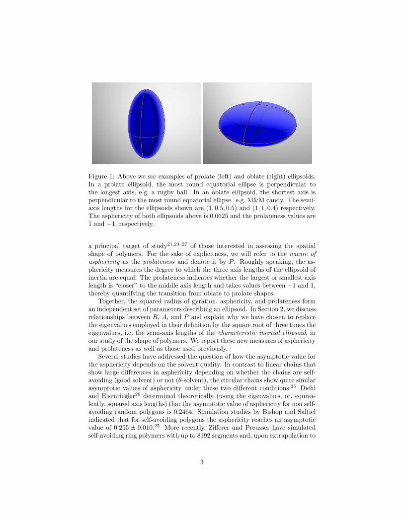
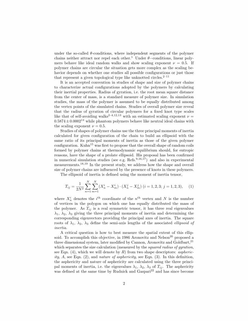
Figure 1: Above we see examples of prolate (left) and oblate (right) ellipsoids.In a prolate ellipsoid, the most round equatorial ellipse is perpendicular tothe longest axis, e.g. a rugby ball. In an oblate ellipsoid, the shortest axis isperpendicular to the most round equatorial ellipse. e.g. M&M candy. The semi-axis lengths for the ellipsoids shown are (1, 0.5, 0.5) and (1, 1, 0.4) respectively.The asphericity of both ellipsoids above is 0.0625 and the prolateness values are1 and !1, respectively.

a principal target of study21,23–27 of those interested in assessing the spatialshape of polymers. For the sake of explicitness, we will refer to the nature ofasphericity as the prolateness and denote it by P . Roughly speaking, the as-phericity measures the degree to which the three axis lengths of the ellipsoid ofinertia are equal. The prolateness indicates whether the largest or smallest axislength is “closer” to the middle axis length and takes values between !1 and 1,thereby quantifying the transition from oblate to prolate shapes.

Together, the squared radius of gyration, asphericity, and prolateness forman independent set of parameters describing an ellipsoid. In Section 2, we discussrelationships between R, A, and P and explain why we have chosen to replacethe eigenvalues employed in their definition by the square root of three times theeigenvalues, i.e. the semi-axis lengths of the characteristic inertial ellipsoid, inour study of the shape of polymers. We report these new measures of asphericityand prolateness as well as those used previously.

Several studies have addressed the question of how the asymptotic value forthe asphericity depends on the solvent quality. In contrast to linear chains thatshow large di!erences in asphericity depending on whether the chains are self-avoiding (good solvent) or not (!-solvent), the circular chains show quite similarasymptotic values of asphericity under these two di!erent conditions.25 Diehland Eisenriegler26 determined theoretically (using the eigenvalues, or, equiva-lently, squared axis lengths) that the asymptotic value of asphericity for non self-avoiding random polygons is 0.2464. Simulation studies by Bishop and Saltielindicated that for self-avoiding polygons the asphericity reaches an asymptoticvalue of 0.255 ± 0.010.25 More recently, Zi!erer and Preusser have simulatedself-avoiding ring polymers with up to 8192 segments and, upon extrapolation to

3

(a) R # 7.08A # 0.35P # 0.99

(b) R # 4.03A # 0.068P # 0.67

(c) R # 1.73A # 0.0012P # $0.52

Figure 2: Examples of 50 edge polygonal trefoil knots with high, medium, andlow asphericity shown with their characteristic inertial ellipsoids.

infinite chain length, concluded that the asymptotic value of asphericity for thissystem is 0.2551 ± 0.0005.16 One of the goals of this manuscript is to estimatenumerically this asymptotic value for polygons with a fixed knot type.

When a polygon has between three and five vertices, the only knot possibleis the unknot, i.e. a polygon that is topologically equivalent to a circle. Atsix edges, the first nontrivial knot appears, the trefoil knot, known as 31. Forincreasing numbers of edges, more and more di!erent (and more complicated)types of knots become possible (see e.g. Refs.28–30 for a discussion of the minimalnumber of edges in an equilateral polygon required to realize each knot type andthe growth of the number of knot types possible as a function of the numberof edges). In addition, the probability of obtaining a knotted polymer tends toone as the length goes to infinity.31–34

Here we investigate the shape of circular polymers with fixed knot type, asmeasured by their asphericity and prolateness, and determine the dependenceof shape on the length and knotting of the polymer. We find that for “small”numbers of edges, polymers of a fixed nontrivial knot type tend to be morespherical (lower asphericity) than phantom polygons with the same number ofedges. However the opposite is true for very long knotted chains that, at least incase of the knot types we analyzed, become less spherical than phantom polygons(see Figs. 6 and 8). Prolateness shows a more complex behavior: short knottedchains of a given nontrivial knot type are initially less prolate than phantompolygons of the same size. Then, in the intermediate size range, the knottedchains become more prolate than the corresponding phantom chains. Finally, inthe long chain regime, we again observe that knotted chains become less prolatethan phantom chains (see Figs. 7 and 8).

2 Exploration of Shape Measures

As discussed in the previous section, we use a slight variation on asphericityand prolateness to measure the shape of individual ellipsoids describing circular

4

polymers as we replace the principal moments of inertia, i.e. eigenvalues of themoment of inertia tensor, by the square root of three times the eigenvalues. Toexplain why this is helpful we first review the principal concepts: the asphericityis a number between 0 (implying a spherical shape when a = b = c) and 1(implying a rod-like shape when b = c = 0) and is defined by

A(a, b, c) =(a ! b)2 + (a ! c)2 + (b ! c)2

2(a + b + c)2(2)

where a, b, and c are measurements of the size of the ellipsoid of inertia. Theprolateness has values between !1 (oblate, e.g. when a = b > c) and 1 (prolate,e.g. when a > b = c) and is defined by

P (a, b, c) =(2a ! b ! c)(2b ! a ! c)(2c ! a ! b)

2(a2 + b2 + c2 ! ab ! ac ! bc)3/2. (3)

To get a sense for the values of prolateness, assume that a " b " c " 0.Then P (a, b, c) = 0 when b = a+c

2 . When b < a+c2 , the prolateness is positive

(i.e. the ellipsoid is prolate) and when b > a+c2 , the prolateness is negative

(i.e. the ellipsoid is oblate). Note that both A and P are invariant of scale andsymmetric in a, b, and c.

As discussed earlier, traditionally the principal moments of inertia #1, #2,and #3 have been used as the arguments a, b, and c.20–27 The scaling argumentsused to predict asymptotic values for random walks, random polygons, starshapes, etc., use these eigenvalues as well. Cannon et al.21 observed that theasphericity is “biased towards larger configurations”. However, with additionalcare in the definitions, one can eliminate the bias of R in A while preserving theunbiased nature of P .

One of the goals in defining the asphericity and, subsequently, the nature ofasphericity or prolateness, is to have true measures of shape that are unbiasedby the size of the polygon. A standard measure of the size of a polymer, thesquared radius of gyration, is determined from its moment of inertia tensor asthe sum of its three eigenvalues:

R = #1 + #2 + #3 . (4)

With the objective of eliminating the scale bias, we first define an ellipsoidwhose principal moments of inertia and principal axes coincide with those of thepolygon. This ellipsoid has semi-axis lengths of $i =

#3#i, i = 1, 2, 3. We refer

to this ellipsoid as the characteristic inertial ellipsoid (see Fig. 2 where one canobserve the relationship between polygons and their associated characteristicinertial ellipsoids).

The characteristic inertial ellipsoid has the attractive property that the char-acteristic inertial ellipsoid of an ellipsoid is itself. This is consistent with thedefinition of the radius of gyration, for example, where a sphere of radius r hasradius of gyration equal to r. In contrast, the ellipsoid of inertia of an ellipsoidhas the same principal axes of inertia but the semi-axis lengths are scaled bythe factor 1

!

3, i.e. the ellipsoid of inertia is a shrunken version of the original.

5

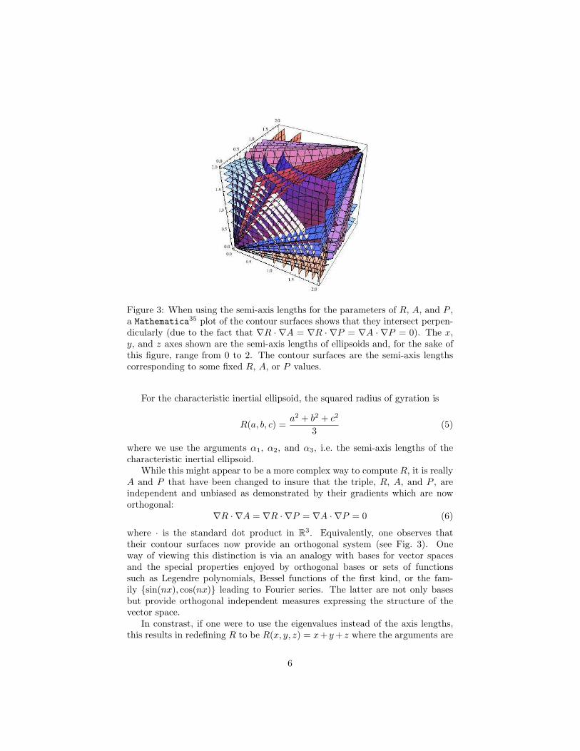
Figure 3: When using the semi-axis lengths for the parameters of R, A, and P ,a Mathematica

35 plot of the contour surfaces shows that they intersect perpen-dicularly (due to the fact that $R ·$A = $R ·$P = $A ·$P = 0). The x,y, and z axes shown are the semi-axis lengths of ellipsoids and, for the sake ofthis figure, range from 0 to 2. The contour surfaces are the semi-axis lengthscorresponding to some fixed R, A, or P values.

For the characteristic inertial ellipsoid, the squared radius of gyration is

R(a, b, c) =a2 + b2 + c2

3(5)

where we use the arguments $1, $2, and $3, i.e. the semi-axis lengths of thecharacteristic inertial ellipsoid.

While this might appear to be a more complex way to compute R, it is reallyA and P that have been changed to insure that the triple, R, A, and P , areindependent and unbiased as demonstrated by their gradients which are noworthogonal:

$R ·$A = $R ·$P = $A ·$P = 0 (6)

where · is the standard dot product in R3. Equivalently, one observes thattheir contour surfaces now provide an orthogonal system (see Fig. 3). Oneway of viewing this distinction is via an analogy with bases for vector spacesand the special properties enjoyed by orthogonal bases or sets of functionssuch as Legendre polynomials, Bessel functions of the first kind, or the fam-ily {sin(nx), cos(nx)} leading to Fourier series. The latter are not only basesbut provide orthogonal independent measures expressing the structure of thevector space.

In constrast, if one were to use the eigenvalues instead of the axis lengths,this results in redefining R to be R(x, y, z) = x+ y + z where the arguments are

6

now #1, #2, #3. The definitions of A and P remain the same. In such a case, we

still obtain $R·$P = $A·$P = 0. However, $R·$A = 6(xy+xz+yz"x2"y2

"z2)(x+y+z)3

thereby showing the inherent bias in the system.In order to employ unbiased measures of shape, we will use R, A, and P

with the semi-axis lengths of the characteristic inertial ellipsoid $1, $2, and$3 as arguments. As a consequence, the specific numerical results di!er fromprevious theoretical and numerical studies. However, we present both values inTable 1 and observe that our data provides estimates using the eigenvalues whichare consistent with those found in earlier studies. Note that due to the scaleinvariance of A and P (using either the eigenvalues or the semi-axis lengths)and the fact that the semi-axis lengths of ellipsoid of inertia and characteristicinertial ellipsoid di!er by a common factor of 1/

#3, the ellipsoid of inertia and

characteristic inertial ellipsoid share the same A and P values.The asphericity and prolateness, together, give a quantification of the shape

of the polymer (see Figs. 6, 7, and 8). The dominant factor is the asphericitywhich measures the degree to which the three eigenvalues of the inertial tensorare equal. For example, an ellipsoid with semi-axis lengths 1, 1, and 0.4 hasasphericity equal to 0.0625 and prolateness equal to !1. In contrast, with thesame asphericity of 0.0625, one has the other extreme, a prolate ellipsoid withone axis of length 1 and two axes of length 1/2, giving a prolateness equal to +1(see Fig. 1). When the asphericity is very close to zero, i.e. the semi-axis lengthsare almost equal, the variation between the most and least prolate shapes isextremely small as the shape is constrained by the asphericity. For example, anellipsoid with semi-axis lengths 1, 1, and 0.99 has A % 1.13& 10"5 and P = !1while an ellipsoid with semi-axis lengths 1, 0.99, 0.99 has A % 1.12 & 10"5 andP = 1.

Therefore, the asphericity provides a first-order measurement of the shape ofthe polymer, and prolateness is a second-order descriptor of how the asphericityvalue is attained. Note that for a given asphericity value, not all prolatenessvalues are possible. For example, a rod-like shape has asphericity close to 1thereby forcing the prolateness to take values close to 1 as well. In fact, aprolateness of !1 is possible only with shapes where A ' 1/4.

3 Computations

We have analyzed equilateral random polygons from 6 to 48 edges with a stepsize of 2 and from 50 edges to 500 edges by a step size of 10 edges. For each num-ber of edges, we generated 400,000 random knots using the hedgehog method.36

To identify the knot type of each of the polygons, we calculated the HOMFLYpolynomial37 using the program of Ewing and Millett.38 As the HOMFLY poly-nomial is not faithful to the knot type (i.e. there exist knots which are distinctbut which have the same HOMFLY polynomial), we actually determine the dis-tribution of HOMFLY polynomials of the random polygons and employ this asa surrogate for the knot type. However, the probability of finding other knotswith the same HOMFLY polynomials as the simple knot types analyzed here

7

is orders of magnitude lower than the probability of these simple knot types.Therefore, Fig. 5 gives a faithful presentation of the probabilities of knots stud-ied here. This set of random knots was also used in10,11 and a more detaileddescription of the generation method can be found there.

We calculate the asphericity and prolateness for each of the random knotsand keep a running list of the asphericity and prolateness values for the givenHOMFLY polynomial with the given number of edges. Average asphericity andprolateness values are then computed for the knots 01, 31, 41, 51, 52, 61, 62, and63 and for the entire knot population (i.e. phantom polygons) at each numberof edges. Because the average asphericity and prolateness for the two versionsof chiral knots will be the same, we combine those data sets. For example, +31

and !31, the right and left handed versions of the trefoil knot, are combinedinto a common 31 file to provide more robust data. The other chiral knots inthis study are 51, 52, 61, and 62.

One of the goals of this research is to describe the asymptotic shape of knot-ted and phantom polygons. To this end, we have estimated the asymptoticvalues of the asphericity, for both the axis length and the eigenvalue definitions,for the di!erent classes of polygons. We used a Monte Carlo Markov Chainanalysis, described in more detail in Ref.11 and its Supporting Information, tocompute 95% confidence intervals for the asymptotic value. The fitting func-tion27 A + B/

#x + C/x is used and applied to the data for 100 edges and

larger, wishing to minimize small edge e!ects. For a fixed number of edges, theasphericity values are not normally distributed for a given knot type nor forthe phantom polygons, so the grouping procedure described in Ref.11 was used.Gibbs Sampling39 was utilized to minimize computation time. In the end, wecomputed approximately 3500 likely fitting functions for the phantom polygonsand each of the knot types. The values shown in Table 1 correspond to the meanand 95% confidence ranges for the value of A in the likely fitting functions.

4 Asphericity and prolateness of knotted poly-

mers

The random polygons were divided into the individual knot types and theirshapes were analyzed in terms of asphericity and prolateness. Figures 6, 7, and8 show how the average asphericity and prolateness depend on the knot typeand the size of the polygon. It is interesting to analyze some of these profiles inorder to understand better their meaning. The asphericity profile for unknots(see Fig. 6) shows that for small number of segments (say 6 and 8 segments),the unknotted polygons deviate strongly from spherical symmetry. However,the asphericity values in this range do not tell us whether the polygons areaspherical due to adopting discoidal planar configurations or due to formingvery elongated shapes. Inspection of Fig. 7 reveals, however, that unknottedpolygons with 6 or 8 segments have on average positive prolateness. Therefore,we can conclude that the dominant deviation from spherical symmetry for un-

8

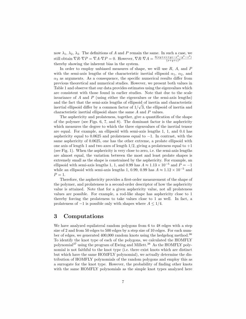
Figure 4: A hexagonal equilateral 31 is shown with A % 0.05 and P % !0.3, themean values for 6-edge trefoils. Because the minimum number of edges requiredto construct a trefoil is 6, the configurations tend to be nearly planar, forcingthe characteristic inertial ellipsoid to be oblate. The thickened polygon andellipsoid are shown from a position slightly o! the longest principal axis.

knotted polygons with small number of segments is towards forming elongatedconfigurations. This contrasts with the negative prolateness of polygons with6 segments that form trefoil knots (see Fig. 7) and have on average an oblateshape (negative prolateness). In fact, isosegmental hexagons forming trefoilknots are quite restricted in their freedom to change shapes and adopt ratherregular planar configurations. Figure 4 shows a hexagonal trefoil with a typicalshape (A % 0.05, P % !0.3) together with its characteristic inertial ellipsoid.However, polygons forming trefoil knots with increasing number of segmentsquickly become prolate on average (see Fig. 7) and their asphericity increases(see Fig. 6).

A more general comparison of the asphericity of polygons forming di!erentknot types reveals that for a given number of segments, the polygons formingmore complex knots are on average more spherical, i.e. have lower asphericity,than polygons forming less complex knots (see Fig. 6). We expect howeverthat for very long polymers the asphericity values of various simple knots willapproach the same universal value. A general comparison of prolateness ofpolygons forming various knot types (see Fig. 7) reveals that for a given numberof segments, the prolateness of less complex knots is lower than that of morecomplex knots. It is interesting to note that for the individual knot typesanalyzed here, the prolateness reaches its maximal value for relatively shortpolygons (n < 70) and then shows a decrease. It may seem contradictory thatthe decrease in prolateness with the increasing chain length is associated withincreasing asphericity (compare Figs. 6, 7, and 8). However, there is no realcontradiction as the flattening of a rugby ball shape from its sides decreases itsprolateness and increases its asphericity.

After exploring the asphericity and prolateness profiles for polygons formingindividual knot types, let us analyze the corresponding profiles for the ensemble

9

average of all polygons grouped together. Such a statistical set represents phan-tom polygons that can freely undergo intersegmental passages such as thoseexemplified by circular DNA molecules in the presence of type II DNA topoiso-merase. Of course, the profile of all polygons is the weighted average of profilesfor individual knot types where the relative probability of a given knot typeis taken into account. Therefore, for very small number of segments, whereunknots dominate, the profile for phantom polygons closely follows that of theunknots. As polygon sizes increase and nontrivial knots become frequent, theasphericity and prolateness of phantom polygons rapidly approach their respec-tive characteristic constant values.

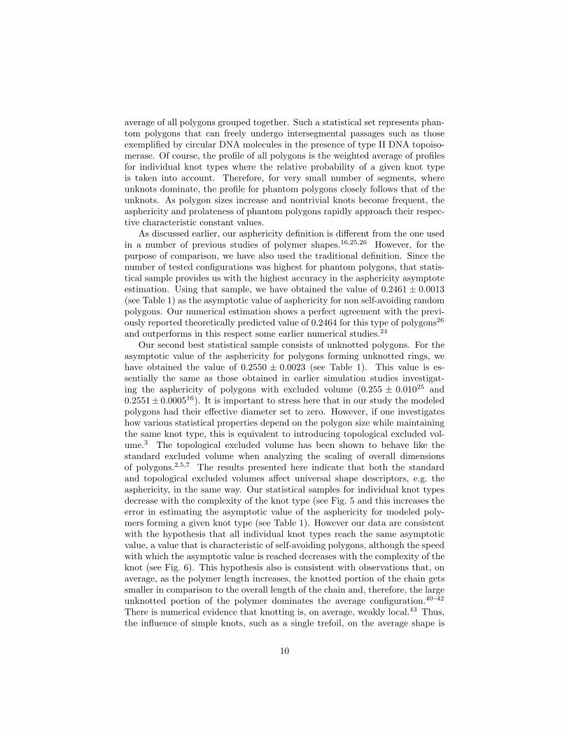
As discussed earlier, our asphericity definition is di!erent from the one usedin a number of previous studies of polymer shapes.16,25,26 However, for thepurpose of comparison, we have also used the traditional definition. Since thenumber of tested configurations was highest for phantom polygons, that statis-tical sample provides us with the highest accuracy in the asphericity asymptoteestimation. Using that sample, we have obtained the value of 0.2461 ± 0.0013(see Table 1) as the asymptotic value of asphericity for non self-avoiding randompolygons. Our numerical estimation shows a perfect agreement with the previ-ously reported theoretically predicted value of 0.2464 for this type of polygons26

and outperforms in this respect some earlier numerical studies.24

Our second best statistical sample consists of unknotted polygons. For theasymptotic value of the asphericity for polygons forming unknotted rings, wehave obtained the value of 0.2550 ± 0.0023 (see Table 1). This value is es-sentially the same as those obtained in earlier simulation studies investigat-ing the asphericity of polygons with excluded volume (0.255 ± 0.01025 and0.2551± 0.000516). It is important to stress here that in our study the modeledpolygons had their e!ective diameter set to zero. However, if one investigateshow various statistical properties depend on the polygon size while maintainingthe same knot type, this is equivalent to introducing topological excluded vol-ume.3 The topological excluded volume has been shown to behave like thestandard excluded volume when analyzing the scaling of overall dimensionsof polygons.2,5,7 The results presented here indicate that both the standardand topological excluded volumes a!ect universal shape descriptors, e.g. theasphericity, in the same way. Our statistical samples for individual knot typesdecrease with the complexity of the knot type (see Fig. 5 and this increases theerror in estimating the asymptotic value of the asphericity for modeled poly-mers forming a given knot type (see Table 1). However our data are consistentwith the hypothesis that all individual knot types reach the same asymptoticvalue, a value that is characteristic of self-avoiding polygons, although the speedwith which the asymptotic value is reached decreases with the complexity of theknot (see Fig. 6). This hypothesis also is consistent with observations that, onaverage, as the polymer length increases, the knotted portion of the chain getssmaller in comparison to the overall length of the chain and, therefore, the largeunknotted portion of the polymer dominates the average configuration.40–42

There is numerical evidence that knotting is, on average, weakly local.43 Thus,the influence of simple knots, such as a single trefoil, on the average shape is

10

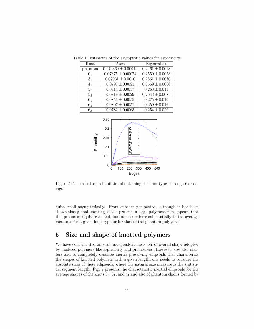
Table 1: Estimates of the asymptotic values for asphericity.

Knot Axes Eigenvaluesphantom 0.074360 ± 0.00042 0.2461 ± 0.0013

01 0.07875 ± 0.00074 0.2550 ± 0.002331 0.07931 ± 0.0010 0.2561 ± 0.003041 0.0797 ± 0.0021 0.2569 ± 0.006651 0.0814 ± 0.0037 0.263 ± 0.01152 0.0819 ± 0.0029 0.2643 ± 0.008561 0.0853 ± 0.0055 0.275 ± 0.01662 0.0807 ± 0.0051 0.259 ± 0.01663 0.0782 ± 0.0063 0.254 ± 0.020

0

0.05

0.1

0.15

0.2

0.25

0 100 200 300 400 500

Prob

abilit

y

Edges

0131415152616263

Figure 5: The relative probabilities of obtaining the knot types through 6 cross-ings.

quite small asymptotically. From another perspective, although it has beenshown that global knotting is also present in large polymers,44 it appears thatthis presence is quite rare and does not contribute substantially to the averagemeasures for a given knot type or for that of the phantom polygons.

5 Size and shape of knotted polymers

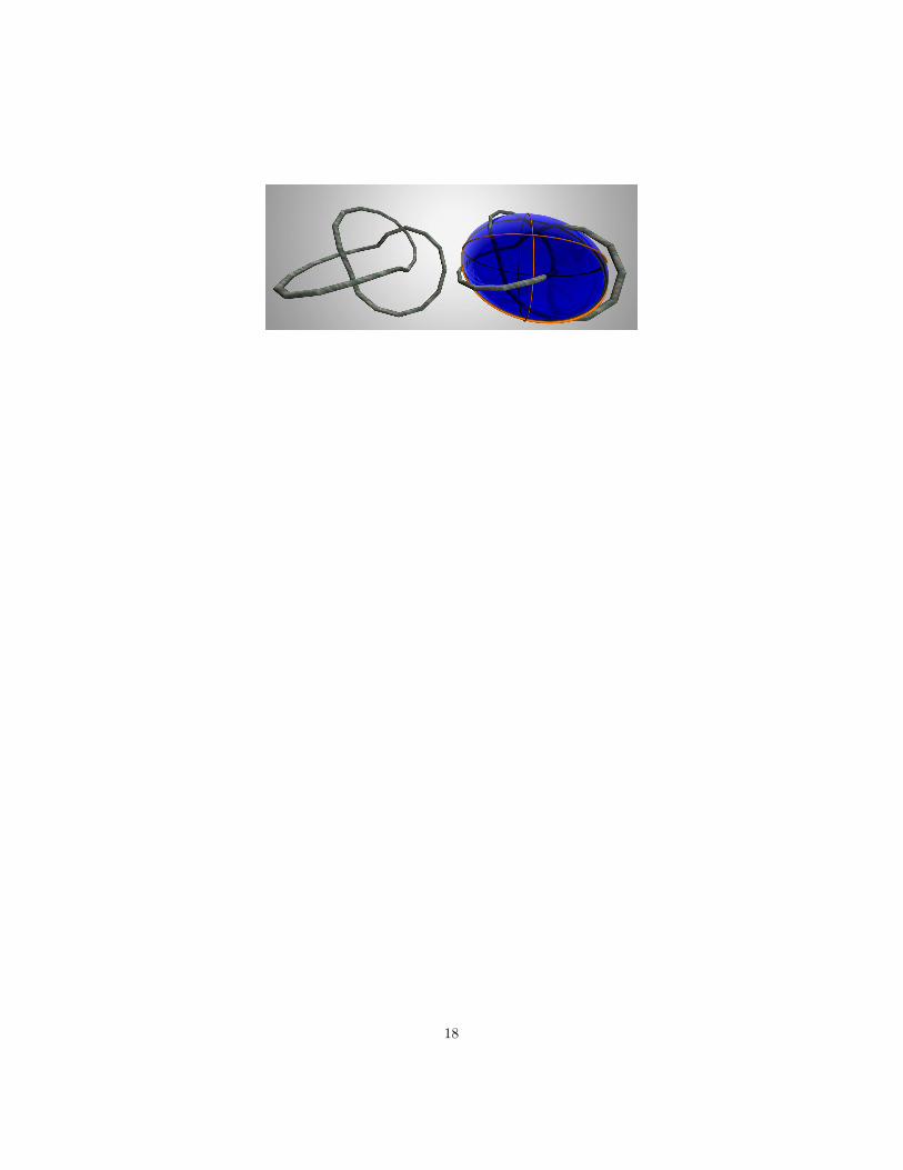
We have concentrated on scale independent measures of overall shape adoptedby modeled polymers like asphericity and prolateness. However, size also mat-ters and to completely describe inertia preserving ellipsoids that characterizethe shapes of knotted polymers with a given length, one needs to consider theabsolute sizes of these ellipsoids, where the natural size measure is the statisti-cal segment length. Fig. 9 presents the characteristic inertial ellipsoids for theaverage shapes of the knots 01, 31, and 41 and also of phantom chains formed by

11

0.03

0.04

0.05

0.06

0.07

0.08

0.09

0.1

0 100 200 300 400 500

Asph

erici

ty

Edges

phantom01314151 0.068

0.069 0.07

0.071 0.072 0.073 0.074 0.075 0.076 0.077 0.078

0 100 200 300 400 500

Asph

erici

ty

Edges

phantom01314151

Figure 6: Scaling profiles for the average asphericity of knotted polygons andphantom polygons. In the right panel, we restrict the vertical dimension toshow the asymptotic nature of the graphs more clearly.

-0.4-0.3-0.2-0.1

0 0.1 0.2 0.3 0.4 0.5

0 100 200 300 400 500

Prol

aten

ess

Edges

phantom01314151 0.28

0.29 0.3

0.31 0.32 0.33 0.34 0.35 0.36 0.37

0 100 200 300 400 500

Prol

aten

ess

Edges

phantom01314151

Figure 7: Scaling profiles for the average prolateness of knotted polygons andphantom polygons. In the right panel, we restrict the vertical dimension toshow the asymptotic nature of the graphs more clearly.

12

-0.4-0.3-0.2-0.1

0 0.1 0.2 0.3 0.4

0.05 0.06 0.07 0.08 0.09

Prol

aten

ess

Asphericity

phantom013141

0.26

0.28

0.3

0.32

0.34

0.36

0.066 0.070 0.074 0.078

Pro

late

ne

ss

Asphericity

phantom013141

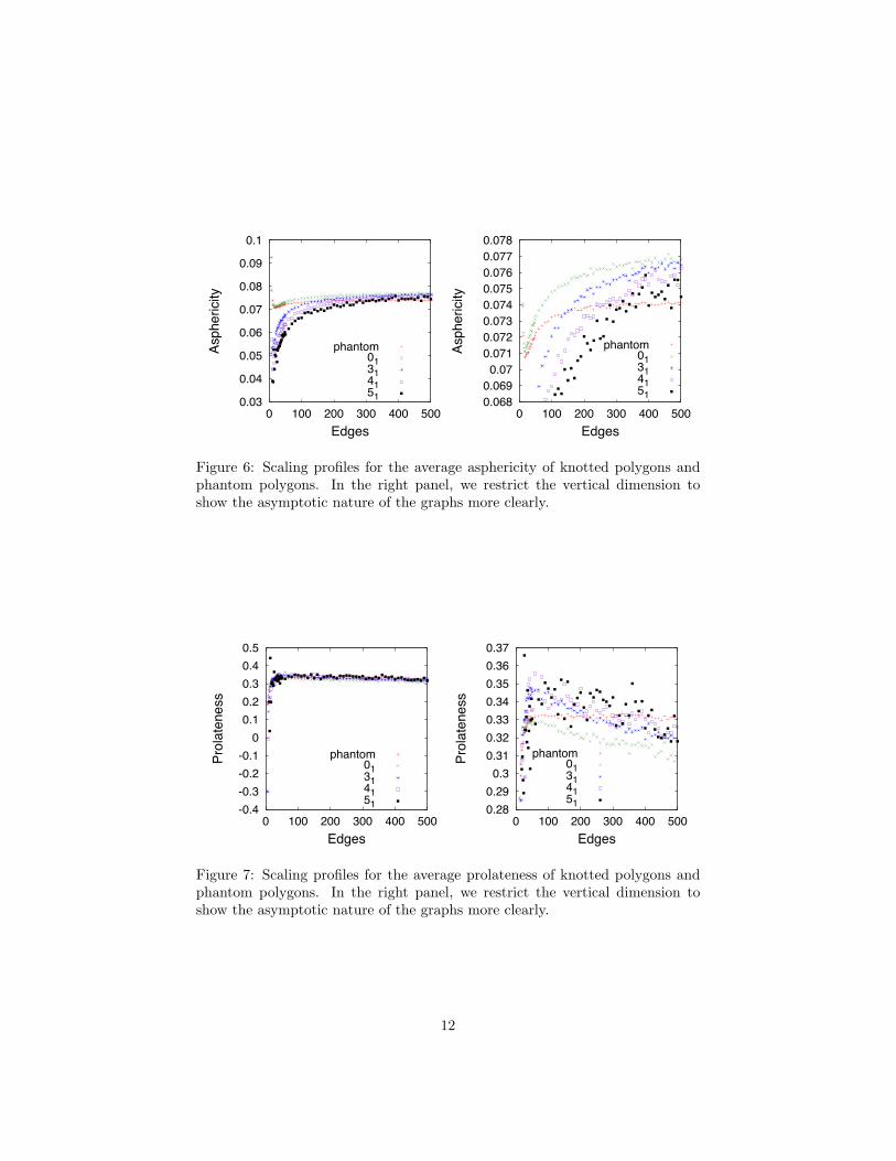
Figure 8: Average asphericity and prolateness for phantom polygons, 01, 31,and 41 knotted polymers with increasing length. The arrows show the directionof increasing numbers of edges. In the right panel, we restrict the verticaldimension to show the asymptotic nature of the graphs more clearly.

500 edge polygons. This form of presentation (nested ellipsoids) allows visualcomparison of average shapes of polygons with di!erent topology. We can seethat the ellipsoid characterizing unknots forms the external shell and thereforeis bigger than ellipsoids characterizing nontrivial knots. As the knots get morecomplicated, the ellipsoids representing them become smaller. However, theymaintain very similar aspect ratios and it is hardly visible that 41 knots are onaverage more spherical than unknots (see Fig. 6). The most internal shell inFig. 9 represents phantom polygons as these have the smallest overall dimen-sions from this set of knots. However, more complex knots, e.g. the 10165 knot,would be smaller than phantom knots for polygons with 500 edges.

The situation presented in Fig. 9 illustrates the particular case of 500 edgepolygons. What would be the corresponding image for very long chains? Weconjecture that for such a situation, the nested ellipsoids would be very closelyspaced, like onion skins. The external skin would be still that of the unknot,and the sequential skins would be ordered according to the complexity of theknot 31, 41, five crossing knots, six crossing knots, etc. Toward the center ofthe onion, one would have extremely complex knots, while the skin representingthe average size of phantom knots would be placed between the external skinrepresenting unknots and the internal skins representing most complex knotspossible for this size of the polygon. We also conjecture that the external skins(i.e. ellipsoids) representing simple prime knots would all be asymptoticallyclose to the aspect ratio attained by the ellipsoid representing unknots, whilevery complex knots would be more spherical. At this point, we are uncertainwhether the order of the skins for all knots will be the same for all chain sizes,i.e. whether there could be an example of two knot types where one would haveits overall dimensions smaller than the other at 500 segments, for example, but

13

Figure 9: Average ellipsoids for 500 edge 01 (in blue), 31 (in green), 41 (in red),and phantom polygons (in yellow) as seen along the two shortest axes of inertia.The black bar below the ellipsoids represents the size of 10 statistical segments.

not at 1000 segments. However, it is probably safe to conjecture that the orderof skins (ellipsoids) representing knots belonging to the same family of knots(like simple torus knots 31, 51, 71, etc.), will always follow the order of theminimal crossing number, provided that the number of segments in the polygonis significantly bigger than the minimal number of segments needed to formmost complex knots under consideration.

6 Conclusions

The notion that the overall shape of randomly fluctuating polymeric moleculescan be approximated by prolate ellipsoids rather than by spheres was publishedin 1934 by Kuhn.15 Over the years theoretical and numerical studies haveestablished that as the chain size tends to infinity, the asphericities of ellipsoidsdescribing the inertial properties of modeled polymers asymptotically approachcharacteristic constant values.9,16,17,20–22,24–26 These values are known to bedi!erent for linear and circular chains and are, in addition, influenced by thesolvent quality. Here we have provided unbiased measures of inertial shape andestablished that the topology of the chains also a!ects their overall shape. Wehave shown that for a fixed chain size, the modeled polymer molecules formingless complex knots are, on average, more spherical than configurations of morecomplex knotted chains. Furthermore, for each knot type, there is a chain lengthstarting with which polygons representing this knot type will be on average lessspherical than the average shape of phantom polygons for every number ofsegments beyond this length.

14

Acknowledgments

KCM, EJR, and AS wish to thank the Institute for Mathematics and its Appli-cations (Minneapolis, MN, USA, with funds provided by the National ScienceFoundation) for support during the thematic year: Mathematics of Molecu-lar and Cellular Biology. KCM also thanks the Centre de Mathematiques etd’Informatique (Marseille, France) for the hospitality during this work. AS wassupported in part by Swiss National Science Foundation grant 3100A0-116275.

References

1. de Gennes, P. G. Scaling Concepts in Polymer Physics; Cornell UniversityPress: Ithaca, N.Y., 1979.

2. Deutsch, J. M. Phys. Rev. E 1999, 59, 2539–2541.

3. Grosberg, A. Y. Phys. Rev. Lett. 2000, 85, 3858–3861.

4. Shimamura, M. K.; Deguchi, T. Physical Review E (Statistical, Nonlinear,and Soft Matter Physics) 2002, 65, 051802.

5. Dobay, A.; Dubochet, J.; Millett, K.; Sottas, P.-E.; Stasiak, A. Proc. Natl.Acad. Sci. USA 2003, 100, 5611–5615.

6. Diao, Y.; Dobay, A.; Kusner, R. B.; Millett, K. C.; Stasiak, A. J. Phys. A2003, 36, 11561–11574.

7. Moore, N. T.; Lua, R. C.; Grosberg, A. Y. Proc. Natl. Acad. Sci. USA 2004,101, 13431–13435.

8. Millett, K.; Dobay, A.; Stasiak, A. Macromolecules 2005, 38, 601–606.

9. Steinhauser, M. O. The Journal of Chemical Physics 2005, 122, 094901–1–13.

10. Plunkett, P.; Piatek, M.; Dobay, A.; Kern, J.; Millett, K.; Stasiak, A.;Rawdon, E. Macromolecules 2007, 40, 3860–3867.

11. Rawdon, E.; Dobay, A.; Kern, J. C.; Millett, K. C.; Piatek, M.; Plunkett, P.;Stasiak, A. Macromolecules 2008, 41, 4444–4451.

12. des Cloizeaux, J. J. Phys. Lett. (France) 1981, 42, L433–436.

13. Shimamura, M. K.; Deguchi, T. J. Phys. A 2002, 35, 241–246.

14. Prellberg, T. J. Phys. A: Math. Gen. 2001, 34, L599–L602.

15. Kuhn, W. Colloid & Polymer Science 1934, 68, 2–15.

16. Zi!erer, G.; Preusser, W. Macromol. Theory Simul. 2001, 10, 397–407.

15

17. Guo, L.; Luijten, E. Macromolecules 2003, 36, 8201–8204.

18. Haber, C.; Ruiz, S. A.; Wirtz, D. Proc. Natl. Acad. Sci. USA 2000, 97,10792–10795.

19. Maier, B.; Radler, J. O. Macromolecules 2001, 34, 5723–5724.

20. Aronovitz, J. A.; Nelson, D. R. J. Physique 1986, 47, 1445–1456.

21. Cannon, J. W.; Aronovitz, J. A.; Goldbart, P. J. Physique I 1991, 1, 629–645.

22. Rudnick, J.; Gaspari, G. J. Phys. A: Math. Gen. 1986, 19, L191–L193.

23. Theodorou, D. N.; Suter, U. W. Macromolecules 1985, 18, 1206–1214.

24. Bishop, M.; Michels, J. P. J. J. Chem. Phys. 1986, 85, 1074–1076.

25. Bishop, M.; Saltiel, C. J. J. Chem. Phys. 1988, 88, 3976–3980.

26. Diehl, H. W.; Eisenriegler, E. J. Phys. A: Math. Gen. 1989, 22, L87–L91.

27. Alim, K.; Frey, E. Phys. Rev. Lett. 2007, 27, 198102–1–4.

28. Millett, K. C. Knotting of regular polygons in 3-space. In Random knottingand linking (Vancouver, BC, 1993); World Sci. Publishing: Singapore, 1994;pp 31–46.

29. Calvo, J. A.; Millett, K. C. Minimal edge piecewise linear knots. In Idealknots; World Sci. Publ., River Edge, NJ, 1998; Vol. 19, pp 107–128.

30. Rawdon, E. J.; Scharein, R. G. Upper bounds for equilateral stick numbers.In Physical knots: knotting, linking, and folding geometric objects in R3

(Las Vegas, NV, 2001); Amer. Math. Soc.: Providence, RI, 2002; Vol. 304,pp 55–75.

31. Sumners, D. W.; Whittington, S. G. J. Phys. A 1988, 21, 1689–1694.

32. Pippenger, N. Discrete Appl. Math. 1989, 25, 273–278.

33. Diao, Y.; Pippenger, N.; Sumners, D. W. J. Knot Theory Ramifications1994, 3, 419–429, Random knotting and linking (Vancouver, BC, 1993).

34. Diao, Y. J. Knot Theory Ramifications 1995, 4, 189–196.

35. Wolfram Research, I. Mathematica, Version 6.0.0, 2007, Champaign, Illi-nois, USA.

36. Klenin, K. V.; Vologodskii, A. V.; Anshelevich, V. V.; Dykhne, A. M.;Frank-Kamenetskii, M. D. J. Biomol. Struct. Dyn. 1988, 5, 1173–1185.

37. Freyd, P.; Yetter, D.; Hoste, J.; Lickorish, W. B. R.; Millett, K.; Ocneanu, A.Bull. Amer. Math. Soc. (N.S.) 1985, 12, 239–246.

16

38. Ewing, B.; Millett, K. C. Computational algorithms and the complexity oflink polynomials. In Progress in knot theory and related topics; Hermann:Paris, 1997; pp 51–68.

39. Casella, G.; George, E. I. The American Statistician 1992, 46, 167–174.

40. Orlandini, E.; Tesi, M. C.; Janse van Rensburg, E. J.; Whittington, S. G.J. Phys. A 1998, 31, 5953–5967.

41. Katritch, V.; Olson, W. K.; Vologodskii, A.; Dubochet, J.; Stasiak, A. Phys-ical Review E 2000, 61, 5545–5549.

42. Hastings, M. B.; Daya, Z. A.; Ben-Naim, E.; Ecke, R. E. Phys. Rev. E 2002,66, 025102.

43. Marcone, B.; Orlandini, E.; Stella, A. L.; Zonta, F. J. Phys. A: Math. Gen.2005, 38, L15–L21.

44. Diao, Y.; Nardo, J. C.; Sun, Y. Journal of Knot Theory and its Ramifica-tions 2001, 10, 597–607.

17

18