Embed Size (px)
Citation preview
THE ECONOMIST DIWAN
Issue 2 | Spring 2018
2 About the Journal
3 Editor’s Note
4 Message from the Dean
5 Message from the Head of the Department of Economics
6 The Impact of Remittance Inflows on Inflation and GDP Growth in the Indian Subcontinent Moosa Yousuf
25 Using professional predictions of output growth and inflation to forecast the US 10-year Treasury rate Karam Jarad
48 Examining the Impact of Fertility on Female Labor Force Participation in North America and Mexico Sara Almutawa

2
ABOUT THE JOURNAL
The Economist Diwan is be a student-run academic journal that provides an opportunity to
publish the best research done in economics and related fields at the American University of
Sharjah (AUS). Starting its first publication in Spring 2017, this journal operates under the AUS
Department of Economics in the School of Business Administration (SBA). Our aim is to
publish research carried out by students in the American University of Sharjah (AUS), exchange
students at AUS and potentially extending our reach to publishing undergraduate research from
other universities in the region as well.
Through this journal, the AUS Department of Economics intends to promote the diverse
application of economics related concepts amongst its current and prospective students. For any
other inquiries or if you wish to contribute, feel free to contact us via [email protected].

3
EDITOR’S NOTE The Economist Diwan is a journal meant for students to have an overview of the research fellow
students have conducted in Economics. One of the aims of this student-run journal is for other
undergraduates to understand the various applications of the theories and empirical methods
pursued in Economics to explore and gain a different perspective of topics beyond the customary
demand and supply applications in the classroom. Economics provides the essential foundation
in developing our society through its broad scope and unique attributes. Using a few concepts
from many fields of study such as Physics, Mathematics, and Business and applying a behavioral
context to qualitative data, economists analyze datasets and results in a different perspective
from fellow peers in other streams of study.
It has become a common phenomenon for sociologists, economists and mathematicians, for
example, to collaborate on a specific research topic and conduct optimal analysis to maximize
results. The quality of research publications has certainly improved over the past decades along
with the refinement of economics as a field of study. Many political and behavioral theories are
in existence today thanks to the empirical methods. The empirical methods of economics serve
as the backbone on which many political and behavioral theories have been created.
Our first edition published last year was welcomed with an overwhelming response providing us
with an indication to further consolidate the journal’s footing. Through this journal, we aspire to
provide a platform to young motivated economists and enable them to independently conduct
research at an undergraduate level and subsequently, publish their findings. The journal seeks to
integrate the economics community regionally where like-minded individuals even outside AUS
collaborate together on research topics.
Reim Dihan Areeb Ahmed Shane Pinto Director Chief Editor Editor BSBA, Economics BSBA, Economics BA, Economics [email protected] [email protected] [email protected]

4
MESSAGE FROM THE DEAN Teaching and research are the pillars of academia. Professors transfer knowledge to their students and simultaneously conduct analytical studies that help expand the boundaries of their respective disciplines. The results of this research find its way back to the students and enrich classroom discussions and directed studies. As students go through their degree programs and evolve from memorizing to understanding to applying and finally to synthesizing knowledge, they increasingly become part of this academic cycle. The brightest of them transform from being mere consumers to seekers and creators of knowledge, using an array of analytical tools. Examples of this student-based knowledge creation that touch on a variety of exploratory topics in Economics are showcased in this new research journal. I hope that by publishing their early work, our student authors will achieve two objectives, offer interesting reading to peers in their discipline and incentivize fellow students to follow suit and start engaging in quality research too. For academics, research is a fascinating part of life. The student authors featured in this journal’s first edition have shown great promise and could possibly one day, if they continue on this path, join the professorial ranks themselves. Well done! Jorg Bley, PhD

5
MESSAGE FROM THE HEAD OF THE DEPARTMENT OF ECONOMICS A well rounded university education is a first step to a successful career in the ‘real’ world. It is becoming more and more clear that no educational experience is complete unless they provide students with an opportunity to apply what they learn in the classroom. That is why, we at the Department of Economics in the AUS strive to prepare our students for future challenges while paying close attention to present circumstances around us. Our students know all too well that obliviousness to this fact comes at a huge cost down the road. Just to illustrate, knowing that ‘demand curve slopes downward’ could only get you so far, but not the whole way to the target. Therefore, cognizant of this point, our students set out to produce an outlet to showcase their efforts in connecting theory with empirics, and thus, classroom with the world around. Then came this journal. This was a challenge, but they knew that every challenge was an opportunity. They worked hard, and they finally made it happen. The journal represents some of the valuable examples of quite competent student scholarship in the department. The topics and methods employed in all these papers are fascinating given the academic level of the authors. We the faculty and administration are so proud of them! With this journal, we hope to transform classroom knowledge into permanent public records for the benefit of everybody for all times. And, the next step is to broaden the authorship (and hopefully the readership) of the journal to all interested parties in the school, university, country, region, and the world. But all these will take time and endless efforts, with unquestionably extraordinary rewards. Congratulations young scholars! You have done a great job! Ismail H. GENC, PhD
6
THE IMPACT OF REMITTANCE INFLOWS AND GDP GROWTH IN THE INDIAN SUBCONTINENT
MoosaYousuf
School of Business Administration American University of Sharjah
Email: [email protected]
ABSTRACT
This paper examines the effect of remittances on economic growth and inflation in the Indian
Subcontinent. It uses panel data from four countries (Pakistan, India, Bangladesh, and Sri Lanka)
for the period 1976-2015. In the first part of the empirical section, we regressed real GDP growth
on real remittance growth, while for the second part inflation was regressed on nominal
remittance growth. Four empirical models were estimated for each of these, where country fixed
effects and time fixed effects were used to control for variations across countries and years. In
our final model, we added interaction variables to examine the effect of remittance inflows on
each country separately. We found that remittance inflows hinder economic growth in
Bangladesh and Sri Lanka. Also, we found that remittance inflows result in higher inflation for
Sri Lanka. We conclude by discussing our findings.

7
INTRODUCTION
The Indian subcontinent is the largest exporter of human resources to the developed world.
Workers who leave their home countries to seek better employment opportunities which most of
them find abroad, usually cannot afford to bring their families along with them. This is primarily
due to the high living cost in the countries where they have migrated to, so they share
accommodations with other fellow immigrants instead. Therefore, when the immigrant workers
ultimately send funds to their dependents, these become remittance inflows for the receiving
countries. Remittances are generally more stable and predictable than foreign direct investment or
international aid. Furthermore, several developing countries rely heavily for their expenditures on
remittance inflows, which not only provide funds and liquidity, but also greatly improve the
balance of payments. Therefore, the inflow of remittances is a very important macroeconomic
variable, the behavior of which still has much scope for development research. In one empirical
paper, for example, it was found that remittance inflows could sometimes even affect
unemployment rates (Mekawy, 2016). However there is no clear indication on whether remittances
help towards economic growth of the receiving country or not.
In this paper, we attempt to examine the effect of remittance inflows on the receiving
countries’ GDP growth using data from four main countries of the Indian subcontinent (Pakistan,
India, Sri Lanka and Bangladesh) over the period 1975-2014. Additionally, we examine whether
remittance inflows induce inflation in the Indian subcontinent. To come up with robust empirical
findings, we use panel data for the four countries and control for some other important variables
in the model, which are suggested by macroeconomic theory.
This paper is structured as follows. Section 2 reviews the literature that includes the
findings of several relevant scholarly works. Section 3 describes the data and methodology.
8
Section 4 presents the empirical results. Section 5 discusses the conclusion and policy
recommendations.
LITERATURE REVIEW
Mekawy (2016) shows how remittance inflows have varying impacts on different
countries. He chose countries within the North African region and concludes that remittance
inflows worsened the unemployment rate in Algeria, yet over the same time period helped reduce
the unemployment rates in Morocco and Sudan. He added that the findings were different for
Algeria since Algerians were eligible for up to 50 percent of their monthly salary as unemployment
benefits. This factor, combined with incoming remittances, increased the reservation wage for
Algerian workers and therefore raised unemployment. Nevertheless, the general phenomenon
observed in the other two north African countries was that emigrating workers, by migrating to
other countries would nonetheless decrease the domestic unemployment rate by reducing the labor
force participants and the unemployed in their home countries.
It is evident that remittance inflows favorably influence both consumption of goods and
services and the balance of payments. In particular, the increase in consumption spending
technically aids the developing countries in poverty alleviation. Adams and Page (2005) examined
this research question empirically using data on poverty, inequality, migration, income, and
remittances from 71 developing countries and found a strongly negative correlation between
poverty and remittance inflows. This was also true when poverty was regressed on international
migration. Hence Adams and Page (2005) concluded that remittance inflows into the country and
emigrating workers outside the country have been two key factors that have assisted developing
countries in their fight against poverty. These findings have been broadly accepted by researchers
9
and were not subject to much debate. However the impact of remittance inflows on economic
growth of developing countries has been much more controversial.
Some researchers, rather, argue that remittance inflows have made the developing countries
less vulnerable to economic growth. Bajaras et al. (2009) state that there has been a lack of
empirical evidence when it comes to the relationship between remittance inflows and economic
growth. They mention that there have been several countries with their remittance inflows
significantly above 10 percent of their GDP; however, there has not been a single success story of
any of these countries being developed due to incoming remittances. The reason that they provide
is that the inflow of remittances is effectively a kind of social insurance that helps dependents
finance their purchases. Therefore, these remittances affect household consumption but have no
significant impact on investments or savings that cause economic growth. Additionally, the paper
suggests there could be a problem of reverse causality and multi-collinearity (between remittances
and migration) in the studies that have been conducted on remittances. For instance, even if
remittance inflows would help families get better education, the family members might later
migrate, and the long-term impact of remittances may not be realized. Other researchers, as we
shall see below, have shown a more optimistic viewpoint in favor of remittance inflows as a
development tool for developing countries. Their argument is mainly based on the fact that
remittance inflows have a multiplier effect in the receiving country that results in the expansion of
both households and industries. Some hypothesize that remittance inflows also provide developing
countries with the means to afford better education and healthcare and thus help achieve better
macroeconomic results in the long run.
Akter (2016) specifically studied the impact of remittance inflows on the economic growth
of Bangladesh. She mentioned that most of the remittances received by dependents in Bangladesh
10
were mostly from the GCC countries. By using time-series regression and correlation analysis, she
found that remittance inflows have positively affected the GDP growth rate of Bangladesh, and
therefore concluded that remittance inflows have been an important source of economic
development for the country. The effect of remittances thus has a multiplier effect, which makes
it an essential macro-economic tool, the effects of which could also be studied on other countries
in the region which also rely on remittance inflows to a varying degree.
In addition to economic growth, there has been another effect of remittance inflows on the
economy of Bangladesh. Khan and Islam (2013) have examined the effect of remittance inflows
on inflation in Bangladesh using vector autoregressive techniques with annual data from the period
1972 to 2010. They concluded that there is a strongly positive and significant relationship between
inflation and remittance inflows that prevails only in the long run. They further conduct the
Granger Causality test and show that the causal relationship is unidirectional, and it is remittance
growth that causes inflation and not vice versa.
Balderas and Nath (2008) found similar results for Mexico, which also relies greatly on
remittance inflows. They cited Durand et al.(1996) who explained that nearly three quarters of
remittances received by Mexico would be consumed right away. This would cause a rightward
shift in the demand curve for these goods and services that would cause a disproportionate increase
in the relative prices. They estimated the impact of remittance inflows on inflation and found a
statistically significant and positive correlation between the variables.
Ngoc and Nguyen (2014) conducted their empirical study using quarterly data on Vietnam and
found that the impact of remittance inflows on inflation could rather be seen with a lag of two
quarters. Furthermore, they found that under a fixed exchange rate regime (as was the case with
Vietnam), remittance inflows would increase the money supply in the immediate quarter. They
11
concluded that countries with flexible exchange rate regimes may not have such severe impacts on
their inflation rates due to remittance inflows as was the case with Vietnam.
Narayan et al. (2011) used dynamic panel data for 54 developing countries that included
19 from Africa, 17 from Central and South America, 8 from Europe and 7 Asian countries. They
conducted System Generalized Method of Moments (GMM) estimation and came up with 11
different models, finding the coefficient of remittance growth statistically significant across all of
the 11 models. The control variables varied across these models but were mainly the following:
trade (as a percentage of GDP), GDP growth, current account deficit (as a percentage of GDP),
total debt (as a percentage of GDP), crude oil price growth, U.S. interest rate, democracy,
government stability, military, and law and order. This was a very important contribution to the
literature that studied the overall impact of remittances on inflation as a generalizable trend for
developing countries.
Al Kaabi (2016) undertook a different study on remittances examining the outflows and
their impact on GDP growth and inflation. He conducted a panel study on the GCC (Gulf
Cooperation Council) countries (UAE, Bahrain, Saudi Arabia, Kuwait, Qatar, and Oman). He
showed that remittance outflows negatively affected the real GDP growth rate of Saudi Arabia,
whereas investments had a positive impact on their economies all over the GCC. The policy
implication was that expatriates should be encouraged to keep their families with them, since this
would reduce remittance outflows for the GCC countries. Furthermore, the study also found that
remittance outflows negatively affected inflation in Bahrain, while having no significant impact
on other GCC countries. This was particularly since Bahrain was the smallest country in the study
and thus most vulnerable to price level drops due to increases in remittance outflows and vice
versa.
12
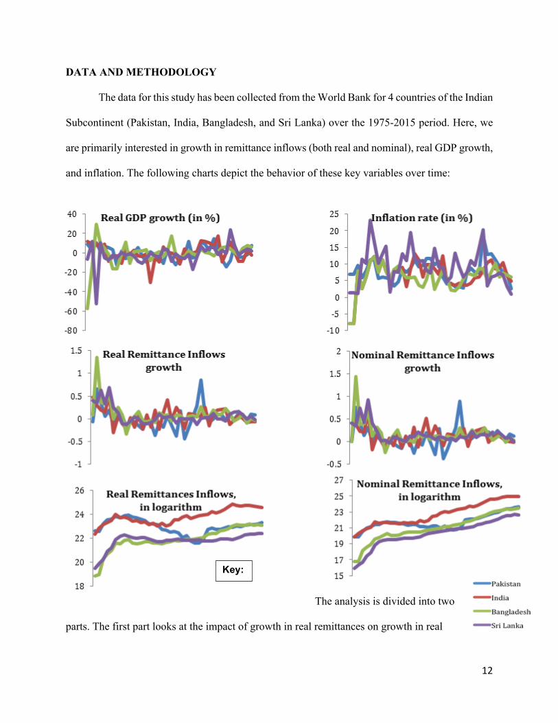
DATA AND METHODOLOGY
The data for this study has been collected from the World Bank for 4 countries of the Indian
Subcontinent (Pakistan, India, Bangladesh, and Sri Lanka) over the 1975-2015 period. Here, we
are primarily interested in growth in remittance inflows (both real and nominal), real GDP growth,
and inflation. The following charts depict the behavior of these key variables over time:
The analysis is divided into two
parts. The first part looks at the impact of growth in real remittances on growth in real
Key:
13
GDP, while the second part examines the impact of growth in nominal remittances on inflation.
Four models are estimated for each, all using panel data from 1975 through 2015. The first
model does not include fixed effects, while the second model includes both time and country
fixed effects. Next, separate Wald tests are conducted to see if the time dummy variables and the
country dummy variables are needed. Then, based on the Wald test results in Model 2, we
estimate Models 3 and 4. Model 4 includes four interaction variables in order to identify the
effects on individual countries separately. Finally, we conduct the Wald test in order to see
whether it is reasonable to assume that remittance inflows affect real GDP and inflation of the
four countries differently.
In the second part for inflation, we initially thought of using one-year lags for growth in
nominal remittance inflows, because we expected the effect of remittance inflow growth on
inflation would not be realized immediately as explained by the Keynesian view of sticky prices.
Not all remittances are consumed simultaneously as they are received by the households, and even
if they were to be consumed immediately, the price levels may not change immediately. However,
based on the preliminary estimations, we found that the effect of remittance inflows was realized
within a year, and hence the lagged variables were not used for the estimations in this paper.
Furthermore, since it is essential to take into consideration other factors that may play a
role in affecting the dependent variables, we include several control variables from economic
theory: These are growth in government spending, money supply, consumption, exports and
imports of goods and services, and population in addition to the rate of depreciation in the domestic
currency. Details of these variables are provided in the following table:
14
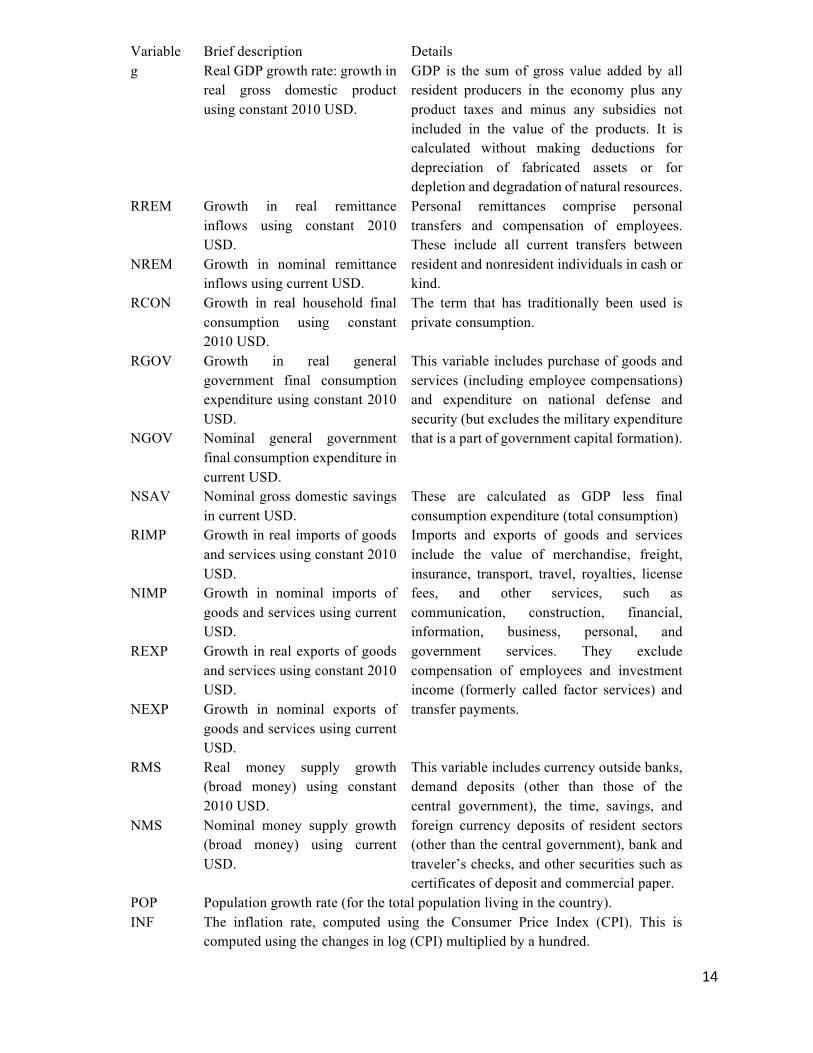
Variable Brief description Details g Real GDP growth rate: growth in
real gross domestic product using constant 2010 USD.
GDP is the sum of gross value added by all resident producers in the economy plus any product taxes and minus any subsidies not included in the value of the products. It is calculated without making deductions for depreciation of fabricated assets or for depletion and degradation of natural resources.
RREM Growth in real remittance inflows using constant 2010 USD.
Personal remittances comprise personal transfers and compensation of employees. These include all current transfers between resident and nonresident individuals in cash or kind.
NREM Growth in nominal remittance inflows using current USD.
RCON Growth in real household final consumption using constant 2010 USD.
The term that has traditionally been used is private consumption.
RGOV Growth in real general government final consumption expenditure using constant 2010 USD.
This variable includes purchase of goods and services (including employee compensations) and expenditure on national defense and security (but excludes the military expenditure that is a part of government capital formation). NGOV Nominal general government
final consumption expenditure in current USD.
NSAV Nominal gross domestic savings in current USD.
These are calculated as GDP less final consumption expenditure (total consumption)
RIMP Growth in real imports of goods and services using constant 2010 USD.
Imports and exports of goods and services include the value of merchandise, freight, insurance, transport, travel, royalties, license fees, and other services, such as communication, construction, financial, information, business, personal, and government services. They exclude compensation of employees and investment income (formerly called factor services) and transfer payments.
NIMP Growth in nominal imports of goods and services using current USD.
REXP Growth in real exports of goods and services using constant 2010 USD.
NEXP Growth in nominal exports of goods and services using current USD.
RMS Real money supply growth (broad money) using constant 2010 USD.
This variable includes currency outside banks, demand deposits (other than those of the central government), the time, savings, and foreign currency deposits of resident sectors (other than the central government), bank and traveler’s checks, and other securities such as certificates of deposit and commercial paper.
NMS Nominal money supply growth (broad money) using current USD.
POP Population growth rate (for the total population living in the country). INF The inflation rate, computed using the Consumer Price Index (CPI). This is
computed using the changes in log (CPI) multiplied by a hundred.
15
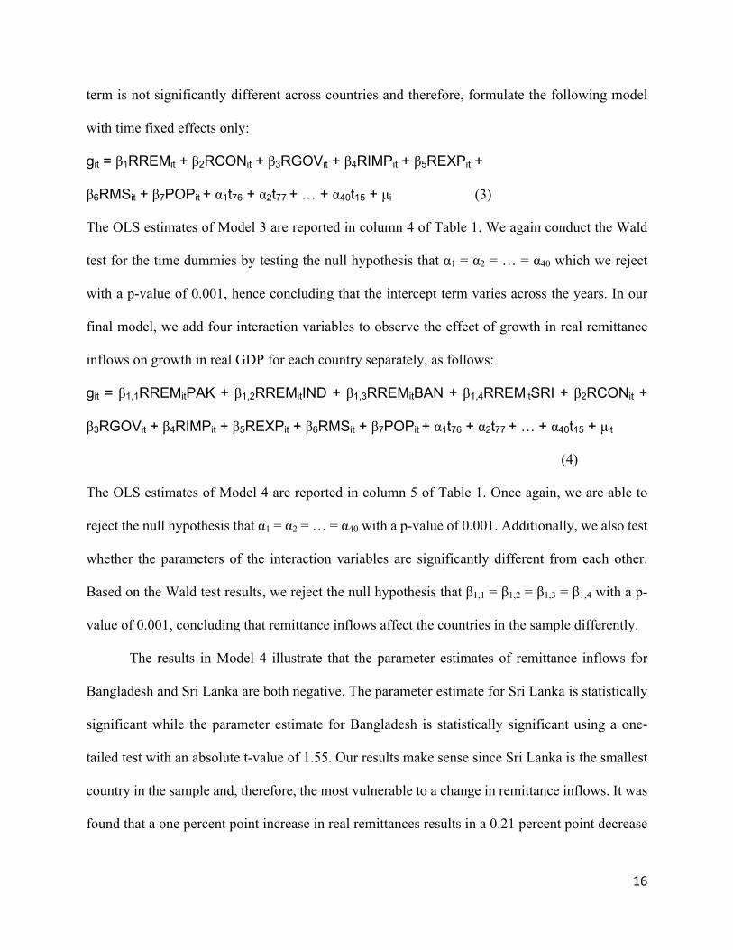
EMPIRICAL ESTIMATIONS AND RESULTS
This section is divided into two parts. The first part examines the effect of real remittance
growth on real economic growth, and the second part studies the effect of nominal remittance
growth on inflation.
EMPIRICAL ESTIMATIONS AND RESULTS FOR REAL GDP GROWTH
Model 1 for real GDP growth contains no fixed effects as follows:
git = α0 + β1RREMit + β3RCONit + β4RGOVit + β5RIMPit + β6REXPit +
β7RMSit + β8POPit + µit (1)
The OLS estimates of Model 1 are reported in column 2 of Table 1. We then include time and
country fixed effects using dummy variables in the following model:
git = β1RREMit + β2RCONit + β3RGOVit + β4RIMPit + β5REXPit + β6RMSit + β7POPit +
α1t77 + α2t78 + … + α39t15 + ϒ1PAK + ϒ2IND + ϒ3BAN + ϒ4SRI + µit (2)
The OLS estimates of Model 2 are reported in column 3 of Table 1. Next, we conduct separate
Wald tests on the fixed effect dummy variables. We reject the null hypothesis that α1 = α2 = … =
α39 with a p-value of 0.001, concluding that the intercept term significantly varies across time and
therefore, the time dummy variables are collectively considered important in the model. However,
when we repeat the test for the country dummy variables, we are unable to reject the null
hypothesis that ϒ1 = ϒ2 = ϒ3 = ϒ4 with a p-value of 0.466. Therefore, we conclude that the intercept
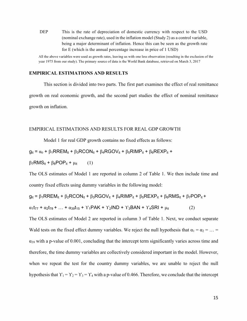
DEP This is the rate of depreciation of domestic currency with respect to the USD (nominal exchange rate), used in the inflation model (Study 2) as a control variable, being a major determinant of inflation. Hence this can be seen as the growth rate for E (which is the annual percentage increase in price of 1 USD)
All the above variables were used as growth rates, leaving us with one less observation (resulting in the exclusion of the year 1975 from our study). The primary source of data is the World Bank database, retrieved on March 3, 2017
16
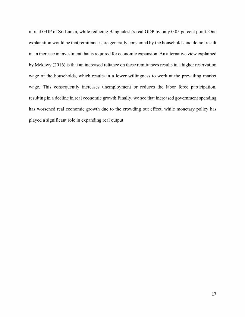
term is not significantly different across countries and therefore, formulate the following model
with time fixed effects only:
git = β1RREMit + β2RCONit + β3RGOVit + β4RIMPit + β5REXPit +
β6RMSit + β7POPit + α1t76 + α2t77 + … + α40t15 + µi (3)
The OLS estimates of Model 3 are reported in column 4 of Table 1. We again conduct the Wald
test for the time dummies by testing the null hypothesis that α1 = α2 = … = α40 which we reject
with a p-value of 0.001, hence concluding that the intercept term varies across the years. In our
final model, we add four interaction variables to observe the effect of growth in real remittance
inflows on growth in real GDP for each country separately, as follows:
git = β1,1RREMitPAK + β1,2RREMitIND + β1,3RREMitBAN + β1,4RREMitSRI + β2RCONit +
β3RGOVit + β4RIMPit + β5REXPit + β6RMSit + β7POPit + α1t76 + α2t77 + … + α40t15 + µit
(4)
The OLS estimates of Model 4 are reported in column 5 of Table 1. Once again, we are able to
reject the null hypothesis that α1 = α2 = … = α40 with a p-value of 0.001. Additionally, we also test
whether the parameters of the interaction variables are significantly different from each other.
Based on the Wald test results, we reject the null hypothesis that β1,1 = β1,2 = β1,3 = β1,4 with a p-
value of 0.001, concluding that remittance inflows affect the countries in the sample differently.
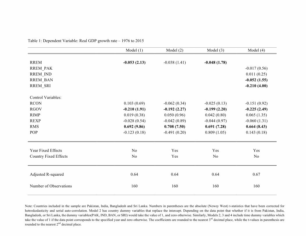
The results in Model 4 illustrate that the parameter estimates of remittance inflows for
Bangladesh and Sri Lanka are both negative. The parameter estimate for Sri Lanka is statistically
significant while the parameter estimate for Bangladesh is statistically significant using a one-
tailed test with an absolute t-value of 1.55. Our results make sense since Sri Lanka is the smallest
country in the sample and, therefore, the most vulnerable to a change in remittance inflows. It was
found that a one percent point increase in real remittances results in a 0.21 percent point decrease
17
in real GDP of Sri Lanka, while reducing Bangladesh’s real GDP by only 0.05 percent point. One
explanation would be that remittances are generally consumed by the households and do not result
in an increase in investment that is required for economic expansion. An alternative view explained
by Mekawy (2016) is that an increased reliance on these remittances results in a higher reservation
wage of the households, which results in a lower willingness to work at the prevailing market
wage. This consequently increases unemployment or reduces the labor force participation,
resulting in a decline in real economic growth.Finally, we see that increased government spending
has worsened real economic growth due to the crowding out effect, while monetary policy has
played a significant role in expanding real output
18
Table 1: Dependent Variable: Real GDP growth rate – 1976 to 2015
Model (1) Model (2) Model (3) Model (4)
RREM -0.053 (2.13) -0.038 (1.41) -0.048 (1.78) RREM_PAK -0.017 (0.56) RREM_IND 0.011 (0.25) RREM_BAN -0.052 (1.55) RREM_SRI -0.210 (4.00)
Control Variables: RCON 0.103 (0.69) -0.062 (0.34) -0.025 (0.13) -0.151 (0.92) RGOV -0.210 (1.91) -0.192 (2.27) -0.199 (2.20) -0.225 (2.49) RIMP 0.019 (0.38) 0.050 (0.96) 0.042 (0.80) 0.065 (1.35) REXP -0.028 (0.54) -0.042 (0.89) -0.044 (0.97) -0.060 (1.31) RMS 0.692 (9.86) 0.708 (7.50) 0.691 (7.28) 0.664 (8.43) POP -0.123 (0.18) -0.491 (0.20) 0.809 (1.05) 0.143 (0.18)
Year Fixed Effects No Yes Yes Yes Country Fixed Effects No Yes No No
Adjusted R-squared 0.64 0.64 0.64 0.67
Number of Observations 160 160 160 160
Note: Countries included in the sample are Pakistan, India, Bangladesh and Sri Lanka. Numbers in parentheses are the absolute (Newey West) t-statistics that have been corrected for hetroskedasticity and serial auto-correlation. Model 2 has country dummy variables that replace the intercept. Depending on the data point that whether if it is from Pakistan, India, Bangladesh, or Sri Lanka, the dummy variables(PAK, IND, BAN, or SRI) would take the value of 1, and zero otherwise. Similarly, Models 2, 3 and 4 include time dummy variables which take the value of 1 if the data point corresponds to the specified year and zero otherwise. The coefficients are rounded to the nearest 3rd decimal place, while the t-values in parenthesis are rounded to the nearest 2nd decimal place.
19
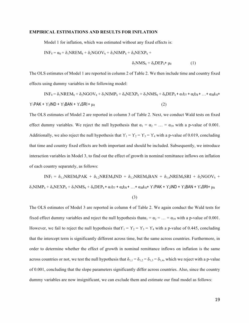
EMPIRICAL ESTIMATIONS AND RESULTS FOR INFLATION
Model 1 for inflation, which was estimated without any fixed effects is:
INFit = α0 + δ1NREMit + δ2NGOVit + δ3NIMPit + δ4NEXPit +
δ5NMSit + δ6DEPit+ µit (1)
The OLS estimates of Model 1 are reported in column 2 of Table 2. We then include time and country fixed
effects using dummy variables in the following model:
INFit = δ1NREMit + δ2NGOVit + δ3NIMPit + δ4NEXPit + δ5NMSit + δ6DEPit + α1t77 + α2t78 + …+ α39t15+
ϒ1PAK + ϒ2IND + ϒ3BAN + ϒ4SRI + µit (2)
The OLS estimates of Model 2 are reported in column 3 of Table 2. Next, we conduct Wald tests on fixed
effect dummy variables. We reject the null hypothesis that α1 = α2 = … = α39 with a p-value of 0.001.
Additionally, we also reject the null hypothesis that ϒ1 = ϒ2 = ϒ3 = ϒ4 with a p-value of 0.019, concluding
that time and country fixed effects are both important and should be included. Subsequently, we introduce
interaction variables in Model 3, to find out the effect of growth in nominal remittance inflows on inflation
of each country separately, as follows:
INFt = δ1,1NREMitPAK + δ1,2NREMitIND + δ1,3NREMitBAN + δ1,4NREMitSRI + δ2NGOVit +
δ3NIMPit + δ4NEXPit + δ5NMSit + δ6DEPit + α1t77 + α2t78 + …+ α39t15+ ϒ1PAK + ϒ2IND + ϒ3BAN + ϒ4SRI+ µit
(3)
The OLS estimates of Model 3 are reported in column 4 of Table 2. We again conduct the Wald tests for
fixed effect dummy variables and reject the null hypothesis thatα1 = α2 = … = α39 with a p-value of 0.001.
However, we fail to reject the null hypothesis thatϒ1 = ϒ2 = ϒ3 = ϒ4 with a p-value of 0.445, concluding
that the intercept term is significantly different across time, but the same across countries. Furthermore, in
order to determine whether the effect of growth in nominal remittance inflows on inflation is the same
across countries or not, we test the null hypothesis that δ1,1 = δ1,2 = δ1,3 = δ1,4, which we reject with a p-value
of 0.001, concluding that the slope parameters significantly differ across countries. Also, since the country
dummy variables are now insignificant, we can exclude them and estimate our final model as follows:
20
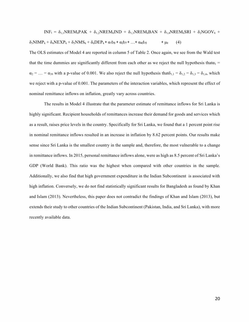
INFt = δ1,1NREMitPAK + δ1,2NREMitIND + δ1,3NREMitBAN + δ1,4NREMitSRI + δ2NGOVit +
δ3NIMPit + δ4NEXPit + δ5NMSit + δ6DEPit + α1t76 + α2t77 + …+ α40t15 + µit (4)
The OLS estimates of Model 4 are reported in column 5 of Table 2. Once again, we see from the Wald test
that the time dummies are significantly different from each other as we reject the null hypothesis thatα1 =
α2 = … = α39 with a p-value of 0.001. We also reject the null hypothesis thatδ1,1 = δ1,2 = δ1,3 = δ1,4, which
we reject with a p-value of 0.001. The parameters of the interaction variables, which represent the effect of
nominal remittance inflows on inflation, greatly vary across countries.
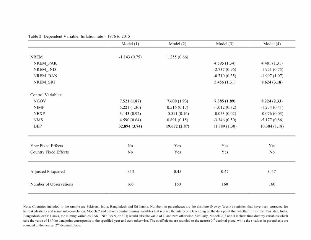
The results in Model 4 illustrate that the parameter estimate of remittance inflows for Sri Lanka is
highly significant. Recipient households of remittances increase their demand for goods and services which
as a result, raises price levels in the country. Specifically for Sri Lanka, we found that a 1 percent point rise
in nominal remittance inflows resulted in an increase in inflation by 8.62 percent points. Our results make
sense since Sri Lanka is the smallest country in the sample and, therefore, the most vulnerable to a change
in remittance inflows. In 2015, personal remittance inflows alone, were as high as 8.5 percent of Sri Lanka’s
GDP (World Bank). This ratio was the highest when compared with other countries in the sample.
Additionally, we also find that high government expenditure in the Indian Subcontinent is associated with
high inflation. Conversely, we do not find statistically significant results for Bangladesh as found by Khan
and Islam (2013). Nevertheless, this paper does not contradict the findings of Khan and Islam (2013), but
extends their study to other countries of the Indian Subcontinent (Pakistan, India, and Sri Lanka), with more
recently available data.
1
Table 2: Dependent Variable: Inflation rate – 1976 to 2015
Model (1) Model (2) Model (3) Model (4)
NREM -1.143 (0.75) 1.255 (0.66) NREM_PAK 4.595 (1.34) 4.481 (1.31) NREM_IND -2.737 (0.96) -1.921 (0.75) NREM_BAN -0.710 (0.35) -1.997 (1.07) NREM_SRI 5.456 (1.31) 8.624 (3.18)
Control Variables: NGOV 7.521 (1.87) 7.600 (1.93) 7.385 (1.89) 8.224 (2.33) NIMP 5.221 (1.30) 0.516 (0.17) -1.012 (0.32) -1.274 (0.41) NEXP 3.143 (0.92) -0.511 (0.16) -0.053 (0.02) -0.076 (0.03) NMS 4.590 (0.64) 0.891 (0.15) -3.346 (0.50) -5.177 (0.86) DEP 32.894 (3.74) 19.672 (2.87) 11.889 (1.30) 10.384 (1.18)
Year Fixed Effects No Yes Yes Yes Country Fixed Effects No Yes Yes No
Adjusted R-squared 0.13 0.45 0.47 0.47
Number of Observations 160 160 160 160
Note: Countries included in the sample are Pakistan, India, Bangladesh and Sri Lanka. Numbers in parentheses are the absolute (Newey West) t-statistics that have been corrected for hetroskedasticity and serial auto-correlation. Models 2 and 3 have country dummy variables that replace the intercept. Depending on the data point that whether if it is from Pakistan, India, Bangladesh, or Sri Lanka, the dummy variables(PAK, IND, BAN, or SRI) would take the value of 1, and zero otherwise. Similarly, Models 2, 3 and 4 include time dummy variables which take the value of 1 if the data point corresponds to the specified year and zero otherwise. The coefficients are rounded to the nearest 3rd decimal place, while the t-values in parenthesis are rounded to the nearest 2nd decimal place.

22
CONCLUSION AND POLICY RECOMMENDATIONS
The findings of this paper show that remittance inflows have adversely affected real
economic growth of Bangladesh and Sri Lanka during the period 1976-2015. Additionally, over
the same period, faster growth in remittance inflows resulted in higher inflation in Sri Lanka. Both
these factors tell us that remittance inflows would serve as a very poor macroeconomic tool for
development.
As households in Bangladesh and Sri Lanka get more and more remittances, their
reservation wage rises, which means that they would no longer be willing to work at a wage that
they would otherwise have happily accepted. Hence, although these remittances may improve their
living standards, they may reduce the likelihood that the receivers would participate in the labor
force, which would, as a result, hinder economic growth.
Also, what we deduce from the findings of this paper is that macroeconomic policies for
developing countries must be carefully devised, considering the potential impact that remittance
inflows would have on inflation. In particular, they must consider that remittance inflows would
cause inflation as we see in the case of Sri Lanka. It is, therefore, important to understand that
depending on a continued source of funds from other countries may not be an optimal solution
for the developing world. Sri Lanka in particular, should, therefore, reduce their reliance on
remittance inflows and attempt to achieve real economic growth through other competitive
means such as trade, commerce, and industry. In general, developing countries must create
opportunities for their workforce domestically, by providing the necessary infrastructure, law
and order to enable the hardworking population to prosper without having to migrate to a foreign
land.
23
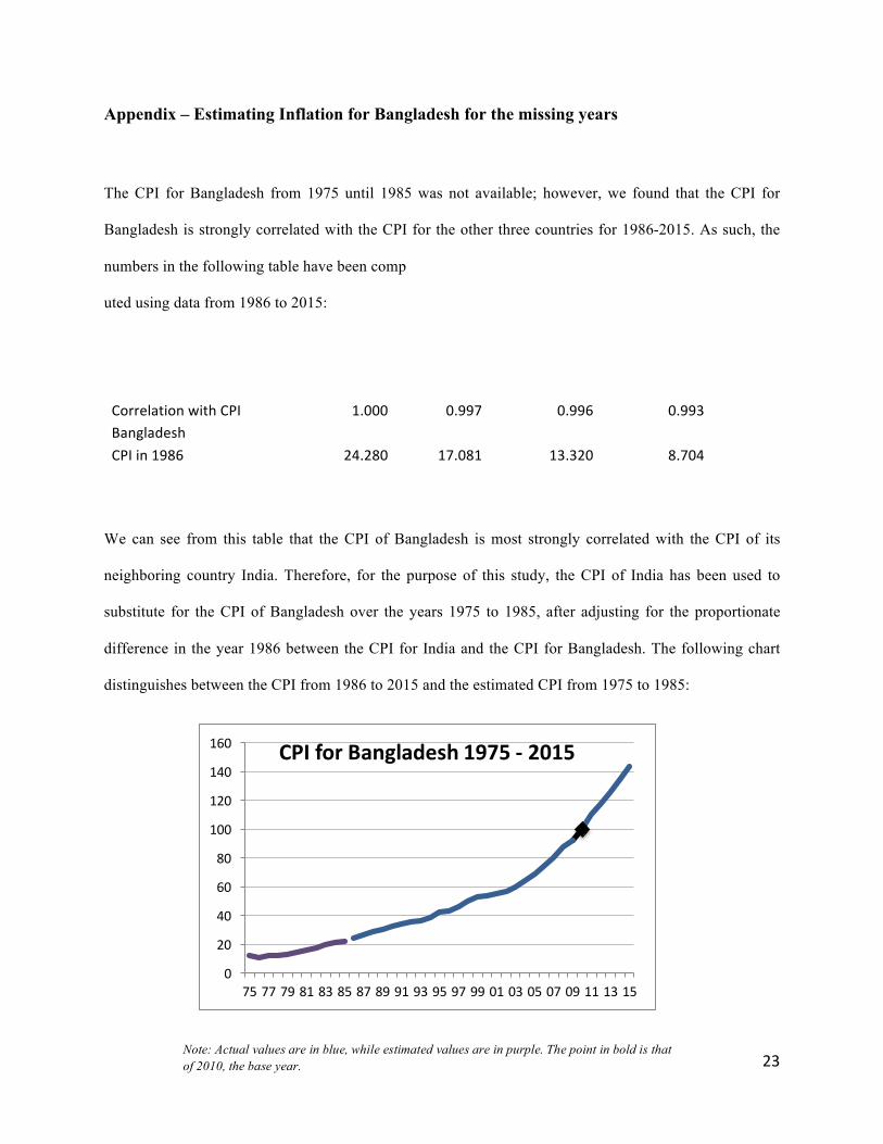
Appendix – Estimating Inflation for Bangladesh for the missing years
The CPI for Bangladesh from 1975 until 1985 was not available; however, we found that the CPI for
Bangladesh is strongly correlated with the CPI for the other three countries for 1986-2015. As such, the
numbers in the following table have been comp
uted using data from 1986 to 2015:
We can see from this table that the CPI of Bangladesh is most strongly correlated with the CPI of its
neighboring country India. Therefore, for the purpose of this study, the CPI of India has been used to
substitute for the CPI of Bangladesh over the years 1975 to 1985, after adjusting for the proportionate
difference in the year 1986 between the CPI for India and the CPI for Bangladesh. The following chart
distinguishes between the CPI from 1986 to 2015 and the estimated CPI from 1975 to 1985:
CPIBangladesh CPIIndia CPIPakistan CPISriLankaCorrelationwithCPIBangladesh
1.000 0.997 0.996 0.993
CPIin1986 24.280 17.081 13.320 8.704
0
20
40
60
80
100
120
140
160
75 77 79 81 83 85 87 89 91 93 95 97 99 01 03 05 07 09 11 13 15
CPIforBangladesh1975- 2015
Note: Actual values are in blue, while estimated values are in purple. The point in bold is that of 2010, the base year.
24
References
Adams, R. H., & Page, J. (2005). Do international migration and remittances reduce poverty in developing
countries?World Development, 33(10), 1645-1669.
Akter, S. (2016). Remittance inflows and its contribution to the economic growth of Bangladesh, research
report, Niigata University. Retrieved fromhttp://dspace.lib.niigata-
u.ac.jp/dspace/bitstream/10191/41800/1/62_215-245.pdf
Al-Kaabi, F. (2016).The nexus between remittance outflows and GCC growth and inflation.Journal of
International Business and Economics, 4(1), 76-84.
Barajas, A., Chami, R., Fullenkamp, C., Gapen, M., &Montiel, P. J. (2009). Do workers' remittances
promote economic growth? IMF working papers.Retrieved from
https://www.imf.org/external/pubs/cat/longres.aspx?sk=23108.0
Durand, J., Kandel, W., Parrado, E. A., & Massey, D. S. (1996).International migration and development
in Mexican communities.Demography, 33(2), 249-264.
Hung, T. N., & Minh, N. (2014). Do workers’ remittances induce inflation? The case of Vietnam, 1996-
2012.Review of Business and Economics Studies, (1), 39-48.
Khan, Z. S., & Islam, S. (2013). The effects of remittances on inflation: Evidence from Bangladesh. Journal
of Economics and Business Research, 19(2), 198-208.
Mekawy, A. A. (2016). Remittance inflows and labor markets: Evidence from North Africa, research report,
American University of Sharjah.
Narayan, P. K., Narayan, S., & Mishra, S. (2011). Do remittances induce inflation? Fresh evidence from
developing countries.Southern Economic Journal, 77(4), 914-933.
Ulyses Balderas, J., &Nath, H. K. (2008). Inflation and relative price variability in Mexico: The role of
remittances. Applied Economics Letters, 15(3), 181-185.
Zarate-Hoyos, G. A. (2004). Consumption and remittances in migrant households: Toward a productive
use of remittances. Contemporary Economic Policy, 22(4), 555-565.
25
USING PROFESSIONAL PREDICTIONS OF OUTPUT AND INFLATION TO FORECAST THE US 10-YEAR TREASURY RATE
Karam Jarad
School of Business Administration American University of Sharjah
Email: [email protected]
ABSTRACT
Economic agents and policy-makers constantly seek for accurate forecasts of macroeconomic
variables, with the interest rate receiving the widest attention. In this paper, we focus on
forecasting the US 10-year Treasury bond rate (TBR) by using professional forecasts of output
growth and inflation from the Survey of Professional Forecasters (SPF). Specifically, we
formulate a vector autoregressive (VAR) model with three variables; the TBR, the SPF forecasts
of output growth, and the SPF forecasts of inflation. Using recursive estimation, with the data
starting from 1981, we generate the one-, two-, three-, four-quarter-ahead forecasts of the TBR
for 1992-2016. Our results show that both the SPF and VAR forecasts are biased. However, we
find that the two-, 3, and four-quarter-ahead VAR forecasts contain distinct information from
those of the random walk forecasts, and combining the VAR and random walk forecasts improve
accuracy. This indicates that researchers can utilize the SPF forecasts of output growth and
inflation in order to produce more accurate forecasts of the TBR.
26
INTRODUCTION
Economic agents and policymakers constantly seek for accurate forecasts of
macroeconomic and financial variables, with the interest rate receiving the widest attention. This
is due to the fact that agents need accurate forecasts of interest rates in order to make more
informed saving and investments decisions. Similarly, policy makers need accurate forecasts in
order to make more informed macroeconomic policy decisions.
In this paper, we focus on forecasting the US 10-year Treasury bond rate (TBR), which is
used as a benchmark in pricing mortgages and many other types of consumer loans. The TBR is
also among the leading indicators for US economic activity. Due to its importance, there are
various surveys aiming to collect the forecasts of the TBR. One of these is the Survey of
Professional Forecasts (SPF), conducted quarterly by the Federal Reserve Bank of Philadelphia.
The SPF collects the professional forecasts of the TBR in addition to the forecasts of output
growth, inflation, and other major indicators.
The purpose of this paper is to use a vector autoregressive (VAR) model in order to forecast
the TBR. This VAR model includes three variables: the TBR, the SPF forecasts of output growth,
and the SPF forecasts of inflation. We use recursive information with the data starting from 1981
to generate the one-, two-, three-, and four-quarter-ahead forecasts for 1992-2016.
We then compare the VAR forecasts to the SPF and random walk forecasts of the TBR.
Our results show that both the SPF forecasts and VAR forecasts of TBR are biased, and, consistent
with the efficient market hypothesis, fail to beat random walk forecasts. However, we find that the
two-, three-, and four-quarter-ahead VAR forecasts contain distinct information from that of the
random walk forecasts, and combining the VAR and random walk forecasts improve accuracy.
27
Based on our findings, we recommend researchers utilize the SPF forecasts of output growth and
inflation in order to produce accurate forecasts of the TBR.
This paper is organized as follows: Section 2 includes the literature review. Section 3
describes the data, the SPF, VAR, and random walk forecasts of the TBR. Section 4 presents the
forecast evaluation results. Finally, Section 5 summarizes our findings and concludes the paper.
LITERATURE REVIEW
In this section, we first present the efficient market hypothesis, which simply states that the
best forecast of the long-term interest rate is today’s rate (Reichenstein, 2006, p.116). We then go
on to review the empirical findings of the existing studies in the literature.
EFFICIENT MARKET HYPOTHESIS
The efficient market hypothesis states that it is impossible to beat a random walk forecast.
This is because the random walk forecast includes all the relevant information that is required for
forecasting future rates. To demonstrate, let !" represent the one-period forward rate at time t and
#$," denote the pure discount (or spot) rate at time t on an n-period bond. According to the pure
expectations hypothesis, the forward rate at time t is equal to the expected one-period discount rate
at time t (denoted by &"), Therefore, !"= &" implies that:
(1 + #$,")$ = (1 + &")(1 + &"+,)(1 + &"+-)… (1 + &"+$/,))
In other words, the pure expectations theory argues that that today’s n-period discount rate
is the average of today’s one-period discount rate and one-period discount rates expected to prevail
over the next n-1 periods (Reichenstein, 2006). Raising to the power of ,$ and subtracting both
sides by 1 gives us:
#$,"=(1 + &")(1 + &"+,)(1 + &"+-)… 1 + &"+$/,) )01 - 1
28
Substituting !" back instead of &" for clarification purposes and taking the linearized version of this
equation shows the following (Schiller, 1979):
#$,"+, − #$,"= ,$ (( !"+$ "+, - !" ") + ( !"+, "+, - !"+, ") + … + ( !"+$/, "+, − !"+$/, "))
Here, !"+, " represents the one-period forward rate found at time t for period t+1. Taking the
expectation of both sides, we have:
3"[#$,"+,] - #$," = ,$ ( !"+$ " − !" ") (1)
The right side of the equation goes to zero as n approaches a large number, thus we will end up
with the following simple equation:
3"[#$,"+,]≈#$,"
which states that the optimal forecast of the long-term interest rate is today’s rate. If we relax the
the time-invariant term-premium assumption and include the expected change in the term premium
over time in equation (1) and substitute &"for !", we end up with:
3"[#$,"+,] - #$," = ,$ (&"+$ − &") + 3"[Ω"+,$ ] - Ω"$
which shows that if the expected near-term change in the term premium (3"[Ω"+,$ ] - Ω"$) at time t
is minimal then, again, the long-term interest rate exhibits the characteristics of a random walk.
Given the above equation, we cannot make any theoretical conclusions about the behavior of the
short-term interest rates. That is, the short-term interest rates (&") may or may not exhibit random
walk behavior and, as Pesando (1979) argues, it is basically an empirical question (Baghestani et
al., p. 113).
LITERATURE FINDINGS
We start off by examining Friedman’s (1980) seminal paper, “Survey evidence on the
‘rationality’ of interest rate expectations” which set a lot of groundwork for economists to study
the issue of the accuracy and usefulness of professional forecasts. Friedman studies the forecasts
29
that are collected through a survey taken by The Goldsmith Nagan Bond and Money Market Letter.
The Goldsmith Nagan letter has been conducting these surveys since 1969 by asking around 50
market professionals to provide their one- and two-quarter-ahead expectations of interest rates.
The results are then published as the consensus (mean) of the individual responses. The survey
includes 11 different types of interest rates, but Friedman’s study focuses on 6 of them: 1) federal
funds, 2) three-month US Treasury bills, 3) six-month Eurodollar certificates of deposit, 4) twelve-
month US Treasury bills, 5) new issues of high-grade long-term utility bonds, and 6) seasoned
issues of high-grade long-term municipal bonds. Friedman’s results indicate that professionals
made biased predictions and did not efficiently use the information contained in past interest rate
changes. More relevant to our paper is Friedman’s finding on the forecasts of the long-term interest
rate. His results show that professionals fail to “exploit efficiently the information contained in
common macroeconomic and macro-policy variables other than the money stock” (p. 453).
Friedman’s (1980) study has motivated researchers to further study different types of survey data
and see whether or not these forecasts are also biased and fail to account for important information.
In what follows, we look at the findings of some of these studies.
Brooks and Gray (2004) examine the accuracy of interest rate forecasts published by the
Wall Street Journal (WSJ). The WSJ survey has been conducting a survey since 1982 by asking
around 64 experts to provide their forecasts of the short-term and long-term interest rates around
June and December of each year. Brooks and Gray find that the WSJ consensus (mean) forecasts
predict the directional change of the TBR correctly only 35% of the time. Furthermore, the forecast
errors of the naïve forecasts are lower than those of the WSJ consensus forecasts, indicating that
the consensus forecasts are less accurate than the random walk.
30
Reichenstein (2006) shows that Brooks and Gray’s results are consistent with the efficient
market hypothesis and other empirical work. He goes on to argue that the naive model provides
not only more accurate forecasts but also pass several tests which indicate that the naive forecast
is rational.
Mitchell and Pearce (2007) also look at the survey forecasts published by the Wall Street
Journal. They show that most experts produce unbiased forecasts but none of them beat the random
walk when it comes to directional change. Furthermore, they also find that the majority of survey
forecasts of short-term interest rates are as accurate as the naïve forecasts. On the other hand, the
survey forecasts of long-term interest rates are less accurate than the naïve forecasts.
Several other studies examine the accuracy of Blue Chip consensus forecasts of interest
rates. The Blue Chip surveys around 50 professional forecasters around the beginning of each
month. The survey participants are asked to provide their forecasts of interest rates for the current
quarter, one-, two-, three-, and four-quarter-ahead. Then, the survey uses the individual forecasts
to calculate and report the consensus (median) response in theBlue Chip Financial Forecasts
(BCFF). Baghestani (2009) finds that the Blue Chip consensus forecasts of the TBR and Moody’s
Aaa corporate bond rate are biased and inferior to the random walk forecasts. In addition, these
forecasts fail to accurately predict directional change. Therefore, we can see that the results
obtained by Brooks and Gray (2004), Reichenstein (2006), Mitchell and Pearce (2007), and
Baghestani (2009) all converge towards agreeing with the efficient market hypothesis, since they
all show that professional forecasts are inferior to random walk forecasts.
Next, Baghestani et al. (2015) look at the accuracy of Blue Chip forecasts of short and
long-term interest rates in addition to forecasts of the country risk premium for several countries
for 1999-2008. They show that the long-term interest rate forecasts do not beat the random walk,

31
just as the efficient market hypothesis would suggest. On the other hand, their findings on the
accuracy of short-term forecasts are mixed. Furthermore, Baghestani et al. (2015, p. 1) show that
“Blue Chip is more (less) accurate in predicting country risk premiums associated with short-term
(long-term) interest rates”.
However, in another study, Baghestani’s (2010) findings go against the efficient market
hypothesis. More specifically, he formulates an augmented-autoregressive (A-A) model of the
TBR that uses the predictive information in expected inflation and past information in the TBR.
He shows that the A-A forecasts outperform the random walk forecasts. Perhaps, this may be
because expectations may not be rational as assumed by the efficient market hypothesis.
THE SPF, VAR AND RANDOM WALK FORECASTS OF TBR
In the middle of every quarter, the Federal Reserve Bank of Philadelphia conducts a survey
of around 50 private professional forecasters to gather the forecasts of the TBR in addition to the
forecasts of outgrowth and inflation, among others. More specifically, each forecaster is asked to
provide their forecast for the current-quarter, one-, two-, three-, four-quarter-ahead. The survey
uses the individual forecasts to calculate and report the consensus (median) forecasts. The SPF
forecasts of TBR are available from 1992 to 2016. For example, in the middle of February 1992,
the forecasters were asked to provide their forecasts for 1992Q1, 1992Q2, 1992Q3, 1992Q4, and
1993Q1. Also, in the middle of November 2015, the forecasters were asked to provide their
forecasts for 2015Q4, 2016Q1, 2016Q2, 2016Q3, and 2016Q4. This means that the current-quarter
forecasts start from 1992Q1 and run through 2015Q4, the one-quarter-ahead forecast starts from
1992Q2 and run through 2016Q1, the two-quarter forecasts start from 1992Q3 and run through
2016Q2, the three-quarter forecasts start from 1992Q4 through 2016Q3, and the four-quarter
forecast starts from 1993Q1 through 2016Q4.
32
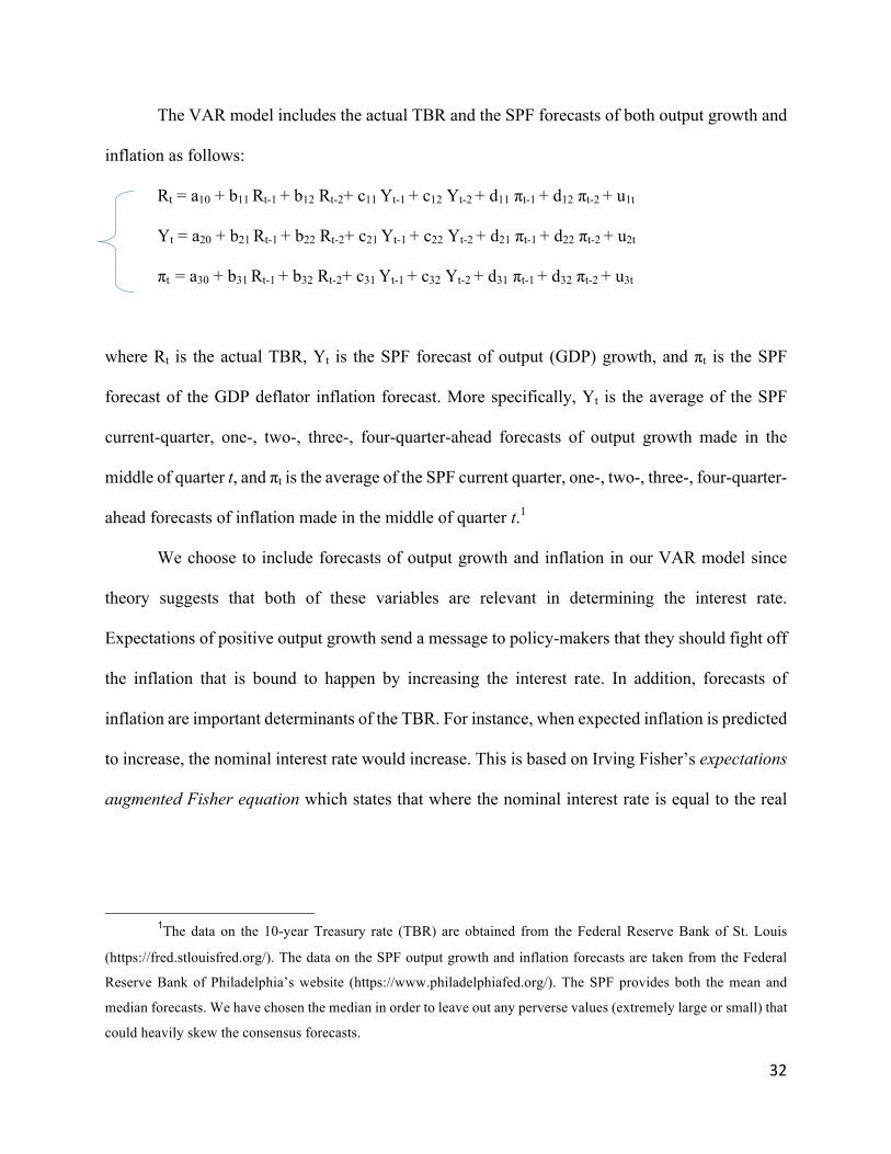
The VAR model includes the actual TBR and the SPF forecasts of both output growth and
inflation as follows:
Rt = a10 + b11 Rt-1 + b12 Rt-2+ c11 Yt-1 + c12 Yt-2 + d11 πt-1 + d12 πt-2 + u1t
Yt = a20 + b21 Rt-1 + b22 Rt-2+ c21 Yt-1 + c22 Yt-2 + d21 πt-1 + d22 πt-2 + u2t
πt = a30 + b31 Rt-1 + b32 Rt-2+ c31 Yt-1 + c32 Yt-2 + d31 πt-1 + d32 πt-2 + u3t
where Rt is the actual TBR, Yt is the SPF forecast of output (GDP) growth, and πt is the SPF
forecast of the GDP deflator inflation forecast. More specifically, Yt is the average of the SPF
current-quarter, one-, two-, three-, four-quarter-ahead forecasts of output growth made in the
middle of quarter t, and πt is the average of the SPF current quarter, one-, two-, three-, four-quarter-
ahead forecasts of inflation made in the middle of quarter t.1
We choose to include forecasts of output growth and inflation in our VAR model since
theory suggests that both of these variables are relevant in determining the interest rate.
Expectations of positive output growth send a message to policy-makers that they should fight off
the inflation that is bound to happen by increasing the interest rate. In addition, forecasts of
inflation are important determinants of the TBR. For instance, when expected inflation is predicted
to increase, the nominal interest rate would increase. This is based on Irving Fisher’s expectations
augmented Fisher equation which states that where the nominal interest rate is equal to the real
1The data on the 10-year Treasury rate (TBR) are obtained from the Federal Reserve Bank of St. Louis
(https://fred.stlouisfred.org/). The data on the SPF output growth and inflation forecasts are taken from the Federal
Reserve Bank of Philadelphia’s website (https://www.philadelphiafed.org/). The SPF provides both the mean and
median forecasts. We have chosen the median in order to leave out any perverse values (extremely large or small) that
could heavily skew the consensus forecasts.
33
interest rate plus the expected rate of inflation. Hence, it is clear that an increase in expected
inflation leads to an increase in the nominal interest rate.
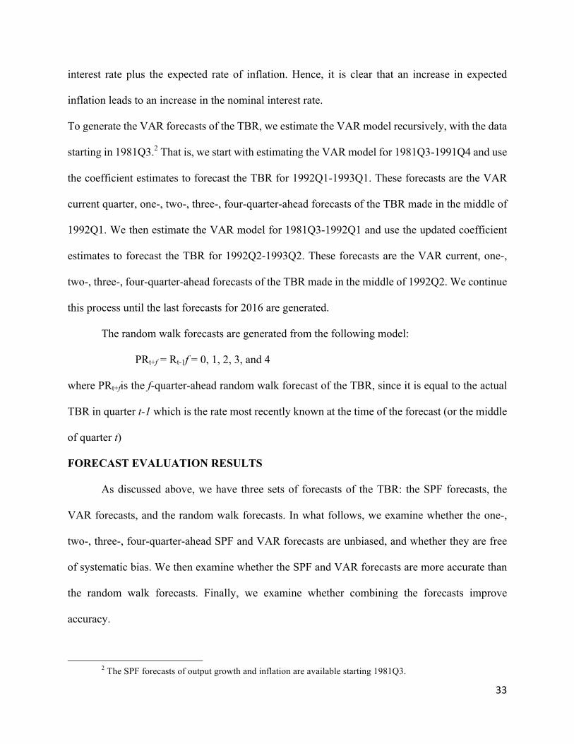
To generate the VAR forecasts of the TBR, we estimate the VAR model recursively, with the data
starting in 1981Q3.2 That is, we start with estimating the VAR model for 1981Q3-1991Q4 and use
the coefficient estimates to forecast the TBR for 1992Q1-1993Q1. These forecasts are the VAR
current quarter, one-, two-, three-, four-quarter-ahead forecasts of the TBR made in the middle of
1992Q1. We then estimate the VAR model for 1981Q3-1992Q1 and use the updated coefficient
estimates to forecast the TBR for 1992Q2-1993Q2. These forecasts are the VAR current, one-,
two-, three-, four-quarter-ahead forecasts of the TBR made in the middle of 1992Q2. We continue
this process until the last forecasts for 2016 are generated.
The random walk forecasts are generated from the following model:
PRt+f = Rt-1f = 0, 1, 2, 3, and 4
where PRt+fis the f-quarter-ahead random walk forecast of the TBR, since it is equal to the actual
TBR in quarter t-1 which is the rate most recently known at the time of the forecast (or the middle
of quarter t)
FORECAST EVALUATION RESULTS
As discussed above, we have three sets of forecasts of the TBR: the SPF forecasts, the
VAR forecasts, and the random walk forecasts. In what follows, we examine whether the one-,
two-, three-, four-quarter-ahead SPF and VAR forecasts are unbiased, and whether they are free
of systematic bias. We then examine whether the SPF and VAR forecasts are more accurate than
the random walk forecasts. Finally, we examine whether combining the forecasts improve
accuracy.
2 The SPF forecasts of output growth and inflation are available starting 1981Q3.
34
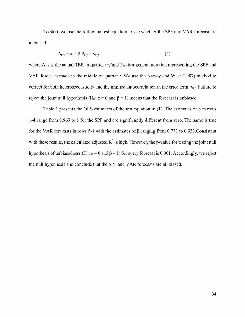
To start, we use the following test equation to see whether the SPF and VAR forecast are
unbiased:
At+f = α + β Pt+f + ut+f (1)
where At+f is the actual TBR in quarter t+f and Pt+f is a general notation representing the SPF and
VAR forecasts made in the middle of quarter t. We use the Newey and West (1987) method to
correct for both heteroscedasticity and the implied autocorrelation in the error term ut+f. Failure to
reject the joint null hypothesis (H0: α = 0 and β = 1) means that the forecast is unbiased.
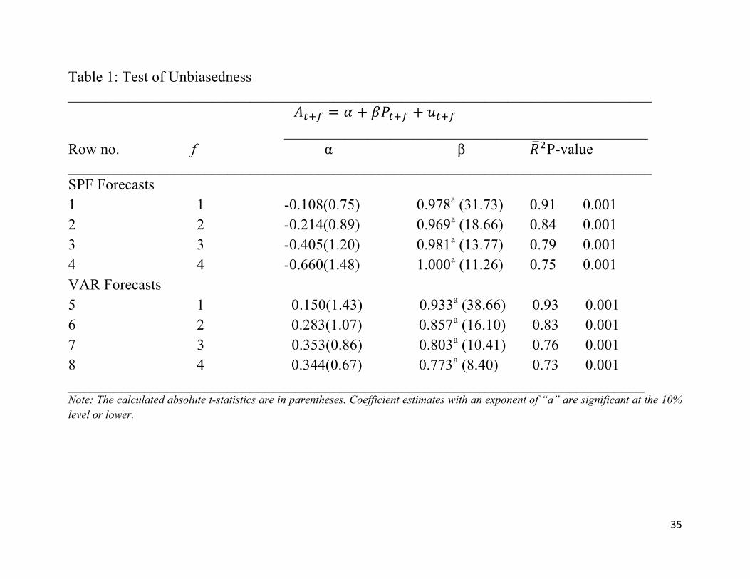
Table 1 presents the OLS estimates of the test equation in (1). The estimates of β in rows
1-4 range from 0.969 to 1 for the SPF and are significantly different from zero. The same is true
for the VAR forecasts in rows 5-8 with the estimates of β ranging from 0.773 to 0.933.Consistent
with these results, the calculated adjusted R2 is high. However, the p-value for testing the joint null
hypothesis of unbiasedness (H0: α = 0 and β = 1) for every forecast is 0.001. Accordingly, we reject
the null hypothesis and conclude that the SPF and VAR forecasts are all biased.
35
Table 1: Test of Unbiasedness _____________________________________________________________________________
!"#$ = & + ()"#$ + *"#$ ________________________________________________ Row no. f α β +,P-value _____________________________________________________________________________ SPF Forecasts 1 1 -0.108(0.75) 0.978a (31.73) 0.91 0.001 2 2 -0.214(0.89) 0.969a (18.66) 0.84 0.001 3 3 -0.405(1.20) 0.981a (13.77) 0.79 0.001 4 4 -0.660(1.48) 1.000a (11.26) 0.75 0.001 VAR Forecasts 5 1 0.150(1.43) 0.933a (38.66) 0.93 0.001 6 2 0.283(1.07) 0.857a (16.10) 0.83 0.001 7 3 0.353(0.86) 0.803a (10.41) 0.76 0.001 8 4 0.344(0.67) 0.773a (8.40) 0.73 0.001 ____________________________________________________________________________ Note: The calculated absolute t-statistics are in parentheses. Coefficient estimates with an exponent of “a” are significant at the 10% level or lower.
36
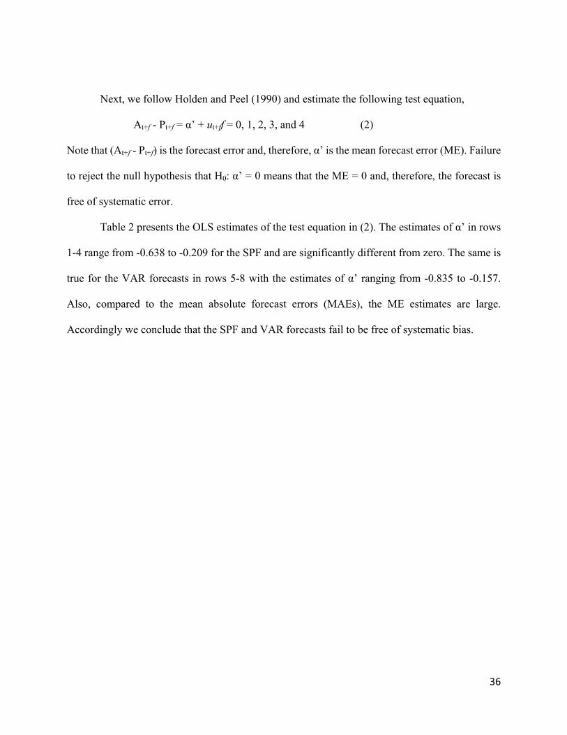
Next, we follow Holden and Peel (1990) and estimate the following test equation,
At+f - Pt+f = α’ + ut+ff = 0, 1, 2, 3, and 4 (2)
Note that (At+f - Pt+f) is the forecast error and, therefore, α’ is the mean forecast error (ME). Failure
to reject the null hypothesis that H0: α’ = 0 means that the ME = 0 and, therefore, the forecast is
free of systematic error.
Table 2 presents the OLS estimates of the test equation in (2). The estimates of α’ in rows
1-4 range from -0.638 to -0.209 for the SPF and are significantly different from zero. The same is
true for the VAR forecasts in rows 5-8 with the estimates of α’ ranging from -0.835 to -0.157.
Also, compared to the mean absolute forecast errors (MAEs), the ME estimates are large.
Accordingly we conclude that the SPF and VAR forecasts fail to be free of systematic bias.
37
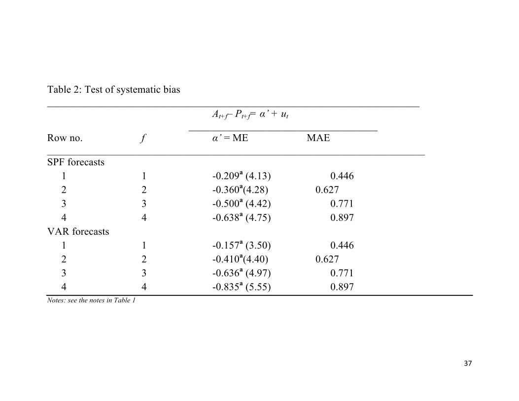
Table 2: Test of systematic bias _______________________________________________________________________ At+f– Pt+f= α’ + ut ____________________________________ Row no. f α’ = ME MAE ________________________________________________________________________ SPF forecasts 1 1 -0.209a (4.13) 0.446 2 2 -0.360a(4.28) 0.627 3 3 -0.500a (4.42) 0.771 4 4 -0.638a (4.75) 0.897 VAR forecasts 1 1 -0.157a (3.50) 0.446 2 2 -0.410a(4.40) 0.627 3 3 -0.636a (4.97) 0.771 4 4 -0.835a (5.55) 0.897 Notes: see the notes in Table 1

38
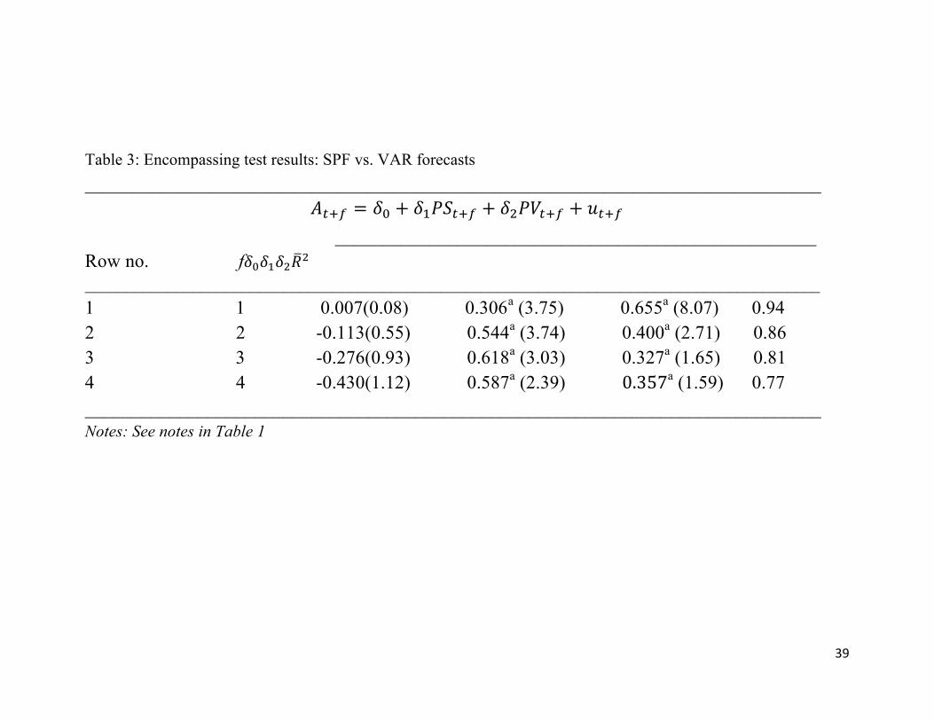
Next, we compare the SPF and VAR forecasts in terms of predictive information by
estimating the following test equation:
!"#$ = &' + &)*+"#$ + &,*-"#$ + ."#$ (3)
where*+"#$ represents the SPF forecasts while *-"#$ represents the VAR forecasts in quarter t
+ f. The possible outcomes for this encompassing test are:
1) The coefficient estimates of &) and&, are both positive and significant. This means
thatPSt+fandPVt+fcontain distinct information.
2) The coefficient estimate of &) is positive and significant but the coefficient estimate
of &, is negative or insignificant. This means that PSt+fissuperior to PVt+f.
3) The coefficient estimate of &, is positive and significant but the coefficient estimate
of &) is negative or insignificant. This means PVt+f is superior toPSt+f.
4) The coefficient estimates of &) and &, are both insignificant but the population/, ≠
0. This means that the PSt+fandPVt+f contain similar information.
Table 3 presents the OLS estimates of the test equation in (3). The estimates of &), ranging from
0.306 to 0.618, are positive and significant. Similarly, the estimates of &,, ranging from 0.327 to
0.655, are positive and significant across all four forecast horizons. This implies that the VAR
forecasts contain distinct information from the SPF forecasts.
39
Table 3: Encompassing test results: SPF vs. VAR forecasts ______________________________________________________________________________
!"#$ = &' + &)*+"#$ + &,*-"#$ + ."#$ ___________________________________________________ Row no. f&'&)&,/, _________________________________________________________________________________________ 1 1 0.007(0.08) 0.306a (3.75) 0.655a (8.07) 0.94 2 2 -0.113(0.55) 0.544a (3.74) 0.400a (2.71) 0.86 3 3 -0.276(0.93) 0.618a (3.03) 0.327a (1.65) 0.81 4 4 -0.430(1.12) 0.587a (2.39) 0.357a (1.59) 0.77 ______________________________________________________________________________ Notes: See notes in Table 1

40
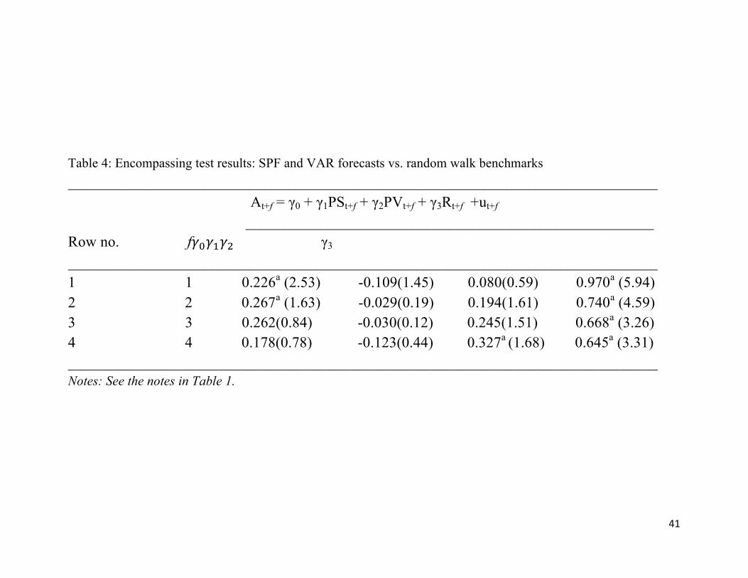
To check the robustness of these results, we also include the random walk forecasts in the
test equation as follows:
At+f = γ0 + γ1PSt+f + γ2PVt+f + γ3Rt+f +ut+f (4)
where!"#$% represents the SPF forecasts, !&#$% represents the VAR forecasts in quarter t + f, and
'#$% represents the random walk forecasts.
Table 4 presents the OLS estimates of the test equation in (4). The estimates of (), ranging
from -0.029 to -0.123, are all negative and insignificant. However, the estimates of γ2, ranging
from 0.08 to 0.327, are all positive. More importantly, the t-statistics on the estimates of γ2 in rows
2-4 are fairly large and close to the threshold for statistical significance. This implies that the two-
through the four-quarter-ahead VAR forecasts are more informative than the corresponding SPF
forecasts of the TBR and may also have distinct predictive information from the corresponding
random walk forecasts.
41
Table 4: Encompassing test results: SPF and VAR forecasts vs. random walk benchmarks ______________________________________________________________________________
At+f = γ0 + γ1PSt+f + γ2PVt+f + γ3Rt+f +ut+f ______________________________________________________ Row no. f!"!#!$ γ3
______________________________________________________________________________ 1 1 0.226a (2.53) -0.109(1.45) 0.080(0.59) 0.970a (5.94) 2 2 0.267a (1.63) -0.029(0.19) 0.194(1.61) 0.740a (4.59) 3 3 0.262(0.84) -0.030(0.12) 0.245(1.51) 0.668a (3.26) 4 4 0.178(0.78) -0.123(0.44) 0.327a (1.68) 0.645a (3.31) ______________________________________________________________________________ Notes: See the notes in Table 1.
42
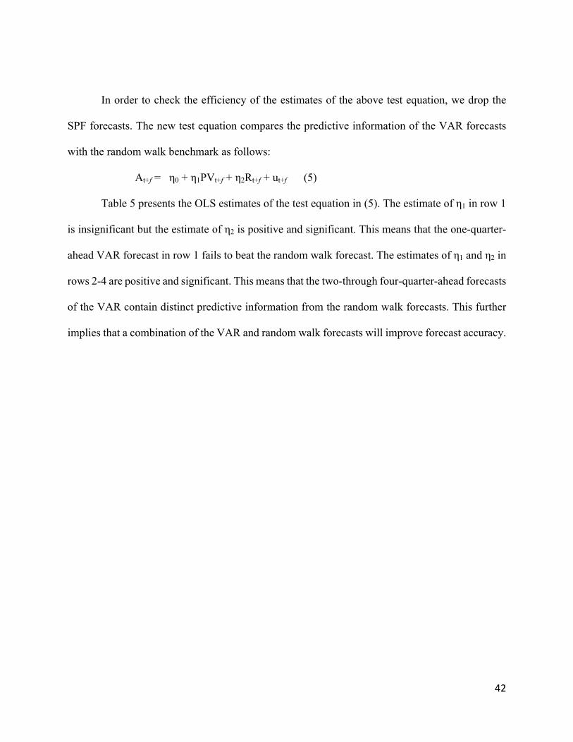
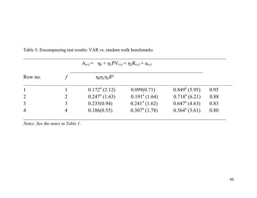
In order to check the efficiency of the estimates of the above test equation, we drop the
SPF forecasts. The new test equation compares the predictive information of the VAR forecasts
with the random walk benchmark as follows:
At+f = η0 + η1PVt+f + η2Rt+f + ut+f (5)
Table 5 presents the OLS estimates of the test equation in (5). The estimate of η1 in row 1
is insignificant but the estimate of η2 is positive and significant. This means that the one-quarter-
ahead VAR forecast in row 1 fails to beat the random walk forecast. The estimates of η1 and η2 in
rows 2-4 are positive and significant. This means that the two-through four-quarter-ahead forecasts
of the VAR contain distinct predictive information from the random walk forecasts. This further
implies that a combination of the VAR and random walk forecasts will improve forecast accuracy.
43
Table 5: Encompassing test results: VAR vs. random walk benchmarks ______________________________________________________________________________
At+f = η0 + η1PVt+f + η2Rt+f + ut+f ___________________________________________________
Row no. f η0η1η2!" ____________________________________________________________________________________________ 1 1 0.172a (2.12) 0.099(0.71) 0.849a (5.95) 0.95 2 2 0.247a (1.63) 0.191a (1.64) 0.718a (6.21) 0.88 3 3 0.235(0.94) 0.241a (1.62) 0.647a (4.63) 0.83 4 4 0.186(0.55) 0.307a (1.78) 0.564a (3.61) 0.80 ______________________________________________________________________________ Notes: See the notes in Table 1.

44
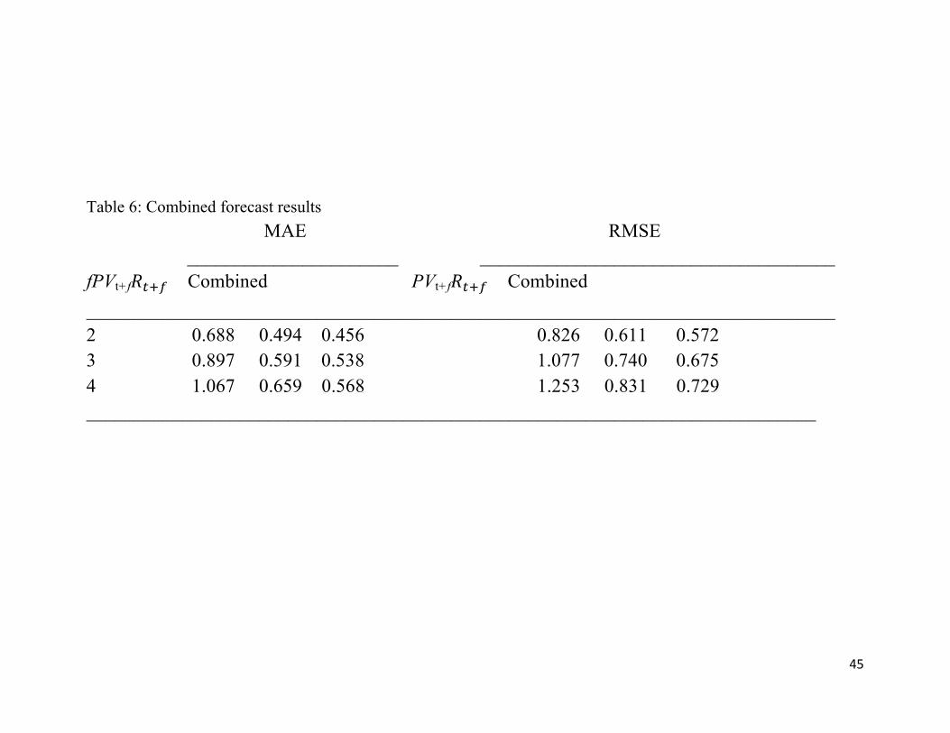
We generate the combined forecasts by using the weights on PVt+f (ranging from 0.191 to
0.307) and the weights on Rt+f (ranging from 0.564 to 0.718) in rows 1-3. Table 6 reports the mean
absolute forecast errors (MAE) and the root mean squared forecast errors (RMSE) of the two-
through four-quarter-ahead VAR, random walk, and combined forecasts.
45
Table 6: Combined forecast results MAE RMSE ______________________ _____________________________________ fPVt+f!"#$ Combined PVt+f!"#$ Combined ______________________________________________________________________________ 2 0.688 0.494 0.456 0.826 0.611 0.572 3 0.897 0.591 0.538 1.077 0.740 0.675 4 1.067 0.659 0.568 1.253 0.831 0.729 ____________________________________________________________________________
4646
Based on the statistics in columns 1, 2, and 3 in Table 6, the combined forecast
has a lower MAE for each forecast horizon. Also, the statistics in columns 4, 5, and 6
indicate that the RMSE is lower for the combined forecasts. This means that the
predictive information in the VAR forecasts help improve forecast accuracy.
CONCLUSION
Accurate forecasts of the interest rate are important to both economic agents in
making sound savings and investment decisions and to policy-makers in making sound
macroeconomic policy decisions. In this paper, we focus on forecasting the 10-year
Treasury bond rate (TBR) using a vector autoregressive (VAR) model for the period 1992-
2016. For comparison, we use the TBR forecasts from the Survey of Professional
Forecasters (SPF) in addition to the random walk forecasts. Our VAR model includes three
variables: the actual TBR, the SPF forecasts of output growth, and the SPF forecasts of
inflation. Our results indicate that the one-through four-quarter-ahead SPF and VAR
forecasts are biased and contain distinct predictive information. However, when
introducing the random walk forecasts along with the SPF and VAR forecasts in the test
equation, the SPF forecasts prove to be inferior to both the VAR and random walk
forecasts. Additional results indicate that the two-through four-quarter-ahead VAR
forecasts contain distinct predictive information from the random walk benchmark. Based
on these results, we combine the VAR and random walk forecasts. Using the MAE and
RMSE statistics, we find that the two-through four-quarter-ahead combined forecasts do
indeed improve accuracy over both the VAR and the random walk forecasts. Hence, we
recommend researchers utilize the SPF forecasts of output growth and inflation in order to
produce accurate forecasts of the TBR.
47
REFERENCES
Baghestani, H. (2009). Forecasting in efficient bond markets: Do experts know
better? International Review of Economics & Finance, 18(4), 624-630.
Baghestani, H. (2010). Forecasting the 10-year US treasury rate. Journal of
Forecasting, 29(8), 673-688.
Baghestani, H., Arzaghi, M., & Kaya, I. (2015). On the accuracy of Blue Chip forecasts of
interest rates and country risk premiums. Applied Economics, 47(2), 113-122.
Brooks, R., & Gray, J. B. (2004).History of the forecasters. The Journal of Portfolio
Management, 31(1), 113-117.
Friedman, B. M. (1980). Survey evidence on the ‘rationality’ of interest rate
expectations. Journal of Monetary Economics, 6(4), 453-465.
Holden, K., & Peel, D. A. (1990).On testing for unbiasedness and efficiency of
forecasts. The Manchester School, 58(2), 120-127.
Mitchell, K., & Pearce, D. K. (2007). Professional forecasts of interest rates and exchange
rates: Evidence from the Wall Street Journal’s panel of economists. Journal of
Macroeconomics, 29(4), 840-854.
Newey, W. K., & West, K. D. (1986).A simple, positive semi-definite, heteroskedasticity
and autocorrelation consistent covariance matrix. Econometrica, 55, 703-708.
Pesando, J. E. (1979). On the random walk characteristics of short-and long-term interest
rates in an efficient market. Journal of Money, Credit and Banking, 11(4), 457-466.
Reichenstein, W. R. (2006). Rationality of naive forecasts of long-term rates. The Journal
of Portfolio Management, 32(2), 116-119.
48
EXAMINING THE IMPACT OF FERTILITY ON FEMALE LABOR FORCE
PARTICIPATION IN NORTH AMERICA AND MEXICO
Sara Almutawa
School of Business Administration American University of Sharjah
Email: [email protected]
ABSTRACT
This paper examines the relationship between female labor force participation rates and
fertility rates in North America (Canada and the United States) and Mexico, a region that
has signed the free trade agreement NAFTA. Utilizing panel data for the period 1991–
2014, we find mixed results across these countries. In particular, our results indicate a
negative (positive) correlation between fertility rates and female labor force participation
rates in Mexico (the US), but no relationship in Canada. As we shall explain, these mixed
results can be attributed to factors such as rising unemployment rates, the rise in women’s
earnings, and the availability of purchased childcare in the market.
Keywords: Female labor participation; Fertility; Panel data analysis; NAFTA countries
49
INTRODUCTION
Female labor participation is an important factor influencing the well-being of the
economy. Aguirre et al. (2012) have shown that raising the female labor force participation
rate to the country-specific male level would increase GDP in the US by 5 percent, Egypt
by 34 percent, and Japan by 9 percent. Thus, it is important to understand the major factors
that influence the female labor force participation rate. The fertility (defined as child-
bearing) rate is an important constraining factor to female employment; the arrival of a
newborn inhibits workforce participation for the woman who has just become a mother in
order to allocate more time towards raising her child (Bernhardt, 1993). Child rearing and
economically productive work are said to be incompatible. Especially in today’s world,
work sites are usually far from home and schedules set by employers lack the flexibility
required to look after children.
In this study, we examine the intriguing question of whether the fertility rate reduces
the female labor force participation rate in North America (Canada and the United States)
and Mexico, a region that has signed the free trade agreement NAFTA. Utilizing panel data
for the period 1991-2014, we find mixed results across these countries. In particular, our
results indicate a negative (positive) correlation between fertility rates and female labor
force participation rates in Mexico (the US), but no relationship in Canada. The mixed
results could be attributed to factors such as, the rising unemployment rates, the rise in
women’s earnings, and the availability of purchased childcare in the market.
This study is organized as follows: section 2 provides the literature review. Section 3
presents the data, empirical results, and interpretations. Section 4 presents the discussion

50
of the results, and section 5 concludes by suggesting further research on certain areas of
this topic.
LITERATURE REVIEW
There is consensus among economists that there generally exists a negative relationship
between fertility and women’s employment. However, the causal nature of the relationship
is less clear and has been the topic of heated debate for many years now. Bumpas and
Westoff (1970, p. 95) were among the earliest to explore the causal nature of the
relationship by asking “Do women limit their fertility in order to pursue their nonfamily-
oriented interests or do women work if their fertility permits them to do so?” As also noted
by Rindfuss and Brewster (2000), the direction of causality could go either way; that is,
fertility could lower female participation, or female participation could lower fertility. In
particular, Weller (1977) cites four possible explanations for the observed negative
relationship between fertility and female labor force participation:
1) Fertility affects labor force participation
2) Labor force participation affects fertility
3) Both women’s fertility and labor force participation affect each other
4) The observed relationship is spurious and is caused by other factors
The literature contains considerable research on the relationship between fertility and
female employment. Some argue that it is fertility that affects labor force participation,
while others argue the opposite. Despite such disagreement, the relationship between the
two remains important for formulating public policies in both developed and developing
countries (Brewster and Rindfuss 2000). Accordingly, in what follows, we divide our

51
literature review by focusing on two strands of research. First, studies that take female
labor force participation as a function of fertility and then studies that take fertility as a
function of female labor force participation.
FEMALE LABOR FORCE PARTICIPATION AS A FUNCTION OF FERTILITY
The presence of children influences a woman’s decision about whether to enter the labor
force or not. Most employed women leave work at some time around birth. It is not
childbearing only but child rearing (the process of taking care of a child from birth to
adulthood) that leads to the negative relationship between fertility and female labor force
participation (Bernhardt 1993). In Germany for instance, women tend to leave the labor
force for an extended period of time following a birth due to the serious shortage of
childcare and school day schedules that vary according to the age of the child (Brewester
and Rindfuss 2000; Schierman 1991). Also, the presence of young children can increase
women’s reservation wage (the wage that makes a woman indifferent between working or
staying at home) which, in turn, lowers the probability of participation (Connelly, 1992).
The hypothesis that fertility hinders women’s participation in the labor market is widely
accepted. Many research studies on the determinants of female labor force participation
rate have thus used fertility rates as one of the independent variables. There are plenty of
studies in the literature that confirm the negative effect that fertility has on female labor
force participation. For instance, Rindfuss et al. (2003) use data on 22 low fertility countries
for 1960-1980 and find that an increase in fertility rates results in a reduction in female
labor force participation rates. One reason that they cite is the incompatibility between
child bearing/rearing and work.

52
Like Rindfus et al. (2000) in the case of the OECD countries, other studies show that
when the fertility rate increases, the female labor force participation decreases. Cruces and
Galiani (2007) focus on Argentina and Mexico to show that an additional child in a family
reduces women’s employment. Knaul and Parker (1997) also focus on Mexico and show
that the presence of one child lowers the probability of women working outside their home
even for part time jobs. However, the probability of working increases when there is
someone to help at home with childcare.
More recent studies suggest a positive relationship between fertility rate and female
labor force participation rate, especially after 1980. According to Engelhardtand Prskawetz
(2004, p.36), “the countries that now have the lowest levels of fertility are those with
relatively low levels of female labor force participation, and the countries with higher
fertility levels tend to have relatively high female force participation rates”. Labor market
institutions, unemployment rate, childcare benefits and government policies are cited as
the reasons for the positive relationship between fertility and female labor force
participation rates.
Ahn and Mira (2002) use panel data on OECD countries from 1970-1995 and show that
the relationship between fertility rate and female labor force participation was negative
during the 1970s and then turned positive after 1980. They cite three possible explanations
for this reversal of relationship, female real wages, childcare, and unemployment rate.
More specifically, as female real wages increase, more and more women choose to work.
As a main determinant of fertility decisions, real wage increases induce both income and
substitution effects on fertility. According to the theory of labor supply, at initially low
wage levels a further increase in wages generates the substitution effect, leading to an

53
increased female labor supply, and fertility would drop for those entering the labor force,
thus resulting in an inverse relationship between fertility and participation. However, at
initially high female wages, a further increase in wages generates an income effect that
leads to higher fertility. Under the fixed hours restriction (no change in hours of work), a
wage increase has the income effect. That is, higher wages will lead to higher fertility
(assuming children are normal goods), resulting in a positive relationship between fertility
and female participation. Thus, the income effect is one factor that could explain the
positive relationship between fertility and female labor force participation.
The second reason cited by Ahn and Mira (2002) is the availability of purchased
childcare in the market, as is the case in some developed countries. The availability of
purchased childcare allows women to allocate more time towards their work, reducing the
incompatibility between work and child rearing and allowing them to have children without
leaving the workforce for a long period of time. On the other hand, the higher the price of
childcare, the lower the fertility rate, which keeps the relationship between fertility and
female employment negative. However, as more women work, there is more political
pressure for generous childcare subsidies, which reduces the price of childcare. Also, due
to the increased demand for jobs that are compatible with childrearing, more jobs are
created with flexible hours of work, and working from home. Thus, childcare affordability
explains the positive relationship between fertility and female participation. In addition,
the income effect of female wage changes on fertility is more important relative to the
substitution effect because the price of childbearing depends less on the mother’s wages
and more on the market price of childcare. Therefore, because of higher wages in the 90’s,
“the effect of higher female wages on fertility becomes less negative or more positive when
54
we consider affordable childcare, facilitating the reversal of the relationship between
fertility and female participation” (Ahn and Mira 2002, p.19).
The third reason cited by Ahn and Mira (2002) for the positive relationship is the rise in
unemployment in the 1980s. Unemployment negatively affects fertility because “more
women will enter the workforce as insurance strategy against the negative shocks to their
husband’s wage or employment” (Ahn and Mira,2002, p.21). Also, fewer women would
leave the labor market to have more children as it could ruin their future job prospects. Ahn
and Mira (2002) argue that countries with lower female participation rates and wages tend
to have higher unemployment rates, which greatly reduces fertility. Again, this could
explain the positive relationship between fertility and female participation.
Other studies give similar explanations for the observed positive relationship. Rocha
and Fuster (2006), for example, investigate the relationship between fertility and female
labor force participation rate in OECD countries for 1986-1995 and find a reversal in the
relationship from negative to positive. The author explains that labor market frictions (i.e.,
the low probability of finding a job) induce females to postpone giving birth or avoid
fertility due to two reasons. First, a decrease in the probability of finding a job increases
the length of a career interruption, which is costly in terms of foregone wages in addition
to a depreciation of human capital. By spacing births, females can avoid a costly career
interruption. Second, since children are costly and, as income is low when females are
young, they may postpone births (Rocha and Fuster, 2005). These two effects intensify as
the unemployment rate increases among females.
Adsera (2004) also studies how different labor market arrangements caused this

55
reversal of trend. She also finds that high unemployment rate and easy accommodation of
the entry-exit of the labor market of the US are two factors responsible for the change in
the relationship. She finds that availability of childcare and part-time work, as well as the
benefits that mothers receive from the job, increases both the likelihood of having a child
and working simultaneously.
Utilizing the Canadian data up to 1995, Engelhardt and Prskawetz (2004) find a
positive relationship between the variables fertility and female labor force participation.
Canada’s population growth rate has not been increasing as much as the US population but
has experienced large migration flows, which could lead to simultaneously lower fertility
rates and lower female labor force participation rates. The pattern of fertility in Canada
differs between native born women and women who migrated to Canada early on. For
instance, a survey conducted by Adsera and Ferer (2014) finds that fertility patterns for
women who migrated to Canada early on tend to be lower than the native born. Immigrants
from Asia and Africa who arrived in Canada early have significantly lower fertility levels
than the Canadian-born. These immigrants tend to have higher levels of schooling and later
fertility than similarly aged native born persons. One reason to explain the lower fertility
is their high educational attainment. At the same time, recent data indicate that 70% of
Canadian labor force consists of immigrants. With growing immigration as the main
contributor to Canada’s labor force in recent years, and the fact that women who migrated
to Canada early on tend to have lower fertility levels than the native born, one may expect
a weaker (or nonexistent) link between fertility rates and female labor force participation
rates.

56
FERTILITY AS A FUNCTION OF FEMALE LABOR FORCE PARTICIPATION
Some studies have shown that the inhibiting effect of fertility on female labor force
participation tends to be short lived; that is, the negative impact of childbearing on labor
force participation ends when the youngest child reaches school age(Brewster and Rinfuss
2000; Waite and Stolzenberg 1976; Hout 1978; Smith-Lovin and Tickameyer 1978). In
particular, the effect of labor force participation on fertility tends to be weaker in the short-
run but stronger in the long-run. According to Cramer (1980) current employment lowers
both actual and expected fertility, and since this builds up over time, employment may in
the long run have a great effect on fertility(Bernhardt 1993). The studies by Cramer (1980)
and other studies suggest that the dominant effect in the short-run is from fertility to female
employment, and from employment to fertility in the long-run. However, these studies have
been highly criticized for having statistical shortcomings. Despite this, the negative impact
of female labor force participation on fertility has a theoretically strong foundation
(Brewster and Rindfuss, 2000).
More specifically, economic theory suggests that an increase in the opportunity costs of
having children should be associated with lower fertility rates (Lehrer and Nerlove 1986).
Labor force participation is known to increase the opportunity cost of childbearing in terms
of foregone wage earnings and could reduce the time left for leisure (Brewster and
Rindfuss, 2000). Accordingly, it is not surprising that women in the labor force tend to
have lower fertility levels on average than women who are out of the labor force (United
Nations, 1976). Economic theory also suggests that mothers who have greater stocks of
human capital have higher opportunity costs associated with child bearing and rearing
(Lehrer and Nerlove 1986).

57
One of the ways in which fertility rates decline due to an increase in female labor force
participation is through women delaying the transition to parenthood. For example, one
survey found that in the US, married women with paid jobs are more likely than married
women who do not work to postpone the birth of their first child (Brewster and Rindfuss
2000; Blau and Robins, 1988). These decisions reflect the higher opportunity costs for
childbearing among women with high human capital and earnings.
However, studies investigating the impact of employment on fertility have been
inconclusive due to a number of reasons. Some studies indicate that the observed
relationship between higher employment and lower fertility is just a matter of the choice
of lifestyle. Women who want to work longer tend to also have lower fertility ambitions
(Bernhardt 1993). For instance, Hoem and Hoem (1989) tested the hypothesis that the
opportunity cost of a second or third birth is higher for Swedish women with better
education or with a secure position in the labor force. Their results indicate that the effect
of present employment and those who have spent the most time in the labor force since the
birth of the first child on the propensity for a third birth among mothers with two children
is not different from mothers who are primarily housewives. Also, there was no difference
on the effect of employment on fertility among woman who worked full time or part-time.
Surprisingly, the excess risk of third births among housewives has reduced over time, while
that of working women has been more stable. A woman’s personal values rather than
employment seem to be a stronger determinant of her choice to have more children.
DATA, EMPIRICAL RESULTS, AND INTERPRETATIONS
In line with most of the literature, we focus on investigating the female labor force
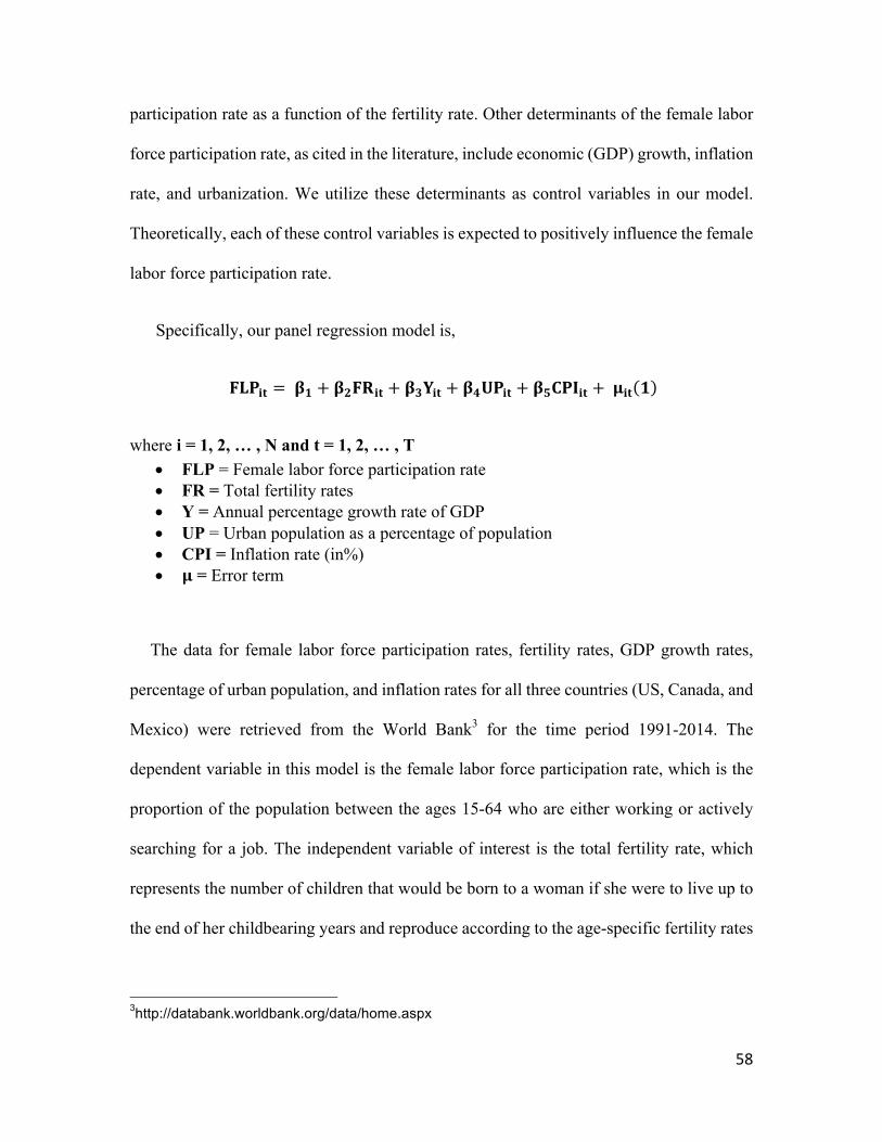
58
participation rate as a function of the fertility rate. Other determinants of the female labor
force participation rate, as cited in the literature, include economic (GDP) growth, inflation
rate, and urbanization. We utilize these determinants as control variables in our model.
Theoretically, each of these control variables is expected to positively influence the female
labor force participation rate.
Specifically, our panel regression model is,
#$%&' = )* + ),#-&' + )./&' + )01%&' + )23%4&' +5&' *
where i = 1, 2, … , N and t = 1, 2, … , T • FLP = Female labor force participation rate • FR = Total fertility rates • Y = Annual percentage growth rate of GDP • UP = Urban population as a percentage of population • CPI = Inflation rate (in%) • 5 = Error term
The data for female labor force participation rates, fertility rates, GDP growth rates,
percentage of urban population, and inflation rates for all three countries (US, Canada, and
Mexico) were retrieved from the World Bank3 for the time period 1991-2014. The
dependent variable in this model is the female labor force participation rate, which is the
proportion of the population between the ages 15-64 who are either working or actively
searching for a job. The independent variable of interest is the total fertility rate, which
represents the number of children that would be born to a woman if she were to live up to
the end of her childbearing years and reproduce according to the age-specific fertility rates
3http://databank.worldbank.org/data/home.aspx

59
for the specified year (World Bank, 2014). Table1 reports the descriptive statistics for both
the female labor force participation rate and the fertility rate.
As can be seen from Table 1 the mean value of female labor force participation rate in
Mexico (42.64) is much lower than those for Canada and the US. However, the mean value
of the fertility rate in Mexico happens to be well above those for Canada and the US.
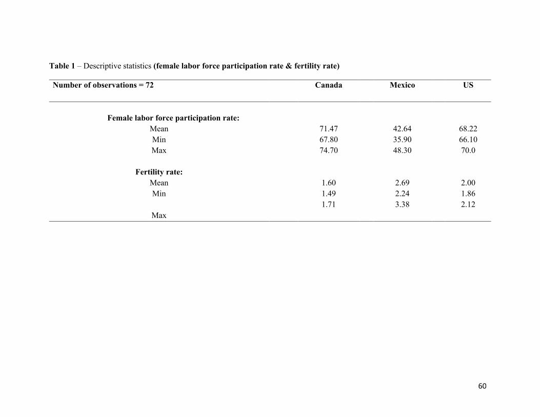
6046
Table 1 – Descriptive statistics (female labor force participation rate & fertility rate)
Number of observations = 72 Canada Mexico US
Female labor force participation rate:
Mean 71.47 42.64 68.22 Min 67.80 35.90 66.10 Max 74.70 48.30 70.0
Fertility rate:
Mean 1.60 2.69 2.00 Min 1.49 2.24 1.86
Max 1.71 3.38 2.12

6146
As for the control variables in Equation (1), we have: the annual percentage growth rate
of GDP, the percentage of people living in urban areas, and the inflation rate. They are all
included to account for the positive relationship between them and the female labor force
participation rate. The method of estimation is ordinary least squares (OLS) panel
regression with the standard errors corrected for heteroscedasticity and autocorrelation
using the Newey-West procedure. The total number of observations is 72.
Column 1 of Table 2 reports the regression estimates of Equation (1). Of the control
variables, urbanization has the correct sign and is significant in determining the female
labor force participation rate. However, both GDP growth and inflation rate are
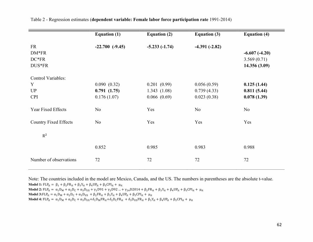
6246
Note: The countries included in the model are Mexico, Canada, and the US. The numbers in parentheses are the absolute t-value. Model 1: FLP$% = β) + β+FR$% + β-Y$% + β/UP$% + β1CPI$% + µ$% Model 2:FLP$% = α)D7 + α+D8 + α-D9: + γ)D91 + γ+D92…+ γ+/D2014 + β+FR$% + β-Y$% + β/UP$% + β1CPI$% + µ$% Model 3:FLP$% = α)D7 + α+D8 + α-D9: + β+FR$% + β-Y$% + β/UP$% + β1CPI$% + µ$% Model 4:FLP$% = α)D7 + α+D8 + α-D9:+B)D7FR$%+B+D8FR$% + B-D9:FR$% + β-Y$% + β/UP$% + β1CPI$% + µ$%
Table 2 - Regression estimates (dependent variable: Female labor force participation rate 1991-2014)
Equation (1) Equation (2) Equation (3) Equation (4) FR -22.700 (-9.45) -5.233 (-1.74) -4.391 (-2.82) DM*FR -6.607 (-4.20) DC*FR 3.569 (0.71) DUS*FR 14.356 (3.09) Control Variables: Y 0.090 (0.32) 0.201 (0.99) 0.056 (0.59) 0.125 (1.44) UP 0.791 (1.75) 1.343 (1.08) 0.739 (4.33) 0.811 (5.44) CPI 0.176 (1.07) 0.066 (0.69) 0.023 (0.38) 0.078 (1.39) Year Fixed Effects No Yes No No Country Fixed Effects No Yes Yes Yes 0.852 0.985 0.983 0.988 Number of observations
72
72
72
72
R+
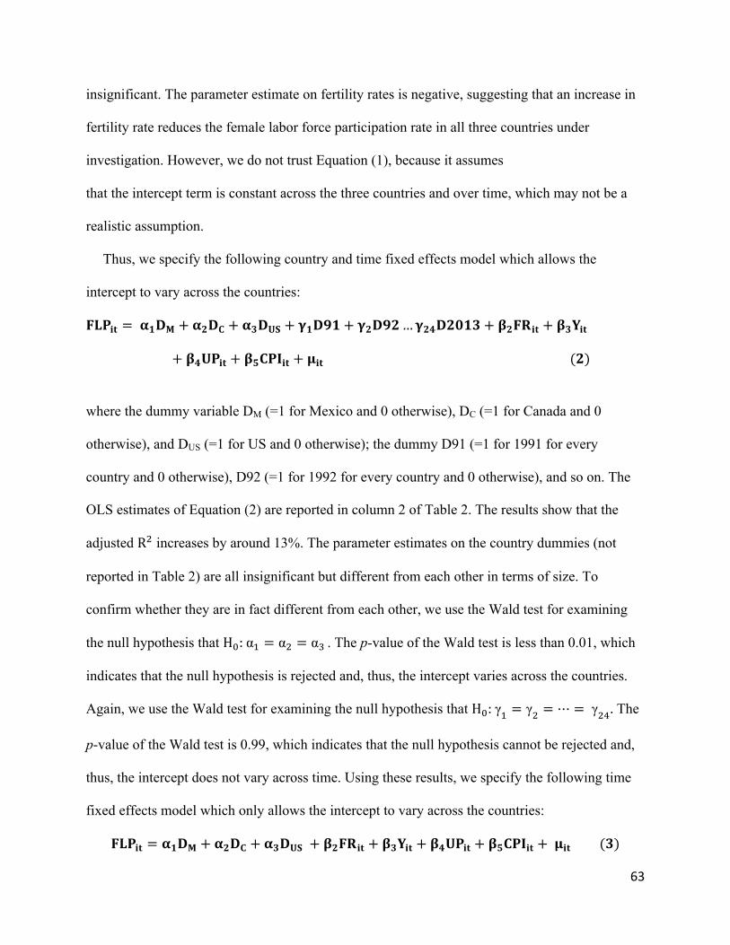
63
insignificant. The parameter estimate on fertility rates is negative, suggesting that an increase in
fertility rate reduces the female labor force participation rate in all three countries under
investigation. However, we do not trust Equation (1), because it assumes
that the intercept term is constant across the three countries and over time, which may not be a
realistic assumption.
Thus, we specify the following country and time fixed effects model which allows the
intercept to vary across the countries:
!"#$% = ()*+ + (-*. + (/*01 + 2)*3) + 2-*3-…2-5*-6)/ + 7-!8$% + 7/9$%
+ 750#$% + 7:.#;$% + <$%(-)
where the dummy variable DM (=1 for Mexico and 0 otherwise), DC (=1 for Canada and 0
otherwise), and DUS (=1 for US and 0 otherwise); the dummy D91 (=1 for 1991 for every
country and 0 otherwise), D92 (=1 for 1992 for every country and 0 otherwise), and so on. The
OLS estimates of Equation (2) are reported in column 2 of Table 2. The results show that the
adjusted R@ increases by around 13%. The parameter estimates on the country dummies (not
reported in Table 2) are all insignificant but different from each other in terms of size. To
confirm whether they are in fact different from each other, we use the Wald test for examining
the null hypothesis that HB:αD = α@ = αE. The p-value of the Wald test is less than 0.01, which
indicates that the null hypothesis is rejected and, thus, the intercept varies across the countries.
Again, we use the Wald test for examining the null hypothesis that HB:γD = γ@ = ⋯ = γ@G. The
p-value of the Wald test is 0.99, which indicates that the null hypothesis cannot be rejected and,
thus, the intercept does not vary across time. Using these results, we specify the following time
fixed effects model which only allows the intercept to vary across the countries:
!"#$% = ()*+ + (-*. + (/*01 + 7-!8$% + 7/9$% + 750#$% + 7:.#;$% +<$%(/)
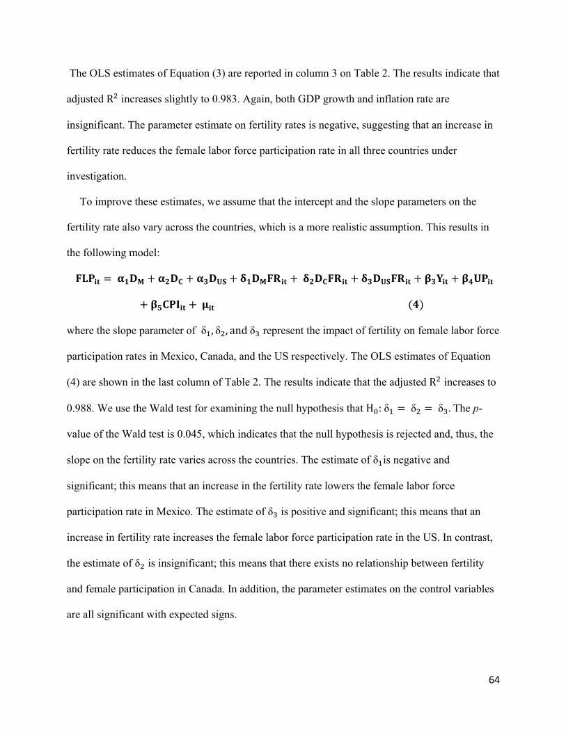
64
The OLS estimates of Equation (3) are reported in column 3 on Table 2. The results indicate that
adjusted R@ increases slightly to 0.983. Again, both GDP growth and inflation rate are
insignificant. The parameter estimate on fertility rates is negative, suggesting that an increase in
fertility rate reduces the female labor force participation rate in all three countries under
investigation.
To improve these estimates, we assume that the intercept and the slope parameters on the
fertility rate also vary across the countries, which is a more realistic assumption. This results in
the following model:
!"#$% = ()*+ + (-*. + (/*01 + I)*+!8$% +I-*.!8$% + I/*01!8$% + 7/9$% + 750#$%
+ 7:.#;$% +<$%(5)
where the slope parameter of δD, δ@, andδE represent the impact of fertility on female labor force
participation rates in Mexico, Canada, and the US respectively. The OLS estimates of Equation
(4) are shown in the last column of Table 2. The results indicate that the adjusted R@ increases to
0.988. We use the Wald test for examining the null hypothesis that HB:δD = δ@ = δE.The p-
value of the Wald test is 0.045, which indicates that the null hypothesis is rejected and, thus, the
slope on the fertility rate varies across the countries. The estimate of δDis negative and
significant; this means that an increase in the fertility rate lowers the female labor force
participation rate in Mexico. The estimate of δE is positive and significant; this means that an
increase in fertility rate increases the female labor force participation rate in the US. In contrast,
the estimate of δ@ is insignificant; this means that there exists no relationship between fertility
and female participation in Canada. In addition, the parameter estimates on the control variables
are all significant with expected signs.
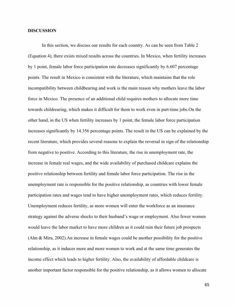
65
DISCUSSION
In this section, we discuss our results for each country. As can be seen from Table 2
(Equation 4), there exists mixed results across the countries. In Mexico, when fertility increases
by 1 point, female labor force participation rate decreases significantly by 6.607 percentage
points. The result in Mexico is consistent with the literature, which maintains that the role
incompatibility between childbearing and work is the main reason why mothers leave the labor
force in Mexico. The presence of an additional child requires mothers to allocate more time
towards childrearing, which makes it difficult for them to work even in part-time jobs.On the
other hand, in the US when fertility increases by 1 point, the female labor force participation
increases significantly by 14.356 percentage points. The result in the US can be explained by the
recent literature, which provides several reasons to explain the reversal in sign of the relationship
from negative to positive. According to this literature, the rise in unemployment rate, the
increase in female real wages, and the wide availability of purchased childcare explains the
positive relationship between fertility and female labor force participation. The rise in the
unemployment rate is responsible for the positive relationship, as countries with lower female
participation rates and wages tend to have higher unemployment rates, which reduces fertility.
Unemployment reduces fertility, as more women will enter the workforce as an insurance
strategy against the adverse shocks to their husband’s wage or employment. Also fewer women
would leave the labor market to have more children as it could ruin their future job prospects
(Ahn & Mira, 2002).An increase in female wages could be another possibility for the positive
relationship, as it induces more and more women to work and at the same time generates the
income effect which leads to higher fertility. Also, the availability of affordable childcare is
another important factor responsible for the positive relationship, as it allows women to allocate

66
more time toward their work as well as it allows them to have children without leaving the
workforce for a long period of time.
In contrast, in Canada there exists no significant relationship between fertility and female
labor force participation. This result is unexpected and could be due to an external factor, such as
migration. More specifically, migration could simultaneously lead to both lower fertility and
lower female labor force participation since most of Canada’s labor force is made up of
immigrants and research indicates that Canadian immigrants tend to have lower fertility levels
than the Canadian-born. Our results indicate a positive relationship but not significant.
CONCLUSION
In conclusion, the relationship between fertility and female participation is important for
policy decisions in both developed and developing countries. Although the direction of causality
between the two variables has been less clear. However, many studies use female labor force
participation as a function of fertility rather than vice versa. In line with these studies, we take
female labor force participation as a function of fertility. We find mixed results; female labor
force participation rate is negatively correlated with fertility rate in Mexico due to perhaps the
high level of role incompatibility between childbearing and work. While in the US the
correlation turned positive due to the recent explanations in the literature, such as the increase in
female real wages, the rise in unemployment rates, and the availability of purchased childcare,
which reduces the role incompatibility between child rearing and work. Furthermore, there exists
a positive but insignificant correlation between the two variables in Canada. Future studies
should investigate the reasons for the absence of correlation between female labor force
participation and fertility in Canada. We also recommend further research on the relationship

67
between fertility and female labor force participation by including factors such as female real
wages, unemployment rates, availability of market childcare, and maternity benefits in the
model, in order to examine how each of these factors could possibly influence the relationship
between the two variables.
68
REFERENCES
Adsera, A. (2004) Changing fertility rates in developed countries: The impact of labor
market institutions. Journal of Population Economics 17, 17-43.
Adsera, A. and A. Ferrer (2014). Fertility adaptation of child migrants to Canada.
Population Studies68, 65-79.
Aguirre, D., L. Hoteit, C. Rupp, and K. Sabbagh (2012). Empowering the Third Billion.
Women and the World of Work in 2012. Retrieved from Booz and Company:
http://www.strategyand.pwc.com/media/file/Strategyand_Empowering-the-Third-
Billion_Full-Report.pdf
Ahn, N. and P. Mira (2002). A note on the changing relationship between fertility and
female employment rates in developed countries. Journal of Population Economics
15, 667-682.
Bernhardt, E. M. (1993). Fertility and employment. European Sociological Review 9, 25-
42.
Brewster, K. L. and R.R. Rindfuss (2000). Fertility and women's employment in
industrialized nations. Annual Review of Sociology26, 271-296.
Connelly, R. (1992). The effect of child care costs on married women’s labor force
participation. The Review of Economics and Statistics74, no. 1, 83-9.
Cramer, J. C. (1980). Fertility and female employment: Problems of causal
direction.American Sociological Review 45, 167-190.
69
Cruces, G. and S. Galiani (2007). Fertility and female labor supply in Latin America: New
causal evidence. Labour Economics 14, 565-573.
Engelhardt, H. and A. Prskawetz (2004). On the changing correlation between fertility and
female employment over space and time. European Journal of Population 20, 35-
62.
Hoem, B. and J.M. Hoem (1989) The impact of women's employment on second and third
births in modern Sweden. Population Studies43, 47-67.
Knaul, F. and S.W. Parker (1997) Employment and child care strategies among Mexican
women with young children.CIDE Working Paper DTE 75,
Mexico.http://aleph.academica.mx/jspui/handle/56789/4036
Lehrer, E., and M. Nerlove (1986). Female labor force behavior and fertility in the United
States. Annual Review of Sociology12, 181-204.
Rocha, J. M. and L. Fuster (2006). Why are fertility rates and female employment ratios
positively correlated across O.E.C.D. countries? International Economic Review47,
1187-1222.
Rindfuss,R., K. Guzzo, and S.Morgan (2003). The changing institutional context of low
fertility. Population Research and Policy Review22, 411-438.
United Nations (1976). Fertility and Family Planning in Europe around 1970: A
Comparative Study of Twelve National Surveys. New York: United Nations.
Weller, R. H. (1977). Wife’s employment and cumulative family size in the United States,
1970 and 1960. Demography14, 43-65.